Hyperfine meson splittings: chiral symmetry versus transverse gluon exchange

Abstract

Meson spin splittings are examined within an effective Coulomb gauge QCD Hamiltonian incorporating chiral symmetry and a transverse hyperfine interaction necessary for heavy quarks. For light and heavy quarkonium systems the pseudoscalar-vector meson spectrum is generated by approximate BCS-RPA diagonalizations. This relativistic formulation includes both $S$ and $D$ waves for the vector mesons which generates a set of coupled integral equations. A smooth transition from the heavy to the light quark regime is found with chiral symmetry dominating the $\pi$-$\rho$ mass difference. A reasonable description of the observed meson spin splittings and chiral quantities, such as the quark condensate and the $\pi$ mass, is obtained. Similar comparisons with TDA diagonalizations, which violate chiral symmetry, are deficient for light pseudoscalar mesons indicating the need to simultaneously include both chiral symmetry and a hyperfine interaction. The $\eta_{b}$ mass is predicted to be around 9400 MeV consistent with other theoretical expectations and above the unconfirmed 9300 MeV candidate. Finally, for comparison with lattice results, the $J$ reliability parameter is also evaluated.

I Introduction

The hyperfine interaction has a long and distinguished history beginning with the hydrogen atom where it correctly describes the transition responsible for the famous “21-centimeter line” in microwave astronomy. Taking the non-relativistic reduction of the one-photon-exchange interaction, the hyperfine potential has the form

$$V_{hyp}={\rm const}\ \frac{\bm{\sigma}_{1}}{M_{1}}\cdot\frac{\bm{\sigma}_{2}}{M_{2}}\delta(\bm{r})$$ (1)

for particles of mass $M_{i}$ and spin $\bm{\sigma}_{i}$. This potential gives an accurate description of the triplet-singlet splitting in positronium. When implemented in the simple additive quark model having meson mass $M$ and constituent quark masses ${\cal M}_{q=u,d,s}$ ,

$$M={\cal M}_{q}+{\cal M}_{\bar{q}}+A\frac{\bm{\sigma}_{q}}{{\cal M}_{q}}\cdot\frac{\bm{\sigma}_{\bar{q}}}{{\cal M}_{\bar{q}}}$$ (2)

it produces a remarkably good description of the light meson spectrum using $A\approx 160\ {\cal M}^{2}_{u}$ MeV. However, to reproduce the splitting in charmonium, using ${\cal M}_{q=c}$ $\approx 1500$ MeV, requires a hyperfine strength of at least $4A$, while a similar model for baryons uses a much weaker value, approximately $A/3$ grif . Hence attempts to comprehensively describe spin splittings in hadrons with a simple hyperfine interaction leads to over an order of magnitude variation in the potential strength. Although this may merely reflect the simplistic nature of the additive quark model, more extensive models also have difficulty in obtaining a consistent description for both mesons and baryons with the same hyperfine interaction. Possibly related, other problems arise when considering the hyperfine interaction in quark model applications. For example, the non-relativistic reduction of the one gluon exchange interaction between quark pairs gives rise to hyperfine, spin-orbit and tensor interactions at order $1/{\cal M}_{q}^{2}$. Unfortunately this structure does not describe heavy meson spin splittings well and must be supplemented with a spin-orbit term which is argued gi to emerge from the reduction of a scalar confinement potential. Although this prescription is reasonably successful for heavy mesons, it generates too large spin-orbit splittings in baryons ci and the sign of the scalar confinement potential must be inverted sspot .

Further clouding this matter is the role of chiral symmetry. Because the pion is regarded as the Goldstone boson of broken chiral symmetry, the $\pi$-$\rho$ mass difference should be dominated by the same nonperturbative dynamics producing spontaneous chiral symmetry breaking Scadron ; brs96 ; mrt98 ; csref . This observation is in conflict with the hyperfine splitting in typical constituent (non-chiral) quark models which apply Eq. (1) to light hadrons. Indeed in such models the hyperfine potential plays a dual role of generating spin splittings and producing a very light, “chiral” pseudoscalar meson. Because of the quite large, over 600 MeV, $\pi$-$\rho$ and 400 MeV $K$-$K^{*}$ mass differences, an appreciable hyperfine splitting is required. This in turn makes it necessary to use a more complex interaction, rather than a simple potential, to simultaneously describe hadrons not governed by chiral symmetry, such as excited state light mesons, heavy mesons and baryons which all have smaller spin splittings, roughly from 50 to 300 MeV. As discussed in Ref. ess , the nonperturbative aspects of spin splittings in light quark hadrons, especially those involving pseudoscalar mesons, clearly requires a more sophisticated model treatment.

The purpose of this paper is to address the above issues and to provide a deeper understanding of meson spin splittings by examining the hyperfine interaction in a theoretical framework which incorporates chiral symmetry. A related goal is to also provide an improved hadron approach embodying many of the features of QCD with a minimal number of parameters (i.e. current quark masses and one or two dynamical constants). This formulation is based on the Coulomb gauge Hamiltonian of QCD and approximate diagonalizations using the Bardeen-Cooper-Schrieffer (BCS), Tamm-Dancoff (TDA) and random phase approximation (RPA) many-body techniques. These methods have been previously applied to chiral symmetry breaking orsay , glueballs gbs ; lcbrs ; gss , hybrids sshyb ; lcplb and mesons LC1 ; LC2 ; ls2 . The renormalization group methodology has also been appliedssrenorm ; rob to improve this formalism. Finally, this work incorporates an effective QCD longitudinal confining potential sspot along with a generalized version of the transverse hyperfine interaction employed in an earlier hyperfine study sshyp .

An important aspect of the following discussion is that the random phase approximation is capable of describing chiral symmetry breaking. Indeed, the RPA pion mass, $M_{\pi}$, satisfies the Gell-Mann-Oakes-Renner relation dictated by chiral symmetry

$$M_{\pi}=\left[-\frac{2m_{q}\langle\bar{q}q\rangle}{f_{\pi}^{2}}\right]^{1/2}\ ,$$ (3)

where $m_{q}$ is the current quark mass, $f_{\pi}$ is the pion decay constant and $\langle\bar{q}q\rangle\equiv\langle 0|\bar{\Psi}\Psi|0\rangle$ is the quark condensate. In contrast, the TDA does not respect chiral symmetry (the RPA, but not TDA, meson field operator commutes with the chiral charge LC1 ; LC2 ). Comparing RPA and TDA masses therefore permits a quantitative assessment of the relative importance of both chiral symmetry and the hyperfine interaction for the $\pi$-$\rho$ mass splitting. A key result of this work is that chiral symmetry dominates this splitting and accounts for about 400 MeV of the mass difference. Another is that with the same interaction, the mass differences between the radially excited $\pi$ and $\rho$ states are also reproduced, as well as the pseudoscalar and vector states in charmonium and bottomonium, thereby demonstrating the universality of this approach. Lastly, the inclusion of the hyperfine interaction improves the model description of the quark condensate.

In the next section the model Hamiltonian is specified and the BCS and RPA equations are formulated. Section III presents numerical results and details sensitivity to different hyperfine interactions. Finally, conclusions are presented in section IV.

II Effective Hamiltonian and equations of motion

II.1 Model Hamiltonian

As discussed above, the model Hamiltonian is taken to be that of Coulomb gauge QCD. The Coulomb potential is evaluated self-consistently in the mean-field gaussian variational ansatz sspot . The general form of this effective Hamiltonian in the combined quark and glue sectors is

$$H_{eff} = H_{q}+H_{g}+H_{qg}+V_{C}$$ (4)

$$H_{q} = \int d{\bf x}\Psi^{\dagger}({\bf x})(-i\bm{\alpha}\cdot\bm{\nabla}+m_{q}\beta)\Psi({\bf x})$$ (5)

$$H_{g} = Tr\int d{\bf x}\left[{\bf\Pi}^{a}({\bf x})\cdot{\bf\Pi}^{a}({\bf x})+{\bf B}^{a}({\bf x})\cdot{\bf B}^{a}({\bf x})\right]$$ (6)

$$H_{qg} = g\int d{\bf x}{\bf J}^{a}({\bf x})\cdot{\bf A}^{a}({\bf x})$$ (7)

$$V_{C} = -\frac{1}{2}\int d{\bf x}d{\bf y}\rho^{a}({\bf x})\hat{V}(\arrowvert{\bf x}-{\bf y}\arrowvert)\rho^{a}({\bf y})\ .$$ (8)

Here $g$ is the QCD coupling, $\Psi$ is the quark field, ${\bf A}^{a}$ are the gluon fields satisfying the transverse gauge condition, $\nabla$ $\cdot$ ${\bf A}^{a}=0$, $a=1,2,...8$, ${\bf\Pi}^{a}$ are the conjugate fields and ${\bf B}^{a}$ are the nonabelian magnetic fields

$${\bf B}^{a}=\nabla\times{\bf A}^{a}+\frac{1}{2}gf^{abc}{\bf A}^{b}\times{\bf A}^{c}\ .$$ (9)

The color densities, $\rho^{a}({\bf x})$, and quark color currents, ${\bf J}^{a}$, are related to the fields by

$$\rho^{a}({\bf x}) = \Psi^{\dagger}({\bf x})T^{a}\Psi({\bf x})+f^{abc}{\bf A}^{b}({\bf x})\cdot{\bf\Pi}^{c}({\bf x})$$ (10)

$${\bf J}^{a} = \Psi^{\dagger}({\bf x})\mbox{\boldmath$\alpha$\unboldmath}T^{a}\Psi({\bf x})\ ,$$ (11)

where $T^{a}=\frac{\lambda^{a}}{2}$ and $f^{abc}$ are the $SU_{3}$ color matrices and structure constants, respectively.

Since this work focuses on the quark sector $H_{g}$ is omitted and the quark-glue interaction, $H_{qg}$, is replaced by an effective transverse hyperfine potential, $V_{T}$, discussed below. The choice for the longitudinal Coulomb potential, $V_{C}$, then completes specification of the model.

To lowest order in $g$, the Coulomb gauge potential $\hat{V}$ is simply proportional to $1/r$. As is well known, in a few body truncation this is insufficient for confinement and fails to reproduce the phenomenological meson spectrum. Using the Cornell potential for $\hat{V}$ resolves these issues but produces an ultraviolet behavior necessitating the introduction of a model momentum cutoff. Instead, an improved dynamical treatment sspot is adopted in which both the gluonic quasiparticle basis and the confining interaction were determined self-consistently and, through renormalization, accurately reproduced the lattice Wilson loop potential. The resulting interaction has a renormalization improved short ranged behavior and long-ranged confinement. It is similar to the Cornell potential and has a numerical representation in momentum space that is accurately fit by the analytic form

$$V(p)=\left\{\begin{array}[]{ll}C(p)\equiv-\frac{8.07}{p^{2}}\,\frac{{\rm log}^{-0.62}\left(\frac{p^{2}}{m_{g}^{2}}+0.82\right)}{{\rm log}^{0.8}\left(\frac{p^{2}}{m_{g}^{2}}+1.41\right)}&{\rm for}\ p>m_{g}\\ L(p)\equiv-\frac{12.25\,m_{g}^{1.93}}{p^{3.93}}&{\rm for}\ p<m_{g}\ .\end{array}\right.$$ (12)

The low momentum component is numerically close to a pure linear potential, $L\simeq-8\pi\sigma/p^{4}$. The other term represents a renormalized high energy Coulomb tail. The only free parameter is $m_{g}\approx 600$ MeV which sets the scale of the theory and is equivalent to a string tension.

Both the exact and model QCD Coulomb gauge Hamiltonians do not explicitly contain a hyperfine-type interaction, however, perturbatively integrating out gluonic degrees of freedom generates a quark hyperfine interaction with the form $\bm{\alpha}_{1}\cdot\bm{\alpha}_{2}$. One can also formally generate this Lorentz structure using Maxwell’s equations to substitute for the gluon fields in Eq. (7). More generally, in the Hamiltonian formalism an effective hyperfine interaction arises from nonperturbative mixing of gluonic excitations (such as hybrids) with the quark Fock space components of a hadron’s wavefunction. However, the $\bm{\alpha}_{1}\cdot\bm{\alpha}_{2}$ Lorentz structure is expected to persist aspk and Ref. aspk obtains a $\bm{\alpha}_{1}\cdot\bm{\alpha}_{2}$ hyperfine potential with specific spatial form using the linked cluster expansion method to eliminate hybrid intermediate states.

Because contributions from gluonic excitations and hybrid states are difficult to calculate, this work studies several different parameterizations of the following generic transverse hyperfine interaction

$$V_{T}=\frac{1}{2}\int d{\bf x}d{\bf y}J^{a}_{i}({\bf x})\hat{U}_{ij}({\bf x},{\bf y})J^{a}_{j}({\bf y})\ ,$$ (13)

where the kernel $\hat{U}_{ij}$ has the structure

$$\hat{U}_{ij}({\bf x},{\bf y})=\left(\delta_{ij}-\frac{\nabla_{i}\nabla_{j}}{\nabla^{2}}\right)_{\bf x}\hat{U}(|{\bf x}-{\bf y}|)\ ,$$ (14)

reflecting the transverse gauge condition. In specifying the potential $\hat{U}$ it is useful to realize that perturbatively $\hat{U}\rightarrow\alpha_{s}/|{\bf x}-{\bf y}|$ where $\alpha_{s}=g^{2}/4\pi$. Also, the form of the one gluon exchange potential and the nonperturbative mixing with hybrids makes it clear that the hyperfine kernel should not include a confining term. This is important for infrared divergent gap equations Bicudo3 . Consistent with these points, the following four kernels are utilized and numerically compared to document hyperfine model sensitivity.

The non-relativistic quark model advocates a regulated contact interaction gi . Thus model 1 is a simple square well interaction defined by

$$U_{1}(p)=\left\{\begin{array}[]{ll}0&{\rm for}\ p>\Lambda\\ -U_{h}&{\rm for}\ p<\Lambda\end{array}\right.$$ (15)

with strength, $U_{h}$, and range, $\Lambda$.

Model 2 is a variation of a pure Coulomb potential (reflecting a transverse zero mass gluon exchange) and is

$$U_{2}(p)=\left\{\begin{array}[]{ll}C(p)&{\rm for}\ p>m_{g}\\ -\frac{C_{h}}{p^{2}}&{\rm for}\ p<m_{g}\ .\end{array}\right.$$ (16)

Similarly, model 3 incorporates a modified Coulomb potential corresponding to an ultraviolet Coulomb tail matched to a constant in the infrared. This potential is

$$U_{3}(p)=\left\{\begin{array}[]{ll}C(p)&{\rm for}\ p>m_{g}\\ -C_{h}&{\rm for}\ p<m_{g}\ .\end{array}\right.$$ (17)

Finally, model 4 is a Yukawa-type potential corresponding to the exchange of a constituent gluon with a dynamical mass. This is given by

$$U_{4}(p)=\left\{\begin{array}[]{ll}C(p)&{\rm for}\ p>m_{g}\\ -\frac{C_{h}}{p^{2}+m_{g}^{2}}&{\rm for}\ p<m_{g}\ .\end{array}\right.$$ (18)

For the latter three models, the Coulomb potential $C(p)$ is the same as in Eq. (12) and the constant, $C_{h}$, is determined by matching the high and low momentum regions at the transition scale $m_{g}$. In this analysis several different matching points (e.g. $p=m_{g},2m_{g},3m_{g}$) for a given transition scale $m_{g}$ were numerically examined but no qualitative differences were found.

In the following, angular integrals are denoted by

$$V_{n}(k,q)\equiv\int_{-1}^{1}dxV(\arrowvert{\bf k}-{\bf q}\arrowvert)x^{n}$$ (19)

where $x=\hat{\bf k}\cdot\,\hat{{\bf q}}$. The auxiliary functions

$$W({|\bf k}-{\bf q}|)\equiv U(|{\bf k}-{\bf q}|)\frac{x(k^{2}+q^{2})-qk(1+x^{2})}{\arrowvert{\bf k}-{\bf q}\arrowvert^{2}}$$ (20)

and

$$Z(|{\bf k}-{\bf q}|)\equiv U(|{\bf k}-{\bf q}|)\frac{1-x^{2}}{\arrowvert{\bf k}-{\bf q}\arrowvert^{2}}$$ (21)

are also introduced which arise from the operator structure of Eq. (14).

II.2 Gap equation

Calculations are most conveniently made in momentum space with constituent quark operators. These are

obtained by a Bogoliubov transformation (BCS rotation) from the current quark basis to a quasiparticle quark basis represented by particle, $B$, and antiparticle, $D$, operators

$$\Psi({\bf x})=\int\frac{d{\bf k}}{(2\pi)^{3}}e^{i{\bf k}\,\!\cdot\!\,{\bf x}}\sum_{\lambda i}({\cal U}_{{\bf k}\lambda}B_{{\bf k}\lambda i}+{\cal V}_{-{\bf k}\lambda}D^{\dagger}_{-{\bf k}\lambda i})\hat{\epsilon}_{i}$$ (22)

where $\hat{\epsilon}_{i}$ is a color vector with $i=$ 1, 2, 3 and $\lambda$ denotes helicity. The Dirac spinors are functions of the Bogoliubov gap angle $\phi_{k}$ and can be express in terms of the Pauli spinors $\chi_{\lambda}$

$${\cal U}_{{\bf k}\lambda} = \frac{1}{\sqrt{2}}\left[\begin{array}[]{l}\sqrt{1+\sin\phi_{k}}\,\,\chi_{\lambda}\\ \sqrt{1-\sin\phi_{k}}\,\bm{\sigma}\cdot\hat{{\bf k}}\,\,\chi_{\lambda}\end{array}\right]$$ (25)

$${\cal V}_{{\bf-k}\lambda} = \frac{1}{\sqrt{2}}\left[\begin{array}[]{l}-\sqrt{1-\sin\phi_{k}}\,\,\bm{\sigma}\cdot\hat{\bf k}\,\,i\sigma_{2}\chi_{\lambda}\\ \sqrt{1+\sin\phi_{k}}\,\,i\sigma_{2}\chi_{\lambda}\end{array}\right]\ .$$ (28)

Note the additional factor $i\sigma_{2}$ in the spinor $\cal V_{{\bf-k}\lambda}$ which differs from the convention used in Refs. LC1 ; LC2 . The Bogoliubov angle can be related to a running quark mass, $M_{q}(k)$, and energy, $E(k)=\sqrt{M^{2}_{q}(k)+k^{2}}$, by

$$s_{k} \equiv \sin\phi_{k}=\frac{M_{q}(k)}{E(k)}$$ (29)

$$c_{k} \equiv \cos\phi_{k}=\frac{k}{E(k)}\ .$$ (30)

At high $k$, $M_{q}(k)\rightarrow m_{q}$, while for low $k$ a constituent quark mass can be extracted, $\mathcal{M}_{q}=M_{q}(0)$.

Minimizing the vacuum energy with respect to the gap angle yields the mass gap equation

$$k\ s_{k}-m_{q}\ c_{k}=\int\frac{d{\bf q}}{12\pi^{3}}\left[(s_{k}c_{q}x-s_{q}c_{k})V(\arrowvert{\bf k}-{\bf q}\arrowvert)-2c_{k}s_{q}U(\arrowvert{\bf k}-{\bf q}\arrowvert)+2c_{q}s_{k}W(\arrowvert{\bf k}-{\bf q}\arrowvert)\right]$$ (31)

which, after angular integration, reduces to

$$k\ s_{k}-m_{q}\ c_{k}=\int_{0}^{\infty}\frac{q^{2}dq}{6\pi^{2}}\left[s_{k}c_{q}(V_{1}+2W_{0})-s_{q}c_{k}(V_{0}+2U_{0})\right]\ .$$ (32)

Finally, the quasiparticle self-energy is

$$\epsilon_{k}=m_{q}\ s_{k}+k\ c_{k}-\int_{0}^{\infty}\frac{q^{2}dq}{6\pi^{2}}\left[s_{k}s_{q}(V_{0}+2U_{0})+c_{k}c_{q}(V_{1}+2W_{0})\right]\ .$$ (33)

II.3 Meson RPA equations

The pion RPA creator operator, $\mathcal{X}_{\alpha\beta}B^{\dagger}_{\alpha}D^{\dagger}_{\beta}-\mathcal{Y}_{\alpha\beta}B_{\alpha}D_{\beta}$, contains two wavefunctions with color $a$, $b$, spin $\alpha$, $\beta$, momentum, ${\bf k}$, and radial, $\nu$, indices given by

$$\mathcal{X}^{\nu}({\bf k}) = \frac{1}{\sqrt{4\pi}}\frac{i(\sigma_{2})_{\alpha\beta}}{\sqrt{2}}\frac{\delta_{ab}}{\sqrt{3}}X^{\nu}(k)$$ (34)

$$\mathcal{Y}^{\nu}({\bf k}) = \frac{1}{\sqrt{4\pi}}\frac{i(\sigma_{2})_{\alpha\beta}}{\sqrt{2}}\frac{\delta_{ab}}{\sqrt{3}}Y^{\nu}(k)\ .$$

Diagonalizing the effective Hamiltonian in the RPA representation yields two coupled radial equations valid for any equal quark mass pseudoscalar meson

$$2{\epsilon}_{k}\ X^{\nu}(k)+\int_{0}^{\infty}\frac{q^{2}dq}{6\pi^{2}}\left[K(k,q)X^{\nu}(q)+K^{\prime}(k,q){Y}^{\nu}(q)\right] = M_{\pi}^{\nu}{X}^{\nu}(k)$$ (35)

$$2{\epsilon}_{k}\ {Y}^{\nu}(k)+\int_{0}^{\infty}\frac{q^{2}dq}{6\pi^{2}}\left[K(k,q){Y}^{\nu}(q)+K^{\prime}(k,q){X}^{\nu}(q)\right] = -M_{\pi}^{\nu}{Y}^{\nu}(k)\ ,$$

with kernels

$$K(k,q) = (1+s_{k}s_{q})V_{0}+2(1-s_{k}s_{q})U_{0}+c_{k}c_{q}(V_{1}-2W_{0})$$ (36)

$$K^{\prime}(k,q) = (1-s_{k}s_{q})V_{0}+2(1+s_{k}s_{q})U_{0}-c_{k}c_{q}(V_{1}-2W_{0})\ .$$ (37)

The above equations yield a zero mass pion in the chiral limit Bicudo1 ; Scadron ; mrt98 as demonstrated by combining the gap and self energy equations to obtain

$$s_{k}\epsilon_{k}=m_{q}-\int\frac{q^{2}dq}{6\pi^{2}}s_{q}(V_{0}+2U_{0})\ ,$$

and then substituting this expression into the RPA equations, first multiplied by $s_{k}$. For $m_{q}=0$, ${\mathcal{X}}(k)$ and ${\mathcal{Y}}(k)$ become proportional to $s_{k}$. This immediately yields the eigenvalue $M_{\pi}=0$ in accord with Goldstone’s theorem. We have numerically confirmed this to a precision of 5 keV in solving the RPA equations.

Constructing the $\rho$ and other vector meson RPA wavefunctions requires three spin projections. Also, both $S$ and $D$ orbital waves now contribute and the general solution is

$$\bm{\mathcal{X}}^{\nu} = \bm{\mathcal{X}}_{s}^{\nu}+\bm{\mathcal{X}}_{d}^{\nu}$$ (38)

$$\bm{\mathcal{Y}}^{\nu} = \bm{\mathcal{Y}}_{s}^{\nu}+\bm{\mathcal{Y}}_{d}^{\nu}\ .$$ (39)

It is reasonable to assume exact isospin symmetry (degenerate quark masses, $m_{u}=m_{d}$), which permits suppression of this quantum number. The four wavefunctions having unit norm are then

$$\mbox{\boldmath$\mathcal{X}$\unboldmath}_{s}^{\nu} = \frac{1}{\sqrt{4\pi}}\frac{\mbox{\boldmath$\mathcal{\sigma}$\unboldmath}i\sigma_{2}}{\sqrt{2}}\frac{\delta_{ab}}{\sqrt{3}}X_{s}^{\nu}(k)$$ (40)

$$\mbox{\boldmath$\mathcal{X}$\unboldmath}_{d}^{\nu} = \frac{1}{\sqrt{4\pi}}\frac{3}{2}(\hat{\bf k}\!\cdot\!\mbox{\boldmath$\mathcal{\sigma}$\unboldmath}\,\hat{\bf k}-\frac{1}{3}\mbox{\boldmath$\mathcal{\sigma}$\unboldmath})i\sigma_{2}\frac{\delta_{ab}}{\sqrt{3}}X_{d}^{\nu}(k)$$

$$\mbox{\boldmath$\mathcal{Y}$\unboldmath}_{s}^{\nu} = -\frac{1}{\sqrt{4\pi}}\frac{\mbox{\boldmath$\mathcal{\sigma}$\unboldmath}i\sigma_{2}}{\sqrt{2}}\frac{\delta_{ab}}{\sqrt{3}}Y_{s}^{\nu}(k)$$

$$\mbox{\boldmath$\mathcal{Y}$\unboldmath}_{d}^{\nu} = -\frac{1}{\sqrt{4\pi}}\frac{3}{2}(\hat{\bf k}\!\cdot\!\mbox{\boldmath$\mathcal{\sigma}$\unboldmath}\,\hat{\bf k}-\frac{1}{3}\mbox{\boldmath$\mathcal{\sigma}$\unboldmath})i\sigma_{2}\frac{\delta_{ab}}{\sqrt{3}}Y_{d}^{\nu}(k)\ .$$

Exploiting the symmetry of the RPA kernels, under transposition and simultaneous ${\bf k}$ $\leftrightarrow$ ${\bf q}$ exchange, reduces the number of independent kernels to six: $K_{XX}^{ss}$, $K_{XX}^{sd}$, $K_{XX}^{dd}$, $K_{XY}^{ss}$, $K_{XY}^{sd}$, $K_{XY}^{dd}$. The ten other required kernels can be obtained from these using $K_{YY}=K_{XX}$, $K_{XY}=K_{YX}$ for all four angular momentum combinations and $K^{ds}(k,q)=K^{sd}(q,k)$ for all four $X$-$Y$ combinations. The $\rho$ RPA equations are

$$2\epsilon_{k}\left(\begin{array}[]{c}X^{\nu}_{s}\\ X^{\nu}_{d}\\ Y^{\nu}_{s}\\ Y^{\nu}_{d}\end{array}\right)+\int_{0}^{\infty}\frac{q^{2}dq}{6\pi^{2}}\left[\begin{array}[]{cccc}K_{XX}^{ss}&K_{XX}^{sd}&K_{XY}^{ss}&K_{XY}^{sd}\\ K_{XX}^{ds}&K_{XX}^{dd}&K_{XY}^{ds}&K_{XY}^{dd}\\ K_{YX}^{ss}&K_{YX}^{sd}&K_{YY}^{ss}&K_{YY}^{sd}\\ K_{YX}^{ds}&K_{YX}^{dd}&K_{YY}^{ds}&K_{YY}^{dd}\end{array}\right]\left(\begin{array}[]{c}X^{\nu}_{s}\\ X^{\nu}_{d}\\ Y^{\nu}_{s}\\ Y^{\nu}_{d}\end{array}\right)=M^{\nu}_{\rho}\ \ \left(\begin{array}[]{c}X^{\nu}_{s}\\ X^{\nu}_{d}\\ -Y^{\nu}_{s}\\ -Y^{\nu}_{d}\end{array}\right)\ ,$$ (41)

and the integration is performed after multiplication with the column wavefunction vector.

Finally, the six independent kernels are

$$K_{XX}^{ss} = \frac{1}{6}\left[3(1+s_{k})(1+s_{q})V_{0}+(1-s_{q})(1-s_{k})(4V_{2}-V_{0})+2c_{k}c_{q}(3V_{1}+2U_{1}+2kqZ_{0})\ +\right.$$ (42)

$${}\left.2(1+s_{k})(1-s_{q})(-U_{0}+2k^{2}Z_{0})+2(1-s_{k})(1+s_{q})(-U_{0}+2q^{2}Z_{0})\right]$$

$$K_{XX}^{sd} = \frac{\sqrt{2}}{6}\left[(1-s_{q})(1-s_{k})(V_{2}-V_{0})+(1+s_{k})(1-s_{q})(-2U_{0}+k^{2}Z_{0})+2c_{k}c_{q}(2U_{1}-kqZ_{0})\ +\right.$$ (43)

$${}\left.(1-s_{k})(1+s_{q})(U_{0}-3U_{2}+q^{2}Z_{0})\right]$$

$$K_{XY}^{ss} = \frac{1}{3}\left[-(1-s_{k}s_{q})V_{0}-(1+s_{k})(1+s_{q})U_{0}+(1-s_{k})(1-s_{q})(U_{0}-2U_{2})+c_{k}c_{q}(V_{1}-2U_{1}+2kqZ_{0})\right]$$ (44)

$$K_{XY}^{sd} = \frac{\sqrt{2}}{6}\left[2(1+s_{k})(1-s_{q})V_{0}+(1+s_{q})(1-s_{k})(3V_{2}-V_{0})+(1+s_{q})(1+s_{k})(-2U_{0}+3q^{2}Z_{0})\right.$$ (45)

$${}\left.+\ (1-s_{k})(1-s_{q})(-U_{0}-U_{2}+3k^{2}Z_{0})-2c_{k}c_{q}(2V_{1}+2U_{1}+kqZ_{0})\right]$$

$$K_{XX}^{dd} = \frac{1}{12}\left[3(1+s_{k})(1+s_{q})(3V_{2}-V_{0})+(1-s_{k})(1-s_{q})(V_{2}+5V_{0})+4c_{k}c_{q}(3V_{1}+4U_{1}+kqZ_{0})\ +\right.$$ (46)

$${}\left.(1+s_{k})(1-s_{q})(-5U_{0}-3U_{2}\ +(k^{2}+9q^{2})Z_{0})+(1-s_{k})(1+s_{q})(-5U_{0}-3U_{2}+(9k^{2}+q^{2})Z_{0})\right]$$

$$K_{XY}^{dd} = \frac{1}{12}\left[2(1-s_{k}s_{q})(3V_{2}-V_{0})-4c_{k}c_{q}(V_{1}+4U_{1}-kqZ_{0})+(1+s_{k})(1+s_{q})(U_{0}-9U_{2}+3(k^{2}+q^{2})Z_{0})\right.$$ (47)

$${}\left.+\ (1-s_{k})(1-s_{q})(-7U_{0}-U_{2}+3(k^{2}+q^{2})Z_{0})\right]\ .$$

III Numerical results and discussion

III.1 Meson spectra

The numerical techniques for solving the gap equation and diagonalization for the meson eigenvalues are given in Refs. ls2 ; LC1 ; LC2 ; ssrenorm . The four hyperfine model interactions were each determined by fitting the charmonium $\eta_{c}$-$J/\Psi$ splitting. In addition to adjusting the potential parameters, $U_{h}$, $\Lambda$ for model 1 and $m_{g}$ for models 2, 3 and 4, it was also necessary to significantly reduce the current charm quark mass from values typically used which is discussed below. The hyperfine potentials are summarized in Table 1.

Table 1: Different hyperfine effective interactions.

Model	Parameters
$1.\ \rm{square\ well}$	$\rm{U_{h}}=5$ GeV-2,	$\Lambda=3m_{g}=1.95$ GeV
$2.\ \rm{Coulomb}$	$m_{g}=0.43$  GeV
$3.\ \rm{modified\ Coulomb}$	$m_{g}=0.6$ GeV
$4.\ \rm{Yukawa}$	$m_{g}=0.6$ GeV

Using these potential parameters the remaining light and heavy pseudoscalar and vector meson spectra were then predicted. The $\pi,\rho,\eta_{c}$, $J/\Psi$, $\eta_{b}$ and $\Upsilon$ ground and excited states are listed in Table 2. While all four models provide similar, reasonable meson descriptions, potential 4 emerges as the preferred model. Note that it was again necessary to reduce the current quark masses.

Table 2: Calculated masses, condensates and data in MeV (rounded to the nearest 5 MeV).

Quantity	Model 1	Model 2	Model 3	Model 4	experiment
${}^{\dagger}m_{u}=m_{d}$	1	1	1	1	1.5 - 8.5
${}^{\dagger}m_{c}$	640	520	530	510	1000 - 1400
${}^{\dagger}m_{b}$	3330	2800	2750	2710	4000-4500
$\mathcal{M}_{u}=\mathcal{M}_{d}$	85	145	85	100	200 - 300
$\mathcal{M}_{c}$	1090	1130	1090	1090	1500
$\mathcal{M}_{b}$	4025	4020	3980	3965	4600-5100
$-<\bar{q}q>^{\frac{1}{3}}$	150	200	165	180	220-260
$M_{\pi}$	195	150	190	190	138
$M_{\pi(1300)}$	1430	1150	1350	1370	1300
$M_{\pi(1800)}$	2170	1650	2085	2100	1801
$M_{\rho}$	820	755	780	795	771
$M_{\rho(1450)}$	1480	1150	1405	1420	1465
$M_{\rho(1700)}$	1725	1305	1605	1620	1700
$M_{\eta_{c}(1S)}$	2980	2950	2990	2985	2980
$M_{\eta_{c}(2S)}$	3660	3400	3615	3625	3631
$M_{\eta_{c}(3S)}$	4210	3720	4090	4100	?
$M_{J/\Psi(1S)}$	3110	3130	3110	3130	3097
$M_{\Psi(2S)}$	3740	3470	3670	3680	3686
$M_{\Psi(3770)}$	3780	3490	3685	3695	3770
$M_{\eta_{b}}$	9395	9360	9415	9395	?
$M_{\Upsilon}$	9465	9440	9470	9460	9460
$M_{\Upsilon(2s)}$	9915	9705	9880	9870	10023

${}^{\dagger}\text{adjusted}$

It is significant that the RPA Hamiltonian approach, using any of the four hyperfine interactions, can simultaneously describe both the large $\pi$-$\rho$ mass difference and the small $\pi^{\prime}$-$\rho^{\prime}$ and charmonium splittings. Figure 1 further illustrates this by comparing the RPA (solid circles), TDA (squares) and observed (diamonds) hyperfine splittings versus the spin averaged pseudoscalar and vector meson mass. Notice that similar to observation both the RPA and TDA yield a rapid decline in the spin splittings with increasing meson mass, however only the RPA can describe the sizeable $\pi$-$\rho$ difference. This is because the RPA consistently implements chiral symmetry while the non-chiral TDA predicts a pion mass that is too large (about 500 MeV). Similar to the findings of Ref. LC1 , chiral symmetry is clearly the dominant effect in the large $\pi$-$\rho$ splitting, accounting for almost 70% (roughly 400 MeV) of the mass difference.

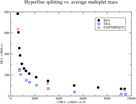
Figure 1: Hyperfine splitting versus spin averaged meson multiplet mass.

It is insightful to contrast this with non-relativistic quark model treatments which use a constituent quark mass about half the multiplet average and describe the splitting as a $1/\mathcal{M}^{2}$ dependence characteristic of relativistic corrections. Because the quarkonium Bohr orbit scales inversely with quark mass, it is possible for these models to describe both light and heavy meson splittings with the same short ranged hyperfine potential although it does require tuning of parameters. Indeed as Ref. gi details, a comprehensive meson description can be obtained by using a potential with a complicated, mass dependent short ranged smearing. Alternatively, the RPA-BCS formalism, which dynamically generates a constituent mass, reproduces this behavior via chiral symmetry and a simpler, weaker hyperfine interaction. The TDA, which also incorporates the same quasiparticle/constituent running masses as the RPA, in general provides a qualitatively comparable spin splitting description except for the $\pi$-$\rho$ difference. Of course by increasing the hyperfine strength it would be possible for the TDA to account for the large $\pi$-$\rho$ splitting, however, this enhanced interaction would then generate an overprediction for the $\pi^{\prime}$-$\rho^{\prime}$ and other splittings. For a comprehensive description the TDA would most likely require a more complicated hyperfine interaction with tuning and in this sense shares the same difficulties as constituent, non-chiral models mentioned in the introduction. The attractive feature of the RPA-BCS approach is the ability to obtain a good description with minimal parameters which is a common goal in all approaches to QCD and hadron structure.

Application to the isoscalar hyperfine splitting is not possible without a proper $\eta$-$\eta^{\prime}$ mixing calculation. However, using the strange current mass of 25 MeV and the preferred potential, model 4, the splitting for the pure $s\overline{s}$ mesons is 300 MeV, corresponding to a pseudoscalar mass of 720 MeV and a $\phi$ meson at 1020 MeV. The extracted strange constituent mass was 192 MeV. As the physical $\eta$ and $\eta^{\prime}$ masses are respectively 547 and 958 MeV, mixing effects are significant and it will be of interest to see the importance of the hyperfine interaction in a rigorous mixing analysis.

In addition to an improved meson spin spectrum, three of the model hyperfine interactions markedly increase the quark condensate which previous analyses orsay ; LC1 ; LC2 ; ls2 predicted too low, around $\langle\bar{q}q\rangle=-(110\ {\rm MeV})^{3}$. This was also noted in Ref. aspk . For models 2, 3 and 4 the new condensate varies between $-(165\ {\rm MeV})^{3}$ and $-(200\ {\rm MeV})^{3}$ in the chiral limit, a noticeable improvement but still below accepted values spanning the interval between $-(220\ {\rm MeV})^{3}$ and $-(260\ {\rm MeV})^{3}$. The pion decay constant, $f_{\pi}$, also improves but only marginally. These shifts are in the correct direction, as first noted by Alkofer and Lagaë Lagae , but complete agreement in this model is not possible without generating very large self energies which distort the meson spectrum. Because the decay constant is a matrix element connecting the ground state (model vacuum), the low calculated values also reflect shortcomings with the BCS vacuum. As detailed in Ref. LC2 the use of the superior RPA vacuum significantly increases $f_{\pi}$ (although not quite to the physical value). It would therefore be interesting to repeat this hyperfine calculation with an improved vacuum.

Naively, it is expected that the transverse potential should, as in the quantum mechanical quark model, decrease the mass of pseudoscalar states. However, it is important to distinguish between level splitting and absolute level shifts. The hyperfine interaction does indeed provide a level splitting with difference proportional to hyperfine strength, but it also increases the quasiparticle self-energy and thus the effective constituent quark mass as well. Consequently, both pseudoscalar and vector meson masses increase which then in turn requires a reduction in the current quark mass to reproduce the observed spectra.

This reduction in current quark mass was also necessary to describe states in bottomonium. The reported but unconfirmed $\eta_{b}$ state has a mass of 9300 MeV RPP , clearly below predictions (see Table 2) which are closer to non-relativistic perturbative QCD (NRPQCD) and lattice calculations pqcd that predict a much smaller $\Upsilon$-$\eta_{b}$ splitting of about 40 MeV with an error of about 20 to 30 MeV. A recent paper bak lowers this error to 10 (th$)^{+9}_{-8}$ ($\delta\alpha_{s}$) MeV reflecting uncertainties in theory and the strong coupling constant. The NRPQCD calculations, in particular, suffer from uncertainty in nonperturbative corrections that are usually parameterized in terms of condensates. Hence model calculations are still needed and the RPA predicts a splitting in rough agreement, but somewhat larger, than these theoretical expectations. Interestingly, the structure of the coupling (see Eqs. (35), (36) and (37)) is such to increase the splitting from the TDA value of around 20 MeV to the RPA prediction of 60 MeV. Although this is a minimal, secondary effect when compared to the absolute mass scale involved, it is still important for the relatively small hyperfine separation. This analysis therefore predicts that the $\eta_{b}$ meson mass should be around 9400 MeV and new results from spectroscopic studies at the B-factories are eagerly awaited.

III.2 Comparison to other hadronic approaches

It is instructive to make contact with alternative formulations and to further discuss the smaller current and constituent quark masses in our model. It is well known that a running current quark mass emerges in one loop QCD and values can be extracted at the perturbative $M_{Z}$ scale. Usually quoted, however, are their values at a much lower renormalization point such as 2 GeV in the $\overline{MS}$ scheme. While the ”experimental” bare quark values listed in Table 2 are obtained from measurement, they rely on significant model input either from chiral perturbation theory, as in the case of the $u$, $d$, $s$ masses, or from heavy quark effective theory for the $c$, $b$ quarks. They are thus not directly observable and entail both uncertainty and also ambiguity creutz . It is therefore more appropriate to regard them as parameters in the Lagrangian (Hamiltonian), subject to renormalization. Since our model kernel has been previously renormalized the only remnant of current quark mass running is the momentum dependence of the dressed quark mass $M_{q}(p)$. Effectively, the current quark renormalization point dependence has been converted into a constituent mass momentum dependence analogous to the Schwinger-Dyson treatment. Therefore when comparing to current masses from other approaches one should use the constituent running mass evaluated at the alternative model’s current mass scale, e.g. $M_{q}(p=2$ GeV), and not the smaller $m_{q}$ parameter appearing in our Hamiltonian. Figure 2 plots the running dependence of our model 4 dressed quark masses for different flavors. As this figure indicates at $p$ = 2 GeV, the scaled effective current quark masses are still lower than in other approaches, however they are much larger than our bare Hamiltonian values and provide a more realistic comparison. Related, the larger constituent masses in conventional quark models (ranges listed in Table II under ”experiment”) partially reflects missing dynamics from field theoretical self-energies that we explicitly include. The validity of any quark approach should consequently be judged more by the robustness of observable prediction (e.g. spectrum) rather than specific quark values. This is the case in the present analysis as indicated in Table 2, where the resulting quark masses are small when compared to the typically quoted values but the predicted meson masses are reasonable. We submit these smaller current quark values are representative of this simple, minimal parameter approach because the masses were uniformly small for all four, markedly different hyperfine interactions. An improved, rigorous treatment entailing a complicated combined quark-gluon sector diagonalization of the exact hyperfine Hamiltonian, Eq. (7), is in progress which will firmly ascertain if small quark values are required.

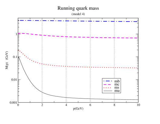
Figure 2: Constituent $u/d$, $s$, $c$ and $b$ running quark masses from Eq. (29).

Finally, predictions for the “J parameter”

$$J=M_{R}{dM_{V}\over dM_{Ps}^{2}}$$ (48)

are presented which has been proposed as a reliability measure for quenched lattice computations of light hadron masses J . Here $M_{Ps}$, $M_{V}$ are the pseudoscalar, vector meson masses and $M_{R}$ is the (reference) vector mass determined by the intersection of the line $M_{V}=1.8\ M_{Ps}$ with the plot of $M_{Ps}^{2}$ versus $M_{V}$. If the vector meson mass is linear in the current quark mass and, as indicated by Eq. (3), the pseudoscalar scales as the square root, then a sensitive lattice chiral extrapolation is not required to evaluate $J$ and the attending errors can be avoided. Results from unextrapolated quenched lattice simulations J predicts $J=0.37$ which should be contrasted with the estimate $J=0.48$ using the physical $\pi$, $\rho$, $K$ and $K^{*}$ masses. The difference reflects the need to include dynamical fermions in the lattice calculations.

Figure 3: Determining the $J$ parameter. The solid curve corresponds to $M_{V}=1.8\ M_{Ps}$ while the other lines are linear fits to the TDA and RPA predictions.

Figure 3 shows the TDA and RPA masses and the curve $M_{V}=1.8\ M_{Ps}$. As anticipated, the RPA points scale linearly and extrapolate to zero pion mass at a vector mass of approximately 780 MeV. A linear fit to the RPA gives a reference mass of $M_{R}=880$ MeV and $J=0.42$, in more reasonable agreement with the estimate from data. Surprisingly, the TDA points also scale linearly even though they do not yield a zero mass pion in the chiral limit. This lowers the reference vector mass and produces a $J$ parameter of $0.36$. It will prove instructive to confront these predictions with dynamical quark lattice simulations especially those using realistic sea quark masses.

IV Conclusion

As a consequence of this study, the relative importance of chiral symmetry and the hyperfine interaction is clearer: spin splittings in heavy quark systems are not governed by chiral symmetry and only require a hyperfine interaction. However, for light mesons chiral symmetry is important and is essential for describing the $\pi$-$\rho$ mass difference in a minimally parameterized, heavily constrained model such as the one advocated here. Indeed the RPA-BCS many-body approach provides a reasonable description of the pseudoscalar-vector spectrum for both light and heavy mesons with a common Hamiltonian containing only the current quark masses and two dynamical parameters. By explicitly incorporating this important symmetry of QCD, a small pion mass is dynamically generated without the necessity of tuning a complicated hyperfine potential as typically done in conventional quark models. Furthermore, including a hyperfine interaction in this many-body approach improves both the pion decay constant and the quark condensate predictions which previously have been calculated too low. The hyperfine interaction also enhances the self energy contribution to the quark kinetic energy which necessitates using much smaller current quark masses. Lastly, the RPA $J$ parameter is closer to data than quenched lattice results and it will be interesting to compare with dynamical quark lattice simulations.

Future work includes reanalyzing the glueball, meson and hybrid spectra with the hyperfine potential and examining other short range interactions such as the tensor, $\alpha_{i}\alpha_{j}$ - $\alpha_{i}\alpha_{j}$, and higher dimensional terms from excluded Fock space components Bicudo3 . Extensions of this approach to highly excited hadron states will also be of interest, based upon the need ess2 for new relativistic, chirally invariant models with a nontrivial vacuum. Finally, investigations of baryons should also be fruitful as previous non-hyperfine calculations L2 only predict about half of the observed $N$-$\Delta$ splitting.

- (1) See, for example, D.J. Griffiths, Introduction to Elementary Particles (John Wiley & Sons, Inc., 1987).
- (2) S. Godfrey and N. Isgur, Phys. Rev. D 32, 189 (1985).
- (3) S. Capstick and N. Isgur, Phys. Rev. D 34, 2809 (1986).
- (4) A.P. Szczepaniak and E.S. Swanson, Phys. Rev. D 65, 025012 (2002); Phys. Rev. D 62, 094027 (2000).
- (5) R. Delbourgo and M.D. Scadron, J. Phys. G 5, 1621 (1979).
- (6) A. Bender, C.D. Roberts and L.v. Smekal, Phys. Lett. B 380, 7 (1996).
- (7) P. Maris, C.D. Roberts and P.C. Tandy, Phys. Lett. B 420, 267 (1998).
- (8) See recent review and references therein by P. Maris and C.D. Roberts, Int J. Mod. Phys. E 12, 297 (2003).
- (9) E.S. Swanson, in Proceedings of the Workshop on the Physics of Excited Nucleons, edited by S.A. Dytman and E.S. Swanson (World Scientific, Hong Kong, 2003), p. 157.
- (10) J.R. Finger and J.E. Mandula, Nucl. Phys. B199, 168 (1982); S.L. Adler and A.C. Davis, Nucl. Phys. B244, 469 (1984); A. Le Yaouanc, L. Oliver, S. Ono, O. Pene and J.C. Raynal, Phys. Rev. D 31, 137 (1985).
- (11) A.P. Szczepaniak, E.S. Swanson, C.R. Ji and S.R. Cotanch, Phys. Rev. Lett. 76, 2011 (1996).
- (12) F.J. Llanes-Estrada, S.R. Cotanch, P. Bicudo, E. Ribeiro and A. Szczepaniak, Nucl. Phys. A710, 45 (2002).
- (13) A.P. Szczepaniak and E.S. Swanson, Phys. Lett. B 577, 61 (2003).
- (14) E.S. Swanson and A.P. Szczepaniak, Phys. Rev. D 59, 014035 (1999).
- (15) F.J. Llanes-Estrada and S.R. Cotanch, Phys. Lett. B 504, 15 (2001).
- (16) F.J. Llanes-Estrada and S.R. Cotanch, Phys. Rev. Lett. 84, 1102 (2000).
- (17) F.J. Llanes-Estrada and S.R. Cotanch, Nucl. Phys. A697, 303 (2002).
- (18) N. Ligterink and E. S. Swanson, Phys. Rev. C 69, 025204 (2004) [arXiv:hep-ph/0310070].
- (19) A.P. Szczepaniak and E.S. Swanson, Phys. Rev. D 55, 1578 (1997).
- (20) D.G. Robertson, E.S. Swanson, A.P. Szczepaniak, C.R. Ji and S.R. Cotanch, Phys. Rev. D 59, 074019 (1999).
- (21) A.P. Szczepaniak and E.S. Swanson, Phys. Rev. Lett. 87, 072001 (2001).
- (22) A.P. Szczepaniak and P. Krupinski, Phys. Rev. D 66, 096006 (2002).
- (23) J.E. Villate et al., Phys. Rev. D 47, 1145 (1993); P. Bicudo et al., Phys. Rev. D 45, 1673 (1992).
- (24) P. Bicudo and J. Ribeiro, Z. Phys. C 38, 454 (1988); Phys. Rev. D 42, 1611 (1990).
- (25) S.-K. Choi et al. (Belle Collaboration), Phys. Rev. Lett. 89, 142001 (2002).
- (26) R. Alkofer and P.A. Amundsen, Nucl. Phys. B306, 305 (1988); J.-F. Lagaë, Phys. Rev. D 45, 317 (1992).
- (27) K. Hagiwara et al., Phys. Rev D 66, 010001 (2002).
- (28) A. Pineda and F.J. Yndurain, Phys. Rev. D 61, 077505 (2000); C. T. H. Davies et al. [UKQCD Collaboration], Phys. Rev. D 58, 054505 (1998) [arXiv:hep-lat/9802024].
- (29) B.A. Kniehl et al., hep-ph/0312086.
- (30) M. Creutz, hep-ph/0312225.
- (31) P. Lacock and C. Michael, Phys. Rev. D 52, 5213 (1995).
- (32) E. S. Swanson, Phys. Lett. B 582, 167 (2004) [arXiv:hep-ph/0309296].
- (33) F.J. Llanes-Estrada, unpublished.