We present a unique parameterization of the equation of state of strongly interacting matter in the temperature interval $0.6T_{c}\cdots 3T_{c}$ at $\mu=0$ within a quasi-particle model based on quark and gluon degrees of freedom. The extension to non-vanishing baryon-chemical potential is discussed.

1 Introduction

The equation of state (EoS) of strongly interacting matter contains important information about bulk properties and the thermodynamics. In fact, one needs the EoS as input for describing hydrodynamically the evolution of the early universe, dynamics and static characteristics of neutron stars as well as certain stages of relativistic heavy-ion collisions. Considerable progress has been achieved during the last years in calculating the EoS from first principles resting on quantum chromodynamics (QCD). By advanced sampling techniques the EoS of strongly interacting matter is numerically accessible from lattice QCD calculations. Many details have been considered for particle-antiparticle symmetric matter. Here, at a certain value of the temperature, $T_{c}$, the susceptibilities corresponding to the Polyakov loop and the chiral condensate display pronounced peaks indicating deconfinement and chiral symmetry restoration (cf. [1]). Above $T_{c}$, in the deconfinement region, the relevant degrees of freedom of strongly interacting matter are thought to be quarks and gluons. Despite asymptotic freedom, in the range of $T_{c}<T<2.5T_{c}$, the EoS behaves highly non-trivial, preventing a direct perturbative treatment. There are various attempts to understand the EoS in this range and above, such as dimensional reduction, resummed HTL scheme, $\Phi$ functional approach, Polyakov loop model etc. (cf. [2] for a recent survey). A controlled chain of approximations from full QCD to some analytical expressions describing the lattice data without adjustable parameters would be of desire. Success has been achieved for $T>2.5T_{c}$ [3]. In contrast, the range $T>T_{c}$, in particular near to $T_{c}$, is covered by phenomenological models [4, 5, 6, 7] with parameters adjusted to lattice QCD data.

Below $T_{c}$, in the confinement region, hadrons are thought to be the relevant degrees of freedom. Detailed information about the EoS in this range from lattice QCD became available very recently [8], offering a chance to check phenomenological models for the first time. In [9] lattice QCD data from [8] for $T<T_{c}$ have been shown to agree with results of a hadron resonance gas model including a large number of states up to 2 GeV. Taking a different point of view, we present here a description of the lattice QCD data [8] in the range $0.6T_{c}<T<3T_{c}$ by our quasi-particle model of quarks and gluons [4, 5]. Up to now it has been proven that our model can reproduce lattice data in the range $T_{c}\cdots 3T_{c}$ for the pure gluon plasma [4] and for quark-gluon plasmas with various quark-flavor numbers [5]. Here, our focus is to cover the lattice QCD data in the confinement region.

Our paper is organized as follows. In section 2 we recapitulate features of our quasi-particle model. The comparison with lattice QCD data at vanishing chemical potential is performed in section 3. We discuss the obtained parameterization of the equation of state in section 4. Section 5 is devoted to non-vanishing chemical potential. The summary can be found in section 6.

2 Quasi-particle Model

Our quasi-particle model of light and strange quarks ($q,s$) and gluons ($g$) is based on the entropy density

$$s=\sum_{i=q,s,g}s_{i},\,s_{i}=\frac{d_{i}}{2\pi^{2}T}\int dkk^{2}\left[\frac{\left(\frac{4}{3}k^{2}+m_{i}^{2}\right)}{\sqrt{m_{i}^{2}+k^{2}}}(f_{+}(k)+f_{-}(k))-\mu(f_{+}(k)-f_{-}(k))\right]$$ (1)

and the quark number density

$$n=\frac{d_{q}}{2\pi^{2}}\int dkk^{2}\left[f_{+}(k)-f_{-}(k)\right]$$ (2)

with degeneracies $d_{q}=12$, $d_{s}=6$ and $d_{g}=8$ as for free partons, and distribution functions $f_{\pm}(k)=(\exp([\sqrt{m_{i}^{2}+k^{2}}\mp\mu]/T)+S)^{-1}$ with $S=+1$ ($-1$) for quarks (gluons). The chemical potential is $\mu$ for light quarks and anti-quarks, respectively, while $\mu=0$ for strange quarks and gluons. The parton effective masses

$$m_{i}^{2}(T,\mu)=m_{i,0}^{2}+\Pi_{i}(k;T,\mu)$$ (3)

have a rest mass contribution $m_{i,0}^{2}$ and, as essential part, the one-loop self-energies at hard momenta $\Pi_{i}(k;T,\mu)$. The crucial point is to replace in $\Pi_{i}(k;T,\mu)$ the running coupling by an effective coupling, $G^{2}(T,\mu)$ [4]. (As shown in [10], it is the introduced modification of $G^{2}(T,\mu)$ which allows to describe the lattice QCD data, while the use of the 1-loop or 2-loop perturbative coupling together with a more complete description of the plasmon term and Landau damping restricts the approach to $T\geq 2.5T_{c}$.) In doing so, non-perturbative effects are thought to be accommodated in this effective coupling. In massless $\Phi^{4}$ theory such a structure of the entropy density emerges by resumming the super-daisy diagrams in tadpole topology [11], and [12] argues that such an ansatz is also valid for QCD. [3] point to more complex structures, but we find (1, 2) flexible enough to accommodate the lattice data (see below).

The pressure reads accordingly

$$p=\sum_{i=q,s,g}p_{i}-B(T,\mu),\quad p_{i}=\frac{d_{i}}{6\pi^{2}}\int dk\frac{k^{4}}{\sqrt{m_{i}^{2}+k^{2}}}\left[f_{+}(k)+f_{-}(k)\right],$$ (4)

where $B(T,\mu)$ ensures thermodynamic self-consistency, $s=\partial p/\partial T$, $n=\partial p/\partial\mu$ together with the stationarity condition $\delta p/\delta m_{i}^{2}=0$ [13]. Note that eqs. (1, 2, 4) themselves are highly non-perturbative expressions: Expanding (4) in powers of the coupling strength one recovers the first perturbative terms. (Higher order terms would probably need higher orders in $\Pi$). For more details on our model see [4, 5, 6, 10, 12].

3 Comparison with lattice data at ${\bf\mu=0}$

(1) represents a mapping of lattice data for $s(T)$ on $G^{2}(T)$; to determine $p$ one has to fix an integration constant, say $B(T_{c})$. As in the lattice calculations [8] we have used $m_{i,0}=x_{i}T$ with $x_{q}=0.4$ for light quark flavors, $x_{s}=1$ for strange quarks and $x_{g}=0$. We have found as a convenient parameterization

$$G^{2}(T)=\left\{\begin{array}[]{l}G^{2}_{\rm 2-loop},\quad T\geq T_{c}\\[8.53581pt] a-bT/T_{c},\quad T<T_{c}\end{array}\right.$$ (5)

where $G^{2}_{\rm 2-loop}$ is the 2-loop coupling

$$G^{2}_{\rm 2-loop}=\frac{16\pi^{2}}{\beta_{0}\log\xi^{2}}\left[1-\frac{2\beta_{1}}{\beta_{0}^{2}}\frac{\log(\log\xi^{2})}{\log\xi^{2}}\right]$$ (6)

with $\beta_{0}=(11N_{c}-2N_{f})/3$, $\beta_{1}=(34N_{c}^{2}-13N_{f}N_{c}+3N_{f}/N_{c})/6$, and the argument $\xi=\lambda(T-T_{s})/T_{c}$. The parameters are $T_{s}=0.80T_{c}$, $\lambda=7.6$, $a=359.0$ and $b=334.5$ for $N_{f}=2+1$, $N_{c}=3$. The comparison of our model with the lattice data [8, 9] is exhibited in Fig. 1 by solid curves for entropy density and pressure, respectively. One observes an impressively good description of the lattice data, in particular also below $T_{c}$.

Remarkable is the change of the shape of $G^{2}(T)$ at $T_{c}$, see Fig. 2. Above $T_{c}$, $G^{2}(T)$ resembles the usual 2-loop running coupling strength with a regulator $T_{s}$, which ensures agreement with the data down to $T_{c}$. Going down in $T$, at $T_{c}$ the growing of $G^{2}(T)$ is changed into a moderate linear rise. Note that no order parameter is needed which changes at $T_{c}$. This is possibly related to the fact that $s$ is a measure for the density of states. Also, the degeneracies $d_{i}$ are constant.

Here we would like to contrast our quasi-particle model based on quark-gluon degrees of freedom with the resonance gas model below $T_{c}$ [9]. The authors of [9] state that many heavy resonances are needed to describe the data (at $T_{c}$ the lightest hadron contribution to the energy density is at the level of $15\%$ [9]). Our result is in some correspondence, in the sense that fairly heavy quasi-particle excitations are needed which emerge from the large values of $G^{2}$. One could also argue that a large number of excited hadron states at $T<T_{c}$ can be effectively described in an equivalent manner by a small number of quasi-particle excitations, as we do here.

It is well conceivable that, for determining the pressure (4), two distinct integration constants would be needed, say $B(T_{c}^{+})$ and $B(T_{c}^{-})$. However, one constant $B(T_{c})=0.44T_{c}^{4}$ is sufficient to describe the pressure, see right panel in Fig. 1.

As mentioned above, the lattice calculations [8] use quite heavy quarks. A possible estimate of the chiral extrapolation is to put $m_{i,0}=0$ and repeat the evaluation of eqs. (1 - 4) with keeping the parameters in (5) fixed; $B(T_{c})$ is adapted to ensure a positive pressure. The results are shown as dashed curves in Fig. 1. Such a procedure is certainly too simple. Only once lattice results for various $m_{i,0}$ are at our disposal one can estimate the $m_{i,0}$ dependence of the parameters in (5) and for $B(T_{c})$ to achieve a more profound chiral extrapolation.

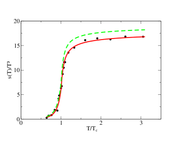
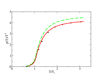
Figure 1: Entropy density $s$ scaled by $T^{3}$ (left panel) and pressure scaled by $T^{4}$ (right panel) as a function of the temperature in units of the pseudo-critical temperature $T_{c}$. The full (dashed) curves represent calculations with lattice masses as described in text ($m_{i,0}=0$ as an estimate of the chiral extrapolation). Lattice data from [8, 9].

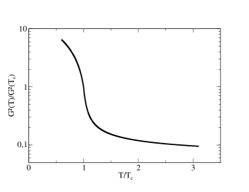
Figure 2: The effective coupling $G^{2}(T)$ (in units of $G^{2}(T_{c})$) as a function of the temperature.

4 Discussion

Up to this point we consider eqs. (1 - 4) as a convenient unique parameterization of the EoS, which one may make use of for purposes mentioned in the introduction. Further detailed lattice data are needed to test our model at even smaller temperatures and to see where an explicit change to hadronic degrees of freedom is required.

In an restricted interval around $T_{c}$ one may speculate whether a quark-hadron duality is at work, i.e. hadron observables are expressed in a quark-gluon basis and vice versa. For example, [9] shows that in a narrow interval above $T_{c}$ the hadron resonance gas model still agrees with the lattice data. Above $T_{c}$, signals of hadronic states have been found as well [14], an aspect advocated as important in [15]. Even more, [16] has shown that a modified resonance gas model describes the lattice data above $T_{c}$ also successfully.

There are various examples of the quark-hadron duality in the literature. We mention here QCD sum rules [17] which realize the duality, as discussed in [18]. Another observation is that in heavy-ion collisions the low-mass di-electron spectra can be described by a quark-gluon plasma emission rate, even if the space-time averaged temperature of the emitting system is below $T_{c}$ [19]. For further aspects of the duality we refer, e.g., to [20].

5 Non-vanishing chemical potential

With the advent of lattice QCD data at non-vanishing chemical potential [21, 22, 23] the equation of state becomes accessible in a large region. This is particularly important as the envisaged CBM project at the future accelerator complex in Darmstadt [24] aims at exploring systematically the region of maximum baryon densities at reach in heavy-ion collisions.

As described in [6, 12] our quasi-particle model also covers the equation of state for non-vanishing chemical potential. The point here is that thermodynamical self-consistency allows to map the lattice QCD data from $\mu=0$ to $\mu>0$ without further assumptions. Indeed, as shown in [25] our model agrees quite perfectly with lattice QCD calculations at $\mu>0$ for $2+1$ flavors. Here we focus on the recent lattice QCD data for 2 flavors [23] with improved p4 action. Given $G^{2}(T)$ (e.g., from the previous section, or from an analysis of other lattice QCD data such as [23]) as boundary values, the partial differential equation $a_{T}\partial G^{2}(T,\mu)/\partial T+a_{\mu}\partial G^{2}(T,\mu)/\partial\mu+a_{T,\mu}=0$ with $a_{T}(\mu=0)=0$ and $a_{\mu}(T=0)=0$ (cf. [6, 12] for details) delivers as solution $G^{2}(T,\mu)$, needed in $\Pi_{i}(k;T,\mu)$. Fig. 3 exhibits the characteristic curves for solving this ”flow equation”. Asymptotically, $G^{2}$ is constant along the characteristic curves. As discussed in [6, 12] we take the characteristic curve emerging from $T_{c}$ at $\mu=0$ (solid curve in Fig. 3) as indicator of the phase border line. It agrees up to intermediate values of $\mu$ fairly well with estimates based on lattice QCD calculations [22]. The characteristic curves above the solid curve show a regular pattern of sections of ellipses. In contrast, the characteristic curves emerging from the $T$ axis below $T_{c}$ are flatter and cross the former ones at larger values of $\mu$. This may indicate that the model is not longer applicable in that region. To understand the pattern of the characteristic curves we note that, in the region of interest, the characteristic curves have a universal shape, i.e., for small values of $\mu$ the shape is independent of the actual start value $G^{2}(T,\mu=0)$. For sufficiently small values of $G^{2}(T,\mu=0)$, the characteristic curves form a nested set of non-intersecting ellipse like curves. Increasing $G^{2}(T,\mu=0)$ causes a levelling-off at larger values of $\mu$. The levelling-off sets in at smaller values of $\mu$ for larger values of $G^{2}(T,\mu=0)$. This causes the pattern seen in Fig. 3.

Having $G^{2}(T,\mu)$ at our disposal, the EoS follows from eqs. (1 - 4) in a straightforward way. Fig. 4 shows as example a comparison of our model with the lattice QCD data from [23] for $N_{f}=2$. Again, a fairly well reproduction of the data is achieved for $T>T_{c}$, while at $T<T_{c}$, in particular for large values of $\mu$, the agreement is less perfect.

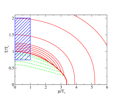
Figure 3: The characteristic curves solving the flow equation for the effective coupling $G^{2}$. Solid (dashed) lines: characteristic curves emerging from $T>T_{c}$ ($T<T_{c}$). The heavy solid curve is considered as indicator of the phase border line. The characteristic curves are not drawn in the region where they intersect. The marked region indicates where the lattice QCD data [23] are given. Note that they are actually provided by the truncated expansion $\Delta p/T^{4}\equiv p(T,\mu=0)/T^{4}-p(T,\mu)/T^{4}=c_{2}(T)(\mu/T)^{2}+c_{4}(T)(\mu/T)^{4}$. Higher order terms, like $c_{6}(T)\,(\mu/T)^{6}$ etc. are needed to control the validity of the extrapolation to larger values of $\mu$.

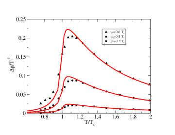
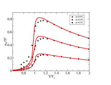
Figure 4: The scaled pressure difference $\Delta p(T,\mu)=p(T,\mu)-p(T,\mu=0)$ (left panel) and the scaled quark number density (right panel) as a function of the temperature for various chemical potentials. Data from [23].

6 Conclusions

To summarize, we present a unique parameterization of the equation of state of strongly interacting matter in the temperature interval $0.6T_{c}\cdots 3T_{c}$ which is based on the picture of weakly interacting quasi-particles of quarks and gluons. At $T_{c}$ for $\mu=0$, the temperature dependence of the effective coupling suffers a change; no rapidly changing order parameter is needed to describe the lattice QCD data. Further precision lattice data below $T_{c}$ are needed to check the model in more detail and to put the speculation on firm ground, such that the applicability of the quasi-particle picture provides an additional example of quark-hadron duality.

It has been shown that our model is also able to describe the new lattice QCD data for non-vanishing chemical potential, as alternative approaches do [26, 27]. As particular new point we note that we cover the region $T<T_{c}$ at non-vanishing but small chemical potential with our quasi-particle model.

While present lattice QCD data deliver either $p(T,\mu=0)$ or $\Delta p(T,\mu)$, our model covers both quantities on the same footing.

Inspiring discussions with J.P. Blaizot, D. Blaschke, A. Peshier, and K. Redlich are gratefully acknowledged. The work is supported by BMBF 06DR121, GSI and FP6-I3 network.

References

- [1] F. Karsch, Lect. Notes Phys. 583, 1 (2002)
- [2] D.H. Rischke, nucl-th/0305030
-
[3]
J.P. Blaizot, E. Iancu, A. Rebhan, Phys. Rev. Lett. 83, 2906 (1999);
Phys. Lett. B470, 181 (1999); Phys. Rev. D63, 065003 (2001);
68, 025011 (2003), hep-ph/0303185
J.O. Andersen, E. Braaten, M. Strickland, Phys. Rev. Lett. 83, 2139 (1999); Phys. Rev. D61, 014017 (2000), 63, 105008 (2001)
P. Romatschke, hep-ph/0210331 - [4] A. Peshier, B. Kämpfer, O.P. Pavlenko, G. Soff, Phys. Lett. B 337, 235 (1994); Phys. Rev. D 54, 2399 (1996)
- [5] A. Peshier, B. Kämpfer, G. Soff, Phys. Rev. C 61, 045203 (2000)
- [6] A. Peshier, B. Kämpfer, G. Soff, Phys. Rev. D 66, 094003 (2002)
-
[7]
P. Levai, U. Heinz, Phys. Rev. C 57, 1879 (1998);
R.A. Schneider, W. Weise, Phys. Rev. C 64, 055201 (2001);
A. Rebhan, P. Romatschke, Phys. Rev. D 68, 025022 (2003) - [8] F. Karsch, E. Laermann, A. Peikert, Nucl. Phys. B 605,579 (2001); Phys. Lett. B 478, 447 (2000)
- [9] F. Karsch, K. Redlich, A. Tawfik, Eur. Phys. J. C 29, 549; Phys. Lett. B 571, 67 (2003)
- [10] A. Peshier, B. Kämpfer, G. Soff, hep-ph/0312080
- [11] A. Peshier, B. Kämpfer, O.P. Pavlenko, G. Soff, Eur. Phys. Lett. 43, 381 (1998)
- [12] A. Peshier, hep-ph/9910451, Phys. Rev. D 63, 105004 (2001)
- [13] M.I. Gorenstein, S.N. Yang, Phys. Rev. D 52, 5206 (1995)
- [14] C. DeTar, J.B. Kogut, Phys. Rev. D 36, 2828 (1987)
- [15] E. Shuryak, I. Zahed, hep-ph/0307267
- [16] D.B. Blaschke, K.A. Bugaev, nucl-th/0311021
- [17] M.A. Shifman, A.I. Vainshtein, V.I. Zakharov, Nucl. Phys. B 147, 448 (1979)
- [18] T.D. Cohen, R.J. Furnstahl, D.K. Griegel, X. Jin, Prog. Part. Nucl. Phys. 35, 221 (1995)
- [19] K. Gallmeister, B. Kämpfer, O.P. Pavlenko, C. Gale, Nucl. Phys. A 698, 424 (2002)
-
[20]
Y.B. Dong, M.F. Li, Phys. Rev. C 68, 015207 (2003)
Q. Zhao, F.E. Close, Phys. Rev. Lett. 91, 022004 (2003) - [21] Z. Fodor, S.D. Katz, K.K. Szabo, Phys. Lett. B 568, 73 (2003)
- [22] C.R. Allton et al., Phys. Rev. D 66, 074507 (2002)
- [23] C.R. Allton et al., Phys. Rev. D 68, 014507 (2003)
- [24] see http://www.gsi.de/documents/DOC-2004-Jan-116-1.pdf for the Letter of Intend of the Compressed Baryon Matter (CBM) project
- [25] K.K. Szabo, A.I. Toth, JHEP 0306, 008 (2003)
- [26] M.A. Thaler, R.A. Schneider, W. Weise, hep-ph/0310251
- [27] J. Letessier, J. Rafelski, Phys. Rev. C 67, 031902 (2003)