Preprint HNINP-V-04-02
Observables with $\tau$ leptons at LHC and LC
structure of event records and Monte Carlo Algorithms

Abstract

In the present report, let us adress the issues related to simulation of decays for particle embodied in full production and decay chains of Monte Carlo programs set-up for experiments such as at LHC or LC. Both technical issues related to the way how the events may be stored in event records and issues related to physics (in particular non-factorizable correlations of the Einstein-Rosen-Podolsky type) will be reviewed on the basis of practical examples. We will limit our discussion to the case of $\tau$ lepton and $W$ boson decays, but similar problems (and solutions) may arise also in case of simulation for other intermediate states or particles. Examples related to construction of physics observables will be also given. In particular the method of measuring the CP parity properties of the $h-\tau\tau$ coupling at LC will be explained.

Presented at IX Workshop on A C A T in Physics Research, December 1-5, 2003, KEK, Tsukuba, Japan

1 Introduction

Since many years, intensive studies are being performed to design future software architectures for experiments on proton proton colliders, such as the Tevatron or the LHC [1] and high energy $e^{+}e^{-}$ linear colliders such as JLC, NLC [2] or TESLA [3].

One of the important ingredients in such designs is the data structure for storing the Monte Carlo events. It is generally accepted that the data structures based on objects such as particles, clusters, strings, etc. with properties such as tracks, momenta, colour, spin, mass, etc. and on the relations explaining the origins and descendants of the objects is the most convenient one. This is the case at present [4], and it is also envisaged for the future, see [5]. At the same time such a picture is in conflict with the basic principles of quantum mechanics. Einstein–Rosen–Podolsky paradox is an example of such phenomena. A general problem is that the quantum state of a multiparticle system cannot (at least in principle) be represented as a statistical combination of the states defined by the products of the pure quantum states of the individual particles. It is thus of the utmost importance to examine whether the approximation enforced by the data structure is purely academic, or if it rather represents a real difficulty, which may affect the interpretation of the future data. In fact in some cases alternative methods can be designed and are in fact used as well.

It would not be a serious problem if the predictions of the Standard Model used in the interpretation of the future data could be provided by a single program, black box, without any need of analysing its parts. Then anything that would be measured beyond the prediction of such a hypothetical Monte Carlo program would be interpreted as “new physics”. Agreement, on the other hand, would constitute confirmation of the Standard Model, as it is understood at present (and proper functioning of the detector as well). However, even in such an extreme case it is very useful, for the purpose of experimental studies, to manipulate with the terms responsable for the signature of the ‘new physics’. In this way experimental strategies can be refined, if the new effects can be placed in well defined and phenomenologically simple modules.

Because of the complexity of the problem, Monte Carlo predictions need to be dealt with by programs describing: the action of the detector and of the analysis, on the experimental side, and various effects, such as those from hard processes, hadronization, decay of resonances, etc., on the theoretical side. Every part is inevitably calculated with some approximation, which need to be controlled.

2 Event record and decay interface

In the first part I will discuss solution we used in KORALZ [6] – the program widely used at LEP for the simulation of $\tau$-lepton pair production and decay, including spin and QED bremssstrahlung effects. Even though spin effects are non-treatable in the scheme where properties are attributed to individual particles only, it is the very method used there. As described in ref. [6] the algorithm of spin generation for any individual event was consisting of the following steps:

1. An event consisting of a pair of $\tau$ leptons, bremsstrahlung photons, etc., was generated.

2. Helicity states for both $\tau^{+}$ and $\tau^{-}$ were generated. At this point, an approximation with respect to quantum mechanisc was introduced.

3. Information on these helicty states, including the definition of quantization frames, i.e. the relation between $\tau$’s rest frame and laboratory frame, was then transmitted to TAUOLA [7, 8, 9], the package for the generation of $\tau$-lepton decays.

4. Finally TAUOLA performed decays of 100% polarized $\tau$’s, and the event in the HEPEVT common block was completed.

The solution for the spin treatment of $\tau$ leptons at LEP was optimal. On one side, a convenient picture of particles with properties, origins and descendants could be used and, on the other, a complete full spin solution [10, 11] was available, if necessary.

Let us now turn to another example of the spin implementation algorithm. It is taken from ref.[12]. The algorithm, essentially that of KORALZ, was adopted to work with any Monte Carlo program providing the production of $\tau$-leptons. If the generated events are stored in the format of a HEPEVT common block, then the algorithm consisting of the following basic steps can be used:

1. Search for $\tau$-leptons in a HEPEVT common block (filled by any MC program).

2. Check what the origin of $\tau$–lepton is: $Z,\gamma,W,h,H^{\pm}$ or eventually, $2\to 2$–body process such as: $e^{+}e^{-},\;(u\bar{u}),\;(d\bar{d})\to\tau^{+}\tau^{-}$.

3. For the $2\to 2$–body process of $\tau$-pair production, it is sometimes possible to calculate the $\tau$ polarization as a function of the invariant mass of the $\tau$–lepton pair and angle between the directions of $\tau$–leptons and incoming effective beams (in the rest frame of $\tau$-pair).

4. If in addition to the $\tau$-leptons, photons or partons (gluons, quarks, etc.) are stored in HEPEVT common block, one needs to define the “effective incoming beams”.

5. From such an information one can generate $\tau$ helicity states and define the relation between the $\tau$ rest frame and the laboratory frame. Optionally complete spin effects can be implemented as well, see [18].

6. The $\tau$ decay is generated with the help of TAUOLA and HEPEVT common block is appended with the $\tau$’s decay products.

Leading spin effects are nicely reproduced by the above set of programs. A more complete discussion can be found in ref. [12].

Figure 1: Typical relations in present day event record. Daughter index JDAHEP points upward in a tree, however mother index JMOHEP may point to the previous copy of the event as well. The status code ISTHEP is ocasionally used like a pointer toward higher level of the event record listing. As a consequence in the event record there may appear ambiguities and/or loops for searching algorithms.

Let us stress, that the presented above solution, require certain minimal discipline in a way how the event records are filled in. At present, there is a strong tendency to store in event record, not only information on the ‘real particles’, but also on the results of the simulation at the parton shower level as well as of the hard process alone. As a consequence not only the same entries for the otherwise well defined partilces like $\tau$-leptons are duplicated or even triplicated, but also the relation between different entries is not anymore of the tree-type and links between particles are not reversible. The link upwards from $A$ to $B$ does not mean that there is downward link from $B$ to $A$. This creates multitude of troubles for the algorithms analyzing events, see fig. 1. However at present our solution for interfacing decay packages with the host programs based on HEPEVT event record as filled by PYTHIA and HERWIG seem to work in all cases studied by us [13]. For the case of complete spin correlations, we found it more convenient to abandon direct use of spin information provided by the host programs. Instead we choose to calculate complete density matrix anew, from the kinematical configuration provided by the host program.

3 Higgs boson parity measurement

Let us sketch the basic principles behind the proposed measurement, in the case, when simultaneosly scalar and pseudoscalar couplings are allowed in $h\tau\tau$ vertex

$$h\;\bar{\tau}N(\cos\phi+i\sin\phi\gamma_{5})\tau.$$ (1)

If non-zero CP-odd admixture to the Higgs is present, the distribution of the Higgs production angle is modified [14, 15, 16]. We have simulated production angular distributions as in the SM, but this assumption has no influence on the validity of the analysis. In order to study the sensitivity of $h\to\tau^{+}\tau^{-}$ observables, we assume a SM production rate inependent of the size of the CP-odd admixture.

The production process $e^{+}e^{-}\to Zh\to\mu^{+}\mu^{-}(q\bar{q})\tau^{+}\tau^{-}$ has been chosen, as an representative example, and simulated with the Monte Carlo program PYTHIA 6.1 [17]. The Higgs boson mass of 120 GeV and a centre-of-mass energy of 350 GeV was chosen. The effects of initial state bremsstrahlung were included. For the sake of our discussion and in all of our samples the $\tau$ decays have been generated with the TAUOLA Monte Carlo library [9, 8, 7]. As usual, to facilitate the interpretation of the results, bremsstrahlung effects in decays were not taken into account. Anyway, with the help of additional simulation, we have found this effect to be rather small. To include the full spin effects in the $h\to\tau^{+}\tau^{-}$, $\tau^{\pm}\to\rho^{\pm}\bar{\nu}_{\tau}(\nu_{\tau})$, $\rho^{\pm}\to\pi^{\pm}\pi^{0}$ decay chain, the interface explained in Ref. [18] was used.

The Higgs boson parity information must be extracted from the correlations between $\tau^{+}$ and $\tau^{-}$ spin components, which are further reflected in correlations between the $\tau$ decay products in the plane transverse to the $\tau^{+}\tau^{-}$ axes [19, 20]. To better visualize the effect, let us write the decay probability, using the conventions of Ref. [15]:

$$\Gamma(h_{mix}\to\tau^{+}\tau^{-})\sim 1-s^{\tau^{+}}_{\parallel}s^{\tau^{-}}_{\parallel}+s^{\tau^{+}}_{\perp}R(2\phi)~{}s^{\tau^{-}}_{\perp},$$ (2)

where $R(2\phi)$ can be understood as an operator for the rotation by an angle $2\phi$ around the ${\parallel}$ direction. The $s^{\tau^{-}}$ and $s^{\tau^{+}}$ are the $\tau^{\pm}$ polarization vectors, which are defined in their respective rest frames. The symbols ${\parallel}$/${\perp}$ denote components parallel/transverse to the Higgs boson momentum as seen from the respective $\tau^{\pm}$ rest frames.

The method relies on measuring the acoplanarity angle of the two planes, spanned on $\rho^{\pm}$ decay products and defined in the $\rho^{+}\rho^{-}$ pair rest frame. The acoplanarity angle $\varphi^{*}$, between the planes of the $\rho^{+}$ and $\rho^{-}$ decay products is defined. The angle is defined first, with the help of its cosine and two vectors ${\bf n}_{\pm}$ normal to the planes, namely ${\bf n}_{\pm}={\bf p}_{\pi^{\pm}}\times{\bf p}_{\pi^{0}}$, $\cos\varphi^{*}=\frac{{\bf n}_{+}\cdot{\bf n}_{-}}{|{\bf n}_{+}||{\bf n}_{-}|}$.

To distinguish between the two cases: $\varphi^{*}$ and $2\pi-\varphi^{*}$ it is sufficient, for example, to find the sign of $p_{\pi^{-}}\cdot{\bf n}_{+}$. When it is negative, the angle $\varphi^{*}$ as defined above (and in the range $0<\varphi^{*}<\pi$) is used. Otherwise it is replaced by $2\pi-\varphi^{*}$.

Additional selection cuts need to be applied. The events need to be divided into two classes, depending on the sign of $y_{1}y_{2}$, where

$$y_{1}={E_{\pi^{+}}-E_{\pi^{0}}\over E_{\pi^{+}}+E_{\pi^{0}}}~{};~{}~{}~{}~{}~{}y_{2}={E_{\pi^{-}}-E_{\pi^{0}}\over E_{\pi^{-}}+E_{\pi^{0}}}.$$ (3)

The energies of $\pi^{\pm},\pi^{0}$ are to be taken in the respective $\tau^{\pm}$ rest frames. In Refs. [19, 20] the methods of reconstruction of the replacement $\tau^{\pm}$ rest frames were proposed with and without the help of the $\tau$ impact parameter. We will use these methods here as well, without any modification.

To test the feasibility of the measurement, some assumptions about the detector effects had to be made, see refs. [19, 20] for more details.

3.1 Numerical results

We have used the scalar–pseudoscalar mixing angle $\phi=\frac{\pi}{4}$. In Fig. 2 the acoplanarity distribution angle $\varphi^{*}$ of the $\rho^{+}\rho^{-}$ decay products which was defined in the rest frame of the reconstructed $\rho^{+}\rho^{-}$ pair, is shown. The two plots represent events selected by the differences of $\pi^{\pm}\pi^{0}$ energies, defined in their respective $\tau^{\pm}$ rest frames. In the left plot, it is required that $y_{1}y_{2}>0$, whereas in the right one, events with $y_{1}y_{2}<0$ are taken. This figure quantifies the size of the parity effect. The size of the effect is substantially diminished when a detector-like set-up was included for $\tau^{\pm}$ rest frames reconstruction, in exactly the same proportion as in Ref. [19], nonetheless parity effect remain visible.

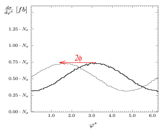
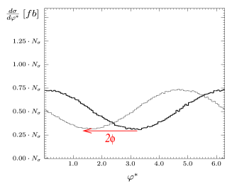
Figure 2: The acoplanarity distribution (angle $\varphi^{*}$) of the $\rho^{+}\rho^{-}$ decay products in the rest frame of the $\rho^{+}\rho^{-}$ pair. Gaussian smearing of $\pi$’s and Higgs boson momenta, are included. Only events where the signs of the energy differences $y_{1}$ and $y_{2}$ are the same, if calculated using the method described in Ref. [19] and if calculated with the help of the $\tau$ impact parameter Ref. [20], are taken. The thick line corresponds to a scalar Higgs boson, the thin line to a mixed one. The left figure contains events with $y_{1}y_{2}>0$, the right one is for $y_{1}y_{2}<0$.

The fitting procedure was repeated 400 times with acoplanarity distributions extracted from independent samples of 1 ab^-1 luminosity each, with a nominal value of $\phi=\pi/4$. A precision on $\phi$ from such a pseudo-experiment of approximately 6^∘ can be anticipated.

4 Summary

The combination of generators for production and decay of intermediate states, require careful treatment of the spin degrees of freedom. In some cases one can restrict spin states to pure helicities; then generation of intermediate states for individual particles can be performed first, and decays of each individual particle can be performed later. The general case, when full quantum mechanical spin correlations are included was also discussed. Technical constraints for the solution based on kinematical information provided by the production programme to be used by the decay routines, were presented. In this context gramatic rules on how event records are filled in were discussed as well.

Finally discussion of observable for the Higgs boson parity measurement at LC, based on such a technical solution was presented in detail, as an example. It was shown, on the basis of careful Monte Carlo simulation of both theoretical and detector effects that with the typical parameters of the future detector and Linear Collider set-up the hypotesis of the admixture of pseudoscalar coupling to the otherwise Standard Model 120 GeV Higgs boson can be measured up to 6^o error on the mixing angle.

5 Acknowledgements

I am grateful to co-authors: G. Bower, C. Biscarat, K. Desch, P. Golonka, A. Imhof, B. Kersevan, T. Pierzchała, E. Richter-Was and M. Worek of the papers and related activities which lead to the presented talk.

References

- [1] ATLAS Collaboration, CERN/LHCC/99-15.
- [2] NLC Collaboration, SLAC-R-571.
- [3] F. . Richard, J. R. Schneider, , D. Trines, and A. Wagner, (eds.) hep-ph/0106314.
- [4] Particle Data Group Collaboration, C. Caso et al., Eur. Phys. J. C3 (1998) 1–794.
- [5] E. Boos et al., hep-ph/0109068.
- [6] S. Jadach, B. F. L. Ward, and Z. Wa̧s, Comput. Phys. Commun. 79 (1994) 503.
- [7] S. Jadach, Z. Wa̧s, R. Decker, and J. Kühn, Comput. Phys. Commun. 76 (1993) 361.
- [8] M. Jeżabek, Z. Wa̧s, S. Jadach, and J. Kühn, Comput. Phys. Commun. 70 (1992) 69.
- [9] S. Jadach, J. H. Kühn, and Z. Wa̧s, Comput. Phys. Commun. 64 (1990) 275.
- [10] S. Jadach and Z. Wa̧s, Comput. Phys. Commun. 36 (1985) 191.
- [11] S. Jadach and Z. Was, Acta Phys. Polon. B15 (1984) 1151.
- [12] T. Pierzchała, E. Richter-Wa̧s, Z. Wa̧s, and M. Worek, Acta Phys. Polon. B32 (2001) 1277, hep-ph/0101311.
- [13] P. Golonka et al., hep-ph/0312240, .
- [14] American Linear Collider Working Group Collaboration, T. Abe et al., page 123 and references therein., hep-ex/0106056.
- [15] M. Kramer, J. H. Kühn, M. L. Stong, and P. M. Zerwas, Z. Phys. C64 (1994) 21, hep-ph/9404280.
- [16] B. Grza̧dkowski and J. F. Gunion, Phys. Lett. B350 (1995) 218, hep-ph/9501339.
- [17] T. Sjostrand et al., Comput. Phys. Commun. 135 (2001) 238, hep-ph/0010017.
- [18] Z. Wa̧s and M. Worek, Acta Phys. Polon. B33 (2002) 1875, hep-ph/0202007.
- [19] G. R. Bower, T. Pierzchała, Z. Wa̧s, and M. Worek, Phys. Lett. B543 (2002) 227, .
- [20] K. Desch, Z. Wa̧s, and M. Worek, Eur. Phys. J. C29 (2003) 491, hep-ph/0302046.