Neutrinos from SN1987A: flavor conversion and interpretation of results

Cecilia Lunardini^a,1 and Alexei Yu. Smirnov^b,c,2

^a Institute for Advanced Study, Einstein drive, 08540 Princeton, New Jersey, USA

^b The Abdus Salam ICTP, Strada Costiera 11, 34100 Trieste, Italy

^c Institute for Nuclear Research, RAS, Moscow 123182, Russia.

After recent results from solar neutrino experiments and KamLAND we can definitely say that neutrinos from SN1987A underwent flavor conversion, and the conversion effects must be taken into account in the analysis of the data. Assuming the normal mass hierarchy of neutrinos we calculate the permutation factors $p$ for the Kamiokande-2, IMB and Baksan detectors. The conversion inside the star leads to $p=0.28-0.32$; the oscillations in the matter of the Earth give partial (and different for different detectors) regeneration of the original $\bar{\nu}_{e}$ signal, reducing this factor down to 0.15 - 0.20 (at $E=40$ MeV). We study in details the influence of conversion on the observed signal depending on the parameters of the original neutrino spectra. For a given set of these parameters, the conversion could lead to an increase of the average energy of the observed events up to 50% and of the number of events by a factor of 2 at Kamiokande-2 and by a factor of 3 - 5 at IMB. Inversely, we find that neglecting the conversion effects can lead up to 50% error in the determination of the average energy of the original $\bar{\nu}_{e}$ spectrum and about 50% error in the original luminosity. Comparing our calculations with experimental data we conclude that the Kamiokande-2 data alone do not favor strong conversion effect, which testifies for small difference of the original $\bar{\nu}_{e}$ and $\bar{\nu}_{\mu}$ spectra. In contrast, the combined analysis of the Kamiokande and IMB results slightly favors strong conversion effects (that is, large difference of the original spectra). In comparison with the no oscillation case, the latter requires lower average energy and higher luminosity of the original $\bar{\nu}_{e}$ flux.

¹ E-mail: lunardi@ias.edu ² E-mail: smirnov@ictp.trieste.it

1 Introduction

After recent results from solar neutrino experiments, and first of all SNO [1, 2, 3], as well as from the reactor experiment KamLAND [4], which have selected the Large Mixing Angle (LMA) MSW solution of the solar neutrino problem, we can definitely say that neutrinos from SN1987A got converted. The neutrino flavor transformations influenced the signals observed in 1987 by Kamiokande-2 (K2)[5, 6], IMB [7, 8] and Baksan [9]. Conversion effects must be taken into account in the analysis of the data and in the determination of the properties of the original neutrino fluxes. Results obtained without conversion are to some extent incorrect.

The conversion of neutrinos associated to SN1987A has been extensively studied before (see [10]-[22] for an incomplete list of references). Here we comment on some papers which are relevant for our present discussion.

It was suggested [23] that the difference of signals detected by the K2 and IMB detectors can be explained partially by the oscillations of neutrinos in the matter of the Earth since the distances crossed by neutrinos on the way to these two detectors were different. The suggestion implied, however, a large lepton mixing, which was not a favored idea at that time. The detailed calculations have been done 13 years later [18], when certain hints appeared that LMA could be the correct solution of the solar neutrino problem.

In connection to SN1987A, Wolfenstein considered antineutrino conversion in the star in the case of large mixing [10]. He concluded that conversion leads to a harder energy spectrum of the observed events and, possibly, to a larger number of events.

In the attempt to restrict the large lepton mixing, the conversion of antineutrinos in the non-resonance channel has been considered in details [16]. From the analysis of the SN1987A data a bound on the permutation factor ($p<0.35$), and consequently,on the mixing angle has been obtained. It was found that the bound is weaker in the LMA range, and the Earth matter effect further relaxes it.

A detailed analysis of the SN1987A data based on the Poisson statistics has been performed by Jegerlehner et al. [17], who found that the data do not allow a definite conclusion on the oscillations hypothesis. In the event that a large neutrino mixing is confirmed (as it has been recently), the data analysis would point toward average neutrino energies (at production in the star) lower than what theoretically predicted. By combining solar and SN1987A data, the authors of refs. [20, 21] concluded that the LMA region was the most suitable, among the large mixing solutions of the solar neutrino problem, to reconcile SN1987A data and predictions from numerical supernova codes, in agreement with [16].

In ref. [18], following the early suggestion [23], we have considered the possibility that certain features of the energy spectra of the events detected by K2 and IMB can be explained by neutrino oscillations in the matter of the Earth. This fixes several bands in the $\Delta m^{2}-\cos 2\theta$ plane. It was concluded that the data favor the parameters of LMA solution and the normal mass hierarchy. The inverted mass hierarchy is disfavored, unless the $1-3$ mixing angle is very small [19] (see however [22]).

The combined analysis of results from solar neutrino experiments and KamLAND lead to the values of oscillation parameters

$$\Delta m^{2}=7.1^{+3.2}_{-2.2}\cdot 10^{-5}{\rm eV}^{2},~{}~{}~{}\tan^{2}\theta=0.40\pm 0.10~{},$$ (1)

which coincides with the third band (from the bottom in $\Delta m^{2}$ scale) found in [18].

In this paper we revisit the conversion of neutrinos from SN1987A using the latest information on neutrino mass spectrum and mixing. We address the questions of how neutrinos were converted, how conversion modified the observed signals and what could be the error in the determination of the original neutrino fluxes if conversion is not taken into account.

The analysis of the SN1987A data and a determination of the original spectra as precise as possible are needed not only to understand what happened in 1987 but also to compare with the results of future detections of neutrino bursts from supernovae. Detections of supernova neutrinos are rare events and furthermore each supernova is unique. Indeed, the mass of the progenitor, luminosity, rotation, magnetic fields, chemical composition can be substantially different, and, as a consequence, the properties of the neutrino fluxes can vary. Thus, future high statistics detections are not expected to reproduce the same features as those of SN1987A, but will give somehow complementary information. The comparison of neutrino signals from different supernovae would be extremely important for understanding the latest stage of star evolution, the dynamics of core collapse and explosion.

The paper is organized as follows. In sec. 2 we consider conversion of antineutrinos and calculate the $\bar{\nu}_{e}$ survival probabilities and permutation factors for Kamiokande-2, IMB and Baksan. In sec. 3 the effects of conversion on the observed signals are studied depending on the parameters of the original spectra. In sec. 4 we compare the predictions with the experimental results and make some indicative conclusions on the properties of the original fluxes. The results are summarized in sec. 5.

2 Neutrino conversion. Permutation factor

As a consequence of the equality of the original $\bar{\nu}_{\mu}$ and $\bar{\nu}_{\tau}$ fluxes, $F_{\bar{\mu}}^{0}=F_{\bar{\tau}}^{0}\equiv F_{\bar{x}}^{0}$, the conversion effects in the antineutrino channel are described by the unique probability $P_{ee}\equiv P(\bar{\nu}_{e}\rightarrow\bar{\nu}_{e})$ which is the total $\bar{\nu}_{e}$ survival probability from the production point to the detector [24] (see however [25]). $P_{ee}$ takes into account the conversion/oscillation effects inside the star, on the way from the star to the Earth and oscillations in the matter of the Earth. Using $P_{ee}$, the electron antineutrino flux at the detector, $F_{\bar{e}}$, can be written in terms of the original fluxes as

$$F_{\bar{e}}=F_{\bar{e}}^{0}+(1-P_{ee})\Delta F^{0},$$ (2)

where

$$\Delta F^{0}\equiv F_{\bar{x}}^{0}-F_{\bar{e}}^{0}$$ (3)

is the difference of original fluxes. The combination

$$p\equiv 1-P_{ee}$$ (4)

is often called the permutation factor (indeed, if $P_{ee}=0$, $p=1$ and $F_{\bar{e}}=F_{\bar{x}}^{0}$, that is, as a result of conversion the initial spectra are permuted).

After the recent determination of the oscillation parameters, and with a few plausible assumptions, the physics of conversion is basically determined and the probability $P_{ee}=P_{ee}(E)$ can be calculated reliably.

In general, taking into account the loss of coherence between mass eigenstates on the way from the star to the Earth, we can write

$$P_{ee}=\sum_{i}P_{ei}^{SN}\times P_{ie}^{Earth},$$ (5)

where $P_{ei}^{SN}$ is the probability of the $\bar{\nu}_{e}\rightarrow\bar{\nu}_{i}$ transition inside the star, and $P_{ie}^{Earth}$ is the probability of $\bar{\nu}_{i}\rightarrow\bar{\nu}_{e}$ transition inside the Earth. Here $\bar{\nu}_{i}$ are the neutrino mass eigenstates.

We assume the following.

• There are only three neutrinos, and if additional (sterile) neutrinos exist, their mixings with active neutrinos are negligible.

• Neutrinos have normal mass hierarchy, or if the hierarchy is inverted, the 1-3 mixing is very small, so that its effect can be neglected (see [24]).

• The density profile in the region of the 1-2 resonance coincides with the progenitor profile during the neutrino burst ($\sim 10$ s). It is not affected by shock wave propagation. Even if the profile changes with time, the adiabaticity character of the conversion remains unchanged due to the large 1-2 mixing.

(We will comment on effects of possible relaxation of these conditions in the sec. 5.)

Under the above assumptions the dynamics of neutrino conversion is completely determined:

1). Inside the star the electron antineutrinos are adiabatically converted into the mass eigenstate $\bar{\nu}_{1}$ [24]

$$\bar{\nu}_{e}\rightarrow\bar{\nu}_{1},$$ (6)

and consequently, $P_{e1}^{SN}=1$, whereas $P_{ei}^{SN}=0$ for $i\neq 1$. Indeed, in the assumption of normal mass hierarchy there are no level crossings in the antineutrino channel. Furthermore, in the production point the mixing is strongly suppressed, so that there we have $\bar{\nu}_{e}=\bar{\nu}_{1m}$, where $\bar{\nu}_{1m}$ is the eigenstate of the neutrino propagation in matter. For the parameters (1) the propagation is highly adiabatic and so the neutrino state coincides with $\bar{\nu}_{1m}$ during the whole propagation. At the surface of the star (zero matter density) $\bar{\nu}_{1m}$ equals $\bar{\nu}_{1}$. Corrections due to possible deviations from the adiabaticity are negligible.

2). Being an eigenstate of the Hamiltonian in vacuum, $\bar{\nu}_{1}$ propagates without any change from the surface of the star to the Earth.

3). Inside the matter of the Earth $\bar{\nu}_{1}$ oscillates, in particular to $\bar{\nu}_{e}$:

$$\bar{\nu}_{1}\rightarrow\bar{\nu}_{e}.$$ (7)

We denote the probability of this transition as $P_{1e}^{Earth}$.

According to this physical picture and eq. (5), the survival probability can be written immediately:

$$P_{ee}=P_{1e}^{Earth}.$$ (8)

Thus, the total survival $\bar{\nu}_{e}\rightarrow\bar{\nu}_{e}$ probability simply coincides with $P_{1e}^{Earth}$ inside the Earth. If the star is not shielded by the Earth, we find

$$P_{1e}^{Earth}=|U_{e1}|^{2}\equiv\cos^{2}\theta_{13}\cos^{2}\theta_{12}$$ (9)

in the standard parameterization of the vacuum mixing matrix (see e.g. [26]). Furthermore, if the 1-3 mixing is small enough the probability equals

$$P_{ee}\approx\cos^{2}\theta_{12}~{},$$ (10)

where the angle $\theta_{12}$ is immediately obtained from the analysis of the solar neutrino data and KamLAND results in the two neutrino framework, eq. (1).

If the 1-3 mixing is near the present upper bound, $\sin^{2}\theta_{13}\mathrel{\vbox{\hbox{$<$}\nointerlineskip\hbox{$\sim$}}}0.06$ [27, 28, 29, 30], and we are interested in $\sim 10\%$ corrections, the complete expression (9) should be used. The solar neutrino data allow us to measure immediately the combination $\cos^{4}\theta_{13}\sin^{2}\theta_{12}$ in high energy experiments and $\cos^{4}\theta_{13}(1-0.5\sin^{2}2\theta_{12})$ in future low energy experiments. These combinations differ from that in eq. (9), therefore independent measurements of $\theta_{13}$ are needed to know $P^{Earth}_{1e}$ accurately. In the present discussion of the SN1987A signal we can neglect corrections due to non-zero 1-3 mixing, since the errors produced in doing so are within the present accuracy of determination of $\theta_{12}$.

The probability of oscillations inside the Earth can be written as

$$P_{1e}^{Earth}\equiv|U_{e1}|^{2}+\bar{f}_{reg},$$ (11)

where $\bar{f}_{reg}$ is called the $\bar{\nu}_{e}$ regeneration factor. Notice that $\bar{f}_{reg}>0$, because inside the Earth the matter density is higher than in the cosmic space. So, there is a partial return to the initial condition of high density in the production point, where the neutrino state is $\bar{\nu}_{e}$. Thus, the oscillations inside the Earth weaken the net conversion effect.

In the two neutrino context, the permutation factor can be written then as

$$p=\sin^{2}\theta_{12}-\bar{f}_{reg},$$ (12)

and the flux of the electron antineutrinos at the detector equals:

$$F_{\bar{e}}=F_{\bar{e}}^{0}+p\Delta F^{0}\approx F_{\bar{e}}^{0}+(\sin^{2}\theta_{12}-\bar{f}_{reg})\Delta F^{0}.$$ (13)

In spite of its simplicity, this expression gives a precise description of the neutrino conversion effect. The permutation factor does not depend on time during the neutrino burst, in the assumption that the matter density profile in the star does not undergo a drastic time evolution.

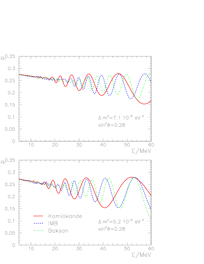
Figure 1: The permutation factor, $p=1-P_{1e}$, as a function of the neutrino energy at Kamiokande-2, IMB and Baksan. The two panels refer to two choices of the oscillation parameters from the LMA allowed region, one of which (upper panel) is the best fit set of values in eq. (1). For illustration purposes, we have averaged $p$ over energy according to eq. (14), with $\Delta E=2$ MeV.

We have performed exact numerical calculations of the probability $P_{1e}^{Earth}$ and the regeneration factor using the Earth density profile from [31]. The fig. 1 shows the permutation factor $p=1-P_{1\bar{e}}^{Earth}$ for Kamiokande-2, IMB and Baksan detectors for two different choices of the oscillation parameters from the LMA allowed region. To remove the unobservable fast oscillations we have averaged the probability over energy as follows:

$$\langle P(E)\rangle=\frac{1}{\Delta E}\int^{E+\Delta E/2}_{E-\Delta E/2}P(E^{\prime})dE^{\prime}~{}.$$ (14)

In the figures $\Delta E=2$ MeV was taken for illustration.
The following remarks are in order.

Due to the larger distance crossed by neutrinos inside the Earth, for the IMB detector the frequency of the oscillatory curve in the energy scale is twice as large as the frequency for K2. The depth of oscillations is nearly the same for all detectors, but the phase of oscillations is different.

Also the averaged permutation factor $\bar{p}$ has the same energy dependence for all detectors: For the best fit values of oscillation parameters (upper panel) it decreases from 0.28 down to 0.25 at $E=25$ MeV and 0.23 at $E=40$ MeV.

For K2, at low energies ($E<25$ MeV), the oscillations in the matter of the Earth are essentially averaged out. For higher energies the averaging is not complete. Notice that the minima of the oscillatory curve are at $E=30$ ($p=0.21$ ) and 40 MeV ($p=0.19$). For IMB the minima are at 36 MeV and 43 MeV ($p=0.19$).

For comparison we show also the permutation factors for $\Delta m^{2}=5.2\cdot 10^{-5}$ eV² which is at the border of the allowed region and in the lower band identified in [18] from the spectral features.

Notice that with the decrease of $\Delta m^{2}$ both the depth of modulation and its period increase. In particular, $f_{reg}\propto 1/\Delta m^{2}$. Now in the minimum of the K2 curve at 40 MeV we find $p=0.15$. The minima are also slightly shifted in energy.

The permutation factor increases with the mixing according to eq. (12); at the same time the regeneration factor changes weakly.

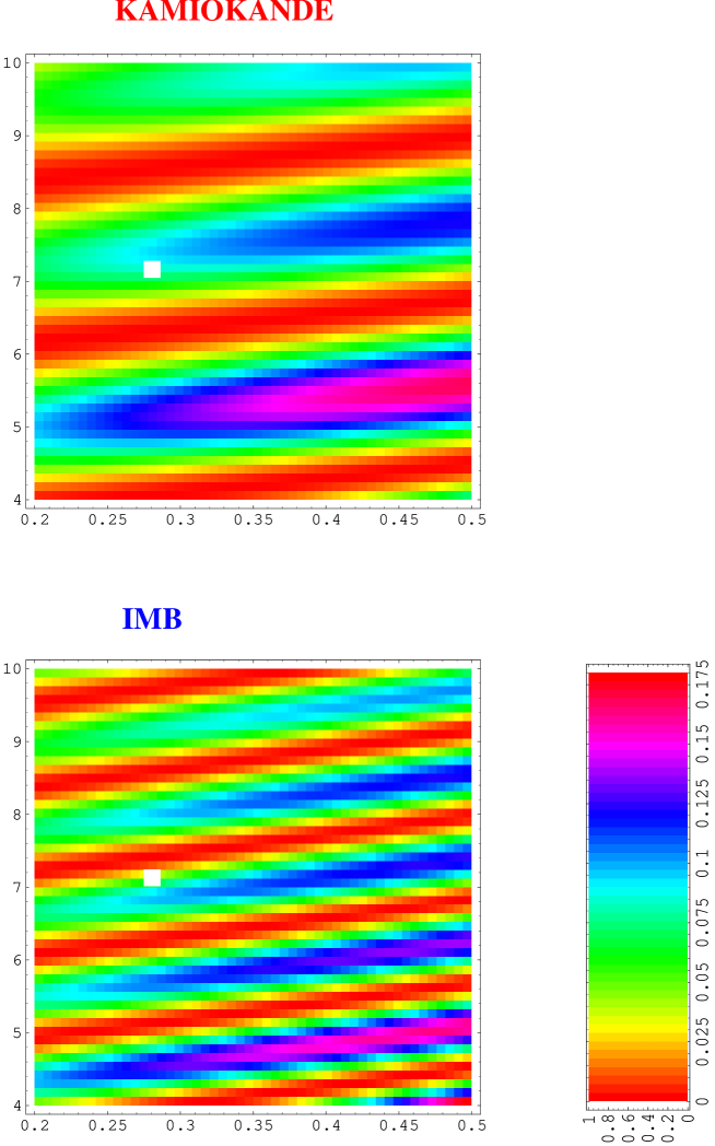
Figure 2: Regions of constant values of the regeneration factor $\bar{f}_{reg}$ at K2 and IMB in the plane $\Delta m^{2}/(10^{-5}~{}{\rm eV^{2}})-\sin^{2}\theta$ (vertical and horizontal axes respectively), for neutrino energy $E=40$ MeV. The white squares denote the LMA best fit point, eq. (1).

The fig. 2 shows values of the regeneration factor $\bar{f}_{reg}$ for K2 and IMB in the $\Delta m^{2}-\sin^{2}\theta_{12}$ plane for $E=40$ MeV. For other energies the result can be obtained from fig. 2 by rescaling of $\Delta m^{2}$: $\bar{f}_{reg}(E,\Delta m^{2})=\bar{f}_{reg}(\Delta m^{2}\times(40{\rm MeV}/E))$. For the best fit values of the oscillation parameters we have $\bar{f}_{reg}\simeq 0.08$ at Kamiokande-2 for E = 40 MeV.

Concluding this part we can definitely say, that

• the permutation factor due to conversion inside the star is about 0.2 - 0.4 with most plausible value 0.28 - 0.30;

• for all detectors this factor is modulated significantly by the Earth matter effect, which suppresses the permutation down to $\sim 0.17$ for E = 40 MeV. The modulation effect due to oscillations inside the Earth increases with energy.

The effect inside the star is determined mainly by the mixing $\sin^{2}\theta_{12}$ and practically does not depend on $\Delta m^{2}$. In contrast, the oscillations inside the Earth are very sensitive to $\Delta m^{2}$ and also depend on mixing. Future operation of the KamLAND experiment will allow us to determine $\Delta m^{2}$ even better, and therefore to have more precise determination of the Earth matter effect. Improvements in the determination of the mixing angle may follow from further operation of SNO.

Notice that in spite of the relatively small values of the permutation factor and even smaller Earth matter effect, the influence of conversion on the neutrino fluxes can be strong. Indeed, if the original $\bar{\nu}_{x}$ flux has substantially larger average energy than the $\bar{\nu}_{e}$ flux, then $F_{\bar{e}}^{0}\ll F_{\bar{x}}^{0}$ in the high energy tail of the spectrum, due to the exponential decrease of the fluxes with the increase of energy. Therefore the observed flux at high energy will be dominated by the converted flux (second term in eq. (2)).

3 Conversion effects and original spectra

According to eq. (2) the effect of conversion on the neutrino spectra, and, consequently, on the spectra of observed events, is proportional to the difference of the original $\mathrel{{\bar{\nu}}_{e}}$ and $\mathrel{{\bar{\nu}}_{x}}$ fluxes. In view of the large uncertainties in these original fluxes (see e.g. the summary in [32]) we will study systematically the conversion effects depending on the values of the parameters of the original spectra.

We will use the following parametrization of the instantaneous original fluxes of neutrinos, which depends explicitly on the integral characteristics [32]:

$$F^{0}_{z}(E)=\frac{L_{z}}{4\pi D^{2}E^{2}_{0z}}\frac{(1+\alpha_{z})^{1+\alpha_{z}}}{\Gamma(1+\alpha_{z})}\left(\frac{E}{E_{0z}}\right)^{\alpha_{z}}\exp\left[-(1+\alpha_{z})E/E_{0z}\right]~{},$$ (15)

where $L_{z}$ is the total (integrated over the neutrino energy) luminosity in the flavor $z$ and $E_{0z}$ is the average energy (as it can be checked by explicit calculation); $D$ is the distance to the star; and $\alpha_{z}$ plays the role of a pinching parameter. It is estimated to be in the interval  [32]

$$\alpha_{z}\sim 2-5~{}.$$ (16)

The width of the spectrum (15) equals

$$\gamma(\alpha_{z})\equiv\left[\frac{\langle E^{2}\rangle}{\langle E\rangle^{2}}-1\right]^{1/2}=\frac{1}{\sqrt{1+\alpha_{z}}}~{}.$$ (17)

The Fermi-Dirac spectrum corresponds to $\alpha_{z}\simeq 2.3$.

The parameters of neutrino fluxes change with time during the neutrino burst: $E_{0z}=E_{0z}(t)$, $L_{z}=L_{z}(t)$, $\alpha_{z}=\alpha_{z}(t)$. In particular, the spectra may have two different time components (see e.g. the review in [33] and references therein): one from the accretion phase, and another one from the cooling phase. During these phases the parameters of the spectra can be substantially different whereas within each phase they change slowly.

The integral characteristics of the original spectra relevant for our discussion are the average energy of the electron antineutrino spectrum, $E_{0e}$; the luminosity in the electron antineutrinos, $L_{e}$; the ratio of the average energies of the muon/tau and electron antineutrino spectra, $r_{E}$, and the ratio of the corresponding luminosities, $r_{L}$:

$$r_{E}\equiv\frac{E_{0x}}{E_{0e}},~{}~{}~{}~{}r_{L}\equiv\frac{L_{x}}{L_{e}}~{};$$ (18)

the pinchings of the $\bar{\nu}_{e}$ and $\bar{\nu}_{x}$ spectra, $\alpha_{e}$ and $\alpha_{x}$.

In the following we consider the signals observed in the Cerenkov detectors K2 and IMB. The features of the predicted neutrino signal at Baksan and the consistency with the observed data are discussed at the end of sec. 4. The differential spectra of the detected positrons from $\mathrel{{\bar{\nu}}_{e}}+p\rightarrow e^{+}+n$ are given by

$$\frac{dN^{i}}{d\epsilon}=N^{i}_{T}\int_{-\infty}^{+\infty}d\epsilon^{\prime}{\cal R}^{i}(\epsilon,\epsilon^{\prime}){\cal E}^{i}(\epsilon^{\prime})\int dEF_{e}^{i}(E)\frac{d\sigma(\epsilon^{\prime},E)}{d\epsilon^{\prime}}~{},$$ (19)

where $i={\rm K2,IMB}$, $\epsilon$ and $\epsilon^{\prime}$ are the observed and the true energies of the positron respectively, $N_{T}^{i}$ is the number of target particles in the fiducial volume, ${\cal E}^{i}$ is the detection efficiency. In (19) the energy resolution function, ${\cal R}^{i}(\epsilon,\epsilon^{\prime})$, is taken in the Gaussian form with $\sigma_{\epsilon}=0.87\sqrt{\epsilon/{\rm MeV}}$ for K2 [6] and $\sigma_{\epsilon}=1.16\sqrt{\epsilon/{\rm MeV}}$ for IMB [7]. The fluxes of antineutrinos at the detectors, $F^{i}_{e}(E)$ are given by eqs. (15) and (13). We use the differential cross section of the detection reaction, ${d\sigma(\epsilon^{\prime},E)/d\epsilon^{\prime}}$, calculated in [34]. The conversion effects ($p^{i}$) have been found using the best fit values of oscillation parameters given in eq. (1).

The signals at the various detectors will be characterized by the following integral characteristics.

- rate, or total number of the observed events $N^{i}$:

$$N^{i}=\int_{\epsilon_{th}^{i}}^{+\infty}d\epsilon\frac{dN^{i}}{d\epsilon};$$ (20)

- the average energy of the detected (electron antineutrino) events, $\bar{\epsilon}^{i}$:

$$\bar{\epsilon}^{i}=\frac{1}{N^{i}}\int_{\epsilon_{th}^{i}}^{+\infty}d\epsilon~{}\epsilon\frac{dN^{i}}{d\epsilon};$$ (21)

- width of the observed spectrum:

$$\Gamma^{i}=\left[\frac{\langle\epsilon^{2}\rangle^{i}}{(\bar{\epsilon}^{i})^{2}}-1\right]^{1/2},$$ (22)

where

$$\langle\epsilon^{2}\rangle^{i}=\frac{1}{N^{i}}\int_{\epsilon_{th}^{i}}^{+\infty}d\epsilon~{}\epsilon^{2}\frac{dN^{i}}{d\epsilon}.$$ (23)

We calculate these characteristics of the K2 and IMB signals as functions of the parameters of the original neutrino spectra. The results can be considered as instantaneous characteristics of observed events or as the integral characteristics if the parameters of the original spectra do not change during the neutrino burst. This matches the constant temperature model presented in the upper panel of Table 4 in ref. [33] .

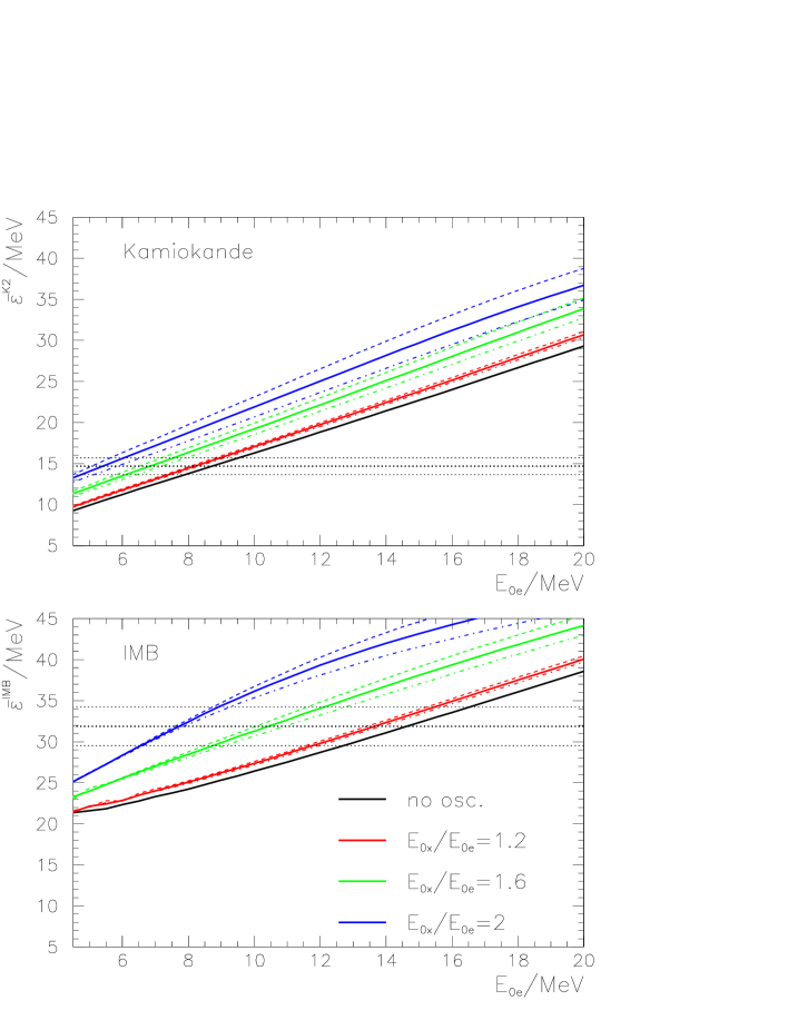
Figure 3: The average energy of positrons in the detectors K2 and IMB, $\bar{\epsilon}^{i}$, as a function of the average energy of the original $\bar{\nu}_{e}$ flux, $E_{0e}$, for the best fit LMA parameters (eq. (1), see also fig. 1) and different values of $r_{E}=E_{0x}/E_{0e}$ (see legend) and $r_{L}=L_{x}/L_{e}$. The solid, dashed and dotted-dashed lines correspond to $r_{L}=1,1.5,0.667$ respectively. The no oscillation case (or, equivalently, the case $r_{E}=1$) is shown for comparison. The dotted (horizontal) lines represent the values of $\bar{\epsilon}^{i}$ extracted from the data for each experiment, with the $1\sigma$ error (eq. (31)).

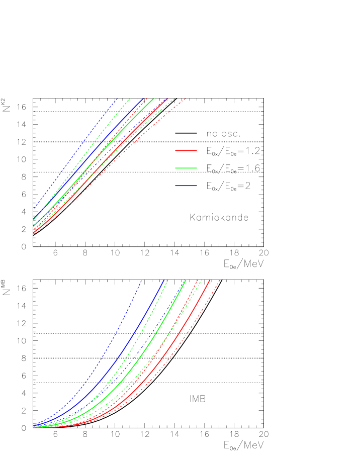
Figure 4: The predicted numbers of events at K2 and IMB as a function of the average energy of the original $\bar{\nu}_{e}$ flux, $E_{0e}$. The line identification, as well as the oscillation parameters, are the same as in fig. 3. The dotted (horizontal) lines represent the experimental result with the $1\sigma$ error (eq. (26)). We use $L_{e}=L_{0}=5.3\cdot 10^{53}$ ergs.

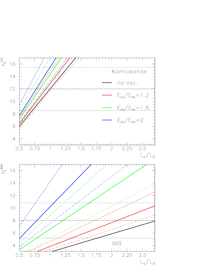
Figure 5: The predicted numbers of events at K2 and IMB as a function of the ratio $L_{e}/L_{0}$ ($L_{0}=5.3\cdot 10^{52}$ ergs) for $E_{0e}=11$ MeV. The line identification, as well as the oscillation parameters, are the same as in fig. 3. The dotted (horizontal) lines represent the experimental result with the $1\sigma$ error (eq. (26)).

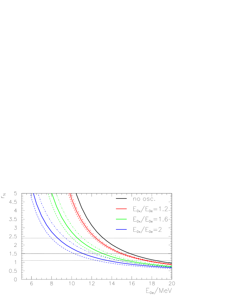
Figure 6: The ratio of the numbers of events at K2 and IMB, $r_{N}$, as a a function of the average energy of the original $\bar{\nu}_{e}$ flux, $E_{0e}$. The line identification, as well as the oscillation parameters, are the same as in fig. 3. The dotted (horizontal) lines represent the experimental result with the $1\sigma$ error (eq. (40)).

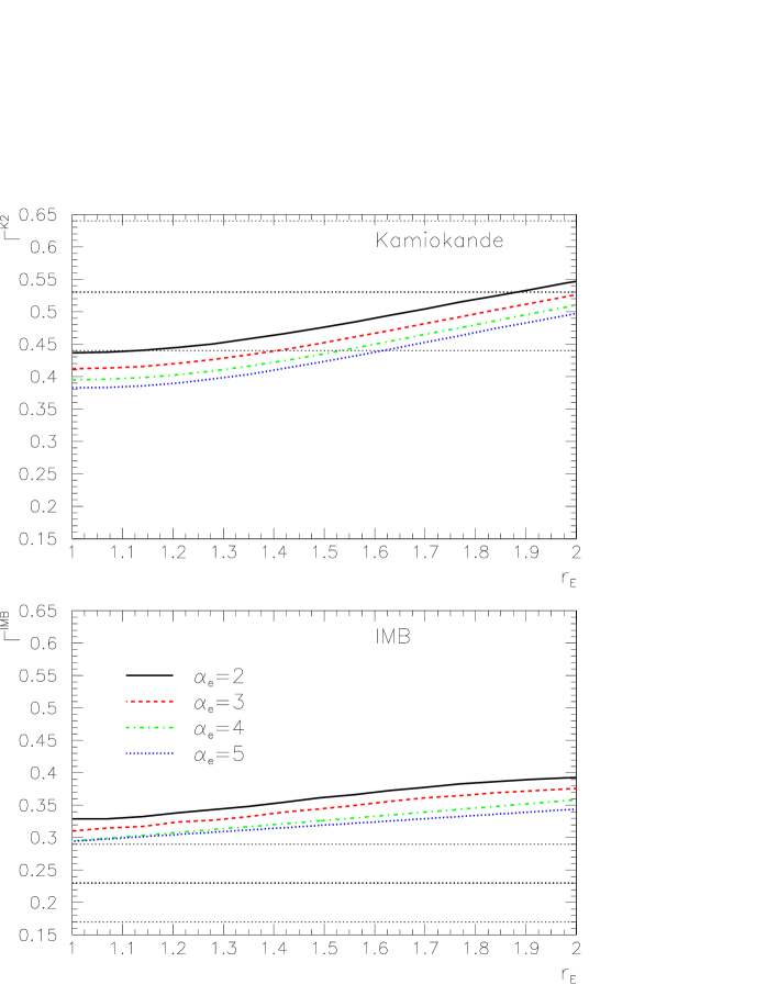
Figure 7: The predicted widths of the K2 and IMB energy spectra as a function of $r_{E}$ for different values of the pinching parameter $\alpha_{e}$. The oscillation parameters are the same as in fig. 3. We have taken $E_{0e}=11$ MeV, $r_{L}=1$ and $\alpha_{x}=\alpha_{e}$. The dotted (horizontal) lines represent the experimental result with the $1\sigma$ error, eq. (32).

Results for the observed numbers of events and average energies are presented in the figs. 3-6, and summarized in the Table 1. They refer to the case in which $\alpha_{e}=\alpha_{x}=3$, so that the corresponding widths are equal and fixed to the value $\gamma=0.5$, according to eq. (17). Fig. 7 shows results for the widths $\Gamma^{i}$ and illustrates their dependence on $\alpha=\alpha_{e}=\alpha_{x}$. A further illustration of the $\alpha$-dependence is given in Table 2.

	no oscill.	$r_{E}=1.2$	$r_{E}=1.6$	$r_{E}=2$
$\bar{\epsilon}^{K2}/\bar{\epsilon}_{no~{}osc.}^{K2}-1$	0	0.04-0.06	0.18	0.35
$\bar{\epsilon}^{IMB}/\bar{\epsilon}_{no~{}osc.}^{IMB}-1$	0	0.04	0.18	0.35-0.37
$N^{K2}/N_{no~{}osc.}^{K2}-1$	0	0.08	0.19	0.29
$N^{IMB}/N_{no~{}osc.}^{IMB}-1$	0	0.27	0.36	1.64
$E_{0e}/MeV$ (from $\bar{\epsilon}^{K2}$)	8.8	8.2	6.7	5.4
$E_{0e}/MeV$ (from $\bar{\epsilon}^{IMB}$)	14.7	13.7	10.4	7.6
$L_{e}/L_{0}$ ($N^{K2}=12$)	1	0.93	0.78	0.76
$L_{e}/L_{0}$ ($N^{IMB}=8$)	2.75	2.17	1.2	0.76
$\bar{\epsilon}^{K2}/\bar{\epsilon}^{IMB}$	0.65	0.64	0.63	0.62
$N^{K2}/N^{IMB}$	4.2	3.5	2.2	1.5

Table 1: Effect of the neutrino conversion on characteristics of observable K2 and IMB signals and extracted parameters of the original neutrino spectra. The numbers of events and luminosities correspond to $E_{0e}=11$ MeV and $r_{L}=1$.

Let us summarize the effects of flavor conversion:

1). The conversion leads to an increase of the average energy of the observed events (fig. 3). According to fig. 3, for K2 the dependence of $\bar{\epsilon}^{i}$ on $E_{0e}$ is linear in a wide interval of energies ($E_{0e}>5$ MeV) due to the low energy threshold, and it can be approximated with good accuracy by

$$\bar{\epsilon}\approx A(r_{E},r_{L})E_{0e}+B(r_{E},r_{L}).$$ (24)

We find $A(r_{E},1)=1.24,~{}1.32,~{}1.47,~{}1.58$ for $r_{E}=1.0,~{}1.2,~{}1.6,~{}2.0$ respectively. For IMB, due to the higher energy threshold, the the dependence is linear in a restricted interval only.

Due to their dependence on the difference of the original $\mathrel{{\bar{\nu}}_{e}}$ and $\mathrel{{\bar{\nu}}_{x}}$ fluxes, eq. (2), the conversion effects increase with $r_{E}$. In the wide energy range $E_{0e}=(8-11)$ MeV (and for $r_{L}=1$), both $\bar{\epsilon}^{K2}$ and $\bar{\epsilon}^{IMB}$ increase by up to $\sim 37\%$ with the variation of $r_{E}$ between 1 and 2. This change is substantially larger than the $1\sigma$ experimental interval, which equals $\sim 7.2-7.5\%$. As shown in fig. 3, for $E_{0e}=11$ MeV the values of the average energies are in the intervals $\bar{\epsilon}^{K2}=17.5-23.5$ and $\bar{\epsilon}^{IMB}=27.5-37.7$.

The dependence of $\bar{\epsilon}^{i}$ on $r_{L}$ is mild at low-intermediate energies and becomes slightly stronger at high $E_{0e}$ and for larger $r_{E}$. For $r_{E}=1.6$ we have that as $r_{L}$ varies from 0.67 to 1.5 the change in $\bar{\epsilon}^{i}$ does not exceed $\sim 7\%$ for K2 and $\sim 3.5\%$ for IMB. The latter dependence is weaker due to the higher IMB energy threshold, which results in a reduced sensitivity of the IMB signal to the softer component of the spectrum due to the original $\mathrel{{\bar{\nu}}_{e}}$ flux.

The plot (fig. 3) allows us to estimate the errors in the determination of $E_{0e}$ in the case when conversion is not taken into account. One can see that in the no-oscillation case the observed average energy at K2 corresponds to $E_{0e}=8.8$ MeV, while the IMB observation is reproduced for $E_{0e}=14.7$ MeV. With conversion these two values become as low as $E_{0e}=5.4$ MeV and $E_{0e}=7.6$ MeV respectively.

So, not taking into account conversion can lead to an error in the determination of the average energy (or temperature) of the original spectrum as large as 40 - 50%.

2). The conversion leads in general to an increase of the number of events (an exception is the case of low non-electron flux, $r_{L}<1$, and $r_{E}\sim 1$). The number of events is proportional to the $\bar{\nu}_{e}$ luminosity, $L_{e}$:

$$N^{i}=N_{0}^{i}(E_{0e},r_{L},r_{E})\frac{L_{e}}{L_{0}},$$ (25)

where $N_{0}^{i}$ is the number of events in the detector $i$ for a fixed luminosity $L_{0}$. For definiteness we take $L_{0}=5.3\cdot 10^{53}$ ergs, which is the integral luminosity in the $\mathrel{{\bar{\nu}}_{e}}$ species determined in ref. [33] from the analysis of data in the constant temperature scenario without oscillations.

In fig. 4 we show the dependences of $N_{0}^{i}$ for K2 and IMB on $E_{0e}$ for different values of the ratios $r_{L}$ and $r_{E}$. Also shown are the lines which correspond to the numbers of events observed in these detectors together with the $1\sigma$ bands.

While $N_{0}^{K2}$ increases nearly linearly with $E_{0e}$ (for $E_{0e}>6$ MeV), the dependence of $N_{0}^{IMB}$ is stronger as an effect of the higher energy threshold and slow rise of the detection efficiency with energy.

For $E_{0e}=11$ MeV and $r_{L}=1$ the increase of $N_{0}^{i}$ with $r_{E}$ does not exceed $\sim 30\%$ for K2, while it can reach a factor of 3.5 at IMB (see Table 2). The increase is more sizable for lower $E_{0e}$, as can be seen in fig. 4.

The numbers of events increase with $r_{L}$: we see a change by $\sim 30\%$ at K2 and by $\sim 75\%$ at IMB for $E_{0e}=11$ MeV and $r_{E}=1.6$.

In fig. 5 we show the dependences of the total numbers of events, $N^{i}$, on $L_{e}$ for $E_{0e}=11$ MeV and different values of the ratios $r_{L}$ and $r_{E}$. This plot allows us to evaluate the error in the determination of the original luminosity if the oscillation effect is not taken into account. The detected number of events $N^{K2}=12$ at K2 can be reproduced without oscillations for $L_{e}=L_{0}=5.3\cdot 10^{52}$ ergs. With the increase of the conversion effect (increase of $r_{E}$ or/and $r_{L}$) the required luminosity decreases (see Table 1). E.g. we find: $L_{e}/L_{0}=0.78$ for $r_{E}=1.6$. For IMB the effect is much stronger: The observed $N^{IMB}=8$ events can be obtained for $L_{e}/L_{0}=2.75$ with no oscillations. The required luminosity decreases down to $L_{e}/L_{0}=1.2$ for $r_{E}=1.6$.

3). The conversion effects for K2 and IMB differ due to

- different Earth matter effect; and

- different experimental characteristics: thresholds and efficiencies of detection.

In fig. 6 we show the ratio of the numbers of events at K2 and IMB, $r_{N}=N^{K2}/N^{IMB}$, as a function of $E_{0e}$. The experimental value is $r_{N}=1.5$. The ratio increases with the decrease of $E_{0e}$. The conversion leads to a decrease of $r_{N}$, thus allowing to reconcile the required energy $E_{0e}$ and the correct value of $N^{K2}/N^{IMB}$. Taking $E_{0e}=11$ MeV and $r_{E}=1$ we find that $r_{N}$ varies between 4.2 and 1.5 depending on $r_{E}$ (Table 1).

In contrast to the numbers of events, the energies of the observed events at K2 and IMB are modified by the conversion in rather similar ways, so that their ratio is not affected significantly: $\bar{\epsilon}^{K2}/\bar{\epsilon}^{IMB}=0.62-0.66$ (see Table 1 and fig. 4). The change is even weaker for lower $E_{0e}$.

The difference of conversion effects can be used to improve the agreement of the IMB and K2 signals (sec. 4).

4). In fig. 7 we show the dependence of the widths of the observed positron spectra, $\Gamma^{i}$, on $r_{E}$ for different values of the pinching parameter $\alpha=\alpha_{e}=\alpha_{x}$ and $r_{L}=1$ (results for other values of $r_{L}$ are almost identical). It appears that this dependence is approximately linear for $r_{E}\mathrel{\vbox{\hbox{$>$}\nointerlineskip\hbox{$\sim$}}}1.2$. Conversion (i.e. $r_{E}>1$) leads to widening of the K2 and IMB observed spectra, and the widening is larger for larger $r_{E}$, reaching $\sim 25-30\%$ for $r_{E}=2$. We see a $\sim 10\%$ decrease of $\Gamma^{K2}$ and $\Gamma^{IMB}$ as $\alpha_{e}$ increases from 2 to 5 (i.e., as the original spectra become more pinched).

scenario $\backslash$ $\alpha$	2	3	4	5
no-oscillation ($\chi^{2}$)	24.05	16.8	17.0	19.2
$N^{K2}$	13.0	11.9	11.2	10.7
$\bar{\epsilon}^{K2}/MeV$	19.4	17.5	16.4	15.5
$\Gamma^{K2}$	0.44	0.41	0.40	0.38
$N^{IMB}$	4.81	2.85	1.84	1.25
$\bar{\epsilon}^{IMB}/MeV$	30.1	27.5	25.9	24.8
$\Gamma^{IMB}$	0.33	0.31	0.30	0.29
“concordance” ($\chi^{2}$)	15.0	11.0	12.4	14.7
$N^{K2}$	14.6	13.0	12.0	11.3
$\bar{\epsilon}^{K2}/MeV$	17.9	16.3	15.3	14.6
$\Gamma^{K2}$	0.47	0.45	0.44	0.43
$N^{IMB}$	4.28	2.59	1.74	1.25
$\bar{\epsilon}^{IMB}/MeV$	30.7	28.5	27.0	26.0
$\Gamma^{IMB}$	0.34	0.32	0.31	0.30

Table 2: Effects of different values of $\alpha=\alpha_{e}=\alpha_{x}$ on the observables in the no-oscillation case with parameters from Loredo & Lamb [33] (lines 1 - 7) and in the case of oscillations with parameters from our concordance scenario given in secs. 3 and 4 (lines 8 - 14).

The dependence of the observables on $\alpha$ is summarized in the Table 2. We show results for two scenarios: (1) the no-oscillation best fit scenario of ref. [33], with $E_{0e}=11$ MeV, $L_{e}=5.3\cdot 10^{52}$  ergs and (2) the “concordance” scenario (see sec. 4) with conversion, $E_{0e}=8$ MeV, $L_{e}=8\cdot 10^{52}$  ergs, $r_{E}=1.6$ and $r_{L}=1$.

With the variation of $\alpha$, all the quantities in the table change by at most $10\%$, with the exception of the number of IMB events, which can vary even by a factor of 2 with respect to the case $\alpha=3$. In particular, the decrease of $\alpha$ down to $\alpha=2$, leads to an increase of $N^{IMB}$ by 65 - 70 %. That is, in the “concordance” scenario a smaller $\alpha$, $\alpha\simeq 2$, could fit the numbers of events better. This however is compensated by the worsening of the fit to the average energies, so that the global fit does not improve.

4 SN1987A data and neutrino fluxes

Using the results of the previous sections we now compare the data with predictions and make qualitative statements on the interpretation of experimental results and the determination of the original neutrino fluxes.

Let us consider the integral characteristics of the signals. We assume that all events are due to $\bar{\nu}_{e}$ interactions and background. After background subtraction (according to [6, 7]), we take the total numbers of events detected by K2 and IMB as

$$N^{K2}=12.0\pm 3.5,~{}~{}~{}~{}N^{IMB}=8.0\pm 2.8.$$ (26)

The experimental value of the average energy of the detected events equals

$$\bar{\epsilon}^{k}=\frac{1}{N^{k}}\sum_{i}\epsilon_{i}^{k}~{},$$ (27)

where the summation runs over all observed events in a given detector. We define the error of the average energy as

$$\Delta\bar{\epsilon}^{k}=\frac{1}{N^{k}}\sqrt{\sum_{i}(\Delta\epsilon^{k}_{i})^{2}},$$ (28)

where $\Delta\epsilon^{k}_{i}$ is the error in the energy determination of the individual event.

Similarly, we calculate the width:

$$\Gamma^{k}=\sqrt{N^{k}\frac{\sum_{i}(\epsilon^{k}_{i})^{2}}{(\sum_{i}\epsilon^{k}_{i})^{2}}-1}~{},$$ (29)

and the associated error:

$$\Delta\Gamma^{k}=\sqrt{\sum_{i}\left(\frac{\partial\Gamma^{k}}{\partial\epsilon^{k}_{i}}\Delta\epsilon^{k}_{i}\right)^{2}}~{}.$$ (30)

From the data we get the average energies:

$$\bar{\epsilon}^{K2}=14.7\pm 1.1~{}{\rm MeV}~{}~{}~{}~{}~{}~{}\bar{\epsilon}^{IMB}=31.9\pm 2.3~{}{\rm MeV},$$ (31)

and the widths:

$$\Gamma^{K2}=0.53\pm 0.1,~{}~{}~{}~{}~{}~{}\Gamma^{IMB}=0.23\pm 0.06~{}.$$ (32)

We show these central values and the $1\sigma$ bands in the figs. 3 - 7.

To compare those results with observations (26, 31) one needs to perform an integration over time, taking into account the time dependence of the parameters of the original spectra (alternatively, one could analyze the data in short periods of time, however the statistics is too small). Indeed, it is expected that during the neutrino burst there is a significant change in the parameters of spectra with time (see e.g. [35] and references therein). However, due to the nearly linear dependences of the observables on the parameters, the relative conversion effect changes with time very weakly.

Let us perform time averaging of the relation (24). If the ratios $r_{E}$ and $r_{L}$ depend on time weakly – which is expected during the cooling phase – then the $A$ and $B$ coefficients are nearly constant and for the time averaged energy we can write

$$\langle\bar{\epsilon}\rangle\approx A(\bar{r}_{E},\bar{r}_{L})\langle E_{0e}\rangle+B(\bar{r}_{E},\bar{r}_{L}),$$ (33)

where $\langle E_{0e}\rangle=\int dtE_{0e}/\Delta t$. This means that the relation (24), and the dependences in fig. 4 can be considered as the relation and dependences between the time averaged characteristics.

Let us now consider numbers of events. Assuming linear dependence of $N_{0}^{i}$ on $E_{0e}$, $N_{0}^{i}\approx C^{i}(r_{E},r_{L})E_{0e}+G^{i}(r_{E},r_{L})$ (which may not be a good approximation for IMB), and weak change or $r_{E}$ and $r_{L}$ with time, we can write:

$$N^{tot,i}=\left[C^{i}(\bar{r}_{E},\bar{r}_{L})\langle{E}_{0e}\rangle_{L}+G^{i}(\bar{r}_{E},\bar{r}_{L})\right]\frac{1}{L_{0}}\int dtL(t),$$ (34)

where

$$\langle{E}_{0e}\rangle_{L}=\frac{\int E_{0e}Ldt}{\int Ldt}.$$ (35)

From this it follows that we can use the relations and figures constructed for instantaneous spectra or – equivalently – the time-independent scenario, also for the case of time-dependence, keeping in mind that the parameters $E_{0e}$, $L_{e}$, $r_{E}$, $r_{L}$ should be considered as some effective parameters obtained by appropriate averaging over the time of the burst. This still can be used to study the compatibility of signals in different detectors, but the real meaning of the parameters extracted is ambiguous and it depends on the detailed time dependence of instantaneous characteristics. In what follows we will use the same notations as in sec. 3, though one should keep in mind that these are effective parameters.

1). Analysis of the Kamiokande-2 data only. In the absence of oscillations, from fig. 3 we extract the value of the (effective) $\bar{\nu}_{e}$ average energy:

$$E_{0e}=8.7\pm 0.9~{}{\rm MeV},~{}~{}~{}(1\sigma).$$ (36)

According to fig. 4, for this energy and $L_{e}=L_{0}$ the number of predicted events equals $N_{e}=7.8\pm 1.5$ which is about $1\sigma$ below of observed number, eq. (26). The exact number of observed events can be reproduced if $L_{e}=1.54L_{0}=8.2\cdot 10^{52}$ ergs.

The conversion leads to a decrease of $E_{0e}$. For instance, for $r_{E}=1.6$ and $r_{L}=1$ we find from fig. 3:

$$E_{0e}=6.8\pm 0.8~{}{\rm MeV},~{}~{}~{}(1\sigma).$$ (37)

According to fig. 4, this gives $N^{K2}=6.3\pm 1.5$ for $L_{e}=L_{0}$. So, correspondingly, a fit to the observed number of events implies even higher integral luminosity: $L_{e}=1.9L_{0}=(10.1\pm 2.4)\cdot 10^{52}$ ergs, which seems rather high, also keeping in mind the low average energies of neutrinos.

So, the K2 data alone disfavor strong conversion effect; though within $2\sigma$ even a strong effect ($r_{E}=1.6$ ) can be easily accommodated.

2). Kamiokande-2 and IMB. For IMB, in the absence of oscillations, we find, from fig. 3:

$$E_{0e}=14.7\pm 1.9~{}{\rm MeV},~{}~{}~{}(1\sigma)$$ (38)

which is more than $3\sigma$ above the K2 result, eq. (36). According to fig. 4 for this energy and $L_{e}=L_{0}$ the number of predicted events equals $N^{IMB}=10+6/-4$ which is in a very good agreement with the experimental result. The precise number of the IMB events can be reproduced for $L_{e}=0.8L_{0}$.

Thus, the IMB signal implies about 2 times higher energies of events and 2 times smaller integral luminosity in comparison with K2.

Conversion leads to a decrease of the extracted energy and luminosity. For $r_{E}=1.6$ and $r_{L}$ we get

$$E_{0e}^{IMB}=10.3\pm 1.7~{}{\rm MeV},~{}~{}~{}(1\sigma).$$ (39)

which is only $2\sigma$ above the K2 result for the same $r_{E}$.

With conversion effects, the agreement of the IMB and K2 results can improve. We can find a “concordance” set of parameters of the original fluxes which give a better description of all the available data: average energies, luminosities and widths. The latter can be affected significantly by the oscillations in the matter of the Earth.

The ratio of the average energies extracted from the K2 and IMB data approaches 1 with the increase of $r_{E}$: $E_{0e}^{IMB}/E_{0e}^{K2}=1.7,1.51,1.43$ for $r_{E}=1.0,1.6,2.0$. Notice however, that the difference does change significantly for $r_{E}>1.6$ being about $2\sigma$. Furthermore, with the increase of $r_{E}$ both the extracted energies $E^{K2}_{0e}$ and $E_{0e}^{IMB}$ decrease, and this makes it difficult to reproduce the total numbers of events, especially for IMB. Considering this, we find that the optimal energy is in the interval $E_{0e}=(7-9)$ MeV, where one can get $1\sigma$ deviation from both K2 and IMB extracted values. This result does not depend on the luminosity $L_{e}$.

Considering the numbers of events, notice that once the correct ratio $r_{N}\equiv N^{K2}/N^{IMB}$ is reproduced, the numbers of events can be obtained by fitting $L_{e}$. From the data we find

$$r_{N}\equiv\frac{N^{K2}}{N^{IMB}}=1.5^{+0.9}_{-0.4}.$$ (40)

However, according to fig. 6, for the small $E_{0e}$ required by the fit of the average energies the ratio $r_{N}$ turns out to be too large. Indeed, for $r_{E}=1$ (i.e., no oscillations), the “optimal” energy is $E_{0e}=10.3$ MeV; for these parameters the ratio of number of events equals $r_{N}=5.3$. We find $E_{0e}\sim 9.6$ MeV and $r_{N}=5.2$ for $r_{E}=1.2$; $E_{0e}\sim 7.7$ MeV and $r_{N}=5.2$ for $r_{E}=1.6$; $E_{0e}\sim 6.2$ MeV and $r_{N}=4.9$ for $r_{E}=2.0$. So, $r_{N}$ is substantially larger than the experimental result and does not change practically by conversion once the parameters are optimized by the average observed energies.

Let us now discuss the widths of the observed spectra $\Gamma^{i}$, shown in fig. 7 (for $E_{0e}=11$ MeV and $r_{L}=1$). One can see (see also eq. (32)), that the IMB spectrum has smaller width than the one of K2. The former is better reproduced without oscillations (or small $r_{E}$) and with large $\alpha$, $\alpha\simeq 5$, while the latter points toward the case of oscillations with $r_{E}\mathrel{\vbox{\hbox{$>$}\nointerlineskip\hbox{$\sim$}}}1.6$ and $\alpha\sim 2$. The widths $\Gamma^{i}$ decrease slightly (by $\sim 10\%$) with the decrease of $E_{0e}$; we refer to Table 2 for results at $E_{0e}=8$ MeV (concordance scenario).

To get an idea about the preferable values of parameters of the original spectra we calculate $\chi^{2}$ defined as

$$\chi^{2}\equiv\sum_{j}\left(\frac{X_{j}-\bar{X}_{j}}{\Delta X_{j}}\right)^{2}$$ (41)

for various sets of the parameters. Here $X_{j}\equiv N^{K2},N^{IMB},\bar{\epsilon}^{K2},\bar{\epsilon}^{IMB},\Gamma^{K2},\Gamma^{IMB}$, are the numbers of events, average energies and widths of the positron spectra observed at Kamiokande2 and IMB.

Without oscillations and $E_{0e}=11$ MeV, $L=L_{0}$, $\alpha_{e}=\alpha_{x}=3$ we find $\chi^{2}=16.2$. With oscillations for $E_{0e}=8$ MeV, $L=8\cdot 10^{52}$ ergs, $\alpha_{e}=\alpha_{x}=3$, $r_{E}=1.6$, $r_{L}=1$, we obtain $\chi^{2}=11.0$ (see Table 2 for the dependence of results on the pinching parameters $\alpha_{z}$). We checked that the improvement in the $\chi^{2}$ is mainly due to the smaller deviation of the predicted $\bar{\epsilon}^{K2}$ from the observed value. This deviation amounts to about 2.6 $\sigma$ for no-oscillations, and to $\sim 1.4~{}~{}\sigma$ for the case with oscillations. Correspondingly, the contribution of $\bar{\epsilon}^{K2}$ to the $\chi^{2}$ decreases from 7 to 2 when oscillations are included. Notice however that with the decrease of $E_{0e}$ implied by conversion effects, substantially larger integral luminosity is required to reproduce the numbers of events. The combination of smaller average energy and larger luminosity corresponds to a larger radius of the neutrinosphere: $R_{ns}\propto E_{0e}^{-2}L^{1/2}$. It follows that in our concordance scenario $R_{ns}$ is about 2.4 times larger than in the no-oscillation scenario, which gives $R_{ns}\simeq 20-30$ Km [33]. This increase is within the range allowed by the several uncertainties of astrophysical nature and by individual variations from one star to another.

Thus we conclude that conversion leads to a certain improvement of the global fit of the data. The improvement requires lower average energies of the original $\bar{\nu}_{e}$ spectrum and higher $\bar{\nu}_{e}$ integral luminosity. Conversion effects lead to a better agreement of the observed average energies with the data sample, but this improvement is compensated partially by a worsening in reproducing the numbers of events.

3). Baksan results. If all the 5 events recorded by Baksan are attributed to signal, analyses of these data without oscillations lead to neutrino luminosities which are much larger than those implied by the K2 and IMB data samples (see the account in ref. [33]). This indicates that part of the Baksan events are due to background, and, in absence of a specific prescription for background subtraction, it is difficult to include the Baksan results in our analysis. In ref. [33] a method to account for a background origin of part of the Baksan events is proposed. Notice that in presence of oscillations the K2 and IMB data require larger neutrino luminosities, therefore it is possible that including neutrino conversion will reduce the number of the Baksan events attributed to background.

4). Spectrum of events. As we have marked in the introduction, the oscillation parameters we use are in the band determined previously from the fit of the energy spectra of K2 and IMB [18] (see also fig. 2). So the oscillation parameters, and in particular $\Delta m^{2}$, are already optimized to get the best description of the spectra of events. We mark that, in contrast with what discussed in [18], here the numbers of events, widths and average energies of the observed positrons depend very weakly (about $\sim 2-5\%$ at most) on the phase of oscillations in the Earth. This is motivated by the larger value of $\Delta m^{2}$ used here, for which the permutation factor has faster oscillations with smaller depth. These oscillations can be seen in figure 2 (in which no averaging has been applied), however in the observed signal they are almost completely averaged out as an effect of the experimental energy resolution.

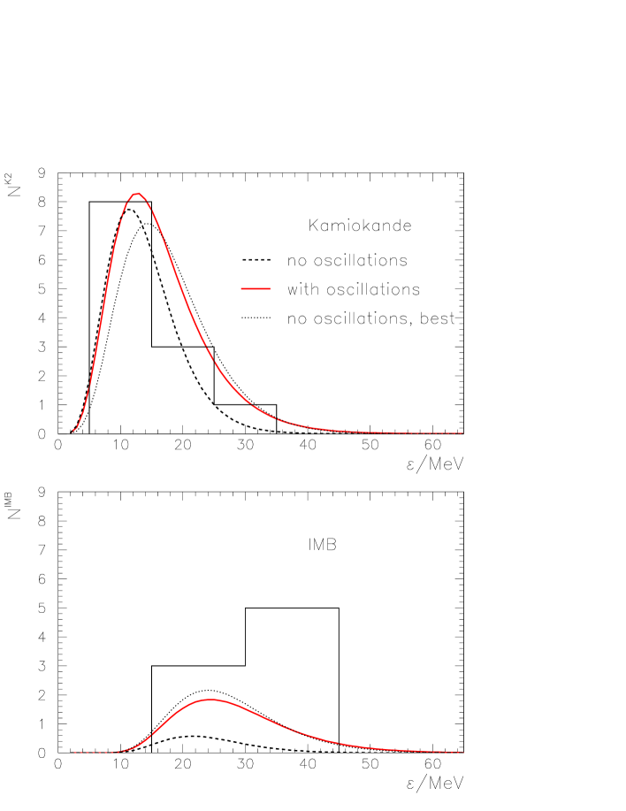
Figure 8: The predicted positron energy spectra at K2 and IMB with and without oscillations. The solid lines correspond to $E_{0e}=8$ MeV, $L_{e}=8\cdot 10^{52}$ ergs, $r_{E}=1.6$, $r_{L}=1$ and the best-fit LMA parameters (eq. (1), see also fig. 1). The dashed lines correspond to the no-oscillation case with the same parameters: $E_{0e}=8$ MeV, and $L_{e}=8\cdot 10^{52}$ ergs. The dotted lines correspond to no-oscillations with the best fit parameters of ref. [33]: $E_{0e}=11$ MeV, $L_{e}=5.3\cdot 10^{52}$ ergs. The histograms show the experimental results.

In fig. 8 we show the calculated spectra of the events at Kamiokande-2 and IMB for the “concordance” set of parameters of the original fluxes: $E_{0e}=8$ MeV, $L_{e}=8\cdot 10^{52}$ ergs, $r_{E}=1.6$, $r_{L}=1$ (solid lines). Also shown are the spectra without oscillation for the best fit parameter set determined in [33] (“constant temperature model”) (dotted) and the spectrum for the concordance set of spectral parameters without oscillations (dashed). Comparing solid and dashed lines we conclude that the conversion effect is significant in the whole energy range for IMB and for $\epsilon>15$ MeV at K2.

At the same time the spectra with best fit values of parameters (without conversion) and with the concordance set of parameters and conversion are rather close. The difference is mainly in the low energy K2 spectrum. We stress that, though similar,the spectra with and without conversion require substantially different parameters of the original spectra.

5 Discussion and Conclusions

1). After the identification of the solution of the solar neutrino problem and KamLAND results, we can definitely say that neutrinos from SN1987A underwent flavor conversion inside the star and oscillations in the matter of the Earth.

In the assumption of the normal mass hierarchy, the conversion probabilities can be calculated with good precision. We find that the permutation factor is about $p=0.28-0.32$ due to conversion inside the star and oscillations in the matter of the Earth suppress the permutation. The Earth effect increases with energy, and at $E\sim 40$ MeV $p$ decreases down to 0.15- 0.20.

2). The conversion effects on observables depend strongly on the properties of the original neutrino fluxes, in particular, on the average energies and widths of the original spectra of $\bar{\nu}_{e}$ and $\bar{\nu}_{\mu/\tau}$. For a given set of these parameters, conversion leads to an increase of the number and of the average energy of the observed events as well as of the widths of the observed spectra. The conversion effects are different for K2 and IMB. By varying parameters in the ranges allowed by astrophysics, we have found that the average energy of events can increase by 30 - 50 % and the number of events by 50 % for K2 and by up to a factor of 3 for IMB.

Vice versa, conversion changes the average energies and luminosities of the original neutrino fluxes extracted from the observations. In particular, it leads to a decrease of the original energy and (for fixed $E_{0e}$) of the luminosity of $\bar{\nu}_{e}$. We find that the decrease can be up to $\sim 50-70\%$. This leads to uncertainty in the determination of parameters of the original spectra.

3). Comparing calculations with the real signals from SN1987A we find that the K2 data alone do not show significant conversion effects, and can be well described by original fluxes with small conversion effects. This would testify for small difference of the original $\bar{\nu}_{e}$ and $\bar{\nu}_{\mu}$ spectra. At the same time the K2 data do not exclude strong conversion. In this case, however, the original spectra should have lower energies and higher luminosities in comparison with the no oscillation case.

The characteristics of the original spectra extracted from the K2 and IMB data exhibit substantial differences. These can be partially reduced by conversion effects: that is, the conversion improves the combined fit of the K2 and IMB data. The improvement is not dramatic, though, and does not lead to substantially more coherent overall picture. It requires strongly different original spectra, $r_{E}=1.5-2$, low average energy of the $\bar{\nu}_{e}$-spectrum, $E_{0e}=6.5-8.5$ MeV, and high luminosity: $L_{e}=(8-12)\cdot 10^{52}$ ergs.

The oscillations in the matter of the Earth substantially modify the high energy parts of the spectra of events at K2 and IMB.

Our conclusions are valid for normal mass hierarchy or inverted hierarchy provided that $\theta_{13}$ is negligibly small. If the hierarchy is inverted and $\sin^{2}\theta_{13}\mathrel{\vbox{\hbox{$>$}\nointerlineskip\hbox{$\sim$}}}few\cdot 10^{-4}$, the $\mathrel{{\bar{\nu}}_{e}}\leftrightarrow\mathrel{{\bar{\nu}}_{x}}$ permutation in the star is complete [24, 36], so that the $\mathrel{{\bar{\nu}}_{e}}$ flux at Earth is entirely due to the original $\mathrel{{\nu_{\mu}}}/\mathrel{{\nu_{\tau}}}$ flux. It follows that the parameters extracted from the data analysis refer to the non-electron flavors produced inside the star and therefore would lead to a completely different test of supernova theory, with respect to the non-oscillation case.

In this same scenario of mixing and hierarchy, the amount of $\mathrel{{\bar{\nu}}_{e}}\leftrightarrow\mathrel{{\bar{\nu}}_{x}}$ permutation could change at late times, as the supernova shock-wave reaches the external layers of the star, thus modifying the adiabaticity character of the $\theta_{13}$-induced MSW resonance [37, 38, 36, 39]. The effect on the time integrated neutrino signal is however small [38, 39] and negligible with respect to the large uncertainties of statistical and astrophysical nature on the SN1987A data.

4). In general, one needs to perform an analysis which employs the whole information contained in the data: both integral and differential (energy spectrum, arrival time) as well as errors in the determination of the energies of events, background and angular information. In view of the small number of detected events, the optimal type of analysis would be along the lines of the work of Loredo and Lamb [33], with the conversion effects taken into account. The present study will allow to better understand the results of such a global fit. Our conclusions concerning the interpretation of the observed signals have qualitative character only.

5). It would be important to compare these results on SN1987A with those of future SN neutrino detections. The latter will have high statistics and therefore will provide the possibility to disentangle the oscillation effects and the properties of the original fluxes. We mark that many of the results presented here have general character and therefore will apply to future data as well. In particular, the effects of conversion in the star will be valid. At the level of probabilities (permutation factor), the effects of oscillations in the Earth will probably be different, due to different trajectory of the neutrinos in the Earth. However the difference with respect to SN1987A may be negligible in the observed energy spectra if the energy resolution of the detector is larger than the size of the spectral modulations due to oscillations. The analysis of future supernova data will result in a better understanding of the generation of neutrino fluxes and therefore in more reliable predictions of fluxes also for SN1987A. In this way a more precise interpretation of the SN1987A signals can be done.

Acknowledgments

C.L. acknowledges support from the Keck fellowship at IAS and the NSF grant PHY-0070928. She would like to thank C. Peña-Garay and L. Sorbo for useful discussions.

Note added

It has been proposed recently that the signal detected by the LSD detector at Mont Blanc [40], 4.7 hours before the Kamioka-2 and IMB signals, is due to the primary collapse of a fastly rotating Fe-O-C stellar core that leads to the formation of a collapsar [41]. The latter undergoes fragmentation into a binary of neutron stars, which loose angular momentum by emission of gravitational waves. This model predicts an early neutrino burst, produced in the URCA processes (neutronization), and a second one, after several hours, which results from the collapse of the heavier star of the binary system.

The early burst is composed dominantly of $\nu_{e}$’s with average energies of 30 - 40 MeV. The signal in LSD is mainly due to CC interactions of these $\nu_{e}$’s with nuclei of Fe in the walls of the detector. The produced electrons generate electromagnetic showers which loose energy in the walls and appear in the scintillator as signals with energies of 7 - 10 MeV.

Neutrino conversion can substantially change this picture. In the most plausible scenario of normal hierarchy and $\tan^{2}\theta_{13}\mathrel{\vbox{\hbox{$>$}\nointerlineskip\hbox{$\sim$}}}10^{-4}$ the $\nu_{e}$ flux is almost completely converted to a $\nu_{\mu}/\nu_{\tau}$ flux in the star [24, 36]. Furthermore, the regeneration effect in the Earth is negligible. So, the proposed signal due to the CC- interactions in the LSD detector should not appear.

In the case of very small 1-3 mixing, $\tan^{2}\theta_{13}\ll 10^{-4}$ or inverted mass hierarchy, the signal is suppressed by the factor $\sin^{2}\theta_{12}\sim 0.3$ (though some regeneration effect in the matter of the Earth is present). In this case the explanation of the LSD signal would require an original neutrino luminosity about 3 times larger than that in [41].

We mark that the LDS signal could be explained by NC interactions induced by the $\nu_{\mu}/\nu_{\tau}$ flux. However, due to the small cross section, to reproduce the observed number of events a much larger original luminosity would be necessary.

References

- [1] SNO Collaboration, Q. R. Ahmad et. al., Measurement of the charged current interactions produced by B-8 solar neutrinos at the Sudbury Neutrino Observatory, Phys. Rev. Lett. 87 (2001) 071301, [nucl-ex/0106015].
- [2] SNO Collaboration, Q. R. Ahmad et. al., Direct evidence for neutrino flavor transformation from neutral-current interactions in the Sudbury Neutrino Observatory, Phys. Rev. Lett. 89 (2002) 011301, [nucl-ex/0204008].
- [3] SNO Collaboration, Q. R. Ahmad et. al., Measurement of day and night neutrino energy spectra at SNO and constraints on neutrino mixing parameters, Phys. Rev. Lett. 89 (2002) 011302, [nucl-ex/0204009].
- [4] KamLAND Collaboration, K. Eguchi et. al., First results from KamLAND: Evidence for reactor anti- neutrino disappearance, Phys. Rev. Lett. 90 (2003) 021802, [hep-ex/0212021].
- [5] KAMIOKANDE-II Collaboration, K. Hirata et. al., Observation of a neutrino burst from the supernova SN1987A, Phys. Rev. Lett. 58 (1987) 1490–1493.
- [6] K. S. Hirata et. al., Observation in the Kamiokande-II detector of the neutrino burst from supernova SN1987A, Phys. Rev. D38 (1988) 448–458.
- [7] R. M. Bionta et. al., Observation of a neutrino burst in coincidence with supernova SN1987A in the Large Magellanic Cloud, Phys. Rev. Lett. 58 (1987) 1494.
- [8] IMB Collaboration, C. B. Bratton et. al., Angular distribution of events from SN1987A, Phys. Rev. D37 (1988) 3361.
- [9] E. N. Alekseev, L. N. Alekseeva, V. I. Volchenko, and I. V. Krivosheina, Possible detection of a neutrino signal on 23 February 1987 at the Baksan underground scintillation telescope of the Institute of Nuclear Research, JETP Lett. 45 (1987) 589–592.
- [10] L. Wolfenstein, Effects of matter oscillations on supernova neutrino flux, Phys. Lett. B194 (1987) 197.
- [11] D. Notzold, MSW effect analysis for SN1987A sets severe restrictions on neutrino masses and mixing angles, Phys. Lett. B196 (1987) 315–320.
- [12] J. Arafune and M. Fukugita, Physical implications of the Kamioka observation of neutrinos from supernova SN1987A, Phys. Rev. Lett. 59 (1987) 367.
- [13] J. Arafune, M. Fukugita, T. Yanagida, and M. Yoshimura, Neutrino burst from SN1987A and the solar neutrino puzzle, Phys. Rev. Lett. 59 (1987) 1864.
- [14] H. Minakata, H. Nunokawa, K. Shiraishi, and H. Suzuki, Neutrinos from supernova explosion and the Mikheev-Smirnov- Wolfenstein effect, Mod. Phys. Lett. A2 (1987) 827.
- [15] H. Minakata and H. Nunokawa, Neutrino flavor conversion in supernova SN1987A, Phys. Rev. D38 (1988) 3605.
- [16] A. Y. Smirnov, D. N. Spergel, and J. N. Bahcall, Is large lepton mixing excluded?, Phys. Rev. D49 (1994) 1389–1397, [hep-ph/9305204].
- [17] B. Jegerlehner, F. Neubig, and G. Raffelt, Neutrino oscillations and the supernova 1987A signal, Phys. Rev. D54 (1996) 1194–1203, [astro-ph/9601111].
- [18] C. Lunardini and A. Y. Smirnov, Neutrinos from SN1987A, Earth matter effects and the LMA solution of the solar neutrino problem, Phys. Rev. D63 (2001) 073009, [hep-ph/0009356].
- [19] H. Minakata and H. Nunokawa, Inverted hierarchy of neutrino masses disfavored by supernova 1987A, Phys. Lett. B504 (2001) 301–308, [hep-ph/0010240].
- [20] M. Kachelriess, A. Strumia, R. Tomas, and J. W. F. Valle, SN1987A and the status of oscillation solutions to the solar neutrino problem, Phys. Rev. D65 (2002) 073016, [hep-ph/0108100].
- [21] M. Kachelriess, R. Tomas, and J. W. F. Valle, Large lepton mixing and supernova 1987A, JHEP 01 (2001) 030, [hep-ph/0012134].
- [22] V. Barger, D. Marfatia, and B. P. Wood, Supernova 1987A did not test the neutrino mass hierarchy, Phys. Lett. B532 (2002) 19–28, [hep-ph/0202158].
- [23] A. Y. Smirnov, talk given at the Twentieth International Cosmic Ray Conference, Moscow, 1987.
- [24] A. S. Dighe and A. Y. Smirnov, Identifying the neutrino mass spectrum from the neutrino burst from a supernova, Phys. Rev. D62 (2000) 033007, [hep-ph/9907423].
- [25] E. K. Akhmedov, C. Lunardini, and A. Y. Smirnov, Supernova neutrinos: difference of nu/mu - nu/tau fluxes and conversion effects, Nucl. Phys. B643 (2002) 339–366, [hep-ph/0204091].
- [26] P. I. Krastev and S. T. Petcov, Resonance amplification and t violation effects in three neutrino oscillations in the Earth, Phys. Lett. B205 (1988) 84–92.
- [27] CHOOZ Collaboration, M. Apollonio et. al., Initial results from the CHOOZ long baseline reactor neutrino oscillation experiment, Phys. Lett. B420 (1998) 397–404, [hep-ex/9711002].
- [28] CHOOZ Collaboration, M. Apollonio et. al., Limits on neutrino oscillations from the CHOOZ experiment, Phys. Lett. B466 (1999) 415–430, [hep-ex/9907037].
- [29] F. Boehm et. al., Results from the Palo Verde neutrino oscillation experiment, Phys. Rev. D62 (2000) 072002, [hep-ex/0003022].
- [30] F. Boehm et. al., Final results from the Palo Verde neutrino oscillation experiment, Phys. Rev. D64 (2001) 112001, [hep-ex/0107009].
- [31] A. M. Dziewonski and D. L. Anderson, Preliminary reference Earth model, Phys. Earth Planet. Interiors 25 (1981) 297–356.
- [32] M. T. Keil, G. G. Raffelt, and H.-T. Janka, Monte Carlo study of supernova neutrino spectra formation, Astrophys. J. 590 (2003) 971–991, [astro-ph/0208035].
- [33] T. J. Loredo and D. Q. Lamb, Bayesian analysis of neutrinos observed from supernova SN1987A, Phys. Rev. D65 (2002) 063002, [astro-ph/0107260].
- [34] A. Strumia and F. Vissani, Precise quasielastic neutrino nucleon cross section, Phys. Lett. B564 (2003) 42–54, [astro-ph/0302055].
- [35] T. Totani, K. Sato, H. E. Dalhed, and J. R. Wilson, Future detection of supernova neutrino burst and explosion mechanism, Astrophys. J. 496 (1998) 216–225, [astro-ph/9710203].
- [36] C. Lunardini and A. Y. Smirnov, Probing the neutrino mass hierarchy and the 13-mixing with supernovae, JCAP 0306 (2003) 009, [hep-ph/0302033].
- [37] R. C. Schirato, G. M. Fuller, Connection between supernova shocks, flavor transformation, and the neutrino signal, astro-ph/0205390.
- [38] K. Takahashi, K. Sato, H. E. Dalhed, and J. R. Wilson, Shock propagation and neutrino oscillation in supernova, Astropart. Phys. 20 (2003) 189–193, [astro-ph/0212195].
- [39] G. L. Fogli, E. Lisi, D. Montanino, and A. Mirizzi, Analysis of energy- and time-dependence of supernova shock effects on neutrino crossing probabilities, Phys. Rev. D68 (2003) 033005, [hep-ph/0304056].
- [40] V. L. Dadykin et al., Detection of a rare event on 23 February 1987 by the neutrino radiation detector under Mont Blanc, JETP Lett. 45, 593 (1987) [Pisma Zh. Eksp. Teor. Fiz. 45, 464 (1987)].
- [41] V. S. Imshennik and O. G. Ryazhskaya, A rotating collapsar and possible interpretation of the LSD neutrino signal from SN 1987A, astro-ph/0401613.