We present a detailed numerical study of the $K_{e3}$ decays to ${\cal O}(p^{6},(m_{d}-m_{u})p^{2},e^{2}p^{2})$ in chiral perturbation theory with virtual photons and leptons. We describe the extraction of the CKM matrix element $|V_{us}|$ from the experimental $K_{e3}$ decay parameters. We propose a consistency check of the $K^{+}_{e3}$ and $K^{0}_{e3}$ data that is largely insensitive to the dominating theoretical uncertainties, in particular the contributions of ${\cal O}(p^{6})$. Our analysis is highly relevant in view of the recent high statistics measurement of the $K^{+}_{e3}$ branching ratio by E865 at Brookhaven which does not indicate any significant deviation from CKM unitarity but rather a discrepancy with the present $K^{0}_{e3}$ data. * Work supported in part by IHP-RTN, Contract No. HPRN-CT2002-00311 (EURIDICE) and by Acciones Integradas, Project No. 19/2003 (Austria), HU2002-0044 (MCYT, Spain)

1 Introduction

According to the compilation of the Particle Data Group (PDG) 2002 PDG02 , the absolute values of the entries in the first row of the Cabibbo–Kobayashi–Maskawa (CKM) mixing matrix are given by

$$|V_{ud}| = 0.9734\pm 0.0008,$$

$$|V_{us}| = 0.2196\pm 0.0026,$$

$$|V_{ub}| = 0.0036\pm 0.0010,$$ (1.1)

which implies a $2.2\,\sigma$ deviation from unitarity:

$$|V_{ud}|^{2}+|V_{us}|^{2}+|V_{ub}|^{2}-1=-0.0042\pm 0.0019.$$ (1.2)

The value for $|V_{ud}|$ in (1) has been extracted from super-allowed Fermi transitions of several $0^{+}$ nuclei and neutron beta decay, whereas the number for $|V_{us}|$ is based on more than thirty-year-old $K_{e3}$ data.

The situation has changed dramatically with the outcome of a new high statistics measurement of the $K^{+}_{e3}$ branching ratio by the E865 Collaboration at Brookhaven E865 . Their analysis of more than 70,000 $K^{+}_{e3}$ events yielded a branching ratio which was about $2.3\,\sigma$ larger than the current PDG value. As a consequence, the value of $|V_{us}|$ based on the new experimental result does not indicate any significant deviation from unitarity. Moreover, besides indicating a sharp disagreement between new and old $K^{+}_{e3}$ data, the new result implies an inconsistency between $K^{+}_{e3}$ and $K^{0}_{e3}$ data.

The current experimental information on the decay mode of the neutral kaon is indeed very unsatisfactory. The two numbers given by PDG 2002 PDG02 ,

$$\Gamma(K^{0}_{e3})_{\rm fit} = (7.50\pm 0.08)\times 10^{6}\,{\rm s^{-1}},$$

$$\Gamma(K^{0}_{e3})_{\rm average} = (7.7\pm 0.5)\times 10^{6}\,{\rm s^{-1}},$$ (1.3)

differ considerably depending on the procedure for the treatment of data. The first value in (1) was obtained from a constrained fit using all significant measured $K_{L}$ branching ratios, the second one is a weighted average of measurements of the $K^{0}_{e3}$ ratio only. Apparently, the rate obtained from the fit is completely driven by input different from the actual measurements. In particular the error on the “fitted” value does not reflect at all the experimental accuracy (the experiments were made in the sixties and early seventies) but rather the constraints from the global fit.

Presently, new independent $K_{e3}$ decay measurements are in progress (CMD2, NA48, KLOE) and should help to clarify the experimental situation.

In this paper, we present a detailed numerical analysis of the radiative corrections to the $K^{0}_{e3}$ Dalitz plot distribution. We discuss possible strategies to extract $|V_{us}|$ from the experimental data and we propose a rather powerful consistency check of $K^{+}_{e3}$ and $K^{0}_{e3}$ measurements.

This work is based on our previous calculation CKNRT02 of the $K_{\ell 3}$ decays to ${\cal O}(p^{4},(m_{d}-m_{u})p^{2},e^{2}p^{2})$ in chiral perturbation theory with virtual photons and leptons lept . After a brief review of the main kinematic features of $K_{e3}$ decays and the structure of radiative corrections (Sect. 2), we recall the structure of the form factors relevant for $K_{e3}$ decays including a discussion of the recent results on the contributions of order $p^{6}$ in the chiral expansion in Sect. 3. Real photon emission in the $K^{0}_{e3}$ case is discussed in Sect. 4. In Sect. 5 we illustrate our general considerations by a numerical study of the $K_{e3}^{0}$ decay and the description of a procedure to extract the CKM matrix element $|V_{us}|$ from experimental data. The impact of the E865 experiment on the determination of $|V_{us}|$ from $K^{+}_{e3}$ data is discussed in Sect. 6. A specific strategy for a combined analysis of $K^{0}_{e3}$ and $K^{+}_{e3}$ data is proposed in Sect. 7. Our conclusions are summarized in Sect. 8, and three Appendices contain some technical material related to the calculation of loop contributions and real photon radiation.

2 Kinematics and radiative corrections

The generic $K_{e3}$ decay

$$K(p_{K})\to\pi(p_{\pi})\,e^{+}(p_{e})\,\nu_{e}(p_{\nu})$$ (2.1)

can be described by a single form factor (usually denoted by $f_{+}$). A second form factor, being also present in principle, enters only together with the tiny quantity $m_{e}^{2}/M_{K}^{2}\simeq 10^{-6}$ in the formula for the Dalitz plot density. Therefore, these contributions are utterly negligible and the invariant amplitude (in the absence of radiative corrections) can be simplified to

$${\cal M}=\frac{G_{\rm F}}{\sqrt{2}}\,V_{us}^{*}\,l^{\mu}\,C\,f_{+}^{(0)}(t)\,(p_{K}+p_{\pi})_{\mu},$$ (2.2)

where

$$l^{\mu}=\bar{u}(p_{\nu})\,\gamma^{\mu}\,(1-\gamma_{5})\,v(p_{e})$$ (2.3)

denotes the weak leptonic current, and

$$\quad C=\left\{\begin{array}[]{ll}1&\,\mbox{for}\ K^{0}_{e3}\\ 1/\sqrt{2}&\,\mbox{for}\ K^{+}_{e3}\end{array}\right..$$ (2.4)

The form factor depends on the single kinematical variable $t=(p_{K}-p_{\pi})^{2}$ and the superscript $(0)$ indicates the limit $e=0$.

The spin-averaged decay distribution $\rho(y,z)$ for $K_{e3}$ depends on the two variables

$$z=\frac{2p_{K}\!\cdot\!p_{\pi}}{M_{K}^{2}}=\frac{2E_{\pi}}{M_{K}},\quad y=\frac{2p_{K}\!\cdot\!p_{e}}{M_{K}^{2}}=\frac{2E_{e}}{M_{K}},$$ (2.5)

where $E_{\pi}$ ($E_{e}$) is the pion (positron) energy in the kaon rest frame, and $M_{K}$ indicates the mass of the decaying kaon. Alternatively one may also use two of the Lorentz invariants

$$t=(p_{K}-p_{\pi})^{2},\quad u=(p_{K}-p_{e})^{2},\quad s=(p_{\pi}+p_{e})^{2}.$$ (2.6)

Then the distribution reads

$$\rho^{(0)}(y,z)={\cal N}\,A_{1}^{(0)}(y,z)\,|f_{+}^{(0)}(t)|^{2},$$ (2.7)

with

$${\cal N}=C^{2}\frac{G_{\rm F}^{2}\,|V_{us}|^{2}M_{K}^{5}}{128\pi^{3}},\quad\Gamma=\int\limits_{\cal D}dy\,dz\ \rho^{(0)}(y,z).$$ (2.8)

The kinematical density is given by

$$A_{1}^{(0)}(y,z) = 4(z+y-1)(1-y)+r_{e}(4y+3z-3)$$ (2.9)

$${}-4r_{\pi}+r_{e}(r_{\pi}-r_{e}),$$

where

$$r_{e}=\frac{m_{e}^{2}}{M_{K}^{2}},\qquad r_{\pi}=\frac{M_{\pi}^{2}}{M_{K}^{2}}.$$ (2.10)

The boundaries of the domain of integration $\cal D$ (Dalitz plot) in (2.8) can be found in Sect. 4.

Virtual photon exchange as well as the contributions of the appropriate electromagnetic counterterms change the form factor CKNRT02 ,

$$f_{+}^{(0)}(t)\to F_{+}(t,v),$$ (2.11)

and the distribution (2.7) has to be replaced with

$$\varrho(y,z)={\cal N}\,A_{1}^{(0)}(y,z)\,|F_{+}(t,v)|^{2}.$$ (2.12)

The full form factor $F_{+}(t,v)$ depends now also on a second kinematical variable $v$ as it cannot be interpreted anymore as the matrix element of a quark current between hadronic states. The variable $v$ is taken as $u=(p_{K}-p_{e})^{2}$ for $K_{e3}^{+}$ and $s=(p_{\pi}+p_{e})^{2}$ for $K_{e3}^{0}$. Diagrammatically, the dependence on the second variable is generated by one-loop graphs where a photon line connects the charged meson and the positron.

The form factor $F_{+}(t,v)$ contains infrared singularities due to low-momentum virtual photons. They can be regularized by introducing a small photon mass $M_{\gamma}$. The dependence on an infrared cutoff reflects the fact that $F_{+}(t,v)$ cannot be interpreted as an observable quantity but has to be combined with the contributions from real photon emission to arrive at an infrared-finite result.

It is convenient to decompose $F_{+}(t,v)$ into a structure-dependent effective form factor $f_{+}(t)$ and a remaining part containing in particular the universal long-distance corrections CKNRT02 . To order $\alpha$, the full form factor is given by

$$F_{+}(t,v)=\left[1+\frac{\alpha}{4\pi}\Gamma(v,m_{e}^{2},M^{2};M_{\gamma})\right]\ f_{+}(t),$$ (2.13)

where $M$ denotes the mass of the charged meson. Expressed in terms of the functions $\Gamma_{c}$, $\Gamma_{1}$, $\Gamma_{2}$ defined in CKNRT02 , $\Gamma$ can be written as

$$\Gamma(v,m_{e}^{2},M^{2};M_{\gamma}) = \Gamma_{c}(v,m_{e}^{2},M^{2};M_{\gamma})$$ (2.14)

$${}+\Gamma_{1}(v,m_{e}^{2},M^{2})$$

$${}+\Gamma_{2}(v,m_{e}^{2},M^{2}).$$

The explicit expressions for $\Gamma_{c}$, $\Gamma_{1}$, $\Gamma_{2}$ are displayed in Appendix A. The function $\Gamma_{c}$, containing a logarithmic dependence on the infrared regulator $M_{\gamma}$, corresponds to the long-distance component of the loop amplitudes which generates infrared and Coulomb singularities. In the case of the $K^{+}$ decay, the Coulomb singularity is outside the physical region, while it occurs on its boundary for the $K^{0}$ decay. The other terms represent the remaining nonlocal photon loop contribution.

Note that the effective form factor $f_{+}(t)$ depends only on the single variable $t$. This can be achieved CKNRT02 in the case of $K_{e3}$ decays by the decomposition defined by (2.13) and (2.14). The explicit form of $f^{K^{0}\pi^{-}}_{+}(t)$ and $f^{K^{+}\pi^{0}}_{+}(t)$ will be reviewed in the next section.

In order to arrive at an infrared-finite (observable) result, also the emission of a real photon has to be taken into account. The radiative amplitude ${\cal M}^{\gamma}$ can be expanded in powers of the photon energy $E_{\gamma}$,

$${\cal M}^{\gamma}={\cal M}_{(-1)}^{\gamma}+{\cal M}_{(0)}^{\gamma}+\dots,$$ (2.15)

where

$${\cal M}_{(n)}^{\gamma}\sim(E_{\gamma})^{n}.$$ (2.16)

Gauge invariance relates ${\cal M}_{(-1)}^{\gamma}$ and ${\cal M}_{(0)}^{\gamma}$ to the non-radiative amplitude ${\cal M}$, and thus to the full form factor $F_{+}(t,v)$. Upon taking the square modulus and summing over spins, the radiative amplitude generates a correction $\rho^{\gamma}(y,z)$ to the Dalitz plot density of (2.12). The observable distribution is now the sum

$$\rho(y,z)=\varrho(y,z)\,+\rho^{\gamma}(y,z).$$ (2.17)

Both terms on the right hand side of this equation contain infrared divergences (from virtual or real soft photons). Upon using (2.13) and expanding to first order in $\alpha$, the observable density can be written in terms of a new kinematical density $A_{1}$ CKNRT02 , and the effective form factor $f_{+}(t)$ defined in (2.13),

$$\rho(y,z)={\cal N}\,S_{\rm EW}\,A_{1}(y,z)\,|f_{+}(t)|^{2},$$ (2.18)

where we have pulled out the short-distance enhancement factor MS93

$$S_{\rm EW}:=S_{\rm EW}(M_{\rho},M_{Z}).$$ (2.19)

The kinematical density $A_{1}$ is given by CKNRT02

$$A_{1}(y,z)=A_{1}^{(0)}(y,z)\,\left[1+\Delta^{\rm IR}(y,z)\right]\,+\,\Delta_{1}^{\rm IB}(y,z).$$ (2.20)

The function $\Delta^{\rm IR}(y,z)$ arises by combining the contributions from $|{\cal M}_{(-1)}^{\gamma}|^{2}$ and $\Gamma(v,m_{e}^{2},M^{2};M_{\gamma})$. Although the individual contributions contain infrared divergences, the sum is finite. The factor $\Delta^{\rm IB}_{1}(y,z)$ originates from averaging the remaining terms of $|{\cal M}^{\gamma}|^{2}$ [see (2.15)] and are infrared-finite. Note that both $\Delta^{\rm IR}(y,z)$ and $\Delta^{\rm IB}_{1}(y,z)$ are sensitive to the treatment of real photon emission in the experiment. A detailed analysis of these corrections for the $K^{+}_{e3}$ decay was performed in CKNRT02 . The analogous discussion for the $K^{0}_{e3}$ case will be given in Sects. 4 and 5.

Finally, integration over the Dalitz plot allows one to define the infrared-safe partial width, from which one extracts eventually the CKM element $|V_{us}|$. With the linear expansion of the effective form factor,

$$f_{+}^{K\pi}(t)=f_{+}^{K\pi}(0)\ \bigg{(}1+\frac{t}{M_{\pi^{\pm}}^{2}}\lambda_{+}^{K\pi}\bigg{)},$$ (2.21)

the infrared-finite decay rate

$$\Gamma(K_{e3(\gamma)}):=\Gamma(K\to\pi e^{+}\nu_{e})+\Gamma(K\to\pi e^{+}\nu_{e}\gamma)$$ (2.22)

can be expressed as

$$\Gamma(K_{e3(\gamma)})={\cal N}\,S_{\rm EW}\,\big{|}f_{+}^{K\pi}(0)\big{|}^{2}\,I_{K},$$ (2.23)

where

$$I_{K} = \int\limits_{\cal D}dy\,dz\,A_{1}(y,z)\bigg{(}1+\frac{t}{M_{\pi^{\pm}}^{2}}\lambda_{+}^{K\pi}\bigg{)}^{2}$$ (2.24)

$$= a_{0}+a_{1}\,\lambda_{+}^{K\pi}+a_{2}\,(\lambda_{+}^{K\pi})^{2}.$$

In principle, one could easily go beyond the linear approximation (2.21) for the determination of the phase space integral. Indeed, the curvature of the form factor, which has been neglected in (2.21), is determined by (numerically unknown) coupling constants arising at ${\cal O}(p^{6})$ in the chiral expansion BT03 . A measurement of this curvature term in future experiments would be highly welcome. However, in view of the present experimental and theoretical situation, we restrict ourselves to the linear approximation (2.21). In our analysis, we are using the experimentally determined values of the slope parameters. This method CKNRT02 minimizes the uncertainties in the determination of the phase space integrals for the time being.

In order to extract $|V_{us}|$ at the $\sim 1\%$ level, we have to provide a theoretical estimate of the form factor $f_{+}^{K\pi}$ at $t=0$ and of the phase space integral in presence of isospin breaking and electromagnetic effects. We devote the next two sections to these tasks.

3 The form factors $f_{+}^{K^{0}\pi^{-}}(t)$ and $f_{+}^{K^{+}\pi^{0}}(t)$

In this section we review the structure of the $K_{e3}$ form factors in the framework of chiral perturbation theory, including contributions of order $p^{4}$ (with isospin breaking) gl852 and $e^{2}p^{2}$ CKNRT02 , as well as $p^{6}$ effects in the isospin limit BT03 ; PS02 .

It is convenient CKNRT02 to write the effective form factor as the sum of two terms,

$$f_{+}(t)=\widetilde{f}_{+}(t)\,+\,\widehat{f}_{+}.$$ (3.1)

The first one represents the pure QCD contributions (in principle at any order in the chiral expansion) plus the electromagnetic contributions up to order $e^{2}p^{2}$ generated by the non-derivative Lagrangian

$${\cal L}_{e^{2}p^{0}}=e^{2}F_{0}^{4}Z\langle{\cal Q}_{L}^{\rm em}{\cal Q}_{R}^{\rm em}\rangle.$$ (3.2)

Diagrammatically, they arise from purely mesonic graphs. In the definition of $\widetilde{f}_{+}^{K^{+}\pi^{0}}(t)$, we have included also the electromagnetic counterterms relevant to $\pi^{0}$–$\eta$ mixing. The second term in (3.1) represents the local effects of virtual photon exchange of order $e^{2}p^{2}$.

3.1 Formal expressions

The explicit form of $\widetilde{f}_{+}^{K^{0}\pi^{-}}(t)$ is given by gl852

$$\widetilde{f}_{+}^{K^{0}\pi^{-}}(t) = 1+\frac{1}{2}H_{K^{+}\pi^{0}}(t)+\frac{3}{2}H_{K^{+}\eta}(t)+H_{K^{0}\pi^{-}}(t)$$ (3.3)

$${}+\sqrt{3}\,\varepsilon^{(2)}\left[H_{K\pi}(t)-H_{K\eta}(t)\right]+\dots,$$

where the ellipses indicate contributions of higher orders in the chiral expansion (see below for the inclusion of the ${\cal O}(p^{6})$ term in the isospin limit). The function $H_{PQ}(t)$ gl852 ; GL85 is reported in Appendix B. The leading order $\pi^{0}$–$\eta$ mixing angle $\varepsilon^{(2)}$ is given by

$$\varepsilon^{(2)}=\frac{\sqrt{3}}{4}\frac{m_{d}-m_{u}}{m_{s}-\widehat{m}},\quad\widehat{m}=(m_{u}+m_{d})/2.$$ (3.4)

The local electromagnetic term takes the form CKNRT02

$$\widehat{f}_{+}^{K^{0}\pi^{-}} = 4\pi\alpha\Big{[}2K_{12}^{r}(\mu)\,+\,\frac{4}{3}X_{1}-\frac{1}{2}\widetilde{X}_{6}^{r}(\mu)$$ (3.5)

$$- \frac{1}{32\pi^{2}}\Big{(}3+\log\frac{m_{e}^{2}}{M_{\pi^{\pm}}^{2}}+3\log\frac{M_{\pi^{\pm}}^{2}}{\mu^{2}}\Big{)}\Big{]}.$$

The parameter $K_{12}^{r}(\mu)$ denotes the renormalized (scale dependent) part of the coupling constant $K_{12}$ introduced in the effective Lagrangian of order $e^{2}p^{2}$ urech describing the interaction of dynamical photons with hadronic degrees of freedom nr95 ; nr96 . The “leptonic” couplings $X_{1}$, $X_{6}$ have been defined in lept . The coupling constant $\widetilde{X}_{6}^{r}(\mu)$ is obtained from $X_{6}^{r}(\mu)$ after the subtraction of the short-distance contribution CKNRT02 ,

$$X_{6}^{r}(\mu)=X_{6}^{\rm SD}+\widetilde{X}_{6}^{r}(\mu),$$ (3.6)

where

$$e^{2}X_{6}^{\rm SD}=-\frac{e^{2}}{4\pi^{2}}\log\frac{M_{Z}^{2}}{M_{\rho}^{2}}=1-S_{\rm EW}(M_{\rho},M_{Z}),$$ (3.7)

which defines MS93 also the short-distance enhancement factor $S_{\rm EW}(M_{\rho},M_{Z})$ to leading order. Including also leading QCD correction MS93 , it assumes the numerical value

$$S_{\rm EW}=1.0232.$$ (3.8)

We list here also the contributions to the $K^{+}_{e3}$ form factor $f_{+}^{K^{+}\pi^{0}}(t)$. Displaying only terms up to ${\cal O}(p^{4})$, the mesonic loop contribution is given by CKNRT02

$$\widetilde{f}_{+}^{K^{+}\pi^{0}}(t) = 1+\sqrt{3}\,\Big{(}\varepsilon^{(2)}+\varepsilon^{(4)}_{\rm S}+\varepsilon^{(4)}_{\rm EM}\Big{)}$$

$$+\frac{1}{2}H_{K^{+}\pi^{0}}(t)+\frac{3}{2}H_{K^{+}\eta}(t)+H_{K^{0}\pi^{-}}(t)$$

$$+\sqrt{3}\,\varepsilon^{(2)}\Bigg{[}\frac{5}{2}H_{K\pi}(t)+\frac{1}{2}H_{K\eta}(t)\Bigg{]}+\dots,$$

The pure QCD part of this expression was given in gl852 , the inclusion of electromagnetic contributions to the meson masses and the additional contribution of ${\cal O}(e^{2}p^{2})$ due to $\pi^{0}$–$\eta$ mixing nr95 , were added in nr96 . The sub-leading contributions to the $\pi^{0}$–$\eta$ mixing angle entering in (LABEL:ff1) are

$$\varepsilon^{(4)}_{\rm S}=-\frac{2\,\varepsilon^{(2)}}{3(4\pi F_{0})^{2}(M_{\eta}^{2}-M_{\pi}^{2})}$$

$$\times \bigg{\{}(4\pi)^{2}\,64\left[3L_{7}+L_{8}^{r}(\mu)\right](M_{K}^{2}-M_{\pi}^{2})^{2}$$

$${}-M_{\eta}^{2}(M_{K}^{2}-M_{\pi}^{2})\log\frac{M_{\eta}^{2}}{\mu^{2}}+M_{\pi}^{2}(M_{K}^{2}-3M_{\pi}^{2})\log\frac{M_{\pi}^{2}}{\mu^{2}}$$

$${}-2M_{K}^{2}(M_{K}^{2}-2M_{\pi}^{2})\log\frac{M_{K}^{2}}{\mu^{2}}-2M_{K}^{2}(M_{K}^{2}-M_{\pi}^{2})\bigg{\}},$$

and

$$\varepsilon^{(4)}_{\rm EM}=\frac{2\,\sqrt{3}\,\alpha\,M_{K}^{2}}{108\,\pi\,(M_{\eta}^{2}-M_{\pi}^{2})}$$ (3.11)

$$\times \bigg{\{}2(4\pi)^{2}\Big{[}-6K_{3}^{r}(\mu)+3K_{4}^{r}(\mu)+2K_{5}^{r}(\mu)+2K_{6}^{r}(\mu)\Big{]}$$

$${}-9Z\left(\log\frac{M_{K}^{2}}{\mu^{2}}+1\right)\bigg{\}}.$$

The local electromagnetic contribution for $K^{+}_{e3}$ is given by

$$\widehat{f}_{+}^{K^{+}\pi^{0}} = 4\pi\alpha\Big{[}2K_{12}^{r}(\mu)-\frac{8}{3}X_{1}-\frac{1}{2}\widetilde{X}_{6}^{r}(\mu)$$ (3.12)

$$- \frac{1}{32\pi^{2}}\Big{(}3+\log\frac{m_{e}^{2}}{M_{K^{\pm}}^{2}}+3\log\frac{M_{K^{\pm}}^{2}}{\mu^{2}}\Big{)}\Big{]}.$$

What is still missing in the expressions (3.3) and (LABEL:ff1), is the contribution of order $p^{6}$. Neglecting isospin breaking effects at this order, the form factors of both processes receive an equal shift which has been calculated rather recently PS02 ; BT03 in terms of loop functions (containing some of the $L_{i}$) and certain combinations of the coupling constants $C_{i}$ p6 ; BCE00 arising at order $p^{6}$ in the chiral expansion. For our purposes, we will need only the value of this contribution at $t=0$ BT03 ,

$$\widetilde{f}_{+}^{K\pi}(0)\Big{|}_{p^{6}} = -\,8\,\left(\frac{M_{K}^{2}-M_{\pi}^{2}}{F_{\pi}^{2}}\right)^{2}\,\left[C_{12}^{r}(\mu)+C_{34}^{r}(\mu)\right]$$ (3.13)

$$\,+\ \Delta_{\rm loops}(\mu).$$

3.2 Numerical estimates

In view of the subsequent application to the extraction of $|V_{us}|$ from $K_{e3}$ partial widths, we report here numerical estimates for the vector form factor $f_{+}^{K\pi}$ at zero momentum transfer ($t=0$). We recall here that in principle also the slope parameter $\lambda_{+}^{K\pi}$ can be predicted within chiral perturbation theory. However, due to the relatively large uncertainty induced by the low energy constant $L_{9}^{r}(M_{\rho})$, we shall use the measured value of $\lambda_{+}^{K\pi}$ in the final analysis.

Apart from meson masses and decay constants, which lead to negligible uncertainties, the vector form factor depends on a certain number of parameters (quark mass ratios and low energy constants), whose input we now summarize.

For the quark mass ratio $\varepsilon^{(2)}$ defined in (3.4) we use Leutwyler96

$$\varepsilon^{(2)}=(1.061\pm 0.083)\times 10^{-2}.$$ (3.14)

This number is consistent with the one obtained from a $p^{6}$ fit ABT01 of the input parameters of chiral perturbation theory within the large errors of the latter analysis.

For the particular combination of $L_{i}$ entering in (3.1), we take

$$3L_{7}+L_{8}^{r}(M_{\rho})=(-0.33\pm 0.08)\times 10^{-3},$$ (3.15)

which is again consistent with the analysis of order $p^{6}$ in ABT01 .

For the relevant combination of electromagnetic low energy couplings appearing in (3.11), we use BP97

$$\widehat{K}^{r}(M_{\rho}) := (-6K_{3}+3K_{4}+2K_{5}+2K_{6})^{r}(M_{\rho})$$ (3.16)

$$= (5.7\pm 6.3)\times 10^{-3},$$

while for the coupling constant $K_{12}$ entering in the purely electromagnetic part (3.5, 3.12) we take moussallam :

$$K^{r}_{12}(M_{\rho})=(-4.0\pm 0.5)\times 10^{-3}.$$ (3.17)

Finally, for the (unknown) “leptonic” constants we may resort to the usual bounds suggested by dimensional analysis:

$$|X_{1}|,\ |\widetilde{X}^{r}_{6}(M_{\rho})|\leq 1/(4\pi)^{2}\simeq 6.3\times 10^{-3}.$$ (3.18)

An alternative strategy will be discussed in Sect. 7.

The above numerical input allows us to evaluate the form factor for both $K^{0}\pi^{-}$ and $K^{+}\pi^{0}$ transitions. To order $p^{4}$, the QCD part (3.3) of the form factor at $t=0$ is uniquely determined in terms of physical meson masses (apart from a tiny contribution proportional to the leading order $\pi^{0}$–$\eta$ mixing angle):

$$\widetilde{f}_{+}^{K^{0}\pi^{-}}(0)=0.97699\pm 0.00002.$$ (3.19)

Using (3.17) and (3.18), we find

$$\widehat{f}_{+}^{K^{0}\pi^{-}} = 0.0046\pm 0.0001\pm 0.0008\pm 0.0003$$ (3.20)

$$= 0.0046\pm 0.0008$$

for the local electromagnetic contribution to the form factor. The errors given in the first line of (3.20) correspond to the uncertainties of $K_{12}^{r}$, $X_{1}$ and $\widetilde{X}_{6}^{r}$. In this term, the relative uncertainty is almost exclusively due to the poor present knowledge of $X_{1}$. Despite this, in the final result for $f_{+}^{K^{0}\pi^{-}}(0)$ this is an effect of only $0.08\%$.

Combining the values given above, we obtain the result at ${\cal O}(p^{4},(m_{d}-m_{u})p^{2},e^{2}p^{2})$:

$$f_{+}^{K^{0}\pi^{-}}(0)=0.9816\pm 0.0008.$$ (3.21)

To this value, we have to add the contribution (3.13) of order $p^{6}$, which suffers from a much larger uncertainty. Before turning to this issue, we also list the corresponding results for the $K^{+}\pi^{0}$ form factor at ${\cal O}(p^{4},(m_{d}-m_{u})p^{2},e^{2}p^{2})$ CKNRT02 :

$$\widetilde{f}_{+}^{K^{+}\pi^{0}}(0) = 1.0002\pm 0.0022,$$ (3.22)

$$\widehat{f}_{+}^{K^{+}\pi^{0}} = 0.0032\pm 0.0016,$$ (3.23)

$$f_{+}^{K^{+}\pi^{0}}(0) = 1.0034\pm 0.0027.$$ (3.24)

3.3 The $p^{6}$ contribution

Being the largest source of theoretical uncertainty in the extraction of $|V_{us}|$, the $p^{6}$ contribution (3.13) deserves a separate discussion. The loop part is given by BT03

$$\Delta_{\rm loops}(M_{\rho})=0.0146\pm 0.0064.$$ (3.25)

The quoted error reflects the uncertainty in the $p^{4}$ couplings $L_{i}^{r}$ (contributing at order $p^{6}$ through insertions in one-loop diagrams), as well as a conservative estimate of higher order effects BT03 . Concerning the local contribution in (3.13),

$$\widetilde{f}_{+}^{K\pi}(0)\Big{|}_{p^{6}}^{\rm local}=-8\left(\frac{M_{K}^{2}-M_{\pi}^{2}}{F_{\pi}^{2}}\right)^{2}\left[C_{12}^{r}(M_{\rho})+C_{34}^{r}(M_{\rho})\right],$$ (3.26)

there are at present several open questions. As pointed out in BT03 the couplings $C_{12}^{r}(\mu)$ and $C_{34}^{r}(\mu)$ are experimentally accessible in $K_{\mu 3}$ decays, as they are related to slope and curvature of the scalar form factor $f_{0}(t)$. Experimental efforts in this direction have started, and in the long run this approach will give the most reliable result. For the time being, following BT03 we identify the estimate of short range contributions to $f^{K\pi}_{+}(0)$ given in lr84 with (3.26):

$$\widetilde{f}_{+}^{K\pi}(0)\Big{|}_{p^{6}}^{\rm local}=-0.016\pm 0.008.$$ (3.27)

A value of this size seems to be supported by a recent coupled channels dispersive analysis of the scalar form factor jop04 , and can also be obtained by resonance saturation CPEN03 for the couplings entering in (3.26),

$$C_{12}^{\rm res} = -\frac{F_{\pi}^{2}}{2}\frac{c_{d}c_{m}}{M_{S}^{4}},$$

$$C_{34}^{\rm res} = \frac{F_{\pi}^{2}}{2}\left(\frac{c_{d}c_{m}+c_{m}^{2}}{M_{S}^{4}}+\frac{d_{m}^{2}}{M_{P}^{4}}\right).$$ (3.28)

Using AP02

$$c_{m}=c_{d}=F_{\pi}/2,\,d_{m}=F_{\pi}/2\sqrt{2},\,M_{P}=\sqrt{2}M_{S},$$ (3.29)

we obtain

$$C_{12}^{\rm res}=-\frac{1}{8}\left(\frac{F_{\pi}}{M_{S}}\right)^{4},\quad C_{34}^{\rm res}=\frac{17}{64}\left(\frac{F_{\pi}}{M_{S}}\right)^{4}.$$ (3.30)

Inserting $M_{S}=1.48\,{\rm GeV}$ (scenario A of CPEN03 ), we find

$$\widetilde{f}_{+}^{K\pi}(0)\Big{|}_{p^{6}}^{\rm local}=-0.012,$$ (3.31)

fully consistent with (3.27).

It is important to stress here that the above methods do not specify the chiral renormalization scale at which the estimate of the relevant $p^{6}$ couplings applies. This in turn leads to an intrinsic ambiguity in the final answer, as the chosen reference scale $\mu=M_{\rho}=0.77$ GeV is somewhat arbitrary. The impact of this effect can be quantified by studying the scale dependence of $C_{12}^{r}+C_{34}^{r}$ (or equivalently of $\Delta_{\rm loops}$) with renormalization group techniques BCE00 . We find $\Delta_{\rm loops}(1\mbox{GeV})=0.0043$ and $\Delta_{\rm loops}(M_{\eta})=0.0310$. We conclude that the present uncertainty on the $p^{6}$ contribution to $f_{+}^{K\pi}(0)$ is at least 0.01.

Keeping in mind the above caveats, as a net effect, there is a large destructive interference between the loop part (3.25) and the local contribution (3.27) and we arrive at

$$\widetilde{f}_{+}^{K\pi}(0)\Big{|}_{p^{6}}=-0.001\pm 0.010.$$ (3.32)

Adding this number to the ones in (3.21) and (3.24), we obtain our final values at ${\cal O}(p^{6},(m_{d}-m_{u})p^{2},e^{2}p^{2})$:

$$f_{+}^{K^{0}\pi^{-}}(0) = 0.981\pm 0.010,$$ (3.33)

$$f_{+}^{K^{+}\pi^{0}}(0) = 1.002\pm 0.010.$$ (3.34)

We remark here that previous analyses CKNRT02 ; VC03 of $K_{e3}$ decays and $|V_{us}|$ did not include the $p^{6}$ loop contribution $\Delta_{\rm loops}(M_{\rho})$, and that further work is needed to clarify whether the uncertainty in (3.33) and (3.34) is a realistic one.

4 Real photon radiation in $K^{0}_{e3}$

4.1 Photon-inclusive decay distribution

We present here in detail a possible treatment of the contribution of the real photon emission process

$$K^{0}_{L}(p_{K})\to\pi^{-}(p_{\pi})\,e^{+}(p_{e})\,\nu_{e}(p_{\nu})\,\gamma(p_{\gamma})\ ,$$ (4.1)

in complete analogy with the procedure proposed in gin67 and CKNRT02 for the analysis of the $K^{+}_{e3}$ decay. To this end we define the kinematical variable gin68

$$x=(p_{\nu}+p_{\gamma})^{2}=(p_{K}-p_{\pi}-p_{e})^{2},$$ (4.2)

which determines the angle between the pion and positron momentum for given energies $E_{\pi}$, $E_{e}$. For the analysis of the experimental data, we suggest to accept all pion and positron energies within the whole $K^{0}_{e3}$ Dalitz plot ${\cal D}$ given by

$$2\sqrt{r_{e}} \leq y\leq 1+r_{e}-r_{\pi},$$

$$a(y)-b(y) \leq z\leq a(y)+b(y),$$ (4.3)

where

$$a(y) = \frac{(2-y)\,(1+r_{e}+r_{\pi}-y)}{2(1+r_{e}-y)},$$

$$b(y) = \frac{\sqrt{y^{2}-4r_{e}}\,(1+r_{e}-r_{\pi}-y)}{2(1+r_{e}-y)},$$ (4.4)

or, equivalently,

$$2\sqrt{r_{\pi}} \leq z\leq 1+r_{\pi}-r_{e},$$

$$c(z)-d(z) \leq y\leq c(z)+d(z),$$ (4.5)

where

$$c(z) = \frac{(2-z)\,(1+r_{\pi}+r_{e}-z)}{2(1+r_{\pi}-z)},$$

$$d(z) = \frac{\sqrt{z^{2}-4r_{\pi}}\,(1+r_{\pi}-r_{e}-z)}{2(1+r_{\pi}-z)},$$ (4.6)

and all kinematically allowed values of the Lorentz invariant $x$ defined in (4.2). Note that this prescription excludes a part of the pure $K_{e3\gamma}$ events. The situation is best explained by Figure 1. The dotted area refers to the $K^{0}_{e3}$ Dalitz plot, whereas the striped region shows which part of the projection of the $K^{0}_{e3\gamma}$ phase space onto the $(y,z)$ plane is excluded.

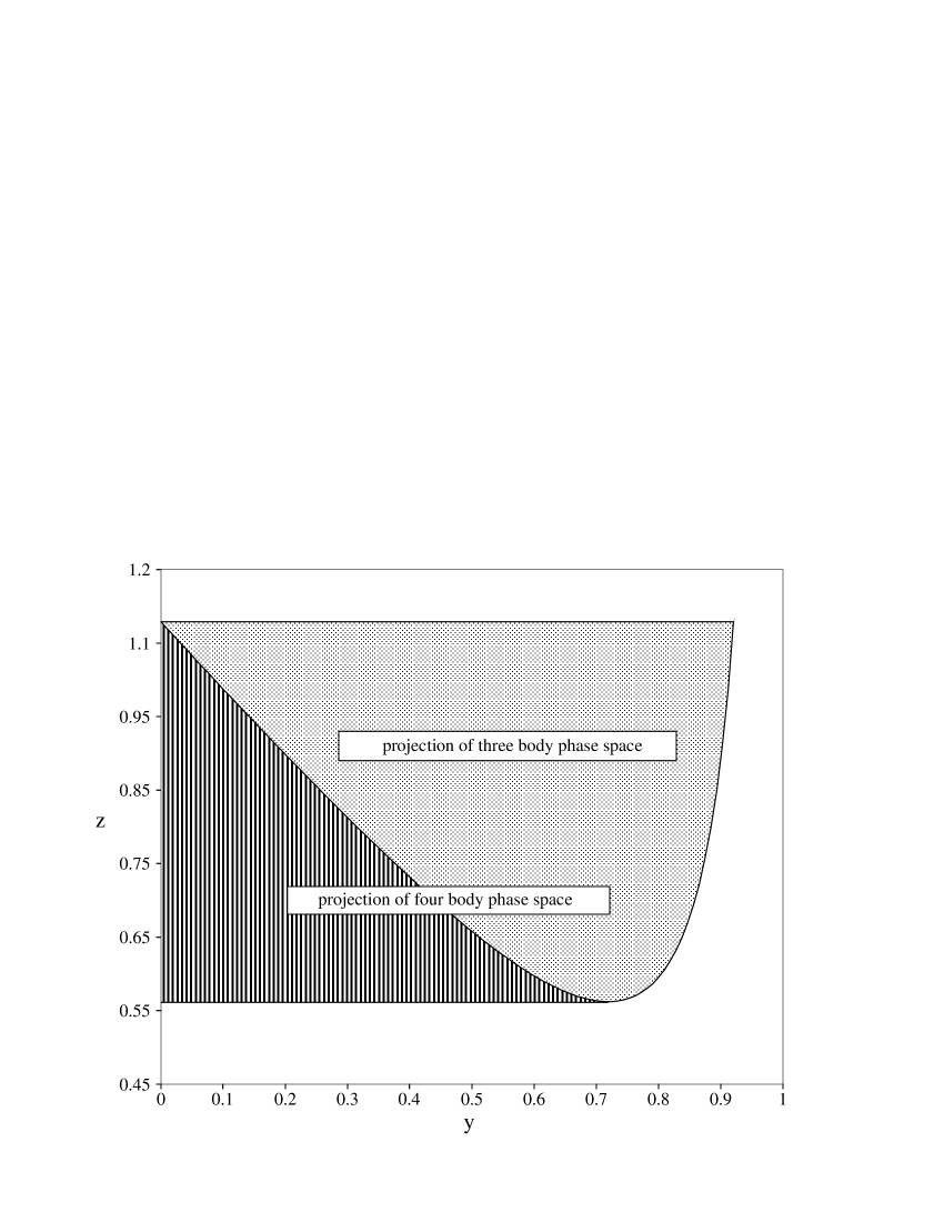
Figure 1: Dalitz plot for the three and four body final states.

This translates into the distribution

$$\rho^{\gamma}(y,z) = \frac{M_{K}}{2^{12}\pi^{5}}\int\limits_{M^{2}_{\gamma}}^{x_{\rm max}}dx\frac{1}{2\pi}\int\frac{d^{3}p_{\nu}}{p_{\nu}^{0}}\frac{d^{3}p_{\gamma}}{p_{\gamma}^{0}}$$

$$\times \delta^{(4)}(p_{K}-p_{\pi}-p_{e}-p_{\nu}-p_{\gamma})\sum_{\rm pol}|{\cal M}^{\gamma}|^{2},$$

with

$$x_{\rm max} = M_{K}^{2}\bigg{\{}1+r_{\pi}+r_{e}-y-z$$ (4.8)

$${}+\frac{1}{2}\Big{[}yz+\sqrt{(y^{2}-4r_{e})(z^{2}-4r_{\pi})}\Big{]}\bigg{\}}.$$

In (4.1) we have extended the integration over the whole range of the invariant mass of the unobserved $\nu_{e}\,\gamma$ system. The integrals occurring in (4.1) have the general form gin67

$$I_{m,n}(p_{1},p_{2};P,M_{\gamma}):=$$

$$\frac{1}{2\pi}\int\frac{d^{3}q}{q^{0}}\frac{d^{3}k}{k^{0}}\frac{\delta^{(4)}(P-q-k)}{(p_{1}\!\cdot k\!+M_{\gamma}^{2}/2)^{m}(p_{2}\!\cdot\!k+M_{\gamma}^{2}/2)^{n}}.$$

The results for these integrals in the limit $M_{\gamma}=0$ can be found in the Appendix of gin67 . Using the definition (4.1), the radiative decay distribution (4.1) can be written as gin68

$$\rho^{\gamma}(y,z)=$$

$$\frac{\alpha}{\pi}\Bigg{[}\rho^{(0)}(y,z)I_{0}(y,z;M_{\gamma})+\frac{G_{\rm F}^{2}|V_{us}|^{2}|f_{+}^{K^{0}\pi^{-}}|^{2}M_{K}}{64\pi^{3}}$$

$$\times\!\!\int\limits_{0}^{x_{\rm max}}\!\!dx\sum_{m,n}c_{m,n}I_{m,n}\Bigg{]},$$

where the infrared divergences are now confined to

$$I_{0}(y,z;M_{\gamma})=$$ (4.11)

$$\frac{1}{4}\int\limits_{M^{2}_{\gamma}}^{x_{\rm max}}dx\Big{[}2\,p_{e}\!\cdot\!p_{\pi}\,I_{1,1}(p_{e},p_{\pi};p_{K}-p_{\pi}-p_{e};M_{\gamma})$$

$$\qquad\quad{}-M_{\pi}^{2}\,I_{0,2}(p_{e},p_{\pi};p_{K}-p_{\pi}-p_{e};M_{\gamma})$$

$$\qquad\quad{}-m_{e}^{2}\,I_{2,0}(p_{e},p_{\pi};p_{K}-p_{\pi}-p_{e};M_{\gamma})\Big{]}.$$

The explicit form of the function $I_{0}$ can be found in Appendix C. The coefficients $c_{m,n}$ were given in Eq. (21) of gin68 .

Table 1: $A_{1}^{(0)}(y,z)\times 10^{2}$ for $K^{0}_{e3}$ decay

$z\backslash y$	0.05	0.15	0.25	0.35	0.45	0.55	0.65	0.75	0.85
1.05	6.54	36.54	58.54	72.54	78.54	76.54	66.54	48.54	22.54
1.00		19.54	43.54	59.54	67.54	67.54	59.54	43.54	19.54
0.95		2.54	28.54	46.54	56.54	58.54	52.54	38.54	16.54
0.90			13.54	33.54	45.54	49.54	45.54	33.54	13.54
0.85				20.54	34.54	40.54	38.54	28.54	10.54
0.80				7.54	23.54	31.54	31.54	23.54	7.54
0.75					12.54	22.54	24.54	18.54	4.54
0.70					1.54	13.54	17.54	13.54	1.54
0.65						4.54	10.54	8.54
0.60							3.54	3.54

Table 2: $[A_{1}(y,z)-A_{1}^{(0)}(y,z)]\times 10^{2}$ for $K^{0}_{e3}$ decay

$z\backslash y$	0.05	0.15	0.25	0.35	0.45	0.55	0.65	0.75	0.85
1.05	1.685	2.071	1.513	0.562	-0.523	-1.541	-2.295	-2.542	-1.864
1.00		2.188	1.999	1.243	0.237	-0.799	-1.651	-2.061	-1.582
0.95		1.775	2.024	1.464	0.562	-0.432	-1.295	-1.757	-1.356
0.90			1.844	1.524	0.749	-0.180	-1.022	-1.501	-1.140
0.85				1.476	0.856	0.012	-0.792	-1.269	-0.925
0.80				1.313	0.901	0.162	-0.589	-1.049	-0.705
0.75					0.883	0.276	-0.407	-0.839	-0.471
0.70					0.772	0.353	-0.243	-0.633	-0.200
0.65						0.384	-0.097	-0.428
0.60							0.031	-0.212

The function $\Delta^{\rm IR}$ introduced in (2.20) can now be related to $I_{0}$ by

$$\Delta^{\rm IR}(y,z)=\frac{\alpha}{\pi}\left[I_{0}(y,z;M_{\gamma})+\frac{1}{2}\Gamma(s,m^{2}_{e},M_{\pi}^{2};M_{\gamma})\right]\ .$$ (4.12)

An analytic expression of the integral occurring in the last line of (4.1) was given in Appendix B of gin70 in terms of the quantities $V_{i}$:

$$\int\limits_{0}^{x_{\rm max}}dx\>\sum_{m,n}c_{m,n}I_{m,n}=\sum_{i=0}^{7}V_{i}.$$ (4.13)

As already noticed in CKNRT02 , the quantity $J_{9}(i)$ given in Eq. (A9) of gin70 (which is needed for the evaluation of $V_{7}=U_{7}$) contains two mistakes: the plus-sign in the last line of (A9) should be replaced by a minus-sign, and $|\beta_{i}^{\rm max}|$ at the end of the first line of (A9) should simply read $\beta_{i}^{\rm max}$. The function $\Delta_{i}^{\rm IB}$ introduced in (2.20) can now be written as

$$\Delta_{1}^{\rm IB}=\frac{2\alpha}{\pi M_{K}^{4}}\sum_{i=0}^{7}V_{i}\Big{|}_{\xi=0}.$$ (4.14)

The expressions in (4.12) and (4.14) fully determine the radiatively corrected decay density $A_{1}(y,z)$ (2.20). In order to appreciate the effect of these universal long-distance corrections, we report the kinematical density $A_{1}^{(0)}$ in the absence of electromagnetism for several individual points of the Dalitz plot in Table 1, while the corresponding radiative corrections entering in (2.20) are displayed in Table 2. Note that the relative size of the electromagnetic corrections for some points (especially near the boundary) exceeds the average shift considerably. For completeness, we display a sample of numerical values for the kinematical densities (2.9) and (2.20) also for the $K^{+}_{e3}$ decay mode in Tables 3 and 4.

Table 3: $A_{1}^{(0)}(y,z)\times 10^{2}$ for $K^{+}_{e3}$ decay

$z\backslash y$	0.05	0.15	0.25	0.35	0.45	0.55	0.65	0.75	0.85
1.05	8.10	38.10	60.10	74.10	80.10	78.10	68.10	50.10	24.10
1.00		21.10	45.10	61.10	69.10	69.10	61.10	45.10	21.10
0.95		4.10	30.10	48.10	58.10	60.10	54.10	40.10	18.10
0.90			15.10	35.10	47.10	51.10	47.10	35.10	15.10
0.85			0.10	22.10	36.10	42.10	40.10	30.10	12.10
0.80				9.10	25.10	33.10	33.10	25.10	9.10
0.75					14.10	24.10	26.10	20.10	6.10
0.70					3.10	15.10	19.10	15.10	3.10
0.65						6.10	12.10	10.10	0.10
0.60							5.10	5.10
0.55								0.10

Table 4: $[A_{1}(y,z)-A_{1}^{(0)}(y,z)]\times 10^{2}$ for $K^{+}_{e3}$ decay

$z\backslash y$	0.05	0.15	0.25	0.35	0.45	0.55	0.65	0.75	0.85
1.05	1.494	1.697	1.174	0.313	-0.670	-1.593	-2.275	-2.486	-1.841
1.00		1.708	1.364	0.610	-0.320	-1.236	-1.946	-2.213	-1.638
0.95		1.558	1.378	0.732	-0.128	-1.006	-1.704	-1.983	-1.440
0.90			1.356	0.821	0.036	-0.796	-1.474	-1.758	-1.240
0.85			1.321	0.898	0.190	-0.593	-1.248	-1.533	-1.035
0.80				0.971	0.341	-0.392	-1.021	-1.305	-0.822
0.75					0.490	-0.191	-0.794	-1.075	-0.597
0.70					0.639	0.010	-0.566	-0.841	-0.348
0.65						0.214	-0.333	-0.598	-0.020
0.60							-0.094	-0.340
0.55								-0.014

4.2 Phase space integrals

Once the function $A_{1}(y,z)$ is known, the numerical coefficients $a_{0,1,2}$ entering in the phase space integral (2.24) can be calculated by integration over the Dalitz plot. These are reported in Table 5 for the $K^{0}_{e3}$ mode, while the corresponding results for $K^{+}_{e3}$ can be found in CKNRT02 . We recall once again that these numbers correspond to the specific prescription for the treatment of real photons described in the previous section: accept all pion and positron energies within the whole $K_{e3}$ Dalitz plot ${\cal D}$ and all kinematically allowed values of the Lorentz invariant $x$ defined in (4.2).

A full evaluation of the phase space factor $I_{K}$ (2.24) requires knowledge of the slope parameter. For both modes we employ the measured values PDG02 ,

$$\lambda_{+}^{K^{0}\pi^{-}} = 0.0291\pm 0.0018,$$ (4.15)

$$\lambda_{+}^{K^{+}\pi^{0}} = 0.0278\pm 0.0019.$$ (4.16)

For $K^{0}_{e3}$ decays the final numbers

$$\left.I_{K^{0}}\right|_{\alpha=0} = 0.10372,$$ (4.17)

$$I_{K^{0}} = 0.10339\pm 0.00063,$$ (4.18)

reveal that radiative corrections effectively induce a negative shift of $0.32\%$ in the factor $I_{K^{0}}$.

On the other hand, for $K^{+}_{e3}$ one finds

$$I_{K^{+}}|_{\alpha=0} = 0.10616,$$ (4.19)

$$I_{K^{+}} = 0.10482\pm 0.00067,$$ (4.20)

corresponding to a negative shift of $1.27\%$ induced by the radiative corrections. This is essentially unchanged from the analysis in CKNRT02 .

Table 5: Coefficients of the $K^{0}_{e3}$ phase space integral

	$a_{0}$	$a_{1}$	$a_{2}$
$\alpha=0$	$0.09390$	$0.3245$	$0.4485$
$\alpha\neq 0$	$0.09358$	$0.3241$	$0.4475$

5 Extraction of $|V_{us}|$ from $K^{0}_{e3}$ decays

The CKM matrix element $|V_{us}|$ can be extracted from the $K^{0}_{e3}$ decay parameters by

$$|V_{us}|=\left[\frac{128\,\pi^{3}\,\Gamma(K^{0}_{e3(\gamma)})}{G_{\rm F}^{2}\,M_{K^{0}}^{5}\,S_{\rm EW}\,I_{K^{0}}}\right]^{1/2}\cdot\frac{1}{f_{+}^{K^{0}\pi^{-}}(0)}$$ (5.1)

In spite of the unsatisfactory present status of the $K^{0}_{e3}$ data, we use them here as an illustration of the application of the above formula.

• With PDG02

  $$\Gamma(K^{0}_{e3(\gamma)})_{\rm fit}=(7.50\pm 0.08)\times 10^{6}\,{\rm s^{-1}}$$ (5.2)

  and (3.33), we find

  $$|V_{us}| = 0.2153\pm 0.0011\pm 0.0007\pm 0.0022$$ (5.3)

  $$= 0.2153\pm 0.0026,$$

  where the errors correspond to

  $$\Delta|V_{us}| = |V_{us}|\left(\pm\frac{1}{2}\frac{\Delta\Gamma}{\Gamma}\pm 0.05\cdot\frac{\Delta\lambda_{+}}{\lambda_{+}}\pm\frac{\Delta f_{+}(0)}{f_{+}(0)}\right)$$ (5.4)

  $$= |V_{us}|\big{(}\pm 0.5\%\pm 0.3\%\pm 1.0\%\big{)}.$$

• A more realistic estimate of the present $K^{0}_{e3}$ uncertainty is most probably given by PDG02

  $$\Gamma(K^{0}_{e3(\gamma)})_{\rm average}=(7.7\pm 0.5)\times 10^{6}\,{\rm s^{-1}},$$ (5.5)

  which implies

  $$|V_{us}| = 0.2182\pm 0.0071\pm 0.0007\pm 0.0022$$ (5.6)

  $$= 0.2182\pm 0.0075,$$

  corresponding to

  $$\Delta|V_{us}|=|V_{us}|\big{(}\pm 3.3\%\pm 0.3\%\pm 1.0\%\big{)}.$$ (5.7)

• Finally, combining the $K^{0}_{L}$ lifetime from the PDG with the preliminary photon-inclusive branching ratio from KLOE KLOE03 ${\rm BR}(K^{L}_{e3(\gamma)})=0.384\pm 0.002_{\rm stat.}$, we find

  $$\Gamma(K^{0}_{e3(\gamma)})_{\rm KLOE(prel.)}=(7.43\pm 0.07)\times 10^{6}\,{\rm s^{-1}},$$ (5.8)

  corresponding to

  $$|V_{us}| = 0.2143\pm 0.0010\pm 0.0007\pm 0.0022$$ (5.9)

  $$= 0.2143\pm 0.0025.$$

Since the present statistical precision is comparable to the one of the PDG fit, we expect that the experimental side of the problem will improve considerably as soon as final results from KLOE KLOE03 and NA48 NA4803 will become available.

6 Extraction of $|V_{us}|$ from $K^{+}_{e3}$ decays

In this section, we update our previous analysis of the $K^{+}_{e3}$ decay CKNRT02 in view of the new value (3.32) for the contribution of order $p^{6}$ and the recent E865 result. All other parameters of the $K^{+}_{e3}$ analysis in CKNRT02 remain essentially unchanged. Due to the inconsistency between PDG 2002 and E865 results, we analyze them separately.

• Using the PDG-fit input

  $$\Gamma(K^{+}_{e3(\gamma)})=(3.93\pm 0.05)\times 10^{6}\,{\rm s}^{-1},$$ (6.1)

  and assuming that this number refers to the inclusive width of Section 4 one obtains

  $$|V_{us}| = 0.2186\pm 0.0014\pm 0.0007\pm 0.0023$$ (6.2)

  $$= 0.2186\pm 0.0027.$$

• The $K^{+}_{e3(\gamma)}$ branching ratio measured by the E865 Collaboration E865 , when combined with the $K^{\pm}$ lifetime from the PDG, leads to the decay width

  $$\Gamma(K^{+}_{e3(\gamma)})=(4.12\pm 0.08)\times 10^{6}\,{\rm s}^{-1}.$$ (6.3)

  Note that the value ${\rm BR}(K^{+}_{e3(\gamma)})$ given in E865 contains also events outside the $K^{+}_{e3}$ Dalitz plot boundary. This additional $0.5\%$ contribution has been subtracted in (6.3) in accordance with our prescription of the treatment of real photons. Finally, we find

  $$|V_{us}| = 0.2238\pm 0.0022\pm 0.0007\pm 0.0023$$ (6.4)

  $$= 0.2238\pm 0.0033.$$

  Together with $|V_{ud}|$ and $|V_{ub}|$ as shown in (1), this number implies

  $$|V_{ud}|^{2}+|V_{us}|^{2}+|V_{ub}|^{2}-1=-0.0024\pm 0.0021,$$ (6.5)

  in rather good agreement with a unitary mixing matrix.

The sizeable disagreement between the result of E865 and the PDG-fit (from old experiments) calls for further experimental efforts in this decay channel.

7 Combined analysis of $K^{0}_{e3}$ and $K^{+}_{e3}$ data

$K^{+}_{e3}$ and $K^{0}_{e3}$ branching fractions allow for two independent determinations of $f_{+}^{K^{0}\pi^{-}}(0)\cdot|V_{us}|$, provided one brings under theoretical control isospin breaking in the ratio of form factors at $t=0$,

$$r_{+0}:=f_{+}^{K^{+}\pi^{0}}(0)\Big{/}f_{+}^{K^{0}\pi^{-}}(0).$$ (7.1)

The standard model allows a remarkably precise prediction of this quantity. The contributions of order $p^{6}$ as well as the couplings $X_{6}$ and $K_{12}$ cancel and we are left with the expression

$$r_{+0}^{\rm th} = 1+\sqrt{3}\left(\varepsilon^{(2)}+\varepsilon^{(4)}_{\rm S}+\varepsilon^{(4)}_{\rm EM}\right)$$ (7.2)

$${}-\frac{\alpha}{4\pi}\log\frac{M^{2}_{K^{\pm}}}{M^{2}_{\pi^{\pm}}}-16\pi\alpha X_{1}+\dots$$

$${}=1.022\pm 0.003-16\pi\alpha X_{1},$$

where the ellipses in the second line stand for isospin violating corrections arising at ${\cal O}((m_{d}-m_{u})p^{4},e^{2}p^{4})$ in the chiral expansion. We expect them to shift the result at most by $10^{-3}$. Also these not yet determined contributions have been accounted for in the error given in the last line of (7.2). Although no theoretical estimate of the coupling $X_{1}$ is presently available, there is no reason why this low energy constant should lie outside the range suggested by naive dimensional analysis (3.18). Already such a rough estimate of $X_{1}$ shows that $r_{+0}$ is confined to the rather narrow band

$$1.017\leq r_{+0}^{\rm th}\leq 1.027.$$ (7.3)

We emphasize that sizeable deviations from this predicted range could only be understood as (i) failure of naive dimensional analysis for $X_{1}$ (and a dramatic one) or (ii) failure of chiral power counting.

On the other hand, the ratio (7.1) is related to the observable

$$r_{+0}^{\rm exp}=\left(\frac{2\,\Gamma(K^{+}_{e3(\gamma)})\,M_{K^{0}}^{5}\,I_{K^{0}}}{\Gamma(K^{0}_{e3(\gamma)})\,M_{K^{+}}^{5}\,I_{K^{+}}}\right)^{1/2},$$ (7.4)

with the caveat that the phase space factors $I_{K}$ be evaluated according to the same prescription for real photons adopted in measuring $\Gamma(K_{e3(\gamma)})$. Once again, it is instructive to consider several cases:

• Using (5.2) and (6.3), we find

  $$r_{+0}^{\rm exp} = 1.062\pm 0.010\pm 0.006\pm 0.003\pm 0.003$$ (7.5)

  $$= 1.062\pm 0.013,$$

  where the errors given in the first line refer to the experimental uncertainties of $\Gamma(K^{+}_{e3(\gamma)})$, $\Gamma(K^{0}_{e3(\gamma)})$, $\lambda_{+}^{K^{+}\pi^{0}}$ and $\lambda_{+}^{K^{0}\pi^{-}}$, respectively. The outcome is clearly in conflict with the prediction (7.3) of the standard model and indicates indeed an inconsistency of the present $K^{+}_{e3}$ and $K^{0}_{e3}$ data. This is also illustrated by Fig. 2 where data data from $K^{+}_{e3}$ (E865) and $K^{0}_{e3}$ (PDG-fit), after using $r_{+0}^{\rm th}$ as discussed above, lead to two inconsistent determinations of the product $f_{+}^{K^{0}\pi^{-}}(0)\cdot|V_{us}|$.

• Taking (5.5) instead of (5.2), the resulting numbers are

  $$r_{+0}^{\rm exp} = 1.049\pm 0.010\pm 0.034\pm 0.003\pm 0.003$$ (7.6)

  $$= 1.049\pm 0.036.$$

  This value is consistent with (7.3) however with a large error caused by the big uncertainty in (5.5).

• The inconsistency is somehow mitigated when one uses the present PDG-fit entries for both $K^{+}_{e3}$ and $K^{0}_{e3}$, leading to

  $$r_{+0}^{\rm exp} = 1.038\pm 0.006\pm 0.006\pm 0.003\pm 0.003$$ (7.7)

  $$= 1.038\pm 0.010.$$

The present confusing status is summarized in Figure 2, where we plot $f_{+}^{K^{0}\pi^{-}}(0)\cdot|V_{us}|$ as determined from different $K^{+}_{e3}$ and $K^{0}_{e3}$ experimental input. The points corresponding to $K^{+}_{e3}$ have been obtained by using the central value for $r_{+0}^{\rm th}$. The overall $0.78\%$ normalization uncertainty of these points is not reported in the plot.

Figure 2: $|V_{us}|\cdot f_{+}^{K^{0}\pi^{-}}(0)$ from $K_{e3}$ modes (see text for details). The KLOE result is preliminary and the quoted error is statistical only KLOE03 .

For the analysis of forthcoming high-precision data on $K_{e3}$ decays we propose the following strategy:

• Check the consistency of $K^{+}_{e3}$ and $K^{0}_{e3}$ data by comparing $r_{+0}^{\rm exp}$ with the theoretically allowed range (7.3).

• Determine the low energy constant $X_{1}$ from $r_{+0}^{\rm exp}$ by inverting (7.2),

  $$X_{1}=\frac{1.022\pm 0.003({\rm theor.})-r_{+0}^{\rm exp}}{16\pi\alpha}.$$ (7.8)

  (We refrain from extracting a number for $X_{1}$ based on the present data as they are apparently inconsistent.)

• Recalculate $\widehat{f}_{+}^{K^{0}\pi^{-}}$ from (3.5) by using the experimentally determined parameter $X_{1}$.

• Use the new number for $f_{+}^{K^{0}\pi^{-}}(0)$ in the determination of $|V_{us}|$ as described in Sect. 5.

• Finally, one can also use the experimentally determined $X_{1}$ to improve radiative corrections to the pion beta decay pibeta , relevant for the extraction of $|V_{ud}|$ from this mode once the PIBETA experiment finalizes the analysis pibetaexp .

8 Conclusions

In this work, we have studied $K_{e3}$ decays using chiral perturbation theory with virtual photons and leptons. This method allows a unified and consistent treatment of strong and electromagnetic contributions to the decay amplitudes within the standard model. We have considered strong effects up to ${\cal O}(p^{6})$ in the chiral expansion. Isospin breaking due to the mass difference of the light quarks has been included up to the order $(m_{d}-m_{u})p^{2}$. Electromagnetic effects were taken into account up to ${\cal O}(e^{2}p^{2})$. The largest theoretical error is generated by the contribution of ${\cal O}(p^{6})$ inducing a $1\%$ uncertainty in the determination of the $K_{e3}$ form factors. Additional theoretical investigation is needed to increase our confidence in the estimate of local contributions at ${\cal O}(p^{6})$.

Based on our theoretical results, we have described the extraction of the CKM matrix element $|V_{us}|$ from experimental decay parameters and a consistency check of $K_{e3}^{+}$ and $K_{e3}^{0}$ data.

Using the recent E865 result on the $K_{e3}^{+}$ branching ratio, we find

$$|V_{us}|=0.2238\pm 0.0033,$$ (8.1)

being perfectly consistent with CKM unitarity. It should be noted, however, that the E865 ratio differs from older $K_{e3}^{+}$ measurements by 2.3 $\sigma$. Furthermore, the E865 result and the present $K_{e3}^{0}$ rate as given by PDG 2002 (based on very old data) and by KLOE preliminary results can hardly be reconciled within the framework of the standard model. Recently-completed or ongoing experiments will help to clarify the situation.

Finally a short remark on $|V_{ud}|$, the second important source of information for the check of CKM unitarity: the present number for $|V_{ud}|$ is extracted from super-allowed Fermi transitions and neutron beta decay. In principle, the pionic beta decay ($\pi_{e3}$) provides a unique test of these existing determinations. This decay mode is theoretically extremely clean pibeta and also completely consistent with the present analysis of $K_{e3}$ decays. Using the present result on the $\pi_{e3}$ branching ratio from the PIBETA experiment pibetaexp , one finds

$$|V_{ud}|=0.9716\pm 0.0039,$$ (8.2)

to be compared with the current PDG value shown in (1). The final result from this experiment is expected to reach a precision for the pion beta decay rate of about $0.5\%$. Further efforts for an improvement of the experimental accuracy of $\pi_{e3}$ would be highly desirable.

Acknowledgements. We thank J. Bijnens, G. Ecker, J. Gasser and H. Leutwyler for useful remarks. We have profited from discussions with G. Isidori, B. Sciascia, T. Spadaro and J. Thompson. V. C. is supported by a Sherman Fairchild fellowship from Caltech.

Appendix

Appendix A Photonic Loop Functions

The photonic loop contributions to the $K_{\ell 3}$ form factors depend on the charged lepton and meson masses $m_{\ell}^{2}$, $M^{2}$, as well as on the Mandelstam variables $u=(p_{K}-p_{\ell})^{2}$ (for $K^{+}_{\ell 3}$ decays) and $s=(p_{\pi}+p_{\ell})^{2}$ (for $K^{0}_{\ell 3}$ decays). In what follows we denote by $v$ the Mandelstam variable appropriate to each decay. In order to express the loop functions in a compact way, it is useful to define the following intermediate variables:

$$R=\frac{m_{\ell}^{2}}{M^{2}},\ \ Y=1+R-\frac{v}{M^{2}},\ \ X=\frac{Y-\sqrt{Y^{2}-4R}}{2\sqrt{R}}.$$ (A.1)

In terms of such variables and of the dilogarithm

$${\rm Li}_{2}(x)=-\int_{0}^{1}\frac{dt}{t}\log(1-xt),$$ (A.2)

the functions contributing to $\Gamma(v,m_{\ell}^{2},M^{2};M_{\gamma})$ are given by CKNRT02

$$\Gamma_{c}(v,m_{\ell}^{2},M^{2};M_{\gamma})=2M^{2}Y\,{\cal C}(v,m_{\ell}^{2},M^{2})$$ (A.3)

$${}+2\log\frac{Mm_{\ell}}{M_{\gamma}^{2}}\bigg{(}1+\frac{XY\log X}{\sqrt{R}(1-X^{2})}\bigg{)}.$$

$${\cal C}(v,m_{\ell}^{2},M^{2})=\frac{1}{m_{\ell}M}\frac{X}{1-X^{2}}$$

$$\times \left[-\frac{1}{2}\log^{2}X+2\log X\log(1-X^{2})-\frac{\pi^{2}}{6}+\frac{1}{8}\log^{2}R\right.$$

$${}+\left.{\rm Li}_{2}(X^{2})+{\rm Li}_{2}(1-\frac{X}{\sqrt{R}})+{\rm Li}_{2}(1-X\sqrt{R})\right],$$

$$\Gamma_{1}(v,m_{\ell}^{2},M^{2}) = \frac{1}{2}\Big{[}-\,\log R\,+\,(4-3Y){\cal F}(v,m_{\ell}^{2},M^{2})\Big{]}$$

$$\Gamma_{2}(v,m_{\ell}^{2},M^{2}) = \frac{1}{2}\Big{(}1-\frac{m_{\ell}^{2}}{v}\Big{)}\Big{[}-{\cal F}(v,m_{\ell}^{2},M^{2})(1-R)$$ (A.5)

$$+ \log R\Big{]}-\frac{1}{2}(3-Y){\cal F}(v,m_{\ell}^{2},M^{2})\,,$$

and

$${\cal F}(v,m_{\ell}^{2},M^{2})\,=\,\frac{2}{\sqrt{R}}\,\frac{X}{1-X^{2}}\,\log X\,.$$ (A.6)

Appendix B Mesonic Loop Functions

The loop function $H_{PQ}(t)$ gl852 ; GL85 is given by

$$H_{PQ}(t)=\displaystyle\frac{1}{F_{0}^{2}}\bigg{[}h_{PQ}^{r}(t,\mu)+\frac{2}{3}tL_{9}^{r}(\mu)\bigg{]},$$ (B.1)

where

$$h_{PQ}^{r}(t,\mu) = \frac{1}{12t}\lambda(t,M_{P}^{2},M_{Q}^{2})\,\bar{J}_{PQ}(t)$$ (B.2)

$${}+\frac{1}{18(4\pi)^{2}}(t-3\Sigma_{PQ})$$

$${}-\frac{1}{12}\bigg{\{}\frac{2\Sigma_{PQ}-t}{\Delta_{PQ}}[A_{P}(\mu)-A_{Q}(\mu)]$$

$$\qquad{}-2[A_{P}(\mu)+A_{Q}(\mu)]\bigg{\}},$$

with

$$\lambda(x,y,z)=x^{2}+y^{2}+z^{2}-2(xy+xz+yz),$$ (B.3)

$$\Sigma_{PQ}=M_{P}^{2}+M_{Q}^{2},\qquad\Delta_{PQ}=M_{P}^{2}-M_{Q}^{2},$$ (B.4)

$$A_{P}(\mu)=-\frac{M_{P}^{2}}{(4\pi)^{2}}\log\frac{M_{P}^{2}}{\mu^{2}},$$ (B.5)

and

$$\bar{J}_{PQ}(t)=\frac{1}{32\pi^{2}}\Bigg{[}2+\frac{\Delta_{PQ}}{t}\log\frac{M_{Q}^{2}}{M_{P}^{2}}-\frac{\Sigma_{PQ}}{\Delta_{PQ}}\log\frac{M_{Q}^{2}}{M_{P}^{2}}$$ (B.6)

$${}-\frac{\lambda^{1/2}(t,M_{P}^{2},M_{Q}^{2})}{t}$$

$$\times\log\left(\frac{[t+\lambda^{1/2}(t,M_{P}^{2},M_{Q}^{2})]^{2}-\Delta_{PQ}^{2}}{[t-\lambda^{1/2}(t,M_{P}^{2},M_{Q}^{2})]^{2}-\Delta_{PQ}^{2}}\right)\Bigg{]}.$$

The quantity $H_{PQ}(0)$ appearing in the evaluation of $f_{+}(0)$ is given by gl852

$$H_{PQ}(0) = -\frac{1}{128\pi^{2}F_{0}^{2}}(M_{P}^{2}+M_{Q}^{2})\,h_{0}\!\left(\frac{M_{P}^{2}}{M_{Q}^{2}}\right),$$

$$h_{0}(x) = 1+\frac{2x}{1-x^{2}}\log x.$$ (B.7)

For the theoretical determination of the slope parameter one needs the derivative of the function $H_{PQ}(t)$ at $t=0$ given by gl852

$$\left.\frac{dH_{PQ}(t)}{dt}\right|_{t=0} = \frac{2}{3F_{0}^{2}}\left\{L_{9}^{r}(\mu)-\frac{1}{128\pi^{2}}\log\frac{M_{P}M_{Q}}{\mu^{2}}\right\}$$

$${}-\frac{1}{192\pi^{2}F_{0}^{2}}\,h_{1}\!\left(\frac{M_{P}^{2}}{M_{Q}^{2}}\right),$$

$$h_{1}(x) = \frac{x^{3}-3x^{2}-3x+1}{2(x-1)^{3}}\log x$$ (B.8)

$${}+\frac{1}{2}\left(\frac{x+1}{x-1}\right)^{2}-\frac{1}{3}.$$

Appendix C The function $I_{0}(y,z;M_{\gamma})$ for $K^{0}_{\ell 3}$

The analytic result for the integral $I_{0}(y,z;M_{\gamma})$ defined in (4.11) is given by

$$I_{0}(y,z;M_{\gamma})=\frac{1}{2\beta}\log\frac{1+\beta}{1-\beta}\log\frac{2\beta p_{\ell}\!\cdot\!p_{\pi}}{M_{\gamma}^{2}}-\log\frac{m_{\ell}M_{\pi}}{M_{\gamma}^{2}}$$ (C.1)

$${}+\frac{1}{2\beta}\log\frac{1+\beta}{1-\beta}\log\frac{2\beta\gamma(p_{\ell}\!\cdot\!p_{\pi})^{2}\left(1-\tau(0)^{2}\right)^{2}}{P\!\cdot\!p_{\ell}P\!\cdot\!p_{\pi}}$$

$${}+\frac{1}{2\beta}\big{[}-{\rm Li}_{2}(\eta_{1})+{\rm Li}_{2}(1/\eta_{1})-{\rm Li}_{2}(\eta_{2})+{\rm Li}_{2}(1/\eta_{2})\big{]}$$

$${}+\frac{2}{\beta}\bigg{[}\log\tau(x_{\rm max})\log\frac{1-\tau(0)\tau(x_{\rm max})}{1-\tau(x_{\rm max})/\tau(0)}$$

$${}+{\rm Li}_{2}\big{(}\tau(x_{\rm max})\tau(0)\big{)}-{\rm Li}_{2}\big{(}\tau(x_{\rm max})/\tau(0)\big{)}$$

$${}-{\rm Li}_{2}\left(\tau(0)^{2}\right)+\pi^{2}/6\bigg{]}$$

$${}+\left({\rm arcosh}\frac{p_{\ell}\!\cdot\!p_{\pi}+x_{\rm max}/2}{m_{\ell}M_{\pi}}\right)^{2}-\left({\rm arcosh}\frac{p_{\ell}\!\cdot\!p_{\pi}}{m_{\ell}M_{\pi}}\right)^{2}$$

$${}+\log\frac{4\,P\!\cdot\!p_{\ell}\,P\!\cdot\!p_{\pi}}{x_{\rm max}^{2}},$$

where

$$\beta = \frac{\sqrt{(p_{\ell}\!\cdot\!p_{\pi})^{2}-m_{\ell}^{2}M_{\pi}^{2}}}{p_{\ell}\!\cdot\!p_{\pi}},$$ (C.2)

$$\gamma = \frac{P\!\cdot\!p_{\ell}\,P\!\cdot\!p_{\pi}}{p_{\ell}\!\cdot\!p_{\pi}}$$

$$\times \frac{(p_{\ell}\!\cdot\!p_{\pi})^{2}-m_{\ell}^{2}M_{\pi}^{2}}{2\,p_{\ell}\!\cdot\!p_{\pi}\,P\!\cdot\!p_{\ell}\,P\!\cdot\!p_{\pi}-m_{\ell}^{2}(P\!\cdot\!p_{\pi})^{2}-M_{\pi}^{2}(P\!\cdot\!p_{\ell})^{2}},$$

$$P = p_{K}-p_{\pi}-p_{\ell}$$ (C.4)

$$\eta_{1,2} = \frac{1-2\gamma\pm\sqrt{\beta^{2}+4\gamma^{2}-4\gamma}}{1+\beta},$$ (C.5)

$$\tau(x) = \frac{p_{\ell}\!\cdot\!p_{\pi}+x/2-\sqrt{(p_{\ell}\!\cdot\!p_{\pi}+x/2)^{2}-m_{\ell}^{2}M_{\pi}^{2}}}{m_{\ell}M_{\pi}}.$$ (C.6)

References

- (1) The Particle Data Group, K. Hagiwara et al., Phys. Rev. D 66, 010001-1 (2002)
- (2) A. Sher et al., hep-ex/0305042
- (3) V. Cirigliano, M. Knecht, H. Neufeld, H. Rupertsberger, P. Talavera, Eur. Phys. J. C 23, 121 (2002)
- (4) M. Knecht, H. Neufeld, H. Rupertsberger, P. Talavera, Eur. Phys. J. C 12, 469 (2000)
- (5) W.J. Marciano, A. Sirlin, Phys. Rev. Lett. 71, 3629 (1993)
- (6) J. Bijnens, P. Talavera, Nucl. Phys. B 669, 341 (2003)
- (7) J. Gasser, H. Leutwyler, Nucl. Phys. B 250, 517 (1985)
- (8) P. Post, K. Schilcher, Eur. Phys. J. C 25, 427 (2002)
- (9) J. Gasser, H. Leutwyler, Nucl. Phys. B 250, 465 (1985)
- (10) R. Urech, Nucl. Phys. B 433, 234 (1995)
- (11) H. Neufeld, H. Rupertsberger, Z. Phys. C 68, 91 (1995)
- (12) H. Neufeld, H. Rupertsberger, Z. Phys. C 71, 131 (1996)
- (13) J. Bijnens, G. Colangelo, G. Ecker, JHEP 02, 020 (1999)
- (14) J. Bijnens, G. Colangelo, G. Ecker, Ann. Phys. 280, 100 (2000)
- (15) H. Leutwyler, Phys. Lett. B 378, 313 (1996)
- (16) G. Amorós, J. Bijnens, P. Talavera, Nucl. Phys. B 602, 87 (2001)
- (17) J. Bijnens, J. Prades, Nucl. Phys. B 490, 239 (1997)
- (18) B. Moussallam, Nucl. Phys. B 504, 381 (1997)
- (19) H. Leutwyler, M. Roos, Z. Phys. C 25, 91 (1984)
- (20) M. Jamin, J. A. Oller, A. Pich, hep-ph/0401080
- (21) V. Cirigliano, A. Pich, G. Ecker, H. Neufeld, JHEP 06, 012 (2003)
- (22) A. Pich, hep-ph/0205030
- (23) V. Cirigliano, eConf C0304052, WG603 (2003)
- (24) E.S. Ginsberg, Phys. Rev. 162, 1570 (1967); ibid. 187, 2280(E) (1969)
- (25) E.S. Ginsberg, Phys. Rev. 171, 1675 (1968); ibid. 174, 2169(E) (1968); ibid. 187, 2280(E) (1969)
- (26) E.S. Ginsberg, Phys. Rev. D 1, 229 (1970)
- (27) B. Sciascia (KLOE Coll.), eConf C0304052, WG607 (2003)
- (28) D. Madigozhin (NA48/2 Coll.), eConf C0304052, WG605 (2003)
- (29) G. Calderon, G. Lopez Castro, Phys. Rev. D 65, 073032 (2002)
- (30) G. Isidori, eConf C0304052, WG601 (2003)
- (31) V. Cirigliano, M. Knecht, H. Neufeld, H. Pichl, Eur. Phys. J. C 27, 255 (2003)
- (32) D. Počanić et al. (PIBETA Coll.), hep-ex/0312030