$n$-Particle irreducible effective action techniques for gauge theories

A loop or coupling expansion of a so-called $n$-particle irreducible ($n$PI) generating functional provides a well-defined approximation scheme in terms of self-consistently dressed propagators and $n$-point vertices. A self-consistently complete description determines the functional for arbitrarily high $n$ to a given order in the expansion. We point out an equivalence hierarchy for $n$PI effective actions, which allows one to obtain a self-consistently complete result in practice. The method is applied to a $SU(N)$ gauge theory with fermions up to four-loop or ${\mathcal{O}}(g^{6})$ corrections. For non-equilibrium we discuss the connection to kinetic theory. The leading-order on-shell results in $g$ can be obtained from the three-loop effective action approximation, which already includes in particular all diagrams enhanced by the Landau Pomeranchuk Migdal effect. Furthermore, we compare the effective action approach with Schwinger-Dyson (SD) equations. By construction, SD equations are expressed in terms of loop diagrams including both classical and dressed vertices, which leads to ambiguities of whether classical or dressed ones should be employed at a given truncation order. We point out that these problems are absent using effective action techniques. We show that a wide class of truncations of SD equations cannot be obtained from the $n$PI effective action. In turn, our results can be used to resolve SD ambiguities of whether classical or dressed vertices should be employed at a given truncation order.

1 Introduction and overview

1.1 Background

Selective summation to infinite order in perturbation theory often plays an important role in vacuum, thermal equilibrium or nonequilibrium quantum field theory. A prominent example in high temperature field theory is the so-called “hard-thermal-loop” (HTL) perturbation theory [1]. For small coupling $g\ll 1$ the description of gauge boson excitations with wave number $k\sim gT$ requires appropriately resummed propagators and vertices. After the selective HTL resummation the effective interactions among the $gT$ scale degrees of freedom are weak and may be treated perturbatively. However, for excitations with wave number $k\sim g^{2}T$ the occupation numbers of individual modes can grow nonperturbatively large $\sim 1/g^{2}$ and the perturbative treatment breaks down.

For out-of-equilibrium situations there are additional complications which do not appear in vacuum or thermal equilibrium. Nonequilibrium dynamics typically poses an initial value problem: time-translation invariance is explicitly broken by the presence of the initial time, where the system has been prepared. During the nonequilibrium evolution the system may effectively loose the dependence on the details of the initial condition, and become approximately time-translation invariant for sufficiently late times. If thermal equilibrium is approached then the late-time result is universal in the sense that it becomes uniquely determined by the values of the (conserved) energy density and of possible conserved charges. It is well-known that the late-time behavior of quantum fields cannot be described using standard perturbation theory. The perturbative time evolution suffers from the presence of spurious, so-called secular terms, which grow with time and invalidate the expansion even in the presence of a weak coupling. Here it is important to note that the very same problem can appear as well for nonperturbative approximation schemes such as $1/N$ expansions [2].

It has recently been demonstrated for scalar [3, 4, 5, 6, 7, 8] and fermionic [9] theories that nonequilibrium dynamics with subsequent late-time thermalization can be described from a selective summation of powers of the coupling or $1/N$ without further assumptions. This provides an efficient solution to the problem of a universal late-time behavior as well as the secularity problem. These approximations are expressed in terms of a loop [10] or $1/N$ [4, 11] expansion of the so-called two-particle irreducible (2PI) effective action [12]. Though other resummations may be invoked to circumvent secular behavior of perturbative treatments (cf. e.g. [13]), the description of a universal late-time behavior poses rather strong restrictions on the possible approximations. The 2PI schemes seem to be uniquely suitable in nonequilibrium quantum field theory to capture the effective loss of initial condition details leading to thermalization. The remarkably good convergence properties of the approach have also been observed in the context of classical statistical field theories, where comparisons with exact results are possible [5]. The expansions do not rely on small departures from equilibrium, or sufficient space-time homogeneity of the system underlying effective kinetic descriptions in terms of “quasiparticles” [16]. However, 2PI effective action techniques can be very efficient in deriving kinetic equations [17, 18, 19, 16, 20].

The 2PI expansions are known to be “conserving” [12, 21], i.e. they are consistent with global symmetries of the Lagrangian [22]. In particular, energy conservation and the absence of an irreversible dynamics are viable ingredients for a description of nonequilibrium time evolution from first principles. However, these approximations can violate Ward identities associated to local symmetries, which has recently been explored and shown to be suppressed with respect to naive estimates based on power counting [23]. First applications in gauge theories use the 2PI effective action as an efficient starting point for the development of selective summation schemes for the description of the equilibrium thermodynamics of the quark-gluon plasma [24, 25] (cf. also [26]).

1.2 Equivalence hierarchy for $n$PI effective actions

To understand the success and, more importantly, the limitations of expansion schemes based on the 2PI effective action we consider in this paper so-called “$n$PI” effective actions for $n>2$. Recall that the description of the 2PI effective action $\Gamma[\phi,D]$ employs a self-consistently dressed one-point function $\phi$ and two-point function $D$: The field expectation value $\phi=\langle\varphi\rangle$ and connected propagator $D=\langle T\varphi\varphi\rangle-\phi\phi$ are dressed by solving the equations of motion $\delta\Gamma/\delta\phi=0$ and $\delta\Gamma/\delta D=0$ for a given order in the (e.g. loop) expansion of $\Gamma[\phi,D]$ [10]. However, the 2PI effective action does not treat the higher $n$-point functions with $n>2$ on the same footing as the lower ones: The three- and four-point function etc. are not self-consistently dressed in general, i.e. the corresponding proper three-vertex $V_{3}$ and four-vertex $V_{4}$ are given by the classical ones. In contrast, the $n$PI effective action $\Gamma[\phi,D,V_{3},V_{4},\ldots,V_{n}]$ provides a dressed description for the proper vertices $V_{3},V_{4},\ldots,V_{n}$ as well, with $\delta\Gamma/\delta V_{3}=0,\delta\Gamma/\delta V_{4}=0,\ldots,\delta\Gamma/\delta V_{n}=0$.

For applications it can be desirable to obtain a self-consistently complete description, which to a given order in the expansion determines $\Gamma[\phi,D,V_{3},V_{4},\ldots,V_{n}]$ for arbitrarily high $n$. Despite the complexity of a general $n$PI effective action it is important to note that a systematic, e.g. loop or coupling expansion can be nevertheless performed in practice. We point out that a self-consistently complete loop-expansion of the effective action can be based on the following equivalence hierarchy:

$$\Gamma^{\rm(1loop)}[\phi] \!=\! \Gamma^{\rm(1loop)}[\phi,D]=\ldots\,,$$

$$\Gamma^{\rm(2loop)}[\phi] \!\not=\! \Gamma^{\rm(2loop)}[\phi,D]=\Gamma^{\rm(2loop)}[\phi,D,V_{3}]=\ldots\,,$$ (1.1)

$$\Gamma^{\rm(3loop)}[\phi] \!\not=\! \Gamma^{\rm(3loop)}[\phi,D]\not=\Gamma^{\rm(3loop)}[\phi,D,V_{3}]=\Gamma^{\rm(3loop)}[\phi,D,V_{3},V_{4}]=\ldots\,,$$

where $\Gamma^{{\rm(}n{\rm-loop)}}$ denotes the approximation of the respective effective action to $n$-th loop order in the absence of sources. As a consequence, for a theory as e.g. quantum electrodynamics (QED) or chromodynamics (QCD) the 2PI effective action provides a self-consistently complete description to two-loop order or ${\mathcal{O}}(g^{2})$: For a two-loop approximation all $n$PI descriptions with $n\geq 2$ are equivalent and the 2PI effective action captures already the complete answer for the self-consistent description up to this order. In contrast, a self-consistently complete result to three-loop order or ${\mathcal{O}}(g^{4})$ requires at least the 3PI effective action etc. This hierarchy clarifies a number of questions in the literature about the success or insufficiency of expansion schemes based on the 2PI effective action:

i) Recently, it was argued that for high temperature gauge theories a loop-expansion of the 2PI effective action is not suitable for a quantitative description of transport coefficients in the context of kinetic theory [28]. As an example, the calculation of shear viscosity in a theory like QCD may be based on the inclusion of an infinite series of 2PI “ladder” diagrams in order to recover the leading order “on-shell” results in $g$ [29]. The enhancement of the infinite series of apparently higher order diagrams can be understood as a manifestation of the Landau Pomeranchuk Migdal (LPM) effect [30]. As pointed out above, for gauge theories such as QCD the 2PI effective action provides a self-consistently complete description to two-loop order or ${\mathcal{O}}(g^{2})$. However, to go beyond that order in this scheme requires to consider higher effective actions. 4PI effective actions for scalar field theories have been derived previously in Ref. [31]. In Ref. [32] the thermodynamic potential for QED with a full three-vertex was constructed, and a perturbative construction scheme for the 4PI effective action in QCD was given. We derive the 4PI effective action for a nonabelian $SU(N)$ gauge theory with fermions up to four-loop or ${\mathcal{O}}(g^{6})$ corrections, starting from the 2PI effective action and doing subsequent Legendre transforms (Sects. 2,3). The class of models include gauge theories such as QCD or abelian theories as QED, as well as simple scalar field theories with cubic or quartic interactions. For non-equilibrium (Sec. 5) we discuss the connection to kinetic theory in QED (Sec. 6). We will see that, since the lowest order contribution to the kinetic equation is of ${\mathcal{O}}(g^{4})$, the 3PI effective action provides a self-consistently complete starting point for its description. In particular, the leading-order on-shell result in $g$ can be efficiently obtained from the 3PI effective action to three-loops, which includes in particular all diagrams enhanced by the LPM effect.

ii) In nonequilibrium quantum field theory the success of the 2PI effective action to describe a universal late-time behavior (cf. Sec. 1.1) crucially depends on the self-consistent nature of the employed approximation scheme. We note that the successful descriptions of thermalization in scalar [3] and fermionic theories [9] based on a 2PI loop expansion were self-consistently complete in the above sense: We show in Sec. 2 that in the absence of a three-vertex and spontaneous symmetry breaking, to three-loop order the 2PI effective action already contains the complete answer for the self-consistent description up to this order: $\Gamma^{\rm(3loop)}[\phi=0,D]=\Gamma^{\rm(3loop)}[\phi=0,D,V_{3}=0,V_{4}]$. In the presence of (effective) cubic interactions the three-vertex would receive further corrections from the 3PI effective action.

iii) The evolution equations, which are obtained by variation of the $n$PI effective action, are closely related to Schwinger-Dyson (SD) equations [33]. Without approximations the equations of motion obtained from an exact $n$PI effective action and the exact SD equations have to agree since one can always map identities onto each other. However, in general this is no longer the case for a given order in the loop or coupling expansion of the $n$PI effective action. By construction, SD equations are expressed in terms of loop diagrams including both classical and dressed vertices, which leads to ambiguities of whether classical or dressed ones should be employed at a given truncation order. In particular, SD equations are not closed a priori in the sense that the equation for a given $n$-point function always involves information about $m$-point functions with $m>n$.

We point out that these problems are absent using effective action techniques (Sec. 4). In turn, we show that a wide class of truncations of exact SD equations cannot be obtained from the $n$PI effective action. In particular, our results can be used to resolve ambiguities of whether classical or dressed vertices should be employed for a given truncation of a SD equation. For instance, in QCD the three-loop effective action result leads to evolution equations, which are equivalent to the SD equation for the two-point function and the one-loop three-point function if  all vertices in loop-diagrams for the latter are replaced by the full vertices at that order As mentioned above the “conserving” property of using an effective action truncation can have important advantages, in particular if applied to nonequilibrium time evolution problems, where the presence of basic constants of motion such as energy conservation is crucial. SD equations have been frequently applied to nonperturbative strong interaction physics and, for instance, recent comparisons of certain approximations with gauge-fixed lattice results are encouraging [35], also for effective action techniques.

2 Higher effective actions

All information about the quantum theory can be obtained from the effective action, which is a generating functional for Green’s functions. Typically, the (1PI) effective action $\Gamma[\phi]$ is represented as a functional of the — bosonic or fermionic — field expectation value or one-point function $\phi$ only. In contrast, the so-called 2PI effective action $\Gamma[\phi,D]$ is conventionally written as a functional of $\phi$ and the full propagator or connected two-point function $D$ [12, 10]. The latter provides an efficient description of quantum corrections in terms of loop-diagrams with dressed propagator lines and classical vertices. The functional dependence of higher effective actions take into account as well the dressed three-point function, four-point function etc. or, equivalently, the proper three-vertex $V_{3}$, four-vertex $V_{4}$ and so on [31, 17]. The name “3PI” effective action is used to denote $\Gamma[\phi,D,V_{3}]$, and “4PI” refers to $\Gamma[\phi,D,V_{3},V_{4}]$ and similarly for even higher effective actions. The functionals are constructed such that the equations of motion for the respective “field variables” are obtained from stationarity conditions:

$$\frac{\delta\Gamma[\phi]}{\delta\phi}=0$$ (2.2)

for the 1PI effective action, and

$$\frac{\delta\Gamma[\phi,D]}{\delta\phi}=0\quad,\quad\frac{\delta\Gamma[\phi,D]}{\delta D}=0$$ (2.3)

for the 2PI action in the absence of sources, etc.

All functional representations of the effective action are equivalent in the sense that they are generating functionals for Green’s functions including all quantum/statistical fluctuations and, in the absence of sources, have to agree by construction:

$$\Gamma[\phi]=\Gamma[\phi,D]=\Gamma[\phi,D,V_{3}]=\Gamma[\phi,D,V_{3},V_{4}]=\Gamma[\phi,D,V_{3},V_{4},\ldots,V_{n}]$$ (2.4)

for arbitrary $n$ without further approximations. However, e.g. loop expansions of the 1PI effective action to a given order in the presence of the “background” field $\phi$ differ in general from a loop expansion of $\Gamma[\phi,D]$ in the presence of $\phi$ and $D$. A similar statement can be made for expansions of higher functional integrals. For a $n$PI effective action at a given expansion order all $\phi$, $D$, $V_{3}$, …, $V_{n}$ are self-consistently determined by the stationarity conditions similar to (2.3). As mentioned in the introduction, for applications it is often desirable to obtain a self-consistently complete description, which to a given order in the expansion determines $\Gamma[\phi,D,V_{3},V_{4},\ldots,V_{n}]$ for arbitrarily high $n$. For practical purposes it is important to realize that there exists an equivalence hierarchy as displayed in Eq. (1.1) such that feasible calculations with lower effective actions are sufficient. As is shown in Sec. 2.2, for instance at three-loop order one has:

$$\Gamma^{\rm(3loop)}[\phi]\not=\Gamma^{\rm(3loop)}[\phi,D]\not=\Gamma^{\rm(3loop)}[\phi,D,V_{3}] \!=\! \Gamma^{\rm(3loop)}[\phi,D,V_{3},V_{4}]$$

$$\!=\! \Gamma^{\rm(3loop)}[\phi,D,V_{3},V_{4},\ldots,V_{n}]\,,$$

to arbitrary $n$ in absence of sources. As a consequence, there is no difference between $\Gamma^{\rm(3loop)}[\phi,D,V_{3}]$ and $\Gamma^{\rm(3loop)}[\phi,D,V_{3},V_{4}]$ etc. such that the 3PI effective action captures already the complete answer for the self-consistent description to this order. In contrast, at four loops the 4PI effective action would become relevant. To go to higher loop-order would be somewhat academic from the point of view of calculational feasibility and we will concentrate on 4PI effective actions in the following.

To present the argument we will first consider a simple generic scalar model with cubic and quartic interactions. The formal generalization to fermionic and gauge fields is straightforward, and in Sec. 3 the construction is done for $SU(N)$ gauge theories with fermions. We use here a concise notation where Latin indices represent all field attributes, numbering real field components and their internal as well as space-time labels, and sum/integration over repeated indices is implied. We consider the classical action

$$S[\varphi]=\frac{1}{2}\varphi_{i}\,iD_{0,ij}^{-1}\,\varphi_{j}-\frac{g}{3!}V_{03,ijk}\varphi_{i}\varphi_{j}\varphi_{k}-\frac{g^{2}}{4!}V_{04,ijkl}\varphi_{i}\varphi_{j}\varphi_{k}\varphi_{l}\,,$$ (2.6)

where we scaled out a constant $g$ for later convenience. The generating functional for Green’s functions in the presence of quadratic, cubic and quartic source terms is given by:

$$Z[J,R,R_{3},R_{4}] = \exp\left(iW[J,R,R_{3},R_{4}]\right)$$

$$= \int\mathcal{D}\varphi\exp\Big{\{}i\Big{(}S[\varphi]+J_{i}\,\varphi_{i}+\frac{1}{2}R_{ij}\,\varphi_{i}\varphi_{j}$$

$$+\frac{1}{3!}R_{3,ijk}\,\varphi_{i}\varphi_{j}\varphi_{k}+\frac{1}{4!}R_{4,ijkl}\,\varphi_{i}\varphi_{j}\varphi_{k}\varphi_{l}\Big{)}\Big{\}}\,.$$

The generating functional for connected Green’s functions, $W$, can be used to define the connected two-point ($D$), three-point ($D_{3}$) and four-point function ($D_{4}$) in the presence of the sources,

$$\frac{\delta W}{\delta J_{i}} = \phi_{i}\,,$$ (2.8)

$$\frac{\delta W}{\delta R_{ij}} = \frac{1}{2}\left(D_{ij}+\phi_{i}\phi_{j}\right)\,,$$ (2.9)

$$\frac{\delta W}{\delta R_{3,ijk}} = \frac{1}{6}\left(D_{3,ijk}+D_{ij}\,\phi_{k}+D_{ki}\,\phi_{j}+D_{jk}\,\phi_{i}+\phi_{i}\phi_{j}\phi_{k}\right)\,,$$ (2.10)

$$\frac{\delta W}{\delta R_{4,ijkl}} = \frac{1}{24}(D_{4,ijkl}+[D_{3,ijk}\,\phi_{l}+3\,{\rm perm.}]+[D_{ij}D_{kl}+2\,{\rm perm.}]$$ (2.11)

$$+[D_{ij}\,\phi_{k}\phi_{l}+5\,{\rm perm.}]+\phi_{i}\phi_{j}\phi_{k}\phi_{l})\,.$$

We denote the proper three-point and four-point vertices by $gV_{3}$ and $g^{2}V_{4}$, respectively, and define

$$D_{3,ijk} = -ig\,D_{ii^{\prime}}D_{jj^{\prime}}D_{kk^{\prime}}V_{3,i^{\prime}j^{\prime}k^{\prime}}\,,$$ (2.12)

$$D_{4,ijkl} = -ig^{2}\,D_{ii^{\prime}}D_{jj^{\prime}}D_{kk^{\prime}}D_{ll^{\prime}}V_{4,i^{\prime}j^{\prime}k^{\prime}l^{\prime}}$$ (2.13)

$$+g^{2}\,(D_{ii^{\prime}}D_{jj^{\prime}}D_{k^{\prime}u^{\prime}}D_{w^{\prime}l}D_{v^{\prime}k}+D_{ii^{\prime}}D_{j^{\prime}u^{\prime}}D_{k^{\prime}l}D_{jv^{\prime}}D_{w^{\prime}k}$$

$$+D_{ii^{\prime}}D_{j^{\prime}u^{\prime}}D_{k^{\prime}k}D_{jv^{\prime}}D_{l^{\prime}l})V_{3,i^{\prime}j^{\prime}k^{\prime}}V_{3,u^{\prime}v^{\prime}w^{\prime}}\,.$$

The effective action is obtained as the Legendre transform of $W[J,R,R_{3},R_{4}]$:

$$\Gamma[\phi,D,V_{3},V_{4}] = W-\frac{\delta W}{\delta J_{i}}J_{i}-\frac{\delta W}{\delta R_{ij}}R_{ij}$$ (2.14)

$$-\frac{\delta W}{\delta R_{3,ijk}}R_{3,ijk}-\frac{\delta W}{\delta R_{4,ijkl}}R_{4,ijkl}\,.$$

For vanishing sources one observes from (2.14) the stationarity conditions

$$\frac{\delta\Gamma}{\delta\phi}=\frac{\delta\Gamma}{\delta D}=\frac{\delta\Gamma}{\delta V_{3}}=\frac{\delta\Gamma}{\delta V_{4}}=0\,,$$ (2.15)

which provide the equations of motion for $\phi$, $D$, $V_{3}$ and $V_{4}$.

2.1 $\Gamma[\phi,D,V_{3},V_{4}]$ up to four-loop or ${\mathcal{O}}(g^{6})$ corrections

Since the Legendre transforms employed in (2.14) can be equally performed subsequently, a most convenient computation of $\Gamma[\phi,D,V_{3},V_{4}]$ starts from the 2PI effective action $\Gamma[\phi,D]$ [31]. The exact 2PI effective action can be written as [10]:

$$\Gamma[\phi,D]=S[\phi]+\frac{i}{2}\hbox{Tr}\ln D^{-1}+\frac{i}{2}\hbox{Tr}\,D_{0}^{-1}(\phi)D+\Gamma_{2}[\phi,D]+{\rm const}\,,$$ (2.16)

with the field-dependent inverse classical propagator

$$iD_{0}^{-1}(\phi)=\frac{\delta^{2}S[\phi]}{\delta\phi\delta\phi}\,.$$ (2.17)

To simplify the presentation, we use in the following a symbolic notation which suppresses indices and summation or integration symbols (suitably regularized). In this notation the inverse classical propagator reads

$$iD_{0}^{-1}(\phi)=iD_{0}^{-1}-g\phi V_{03}-\frac{1}{2}g^{2}\phi^{2}V_{04}\,,$$ (2.18)

and to three-loop order one has

$$\Gamma_{2}[\phi,D] = -\frac{1}{8}g^{2}D^{2}V_{04}+\frac{i}{12}D^{3}(gV_{03}+g^{2}\phi V_{04})^{2}+\frac{i}{48}g^{4}D^{4}V_{04}^{2}$$ (2.19)

$$+\frac{1}{8}g^{2}D^{5}(gV_{03}+g^{2}\phi V_{04})^{2}V_{04}-\frac{i}{24}D^{6}(gV_{03}+g^{2}\phi V_{04})^{4}$$

$$+\,\mathcal{O}\left(g^{n}(g^{2}\phi)^{m}|_{n+m=6}\right)\,,$$

for $n,m=0,\ldots,6$. We emphasize that the exact $\phi$-dependence of $\Gamma_{2}[\phi,D]$ can be written as a function of the combination $(gV_{03}+g^{2}\phi V_{04})$. In order to obtain the vertex 2PI effective action $\Gamma[\phi,D,V_{3},V_{4}]$ from $\Gamma[\phi,D]$, one can exploit that the cubic and quartic source terms $\sim R_{3}$ and $\sim R_{4}$ appearing in (2) can be conveniently combined with the vertices $gV_{03}$ and $g^{2}V_{04}$ by the replacement:

$$gV_{03}\,\,\to\,\,gV_{03}-R_{3}\equiv g\tilde{V}_{3}\quad,\quad g^{2}V_{04}\,\,\to\,\,g^{2}V_{04}-R_{4}\equiv g^{2}\tilde{V}_{4}\,\,.$$ (2.20)

The 2PI effective action with the modified interaction is given by

$$\Gamma_{\tilde{V}}[\phi,D]=W[J,R,R_{3},R_{4}]-\frac{\delta W}{\delta J}J-\frac{\delta W}{\delta R}R\,.$$ (2.21)

Since

$$\frac{\delta\Gamma_{\tilde{V}}}{\delta R_{3}}=\frac{\delta W}{\delta R_{3}}\qquad,\qquad\frac{\delta\Gamma_{\tilde{V}}}{\delta R_{4}}=\frac{\delta W}{\delta R_{4}}\,\,,$$ (2.22)

one can express the remaining Legendre transforms, leading to $\Gamma[\phi,D,V_{3},V_{4}]$, in terms of the vertices $\tilde{V}_{3}$, $\tilde{V}_{4}$ and $V_{03}$, $V_{04}$:

$$\Gamma[\phi,D,V_{3},V_{4}]=\Gamma_{\tilde{V}}[\phi,D]-\frac{\delta\Gamma_{\tilde{V}}[\phi,D]}{\delta R_{3}}R_{3}-\frac{\delta\Gamma_{\tilde{V}}[\phi,D]}{\delta R_{4}}R_{4}$$ (2.23)

$$= \Gamma_{\tilde{V}}[\phi,D]-\frac{\delta\Gamma_{\tilde{V}}[\phi,D]}{\delta\tilde{V}_{3}}(\tilde{V}_{3}-V_{03})-\frac{\delta\Gamma_{\tilde{V}}[\phi,D]}{\delta\tilde{V}_{4}}(\tilde{V}_{4}-V_{04})\,.$$

What remains to be done is expressing $\tilde{V}_{3}$ and $\tilde{V}_{4}$ in terms of $V_{3}$ and $V_{4}$. On the one hand, from (2.11) and the definitions (2.12) and (2.13) one has

$$\frac{\delta\Gamma_{\tilde{V}}[\phi,D]}{g\delta\tilde{V}_{3}} = -\frac{1}{6}\left(-ig\,D^{3}V_{3}+3D\phi+\phi^{3}\right)\,,$$ (2.24)

$$\frac{\delta\Gamma_{\tilde{V}}[\phi,D]}{g^{2}\delta\tilde{V}_{4}} = -\frac{1}{24}\left(-ig^{2}\,D^{4}V_{4}-3g^{2}D^{5}V_{3}^{2}-4ig\,D^{3}V_{3}\phi+3D^{2}\right.$$ (2.25)

$$\left.+6D\phi^{2}+\phi^{4}\right)\,.$$

On the other hand, from the expansion of the 2PI effective action to three-loop order with (2.19) one finds

$$\frac{\delta\Gamma_{\tilde{V}}[\phi,D]}{g\delta\tilde{V}_{3}} = -\frac{1}{6}\phi^{3}-\frac{1}{2}D\phi+\frac{i}{6}D^{3}(g\tilde{V}_{3}+g^{2}\phi\tilde{V}_{4})$$ (2.26)

$$+\frac{1}{4}g^{2}D^{5}(g\tilde{V}_{3}+g^{2}\phi\tilde{V}_{4})\tilde{V}_{4}-\frac{i}{6}D^{6}(g\tilde{V}_{3}+g^{2}\phi\tilde{V}_{4})^{3}$$

$$+\,\mathcal{O}\left(g^{n}(g^{2}\phi)^{m}|_{n+m=5}\right)\,,$$

$$\frac{\delta\Gamma_{\tilde{V}}[\phi,D]}{g^{2}\delta\tilde{V}_{4}} = -\frac{1}{24}\phi^{4}-\frac{1}{4}D\phi^{2}-\frac{1}{8}D^{2}+\frac{i}{6}D^{3}\phi(g\tilde{V}_{3}+g^{2}\phi\tilde{V}_{4})$$ (2.27)

$$+\frac{i}{24}g^{2}D^{4}\tilde{V}_{4}+\frac{1}{4}g^{2}D^{5}\phi(g\tilde{V}_{3}+g^{2}\phi\tilde{V}_{4})\tilde{V}_{4}$$

$$+\frac{1}{8}D^{5}(g\tilde{V}_{3}+g^{2}\phi\tilde{V}_{4})^{2}-\frac{i}{6}D^{6}\phi(g\tilde{V}_{3}+g^{2}\phi\tilde{V}_{4})^{3}$$

$$+\,\mathcal{O}\left(g^{n-2}(g^{2}\phi)^{m}|_{n+m=6}\right)\,.$$

Comparing (2.26) and (2.24) yields

$$gV_{3} = (g\tilde{V}_{3}+g^{2}\phi\tilde{V}_{4})-\frac{3}{2}ig^{2}D^{2}(g\tilde{V}_{3}+g^{2}\phi\tilde{V}_{4})\tilde{V}_{4}-D^{3}(g\tilde{V}_{3}+g^{2}\phi\tilde{V}_{4})^{3}$$ (2.28)

$$+\,\mathcal{O}\left(g^{n}(g^{2}\phi)^{m}|_{n+m=5}\right)\,.$$

Similarly, for $V_{4}$ comparing (2.27) and (2.25), and using (2.28) one finds

$$g^{2}V_{4}=g^{2}\tilde{V}_{4}+\mathcal{O}\left(g^{n-2}(g^{2}\phi)^{m}|_{n+m=6}\right)\,.$$ (2.29)

This can be used to invert the above relations as

$$g\tilde{V}_{3}+g^{2}\phi\tilde{V}_{4} = gV_{3}+\frac{3}{2}ig^{3}D^{2}V_{3}V_{4}+g^{3}D^{3}V_{3}^{3}+\mathcal{O}\left(g^{5}\right)\,,$$ (2.30)

$$g^{2}\tilde{V}_{4} = g^{2}V_{4}+\mathcal{O}\left(g^{4}\right)\,.$$ (2.31)

Plugging this into (2.23) and expressing the free, the one-loop and the $\Gamma_{2}$ parts in terms of $V_{3}$ and $V_{4}$ as well as $V_{03}$ and $V_{04}$, one obtains from a straightforward calculation:

$$\Gamma[\phi,D,V_{3},V_{4}]=S[\phi]+\frac{i}{2}\hbox{Tr}\ln D^{-1}+\frac{i}{2}\hbox{Tr}\,D_{0}^{-1}(\phi)D+\Gamma_{2}[\phi,D,V_{3},V_{4}]\,,$$ (2.32)

with

$$\Gamma_{2}[\phi,D,V_{3},V_{4}] = \Gamma_{2}^{0}[\phi,D,V_{3},V_{4}]+\Gamma_{2}^{\rm int}[D,V_{3},V_{4}]\,,$$ (2.33)

$$\Gamma_{2}^{0}[\phi,D,V_{3},V_{4}] = -\frac{1}{8}g^{2}D^{2}V_{04}+\frac{i}{6}gD^{3}V_{3}(gV_{03}+g^{2}\phi V_{04})$$ (2.34)

$$+\frac{i}{24}g^{4}D^{4}V_{4}V_{04}+\frac{1}{8}g^{4}D^{5}V_{3}^{2}V_{04}\,,$$

$$\Gamma_{2}^{\rm int}[D,V_{3},V_{4}] = -\frac{i}{12}g^{2}D^{3}V_{3}^{2}-\frac{i}{48}g^{4}D^{4}V_{4}^{2}-\frac{i}{24}g^{4}D^{6}V_{3}^{4}+\mathcal{O}\left(g^{6}\right).\qquad$$ (2.35)

The diagrammatic representation of these results is given in Figs. 1 and 3 of Sec. 3.2. There the equivalent calculation is done for a $SU(N)$ gauge theory and one has to replace the propagator lines and vertices of the figures by the corresponding scalar propagator and vertices. Note that for the scalar theory the thick circles represent the dressed three-vertex $gV_{3}$ and four-vertex $g^{2}V_{4}$, respectively, while the small circles denote the corresponding effective classical three-vertex $gV_{03}+g^{2}\phi V_{04}$ and classical four-vertex $g^{2}V_{04}$. As a consequence, the diagrams look the same in the absence of spontaneous symmetry breaking, indicated by a vanishing field expectation value $\phi$.

In (2.32), the action $S[\phi]$ and $D_{0}$ depend on the classical vertices as before. The expression for $\Gamma_{2}^{0}$, which includes all terms of $\Gamma_{2}$ that depend on the classical vertices, is valid to all orders: $\Gamma_{2}^{\rm int}$ contains no explicit dependence on the field $\phi$ or the classical vertices $V_{03}$ and $V_{04}$, independent of the approximation for the 4PI effective action. This can be straightforwardly observed from (2.23), where the complete (linear) dependence of $\Gamma$ on $V_{03}$ and $V_{04}$ is explicit, together with (2.24) and (2.25).

2.2 Self-consistently complete loop/coupling expansion

As pointed out in Sec. 1.2, for applications it is often desirable to obtain a self-consistently complete description, which to a given order of a loop or coupling expansion determines the $n$PI effective action $\Gamma[\phi,D,V_{3},V_{4},\ldots,V_{n}]$ for arbitrarily high $n$. Despite the complexity of a general $n$PI effective action such a description can be obtained in practice because of the equivalence hierarchy displayed in Eq. (1.1): Typically the 2PI, 3PI or maybe the 4PI effective action captures already the complete answer for the self-consistent description to the desired/computationally feasible order of approximation [10, 31, 17]. Higher effective actions, which are relevant beyond four-loop order, may not be entirely irrelevant in the presence of sources describing complicated initial conditions for nonequilibrium evolutions. However, their discussion would be rather academic from the point of view of calculational feasibility and we will concentrate on up to four-loop corrections or ${\mathcal{O}}(g^{6})$ in the following. Below we will not explicitly write in addition to the loop-order the order of the coupling $g$, which is straightforward as detailed above in Sec. 2.1.

To show (1.1) we will first observe that to one-loop order all $n$PI effective actions agree in the absence of sources. The standard one-loop expression for the 1PI effective action reads [36],

$$\Gamma^{\rm(1loop)}[\phi]=S[\phi]+\frac{i}{2}\hbox{Tr}\ln D_{0}^{-1}(\phi)\,.$$ (2.36)

For the 2PI effective action one finds from (2.16) and (2.19) up to an irrelevant constant

$$\Gamma^{\rm(1loop)}[\phi,D]=S[\phi]+\frac{i}{2}\hbox{Tr}\ln D^{-1}+\frac{i}{2}\hbox{Tr}\,D_{0}^{-1}(\phi)D\,.$$ (2.37)

The absence of sources (since $\delta\Gamma^{\rm(1loop)}[\phi,D]/\delta D=-R_{2}/2$, cf. Sec. 2 [10]) corresponds to $D$ given by

$$\frac{\delta\Gamma^{\rm(1loop)}[\phi,D]}{\delta D}=0\qquad\Rightarrow\qquad D^{-1}=D_{0}^{-1}(\phi)\,.$$ (2.38)

Using this result in Eq. (2.37) and comparing with (2.36) one has

$$\Gamma^{\rm(1loop)}[\phi,D]=\Gamma^{\rm(1loop)}[\phi]\,,$$ (2.39)

in the absence of sources. The equivalence with the one-loop 3PI and 4PI effective actions can be explicitly observed from the results of Sec. 2.1. In order to obtain the 3PI expressions we could directly set the source $R_{4}\equiv 0$ from the beginning in the computation of that section such that there is no dependence on $V_{4}$. Equivalently, we can note from Eqs. (2.32)–(2.35) that already the 4PI effective action to this order simply agrees with (2.37). As a consequence, it carries no dependence on $V_{3}$ and $V_{4}$, i.e.

$$\Gamma^{\rm(1loop)}[\phi,D,V_{3},V_{4}]=\Gamma^{\rm(1loop)}[\phi,D,V_{3}]=\Gamma^{\rm(1loop)}[\phi,D]\,.$$ (2.40)

For the one-loop case it remains to be shown that in addition

$$\Gamma^{\rm(1loop)}[\phi,D,V_{3},V_{4},\ldots,V_{n}]=\Gamma^{\rm(1loop)}[\phi,D,V_{3},V_{4}]$$ (2.41)

for arbitrary $n\geq 5$. For this we note that the number $I$ of internal lines in a given loop diagram is given by the number $v_{3}$ of proper 3-vertices, the number $v_{4}$ of proper 4-vertices, …, the number $v_{n}$ of proper n-vertices in terms of the standard relation:

$$2I=3v_{3}+4v_{4}+5v_{5}\ldots+nv_{n}\,,$$ (2.42)

where $v_{3}+v_{5}+v_{7}+\ldots$ has to be even. Similarly, the number $L$ of loops in such a diagram is

$$L = I-v_{3}-v_{4}-v_{5}\ldots-v_{n}+1$$ (2.43)

$$= \frac{1}{2}v_{3}+v_{4}+\frac{3}{2}v_{5}\ldots+\frac{n-2}{2}v_{n}+1\,\,.$$

The equivalence (2.41) follows from the fact that for $L=1$ Eq. (2.43) implies that $\Gamma^{\rm(1loop)}[\phi,D,V_{3},V_{4},\ldots,V_{n}]$ cannot depend in particular on $V_{5},\ldots V_{n}$.

The two-loop equivalence of the 2PI and higher effective actions follows along the same lines. According to (2.32)–(2.35) the 4PI effective action to two-loop order is given by:

$$\Gamma^{\rm(2loop)}[\phi,D,V_{3},V_{4}] \!=\! S[\phi]+\frac{i}{2}\hbox{Tr}\ln D^{-1}+\frac{i}{2}\hbox{Tr}\,D_{0}^{-1}(\phi)D$$ (2.44)

$$+\,\Gamma_{2}^{\rm(2loop)}[\phi,D,V_{3},V_{4}]\,,$$

$$\Gamma_{2}^{\rm(2loop)}[\phi,D,V_{3},V_{4}] \!=\! -\frac{1}{8}g^{2}D^{2}V_{04}+\frac{i}{6}gD^{3}V_{3}(gV_{03}+g^{2}\phi V_{04})-\frac{i}{12}g^{2}D^{3}V_{3}^{2}\,.$$

There is no dependence on $V_{4}$ to this order and, following the discussion above, there is no dependence on $V_{5},\ldots,V_{n}$ according to (2.43) for $L=2$. Consequently,

$$\Gamma^{\rm(2loop)}[\phi,D,V_{3},V_{4},\ldots,V_{n}]=\Gamma^{\rm(2loop)}[\phi,D,V_{3},V_{4}]=\Gamma^{\rm(2loop)}[\phi,D,V_{3}]\,,$$ (2.45)

for arbitrary $n$ in the absence of sources. The latter yields

$$\frac{\delta\Gamma^{\rm(2loop)}[\phi,D,V_{3}]}{\delta V_{3}}=\frac{\delta\Gamma^{\rm(2loop)}_{2}[\phi,D,V_{3}]}{\delta V_{3}}=0\quad\Rightarrow\quad gV_{3}=gV_{03}+g^{2}\phi V_{04}\,,$$ (2.46)

which can be used in (2.44) to show in addition the equivalence of the 3PI and 2PI effective actions (cf. Eq. (2.19)) to this order:

$$\Gamma_{2}^{\rm(2loop)}[\phi,D,V_{3}] = -\frac{1}{8}g^{2}D^{2}V_{04}+\frac{i}{12}D^{3}(gV_{03}+g^{2}\phi V_{04})^{2}$$ (2.47)

$$= \Gamma_{2}^{\rm(2loop)}[\phi,D]\,,$$

for vanishing sources. The inequivalence of the 2PI with the 1PI effective action to this order,

$$\Gamma^{\rm(2loop)}[\phi,D]\not=\Gamma^{\rm(2loop)}[\phi]\,,$$ (2.48)

follows from using the result of $\delta\Gamma_{2}^{\rm(2loop)}[\phi,D]/\delta D=0$ for $D$ in (2.47) in a straightforward way [10].

In order to show the three-loop equivalence of the 3PI and higher effective actions, we first note from (2.32)–(2.35) that the 4PI effective action to this order yields $V_{4}=V_{04}$ in the absence of sources:

$$\frac{\delta\Gamma^{\rm(3loop)}[\phi,D,V_{3},V_{4}]}{\delta V_{4}}=\frac{\delta\Gamma^{\rm(3loop)}_{2}[\phi,D,V_{3},V_{4}]}{\delta V_{4}}=\frac{i}{24}g^{4}D^{4}\left(V_{04}-V_{4}\right)=0\,.$$ (2.49)

Constructing the 3PI effective action to three-loop would mean to do the same calculation as in Sec. 2.1 but with $V_{4}\to V_{04}$ from the beginning ($R_{4}\equiv 0$). The result of a classical four-vertex for the 4PI effective action to this order, therefore, directly implies:

$$\Gamma^{\rm(3loop)}[\phi,D,V_{3},V_{4}]=\Gamma^{\rm(3loop)}[\phi,D,V_{3}]\,,$$ (2.50)

for vanishing sources. To see the equivalence with a 5PI effective action $\Gamma^{\rm(3loop)}[\phi,D,V_{3},V_{4},V_{5}]$, we note that to three-loop order the only possible diagram including a five-vertex requires $v_{3}=v_{5}=1$ for $L=3$ in Eq. (2.43). As a consequence, to this order the five-vertex corresponds to the classical one, which is identically zero for the theories considered here, i.e. $V_{5}=V_{05}\equiv 0$. In order to obtain that (to this order trivial) result along the lines of Sec. 2.1, one can formally include a classical five-vertex $V_{05}$ and observe that the three-loop 2PI effective action admits a term $\sim D^{4}V_{05}V_{3}$. After performing the additional Legendre transform the result then follows from setting $V_{05}\to 0$ in the end. The equivalence with $n$PI effective actions for $n\geq 6$ can again be observed from the fact that for $L=3$ Eq. (2.43) implies no dependence on $V_{6},\ldots V_{n}$. In addition to (2.50), we therefore have for arbitrary $n\geq 5$:

$$\Gamma^{\rm(3loop)}[\phi,D,V_{3},V_{4},\ldots,V_{n}]=\Gamma^{\rm(3loop)}[\phi,D,V_{3},V_{4}]\,.$$ (2.51)

The inequivalence of the three-loop 3PI and 2PI effective actions can be readily observed from (2.32)–(2.35) and (2.50):

$$\frac{\delta\Gamma^{\rm(3loop)}[\phi,D,V_{3}]}{\delta V_{3}}=0\quad\Rightarrow\quad gV_{3}=g\left(V_{03}+g\phi V_{04}\right)-g^{3}D^{3}V_{3}^{3}\,.$$ (2.52)

Written iteratively, the above self-consistent equation for $V_{3}$ sums an infinite number of contributions in terms of the classical vertices. As a consequence, the three-loop 3PI result can be written as an infinite series of diagrams for the corresponding 2PI effective action, which clearly goes beyond $\Gamma^{\rm(3loop)}[\phi,D]$ (cf. Eq. (2.19)):

$$\Gamma^{\rm(3loop)}[\phi,D,V_{3}]\not=\Gamma^{\rm(3loop)}[\phi,D]\,.$$ (2.53)

The importance of such an infinite summation will be discussed for the case of gauge theories below.

3 Nonabelian gauge theory with fermions

We consider a $SU(N)$ gauge theory with $N_{f}$ flavors of Dirac fermions with classical action

$$S_{\rm eff}=S+S_{\rm gf}+S_{\rm FPG}$$

$$= \int d^{4}x\Big{(}-\frac{1}{4}F_{\mu\nu}^{a}F^{\mu\nu\,a}-\frac{1}{2\xi}\left({\cal G}^{a}[A]\right)^{2}-\bar{\psi}(-iD\!\!\!\!/\,)\psi-\bar{\eta}^{a}\partial_{\mu}\left(D^{\mu}\eta\right)^{a}\Big{)}\,\,,$$

where $\psi$ ($\bar{\psi}$), $A$ and $\eta$ ($\bar{\eta}$) denote the (anti-)fermions, gauge and (anti-)ghost fields, respectively. The color indices in the adjoint representation are $a,b,\ldots=1,\ldots,N^{2}-1$, while those for the fundamental representation will be denoted by $i,j,\ldots$ and run from $1$ to $N$. The gauge-fixing term ${\cal G}^{a}[A]$ is ${\cal G}^{a}=\partial^{\mu}A_{\mu}^{a}$ for covariant gauges. Here

$$F_{\mu\nu}^{a} = \partial_{\mu}A_{\nu}^{a}-\partial_{\nu}A_{\mu}^{a}-gf^{abc}A_{\mu}^{b}A_{\nu}^{c}\,,$$ (3.55)

$$\left(D^{\mu}\eta\right)^{a} = \partial^{\mu}\eta^{a}-gf^{abc}A^{\mu\,b}\eta^{c}\,,$$ (3.56)

$$D\!\!\!\!/\, = \gamma^{\mu}\left(\partial_{\mu}+igA^{a}_{\mu}t^{a}\right)\,,$$ (3.57)

where $[t^{a},t^{b}]=if^{abc}t^{c}$, $\hbox{tr}(t^{a}t^{b})=\delta^{ab}/2$. For QCD, $t^{a}=\lambda^{a}/2$ with the Gell-Mann matrices $\lambda^{a}$ ($a=1,\ldots,8$). We will suppress Dirac and flavor indices in the following. It is convenient to write $S_{\rm eff}$ in the compact form:

$$S_{\rm eff} = \frac{1}{2}\int_{xy}A^{\mu\,a}(x)\,iD^{-1\,ab}_{0\,\mu\nu}(x,y)A^{\nu\,b}(y)+\int_{xy}\bar{\eta}^{a}(x)\,iG_{0}^{-1\,ab}(x,y)\eta^{b}(y)$$ (3.58)

$$+ \int_{xy}\bar{\psi}_{i}(x)\,i\Delta_{0\,ij}^{-1}(x,y)\psi_{j}(y)$$

$$- \frac{1}{6}\,g\int_{xyz}V_{03\,\mu\nu\gamma}^{abc}(x,y,z)A^{\mu\,a}(x)A^{\nu\,b}(y)A^{\gamma\,c}(z)$$

$$- \frac{1}{24}\,g^{2}\int_{xyzw}V_{04\,\mu\nu\gamma\delta}^{abcd}(x,y,z,w)A^{\mu\,a}(x)A^{\nu\,b}(y)A^{\gamma\,c}(z)A^{\delta\,d}(w)$$

$$- g\int_{xyz}V_{03\,\mu}^{{\rm(gh)}ab,c}(x,y;z)\bar{\eta}^{a}(x)\eta^{b}(y)A^{\mu\,c}(z)$$

$$- g\int_{xyz}V_{03\,\mu\,ij}^{{\rm(f)}a}(x,y;z)\bar{\psi}_{i}(x)\psi_{j}(y)A^{\mu\,a}(z)\,,$$

with the free inverse fermion, ghost and gluon propagator in covariant gauges given by

$$i\Delta^{-1}_{0\,ij}(x,y) = i\partial_{x}\!\!\!\!\!/\,\delta_{ij}\delta_{\mathcal{C}}(x-y)\,,$$ (3.59)

$$iG^{-1\,ab}_{0}(x,y) = -\square_{x}\delta^{ab}\delta_{\mathcal{C}}(x-y)\,,$$ (3.60)

$$iD^{-1\,ab}_{0\,\mu\nu}(x,y) = \left[g_{\mu\nu}\,\square-\left(1-\xi^{-1}\right)\partial_{\mu}\partial_{\nu}\right]_{x}\delta^{ab}\delta_{\mathcal{C}}(x-y)\,,$$ (3.61)

where we have taken the fermions to be massless. The tree-level vertices read in coordinate space:

$$V_{03\,\mu\nu\gamma}^{abc}(x,y,z) = f^{abc}\Big{(}$$

$$g_{\mu\nu}[\delta_{\mathcal{C}}(y-z)\,\partial^{x}_{\gamma}\delta_{\mathcal{C}}(x-y)-\delta_{\mathcal{C}}(x-z)\,\partial^{y}_{\gamma}\delta_{\mathcal{C}}(y-x)]$$

$$+ g_{\mu\gamma}[\delta_{\mathcal{C}}(x-y)\,\partial^{z}_{\nu}\delta_{\mathcal{C}}(z-x)-\delta_{\mathcal{C}}(y-z)\,\partial^{x}_{\nu}\delta_{\mathcal{C}}(x-z)]$$

$$+ g_{\nu\gamma}[\delta_{\mathcal{C}}(x-z)\,\partial^{y}_{\mu}\delta_{\mathcal{C}}(y-x)-\delta_{\mathcal{C}}(x-y)\,\partial^{z}_{\mu}\delta_{\mathcal{C}}(z-x)]\Big{)}\,,$$

$$V_{04\,\mu\nu\gamma\delta}^{abcd}(x,y,z,w) = \Big{(}f^{abe}f^{cde}[g_{\mu\gamma}g_{\nu\delta}-g_{\mu\delta}g_{\nu\gamma}]$$ (3.63)

$$+ f^{ace}f^{bde}[g_{\mu\nu}g_{\gamma\delta}-g_{\mu\delta}g_{\nu\gamma}]+f^{ade}f^{cbe}[g_{\mu\gamma}g_{\delta\nu}-g_{\mu\nu}g_{\gamma\delta}]\Big{)}$$

$$\delta_{\mathcal{C}}(x-y)\delta_{\mathcal{C}}(x-z)\delta_{\mathcal{C}}(x-w)\,,$$

$$V_{03\,\mu}^{{\rm(gh)}ab,c}(x,y;z) = -f^{abc}\partial_{\mu}^{x}\delta_{\mathcal{C}}(x-z)\delta_{\mathcal{C}}(y-z)\,,$$ (3.64)

$$V_{03\,\mu\,ij}^{{\rm(f)}a}(x,y;z) = \gamma_{\mu}t^{a}_{ij}\delta_{\mathcal{C}}(x-z)\delta_{\mathcal{C}}(z-y)\,.$$ (3.65)

Note that $V_{03,abc}^{\mu\nu\gamma}(x,y,z)$ is symmetric under exchange of $(\mu,a,x)\leftrightarrow(\nu,b,y)\leftrightarrow(\gamma,c,z)$. Likewise, $V_{04,abcd}^{\mu\nu\gamma\delta}(x,y,z,w)$ is symmetric in its space-time arguments and under exchange of $(\mu,a)\leftrightarrow(\nu,b)\leftrightarrow(\gamma,c)\leftrightarrow(\delta,d)$.

3.1 Source terms

In addition to the linear and bilinear source terms, which are required for a construction of the 2PI effective action, following Sec. 2 we add cubic and quartic source terms to (3.58):

$$S^{\prime}_{\rm source} = \frac{1}{6}\int_{xyz}R_{3\,\mu\nu\gamma}^{abc}(x,y,z)A^{\mu\,a}(x)A^{\nu\,b}(y)A^{\gamma\,c}(z)$$ (3.66)

$$+ \frac{1}{24}\int_{xyzw}R_{4\,\mu\nu\gamma\delta}^{abcd}(x,y,z,w)A^{\mu\,a}(x)A^{\nu\,b}(y)A^{\gamma\,c}(z)A^{\delta\,d}(w)$$

$$+ \int_{xyz}R_{3\,\mu}^{{\rm(gh)}ab,c}(x,y;z)\bar{\eta}^{a}(x)\eta^{b}(y)A^{\mu\,c}(z)$$

$$+ \int_{xyz}R_{3\,\mu\,ij}^{{\rm(f)}a}(x,y;z)\bar{\psi}_{i}(x)\psi_{j}(y)A^{\mu\,a}(z)\,,$$

where the sources $R_{3,4}$ obey the same symmetry properties as the corresponding classical vertices $V_{03}$ and $V_{04}$ discussed above. The definition of the corresponding three- and four-vertices follows Sec. 2. In particular, we have for the vertices involving Grassmann fields:

$$\frac{\delta W}{\delta R_{3\,\mu}^{{\rm(gh)}ab,c}(x,y;z)} = -ig\int_{x^{\prime}y^{\prime}z^{\prime}}D^{\mu\mu^{\prime}\,cc^{\prime}}(z,z^{\prime})G^{ba^{\prime}}(y,x^{\prime})$$

$$V_{3\,\mu^{\prime}}^{{\rm(gh)}a^{\prime}b^{\prime}c^{\prime}}(x^{\prime},y^{\prime};z^{\prime})G^{b^{\prime}a}(y^{\prime},x),$$

$$\frac{\delta W}{\delta R_{3\,\mu\,ij}^{{\rm(f)}a}(x,y;z)} = -ig\int_{x^{\prime}y^{\prime}z^{\prime}}D^{\mu\mu^{\prime}\,aa^{\prime}}(z,z^{\prime})\Delta_{ji^{\prime}}(y,x^{\prime})$$ (3.67)

$$V_{3\,\mu^{\prime}\,i^{\prime}j^{\prime}}^{{\rm(f)}a^{\prime}}(x^{\prime},y^{\prime};z^{\prime})\Delta_{j^{\prime}i}(y^{\prime},x)\,,$$

for vanishing ‘background’ fields $\langle A\rangle=\langle\psi\rangle=\langle\bar{\psi}\rangle=\langle\eta\rangle=\langle\bar{\eta}\rangle=0$.

3.2 Effective action up to four-loop or ${\mathcal{O}}(g^{6})$ corrections

Consider first the standard 2PI effective action with vanishing ‘background’ fields, which can be written as [10]:

$$\Gamma[D,\Delta,G] = \frac{i}{2}\hbox{Tr}\ln D^{-1}+\frac{i}{2}\hbox{Tr}\,D_{0}^{-1}D-i\hbox{Tr}\ln\Delta^{-1}-i\hbox{Tr}\,\Delta_{0}^{-1}\Delta$$ (3.68)

$$-i\hbox{Tr}\ln G^{-1}-i\hbox{Tr}\,G_{0}^{-1}G+\Gamma_{2}[D,\Delta,G]\,.$$

Here the trace Tr includes an integration over the time path $\mathcal{C}$, as well as integration over spatial coordinates and summation over flavor, color and Dirac indices. The exact expression for $\Gamma_{2}$ contains all 2PI diagrams with vertices described by (LABEL:eq:vert1)–(3.65) and propagator lines associated to the full connected two-point functions $D$, $G$ and $\Delta$. In order to clear up the presentation, we will give all diagrams including gauge and ghost propagators only. The fermion diagrams can simply be obtained from the corresponding ghost ones, since they have the same signs and prefactors. For the 2PI effective action of the gluon-ghost system, $\Gamma[D,G]$, to three-loop order the 2PI effective action is given by (using the same compact notation as introduced in Sec. 2.1):

$$\Gamma_{2}[D,G] = -\frac{1}{8}g^{2}D^{2}V_{04}+\frac{i}{12}g^{2}D^{3}V_{03}^{2}-\frac{i}{2}g^{2}DG^{2}V_{03}^{\rm(gh)\,2}+\frac{i}{48}g^{4}D^{4}V_{04}^{2}$$ (3.69)

$$+\frac{1}{8}g^{4}D^{5}V_{03}^{2}V_{04}-\frac{i}{24}g^{4}D^{6}V_{03}^{4}+\frac{i}{3}g^{4}D^{3}G^{3}V_{03}^{\rm(gh)\,3}V_{03}$$

$$+\frac{i}{4}g^{4}D^{2}G^{4}V_{03}^{\rm(gh)\,4}+\mathcal{O}\left(g^{6}\right)\,.$$

The result can be compared with (2.19) and taking into account an additional factor of $(-1)$ for each closed loop involving Grassmann fields [10]. Here we have suppressed in the notation the dependence of $\Gamma_{2}[D,G]$ on the higher sources (3.66). The desired effective action is obtained by performing the remaining Legendre transforms:

$$\Gamma[D,G,V_{3},V_{3}^{\rm(gh)},V_{4}]=\Gamma[D,G]-\frac{\delta W}{\delta R_{3}}R_{3}-\frac{\delta W}{\delta R_{3}^{\rm(gh)}}R_{3}^{\rm(gh)}-\frac{\delta W}{\delta R_{4}}R_{4}\,.$$ (3.70)

The calculation follows the same steps as detailed in Sec. 2.1.

Figure 1: The figure shows together with Fig. 2 the diagrammatic representation of $\Gamma_{2}^{0}[D,G,V_{3},V_{3}^{\rm(gh)},V_{4}]$ as given in Eq. (3.72). Here the wiggled lines denote the gauge field propagator $D$ and the unwiggled lines the ghost propagator $G$. The thick circles denote the dressed and the small ones the classical vertices. This functional contains all terms of $\Gamma_{2}$ that depend on the classical vertices $gV_{03}$, $gV_{03}^{\rm(gh)}$ and $g^{2}V_{04}$ for an $SU(N)$ gauge theory. There are no further contributions to $\Gamma_{2}^{0}$ appearing at higher order in the expansion. For the gauge theory with fermions there is in addition the same contribution as in Fig. 2 with the unwiggled propagator lines representing the fermion propagator $\Delta$ and the ghost vertices replaced by the corresponding fermion vertices $V_{03}^{\rm(f)}$ and $V_{3}^{\rm(f)}$ (cf. Eq. (3.65)).

For the effective action to $\mathcal{O}(g^{6})$ we obtain:

$$\Gamma[D,G,V_{3},V_{3}^{\rm(gh)},V_{4}] = \frac{i}{2}\hbox{Tr}\ln D^{-1}+\frac{i}{2}\hbox{Tr}\,D_{0}^{-1}D-i\hbox{Tr}\ln G^{-1}-i\hbox{Tr}\,G_{0}^{-1}G$$ (3.71)

$$+\Gamma_{2}[D,G,V_{3},V_{3}^{\rm(gh)},V_{4}]\,,$$

with

$$\Gamma_{2}[D,G,V_{3},V_{3}^{\rm(gh)},V_{4}] = \Gamma_{2}^{0}[D,G,V_{3},V_{3}^{\rm(gh)},V_{4}]+\Gamma_{2}^{\rm int}[D,G,V_{3},V_{3}^{\rm(gh)},V_{4}]\,,$$

$$\Gamma_{2}^{0}[D,G,V_{3},V_{3}^{\rm(gh)},V_{4}] = -\frac{1}{8}g^{2}D^{2}V_{04}+\frac{i}{6}g^{2}D^{3}V_{3}V_{03}-ig^{2}DG^{2}V_{3}^{\rm(gh)}V_{03}^{\rm(gh)}$$ (3.72)

$$+\frac{i}{24}g^{4}D^{4}V_{4}V_{04}+\frac{1}{8}g^{4}D^{5}V_{3}^{2}V_{04}\,,$$

$$\Gamma_{2}^{\rm int}[D,G,V_{3},V_{3}^{\rm(gh)},V_{4}] = -\frac{i}{12}g^{2}D^{3}V_{3}^{2}+\frac{i}{2}g^{2}DG^{2}V_{3}^{\rm(gh)\,2}-\frac{i}{48}g^{4}D^{4}V_{4}^{2}$$ (3.73)

$$-\frac{i}{24}g^{4}D^{6}V_{3}^{4}+\frac{i}{3}g^{4}D^{3}G^{3}\,V_{3}^{\rm(gh)\,3}V_{3}$$

$$+\frac{i}{4}g^{4}D^{2}G^{4}\,V_{3}^{\rm(gh)\,4}+\mathcal{O}(g^{6})\,.$$

The contributions are displayed diagrammatically in Figs. 1 and 2 for $\Gamma_{2}^{0}$, and in Figs. 3 and 4 for $\Gamma_{2}^{\rm int}$.

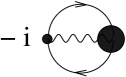
Figure 2: Ghost/fermion part of $\Gamma_{2}^{0}$.

The equivalence of the 4PI effective action to three-loop order with the 3PI and $n$PI effective actions for $n\geq 5$ in the absence of sources follows along the lines of Sec. 2.2. As a consequence, to three-loop order the $n$PI effective action does not depend on higher vertices $V_{5}$, $V_{6}$, …$V_{n}$. In particular with vanishing sources the four-vertex is given by the classical one:

$$\frac{\delta\Gamma^{\rm(3loop)}[D,G,V_{3},V_{3}^{\rm(gh)},V_{4}]}{\delta V_{4}}=\frac{\delta\Gamma^{\rm(3loop)}_{2}[D,G,V_{3},V_{3}^{\rm(gh)},V_{4}]}{\delta V_{4}}=0\,\,\Rightarrow\,\,V_{4}=V_{04}.$$ (3.74)

If one plugs this into (3.72) and (3.73) one obtains the three-loop 3PI effective action, $\Gamma^{\rm(3loop)}[\phi,D,V_{3},V_{3}^{\rm(gh)}]$. Similarly, to two-loop order one has

$$\frac{\delta\Gamma^{\rm(2loop)}[D,G,V_{3},V_{3}^{\rm(gh)}]}{\delta V_{3}} \!=\! \frac{\delta\Gamma^{\rm(2loop)}_{2}[D,G,V_{3},V_{3}^{\rm(gh)}]}{\delta V_{3}}=0\,\,\Rightarrow\,\,V_{3}=V_{03}\,,$$

$$\frac{\delta\Gamma^{\rm(2loop)}[D,G,V_{3},V_{3}^{\rm(gh)}]}{\delta V_{3}^{\rm(gh)}} \!=\! \frac{\delta\Gamma^{\rm(2loop)}_{2}[D,G,V_{3},V_{3}^{\rm(gh)}]}{\delta V_{3}^{\rm(gh)}}=0\,\,\Rightarrow\,\,V_{3}^{\rm(gh)}=V_{03}^{\rm(gh)}\,,$$

and equivalently for the fermion vertex $V_{3}^{\rm(f)}$. To this order, therefore, the combinatorial factors of the two-loop diagrams of Fig. 1 and 3 for the gauge part, as well as of Fig. 2 and 4 for the ghost/fermion part, combine to give the result (3.69) to two-loop order for the 2PI effective action.

Figure 3: The figure shows together with Fig. 4 the diagrammatic representation of $\Gamma_{2}^{\rm int}[D,G,V_{3},V_{3}^{\rm(gh)},V_{4}]$ to three-loop order as given in Eq. (3.73). For the gauge theory with fermions, to this order there is in addition the same contribution as in Fig. 4 with the unwiggled propagator lines representing the fermion propagator $\Delta$ and the ghost vertex replaced by the corresponding fermion vertex $V_{3}^{\rm(f)}$. This functional contains no explicit dependence on the classical vertices independent of the order of approximation.

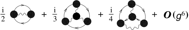
Figure 4: Ghost/fermion part of $\Gamma_{2}^{\rm int}$ to three-loop order.

4 Equations of motion

In the last section we have seen that to two-loop order the proper vertices of the $n$PI effective action correspond to the classical ones. Accordingly, at this order the only non-trivial equations of motion in the absence of background fields are those for the two-point functions:

$$\frac{\delta\Gamma}{\delta D}=0\,,\quad\,\frac{\delta\Gamma}{\delta G}=0\,,\quad\,\frac{\delta\Gamma}{\delta\Delta}=0\,,$$ (4.75)

for vanishing sources. Applied to an $n$PI effective action ($n>1$), as e.g. (3.71), one finds for the gauge field propagator:

$$D^{-1}=D^{-1}_{0}-\Pi\,,$$ (4.76)

where the proper self-energy is given by

$$\Pi=2i\,\frac{\delta\Gamma_{2}}{\delta D}\,.$$ (4.77)

The ghost propagator and self-energy are

$$G^{-1}=G^{-1}_{0}-\Sigma\quad,\quad\Sigma=-i\frac{\delta\Gamma_{2}}{\delta G}\,,$$ (4.78)

and equivalently for the fermion propagator $\Delta$. The self-energies to this order are shown in diagrammatic form in Fig. 5. In contrast, for the three-loop effective action the three-vertices get dressed and the stationarity conditions,

$$\frac{\delta\Gamma}{\delta V_{3}}=0\,,\quad\,\frac{\delta\Gamma}{\delta V_{3}^{\rm(gh)}}=0\,,\quad\,\frac{\delta\Gamma}{\delta V_{3}^{\rm(f)}}=0\,,$$ (4.79)

applied to (3.71)–(3.73) lead to the equations shown in Fig. 7. Here the diagrammatic form of the contributions is always the same for the ghost and for the fermion propagators or vertices. We therefore only give the expressions for the gauge-ghost system. If fermions are present, the respective diagrams have to be added in a straightforward way.

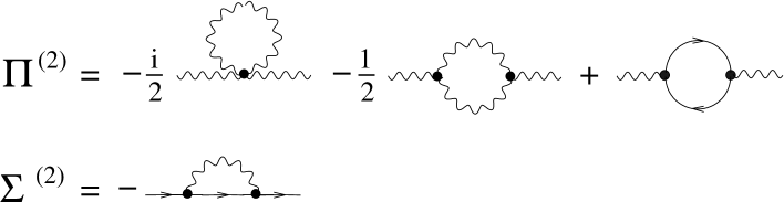
Figure 5: The self-energy for the gauge field ($\Pi$) and the ghost/fermion ($\Sigma$) propagators as obtained from the self-consistently complete two-loop approximation of the effective action. Note that at this order all vertices correspond to the classical ones.

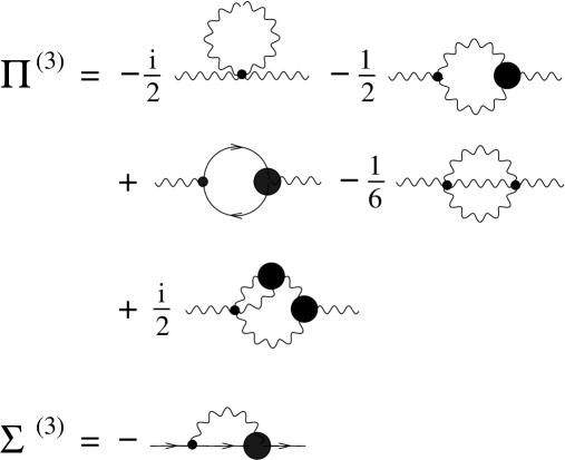
Figure 6: The self-energy for the gauge field ($\Pi$) and the ghost/fermion ($\Sigma$) propagators as obtained from the self-consistently complete three-loop approximation of the effective action. (Cf. Fig. 7 for the vertices.)

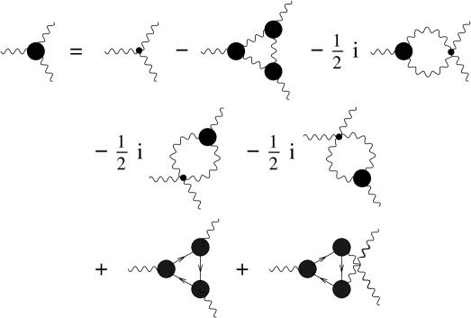
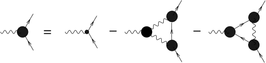
Figure 7: The gauge field three-vertex as well as the ghost (fermion) vertex as obtained from the self-consistently complete three-loop approximation of the effective action. Note that apart from the isolated classical three-vertex, all vertices in the equations correspond to dressed ones since at this order the four-vertex equals the classical vertex.

The respective self-energies to this order are displayed in Fig. 6. It should be emphasized that their relatively simple form is a consequence of the equations for the proper vertices, Fig. 7. To see this we consider first the many terms generated by the functional derivative of (3.72) and (3.73) with respect to the gauge field propagator:

$$\Pi^{(3)}\,\equiv\,2i\frac{\delta\Gamma_{2}^{\rm(3loop)}}{\delta D} \!=\! -\frac{i}{2}\,\begin{minipage}{34.14322pt} \psfig{width=34.14322pt} \end{minipage}-\begin{minipage}{39.83368pt} \psfig{width=39.83368pt} \end{minipage}+\frac{1}{2}\,\begin{minipage}{39.83368pt} \psfig{width=39.83368pt} \end{minipage}+2\,\begin{minipage}{39.83368pt} \psfig{width=39.83368pt} \end{minipage}$$

$$-\,\begin{minipage}{39.83368pt} \psfig{width=39.83368pt} \end{minipage}-\frac{1}{3}\,\begin{minipage}{39.83368pt} \psfig{width=39.83368pt} \end{minipage}+\frac{1}{6}\,\begin{minipage}{39.83368pt} \psfig{width=39.83368pt} \end{minipage}+i\,\begin{minipage}{39.83368pt} \psfig{width=39.83368pt} \end{minipage}$$

$$+\frac{i}{4}\,\begin{minipage}{48.36958pt} \psfig{width=48.36958pt} \end{minipage}+\frac{1}{2}\,\begin{minipage}{45.52458pt} \psfig{width=45.52458pt} \end{minipage}-2\,\begin{minipage}{45.52458pt} \psfig{width=45.52458pt} \end{minipage}-\,\begin{minipage}{45.52458pt} \psfig{width=45.52458pt} \end{minipage}\,.$$

The short form for the self-energy of Fig. 6 is obtained through cancellations by replacing in the above expression

$$\frac{1}{2}\,\begin{minipage}{39.83368pt} \psfig{width=39.83368pt} \end{minipage} \!=\! \frac{1}{2}\,\begin{minipage}{39.83368pt} \psfig{width=39.83368pt} \end{minipage}-\frac{1}{2}\,\begin{minipage}{45.52458pt} \psfig{width=45.52458pt} \end{minipage}-\frac{i}{4}\,\begin{minipage}{45.52458pt} \psfig{width=45.52458pt} \end{minipage}$$ (4.81)

$$-\frac{i}{2}\,\begin{minipage}{45.52458pt} \psfig{width=45.52458pt} \end{minipage}+\,\begin{minipage}{45.52458pt} \psfig{width=45.52458pt} \end{minipage}$$

as well as

$$-\,\begin{minipage}{39.83368pt} \psfig{width=39.83368pt} \end{minipage} \!=\! -\,\begin{minipage}{39.83368pt} \psfig{width=39.83368pt} \end{minipage}+\,\begin{minipage}{45.52458pt} \psfig{width=45.52458pt} \end{minipage}+\,\begin{minipage}{45.52458pt} \psfig{width=45.52458pt} \end{minipage}\,.$$ (4.82)

The latter equations follow from inserting the expressions for the dressed vertices of Fig. 7. Noting in addition that the proper four-vertex to this order corresponds to the classical one (cf. (3.74)) leads to the result. Along the very same lines a similar cancellation yields the compact form of the ghost/fermion self-energy displayed in Fig. 6.

4.1 Comparison with Schwinger-Dyson equations

The equations of motions of the last section are self-consistently complete to two-loop/three-loop order of the $n$PI effective action for arbitrarily large $n$. We now compare them with conventional Schwinger-Dyson (SD) equations, which represent identities between $n$-point functions. Clearly, without approximations the equations of motion obtained from an exact $n$PI effective action and the exact (SD) equations have to agree since one can always map identities onto each other. However, in general this is no longer the case for a given order in the loop expansion of the $n$PI effective action.

By construction each diagram in a SD equation contains at least one classical vertex [33]. In general, this is not the case for equations obtained from the $n$PI effective action: The loop contributions of $\Gamma_{2}^{\rm int}$ in Eq. (3.73) or Figs. 3–4 are solely expressed in terms of full vertices. However, to a given loop-order cancellations can occur for those diagrams in the equations of motion which do not contain a classical vertex. For the three-loop effective action result this has been demonstrated in Sec. 4 for the two-point functions. Indeed, the equations for the two-point functions shown in Fig. 6 correspond to the SD equations, if one takes into account that to the considered order the four-vertex is trivial and given by the classical one (cf. 3.74). However, such a correspondence is not true for the proper three-vertex to that order.

As an example, we show in Fig. 8 the standard (SD) equation for the proper three-vertex, where we neglect for a moment the additional diagrams coming from ghost/fermion degrees of freedom (cf. e.g. [37]). One finds that a naive neglection of the two-loop contributions of that equation would not lead to the effective action result for the three-vertex shown in Fig. 7. Of course, the straightforward one-loop truncation of the SD equation would not even respect the property of $V_{3}$ being completely symmetric in its space-time and group labels. This is the well-known problem of loop-expansions of SD equations, where one encounters the ambiguity of whether classical or dressed vertices should be employed at a given truncation order.

Figure 8: Standard Schwinger-Dyson equation for the proper three-vertex $V_{3}$. We have not displayed additional diagrams involving ghost or fermion vertices for brevity. We show it for comparison with the three-loop effective action result displayed in Fig. 7. One observes that a naive truncation of the Schwinger-Dyson equation at the one-loop level does not agree with the latter, since the second and third diagram contain a classical three-vertex instead of a dressed one as in Fig. 7. (Note that the four-vertex equals the classical one at this order in the self-consistently complete loop expansion.)

We emphasize that these problems are absent using effective action techniques. The fact that all equations of motion are obtained from the same approximation of the effective action puts stringent conditions on their form. More precisely, a self-consistently complete approximation has the property that the order of differentiation of, say, $\Gamma[D,V]$ with respect to the propagator $D$ or the vertex $V$ does not affect the equations of motion. Consider for instance:

$$\frac{\delta\Gamma[D,V=V(D)]}{\delta D}=\frac{\delta\Gamma}{\delta D}\Big{|}_{V}+\frac{\delta\Gamma}{\delta V}\Big{|}_{D}\,\frac{\delta V}{\delta D}\,.$$ (4.83)

If $V=V(D)$ is the result of the stationary condition $\delta\Gamma/\delta V=0$ then the above corresponds to the correct stationarity condition for the propagator for fixed $V$: $\delta\Gamma/\delta D=0$. In contrast, with some ansatz $V=f(D)$ that does not fulfill the stationarity condition of the effective action, the equation of motion for the propagator would receive additional corrections $\sim\delta V/\delta D$. In particular, it would be inconsistent to use the equation of motion for the propagator $\delta\Gamma/\delta D=0$ (cf. e.g. Fig. 6 which corresponds to the SD equation result) but not the equation $\delta\Gamma/\delta V=0$ for the vertex (cf. Fig. 7).

In turn, one can conclude that a wide class of employed truncations of exact SD equations cannot be obtained from the $n$PI effective action: this concerns those approximations which use the exact SD equation for the propagator but make an ansatz for the vertices that differs from the one displayed in Fig. 7. The differences are, however, typically higher order in the perturbative coupling expansion and there may be many cases, in particular in vacuum or thermal equilibrium, where some ansatz for the vertices is a very efficient way to proceed. Out of equilibrium however, as mentioned above, the “conserving” property of the effective action approximations can have important consequences, since the effective loss of initial conditions and the presence of basic constants of motion such as energy conservation is crucial.

5 Nonequilibrium evolution equations

The above equations of motion have the form of self-consistent or “gap” equations, as in (4.76) or (4.78), which is very suitable for vacuum or thermal equilibrium problems. In this case the time integrations displayed in Sec. 3 run along the real axis ($\int_{x}\equiv\int_{-\infty}^{\infty}{\rm d}^{d+1}x$) or along the imaginary time-axis ($\int_{x}\equiv\int_{0}^{-i\beta}{\rm d}x^{0}\int{\rm d}{\bf x}$) up to the inverse temperature $\beta$, respectively [38]. For nonequilibrium time-evolution problems it is useful to rewrite the equations in a standard way such that they are suitable for initial-value problems. The time integration in this case starts at some initial time and involves a closed path $\mathcal{C}$ along the real axis ($\int_{x}\equiv\int_{\mathcal{C}}{\rm d}x^{0}\int{\rm d}{\bf x}$) [39].

Up to $\mathcal{O}(g^{6})$ corrections in the self-consistently complete expansion of the effective action, the four-vertex parametrizing the diagrams of Figs. 6–7 corresponds to the classical vertex. At this order of approximation there is, therefore, no distinction between the coupling expansion of the 3PI and 4PI effective action. To discuss the relevant differences between the 2PI and 3PI expansions for time evolution problems, we will use the language of QED for simplicity, where no four-vertex appears. However, the evolution equations of this section can be straightforwardly transcribed to the nonabelian case by taking into account in addition to the equation for the gauge–fermion three-vertex those for the gauge–ghost and gauge three-vertex (cf. Fig. 7). In the following the effective action is a functional of the gauge field propagator $D_{\mu\nu}(x,y)$, the fermion propagator $\Delta(x,y)$ and the gauge-fermion vertex $V_{3\,\mu}^{\rm(f)}(x,y;z)$, where we suppress Dirac indices and we will write $V_{3}^{\rm(f)}\equiv V$. According to Eqs. (3.71)—(3.73) one has in this case

$$\Gamma_{2}[D,\Delta,V]=\Gamma_{2}^{0}[D,\Delta,V]+\Gamma_{2}^{\rm int}[D,\Delta,V]\,,$$ (5.84)

with

$$\Gamma_{2}^{0}=-ig^{2}\int_{xyzu}\hbox{tr}\left[\gamma_{\mu}\Delta(x,y)V_{\nu}(y,z;u)\Delta(z,x)D^{\mu\nu}(x,u)\right]\,,$$ (5.85)

where the trace acts in Dirac space. For the given order of approximation there are two distinct contributions to $\Gamma_{2}^{\rm int}$:

$$\Gamma_{2}^{\rm int} = \Gamma_{2}^{(a)}+\Gamma_{2}^{(b)}+\mathcal{O}\left(g^{6}\right)\,,$$ (5.86)

$$\Gamma_{2}^{(a)} = \frac{i}{2}g^{2}\int_{xyzuvw}\hbox{tr}\left[V_{\mu}(x,y;z)\Delta(y,u)V_{\nu}(u,v;w)\Delta(v,x)D^{\mu\nu}(z,w)\right]\,,$$

$$\Gamma_{2}^{(b)} = \frac{i}{4}g^{4}\int_{xyzuvwx^{\prime}y^{\prime}z^{\prime}u^{\prime}v^{\prime}w^{\prime}}\hbox{tr}\left[V_{\mu}(x,y;z)\Delta(y,u)V_{\nu}(u,v;w)\Delta(v,x^{\prime})\right.$$

$$\left.V_{\rho}(x^{\prime},y^{\prime};z^{\prime})\Delta(y^{\prime},u^{\prime})V_{\sigma}(u^{\prime},v^{\prime};w^{\prime})\Delta(v^{\prime},x)D^{\mu\rho}(z,z^{\prime})D^{\nu\sigma}(w,w^{\prime})\right]\,.$$

The equations of motions for the propagators and vertex are obtained from the stationarity conditions (4.75) and (4.79) for the effective action. To convert (4.76) for the photon propagator into an equation which is more suitable for initial value problems, we convolute with $D$ from the right and obtain for the considered case of vanishing ‘background’ fields, e.g. for covariant gauges:

$$\left[{g^{\mu}}_{\gamma}\square-(1-\xi^{-1})\partial^{\mu}\partial_{\gamma}\right]_{x}D^{\gamma\nu}(x,y)-i\int_{z}{\Pi^{\mu}}_{\gamma}(x,z)D^{\gamma\nu}(z,y)$$

$$=ig^{\mu\nu}\delta_{\mathcal{C}}(x-y)\,.$$ (5.87)

Similarly, the corresponding equation of (4.78) yields the evolution equation for the fermion propagator:

$$i\partial_{x}\!\!\!\!\!/\,\,\Delta(x,y)-i\int_{z}\Sigma(x,z)\Delta(z,y)=i\delta_{\mathcal{C}}(x-y)\,.$$ (5.88)

Using the results of Sec. 4 the self-energies are

$$\Sigma(x,y) = -g^{2}\int_{z^{\prime}z^{\prime\prime}}D_{\mu\nu}(z^{\prime},y)V^{\mu}(x,z^{\prime\prime};z^{\prime})\Delta(z^{\prime\prime},y)\gamma^{\nu}\,,$$ (5.89)

$$\Pi^{\mu\nu}(x,y) = g^{2}\int_{z^{\prime}z^{\prime\prime}}\hbox{tr}\,\gamma^{\mu}\Delta(x,z^{\prime})V^{\nu}(z^{\prime},z^{\prime\prime};y)\Delta(z^{\prime\prime},x)\,.$$ (5.90)

Note that the form of the self-energies is exact for known three-vertex. To see this within the current framework, we note that the self-energies can be expressed in terms of $\Gamma_{2}^{0}$ only. The latter receives no further corrections at higher order in the expansion (cf. Sec. 3.2), and thus the expression is exactly known: With

$$\int_{z}\Sigma(x,z)\Delta(z,y)=-i\int_{z}\left(\frac{\delta\Gamma_{2}^{0}}{\delta\Delta(z,x)}+\frac{\delta\Gamma_{2}^{\rm int}}{\delta\Delta(z,x)}\right)\Delta(z,y)\,,$$ (5.91)

and since $\Gamma_{2}^{\rm int}$ is only a functional of $V\Delta D^{1/2}$ (cf. Sec. 3.2) one can use the identity

$$\int_{z}\frac{\delta\Gamma_{2}^{\rm int}}{\delta\Delta(z,x)}\Delta(z,y) = \int_{zz^{\prime}}V_{\mu}(x,z;z^{\prime})\frac{\delta\Gamma_{2}^{\rm int}}{V_{\mu}(y,z;z^{\prime})}$$ (5.92)

$$= -\int_{zz^{\prime}}V_{\mu}(x,z;z^{\prime})\frac{\delta\Gamma_{2}^{0}}{V_{\mu}(y,z;z^{\prime})}$$

to express everything in terms of the known $\Gamma_{2}^{0}$. The last equality in (5.92) uses that $\delta(\Gamma_{2}^{0}+\Gamma_{2}^{\rm int})/\delta\Delta=0$. A similar discussion can be done for the photon self-energy. As a consequence, all approximations are encoded in the equation for the vertex, which is obtained from (5.86) as:

$$V^{\mu}(x,y;z) = V_{0}^{\mu}(x,y;z)-g^{2}\int_{vwx^{\prime}y^{\prime}u^{\prime}w^{\prime}}V_{\nu}(x,v;w)\Delta(v,x^{\prime})V^{\mu}(x^{\prime},y^{\prime};z)$$ (5.93)

$$\Delta(y^{\prime},u^{\prime})V_{\sigma}(u^{\prime},y;w^{\prime})D^{\sigma\nu}(w^{\prime},w)+\mathcal{O}\left(g^{4}\right)\,,$$

where

$$V_{0}^{\mu}(x,y;z)=\gamma^{\mu}\delta(x-z)\delta(z-y)\,.$$ (5.94)

For the self-consistently complete two-loop approximation the self-energies are given by

$$\Sigma(x,y) = -g^{2}D_{\mu\nu}(x,y)\gamma^{\mu}\Delta(x,y)\gamma^{\nu}+\mathcal{O}\left(g^{4}\right)\,,$$ (5.95)

$$\Pi^{\mu\nu}(x,y) = g^{2}\,\hbox{tr}\,\gamma^{\mu}\Delta(x,y)\gamma^{\nu}\Delta(y,x)+\mathcal{O}\left(g^{4}\right)\,.$$ (5.96)

5.1 Spectral and statistical correlation functions

We decompose the two-point functions into ‘spectral’ and ‘statistical components’ by writing [7, 4]

$$D^{\mu\nu}(x,y) = F_{D}(x,y)^{\mu\nu}-\frac{i}{2}\rho_{D}(x,y)^{\mu\nu}\,{\rm sign}(x^{0}-y^{0})\,.$$ (5.97)

Here $\rho_{D}$ corresponds to the spectral function and $F_{D}$ is the so-called statistical two-point function. Equivalently, the decomposition identity of the fermion two-point function into spectral and statistical components reads [9]

$$\Delta(x,y) = F_{\Delta}(x,y)-\frac{i}{2}\rho_{\Delta}(x,y)\,{\rm sign}(x^{0}-y^{0})\,.$$ (5.98)

The same decomposition can be done for the corresponding self-energies:

$$\Pi^{\mu\nu}(x,y) = \Pi_{(F)}(x,y)^{\mu\nu}-\frac{i}{2}\Pi_{(\rho)}(x,y)^{\mu\nu}\,{\rm sign}(x^{0}-y^{0})\,,$$ (5.99)

$$\Sigma(x,y) = \Sigma_{(F)}(x,y)-\frac{i}{2}\Sigma_{(\rho)}(x,y)\,{\rm sign}(x^{0}-y^{0})\,.$$ (5.100)

Since the above decomposition for the propagators and self-energies makes the time-ordering explicit, we can evaluate the RHS of (5.87) along the time contour [4], and one finds the evolution equations (cf. also [16]):

$$\left[{g^{\mu}}_{\gamma}\square-(1-\xi^{-1})\partial^{\mu}\partial_{\gamma}\right]_{x}\rho_{D}(x,y)^{\gamma\nu} = \int_{y^{0}}^{x^{0}}{\rm d}z\,\Pi_{(\rho)}(x,z)^{\mu\gamma}\rho_{D}{(z,y)_{\gamma}}^{\nu}\,\,\,,$$

$$\left[{g^{\mu}}_{\gamma}\square-(1-\xi^{-1})\partial^{\mu}\partial_{\gamma}\right]_{x}F_{D}(x,y)^{\gamma\nu} = \int_{t_{0}}^{x^{0}}{\rm d}z\,\Pi_{(\rho)}(x,z)^{\mu\gamma}F_{D}{(z,y)_{\gamma}}^{\nu}$$

$$- \int_{t_{0}}^{y^{0}}{\rm d}z\,\Pi_{(F)}(x,z)^{\mu\gamma}\rho_{D}{(z,y)_{\gamma}}^{\nu}\,\,\,,$$

where we used the abbreviated notation $\int_{t_{1}}^{t_{2}}{\rm d}z\equiv\int_{t_{1}}^{t_{2}}{\rm d}z^{0}\int_{-\infty}^{\infty}{\rm d}\bf{z}$. The equations of motion for the fermion spectral and statistical correlators are obtained from (5.88) [9]:

$$i{\partial\,\!\!\!\!/\,}_{\!x}\rho_{\Delta}(x,y) = \int_{y^{0}}^{x^{0}}{\rm d}z\,\Sigma_{(\rho)}(x,z)\rho_{\Delta}(z,y)\,,$$ (5.103)

$$i{\partial\,\!\!\!\!/\,}_{\!x}F_{\Delta}(x,y) = \int_{0}^{x^{0}}{\rm d}z\,\Sigma_{(\rho)}(x,z)F_{\Delta}(z,y)-\int_{0}^{y^{0}}{\rm d}z\,\Sigma_{(F)}(x,z)\rho_{\Delta}(z,y)\,.$$

For known self-energies the equations (LABEL:eq:rho)–(LABEL:eq:Fexact) are exact. One observes that the form of their RHS is independent of whether it describes a boson or a fermion correlator.

A similar discussion as for the two-point functions can also be done for the higher correlation functions. For the three-vertex we write

$$V^{\mu}(x,y;z)=V_{0}^{\mu}(x,y;z)+\bar{V}^{\mu}(x,y;z)\,.$$ (5.105)

and the corresponding decomposition into spectral and statistical components reads

$$\bar{V}^{\mu}(x,y;z)=$$

$$U_{(F)}(x,y;z)^{\mu}\,{\rm sign}(y^{0}-x^{0})\,{\rm sign}(z^{0}-x^{0})-\frac{i}{2}U_{(\rho)}(x,y;z)^{\mu}\,{\rm sign}(y^{0}-z^{0})$$

$$\!+\!\! V_{(F)}(x,y;z)^{\mu}\,{\rm sign}(x^{0}-z^{0})\,{\rm sign}(y^{0}-z^{0})-\frac{i}{2}V_{(\rho)}(x,y;z)^{\mu}\,{\rm sign}(x^{0}-y^{0})$$

$$\!+\!\! W_{(F)}(x,y;z)^{\mu}\,{\rm sign}(z^{0}-y^{0})\,{\rm sign}(x^{0}-y^{0})-\frac{i}{2}W_{(\rho)}(x,y;z)^{\mu}\,{\rm sign}(z^{0}-x^{0}).$$

This will be discussed further in the appendix.

6 Kinetic theory and the LPM effect

As an application we will consider the above equations in a standard “on-shell” limit which is typically employed in the literature to derive kinetic equations for effective particle number densities [16]. We will see that since the lowest order contribution to the kinetic equation is of ${\mathcal{O}}(g^{4})$, the 3PI effective action provides a self-consistently complete starting point for its description. To this order the effective action resums in particular all diagrams enhanced by the Landau Pomeranchuk Migdal effect [30], which has been extensively discussed in recent literature in the context of transport coefficients for gauge theories [29].

6.1 “On-shell” limits

The evolution equations (LABEL:eq:rho)–(LABEL:eq:Fexact) to order $g^{2}$ and higher contain so-called “off-shell” and “memory” effects due to their time integrals on the RHS. To simplify the description one may consider a number of additional assumptions which finally lead to effective kinetic or Boltzmann-type descriptions for on-shell particle number distributions. Much of this discussion is standard and can be found e.g. summarized in Ref. [16], and we will only repeat what is necessary for our purposes. The derivation of kinetic equations for the two-point functions $F^{\mu\nu}(x,y)$ and $\rho^{\mu\nu}(x,y)$ of Sec. 5.1 can be based on (i) the restriction that the initial condition for the time evolution problem is specified in the remote past, i.e. $t_{0}\to-\infty$, (ii) a derivative expansion in the center variable $X=(x+y)/2$, and (iii) a ‘quasiparticle’ picture. To make contact with the literature we will adopt this standard procedure in the following and discuss limitations in Sec. 6.2.

For the sake of simplicity (not required), we consider the Feynman gauge $\xi=1$ in the following. We will also consider a chirally symmetric theory, i.e. no vacuum fermion mass, along with parity and $CP$ invariance. Therefore, the system is charge neutral and, in particular, the most general fermion two-point functions can be written in terms of vector components only [9]: $F_{\Delta}(x,y)=\gamma_{\mu}F_{\Delta}(x,y)^{\mu}$, $\rho_{\Delta}(x,y)=\gamma_{\mu}\rho_{\Delta}(x,y)^{\mu}$, with hermiticity properties $F_{\Delta}(x,y)^{\mu}=[F_{\Delta}(y,x)^{\mu}]^{*}$, $\rho_{\Delta}(x,y)^{\mu}=-[\rho_{\Delta}(y,x)^{\mu}]^{*}$. For the gauge fields the respective properties of the statistical and spectral correlators read $F_{D}(x,y)^{\mu\nu}=[F_{D}(y,x)^{\nu\mu}]^{*}$, $\rho_{D}(x,y)^{\mu\nu}=-[\rho_{D}(y,x)^{\nu\mu}]^{*}$.

In order to Fourier transform with respect to the relative coordinate $s^{\mu}=x^{\mu}-y^{\mu}$, we write

$$\tilde{F}_{D}\left(X,k\right)^{\mu\nu} = \int{\rm d}^{4}{s}\;e^{iks}F_{D}\left(X+\frac{s}{2},X-\frac{s}{2}\right)^{\mu\nu}\;,$$ (6.107)

$$\tilde{\varrho}_{D}\left(X,k\right)^{\mu\nu} = -i\int{\rm d}^{4}{s}\;e^{iks}\rho_{D}\left(X+\frac{s}{2},X-\frac{s}{2}\right)^{\mu\nu}\;,$$ (6.108)

and equivalently for the fermion statistical and spectral function, $\tilde{F}_{\Delta}(X,k)$ and $\tilde{\varrho}_{\Delta}(X,k)$. Here we have introduced a factor $-i$ in the definition of the spectral function transform for convenience. For the Fourier transformed quantities we note the following hermiticity properties, for the gauge fields: $[\tilde{F}_{D}(X,k)^{\mu\nu}]^{*}=\tilde{F}_{D}(X,k)^{\nu\mu}\,\,,\,\,[\tilde{\varrho}_{D}(X,k)^{\mu\nu}]^{*}=\tilde{\varrho}_{D}(X,k)^{\nu\mu}$, and for the vector components of the fermion fields: $[\tilde{F}_{\Delta}(X,k)^{\mu}]^{*}=\tilde{F}_{\Delta}(X,k)^{\mu}\,\,,\,\,[\tilde{\varrho}_{\Delta}(X,k)^{\mu}]^{*}=\tilde{\varrho}_{\Delta}(X,k)^{\mu}$. After sending $t_{0}\to-\infty$ the derivative expansion can be efficiently applied to the exact Eqs. (LABEL:eq:rho)—(LABEL:eq:Fexact). Here one considers the difference of (LABEL:eq:rho) and the one with interchanged coordinates $x$ and $y$, and equivalently for the other equations. We use

$$\int\!{\rm d}^{4}{s}\;e^{iks}\int\!{\rm d}^{4}{z}f(x,z)g(z,y) \!=\! \tilde{f}(X,k)\tilde{g}(X,k)+\ldots\,\,$$ (6.109)

$$\int\!{\rm d}^{4}{s}\;e^{iks}\int\!{\rm d}^{4}{z}\int\!{\rm d}^{4}{z^{\prime}}f(x,z)g(z,z^{\prime})h(z^{\prime},y) \!=\! \tilde{f}(X,k)\tilde{g}(X,k)\tilde{h}(X,k)+\ldots$$

where the dots indicate derivative terms, which will be neglected. E.g. the first derivative corrections to (6.109) can be written as a Poisson bracket [16], which is in particular important if ‘finite-width’ effects of the spectral function are taken into account. However, a typical quasiparticle picture which employs a free-field or ‘zero-width’ form of the spectral function is consistent with neglecting derivative terms in the scattering part. We also note that the quasiparticle/free-field form of the two-point functions implies

$$F_{D}(X,k)^{\mu\nu}\to-g^{\mu\nu}F_{D}(X,k)\quad,\quad\rho_{D}(X,k)^{\mu\nu}\to-g^{\mu\nu}\rho_{D}(X,k)\,.$$ (6.110)

At this point the only use of the above replacement is that all Lorentz contractions can be done. This doesn’t affect the derivative expansion but keeps the notation simple. Similar to Eq. (6.108), we define the Lorentz contracted self-energies:

$$-4\tilde{\Pi}_{(F)}(X,k) \equiv \int{\rm d}^{4}{s}\;e^{iks}\Pi_{(F)}{\left(X+\frac{s}{2},X-\frac{s}{2}\right)^{\mu}}_{\mu}\,,$$ (6.111)

$$-4\tilde{\Pi}_{(\varrho)}(X,k) \equiv -i\int{\rm d}^{4}{s}\;e^{iks}\Pi_{(\rho)}{\left(X+\frac{s}{2},X-\frac{s}{2}\right)^{\mu}}_{\mu}\,.$$ (6.112)

Without further assumptions, i.e. using the above notation and applying the approximation (6.109) and (6.110) to the exact evolution equations one has (cf. also [40])

$$2\,k^{\mu}\frac{\partial}{\partial X^{\mu}}\tilde{F}_{D}(X,k) = \tilde{\Pi}_{(\varrho)}(X,k)\,\tilde{F}_{D}(X,k)-\tilde{\Pi}_{(F)}(X,k)\,\tilde{\varrho}_{D}(X,k)\,,\qquad$$ (6.113)

$$2\,k^{\mu}\frac{\partial}{\partial X^{\mu}}\tilde{\varrho}_{D}(X,k) = 0\,.$$ (6.114)

One observes that the equations (6.113) and (6.114) have a structure reminiscent of that for the exact equations for vanishing ‘background’ fields, (LABEL:eq:rho) and (LABEL:eq:F), evaluated at equal times $x^{0}=y^{0}$. However, one should keep in mind that (6.113) and (6.114) are, in particular, only valid for initial conditions specified in the remote past and neglecting gradients in the collision part.

From (6.114) one observes that in this approximation the spectral function receives no contribution from scattering described by the RHS of the exact equation (LABEL:eq:rho). As a consequence, the spectral function obeys the free-field equations of motion. In particular, $\rho_{D}^{\mu\nu}(x,y)$ have to fulfill the equal-time commutation relations $[\rho_{D}^{\mu\nu}(x,y)]_{x^{0}=y^{0}}=0$ and $[\partial_{x^{0}}\rho_{D}^{\mu\nu}(x,y)]_{x^{0}=y^{0}}=-g^{\mu\nu}\delta({\bf x}-{\bf y})$ in Feynman gauge. The Wigner transformed free-field solution solving (6.114) then reads $\tilde{\varrho}_{D}(X,k)=\tilde{\varrho}_{D}(k)=2\pi\,{\rm sign}(k^{0})\,\delta(k^{2})$. A very similar discussion can be done as well for the evolution equations (5.103) and (LABEL:eq:Fexact) for fermions, which is massless due to chiral symmetry as stated above. Again, in lowest order in the derivative expansion the fermion spectral function obeys the free-field equations of motion and one has $\tilde{\varrho}_{\Delta}(X,k)=\tilde{\varrho}_{\Delta}(k)=2\pi k\,\!\!\!\!/\,\,{\rm sign}(k^{0})\,\delta(k^{2})$.

6.1.1 Vanishing of the ${\mathcal{O}}(g^{2})$ on-shell contributions

Assuming a “generalized fluctuation-dissipation relation” or so-called Kadanoff-Baym ansatz [41]:

$$\tilde{F}_{D}(X,k) = \left[\frac{1}{2}+n_{D}(X,k)\right]\tilde{\varrho}_{D}(X,k)\,,$$

$$\tilde{F}_{\Delta}(X,k) = \left[\frac{1}{2}-n_{\Delta}(X,k)\right]\tilde{\varrho}_{\Delta}(X,k)\,,$$ (6.115)

one may extract the kinetic equations for the effective photon and fermion particle numbers $n_{D}$ and $n_{\Delta}$, respectively. Considering spatially homogeneous, isotropic systems for simplicity, we define the on-shell quasiparticle numbers ($t\equiv X^{0}$)

$$n_{D}(t,{\bf k})\equiv n_{D}(t,k)|_{k^{0}=|{\bf k}|}\quad,\quad n_{\Delta}(t,{\bf k})\equiv n_{\Delta}(t,k)|_{k^{0}=|{\bf k}|}$$ (6.116)

and look for the evolution equation for $n_{D}(t,{\bf k})=n_{D}(t,|{\bf k}|)$. Here it is useful to note the symmetry properties

$$\tilde{F}_{D}(t,-k) = \tilde{F}_{D}(t,k)\,\,,\,\,\tilde{\varrho}_{D}(t,-k)=-\tilde{\varrho}_{D}(t,k)\,,$$

$$\tilde{F}_{\Delta}(t,-k)^{\mu} = -\tilde{F}_{\Delta}(t,k)^{\mu}\,\,,\,\,\tilde{\varrho}_{\Delta}(t,-k)^{\mu}=\tilde{\varrho}_{\Delta}(t,k)^{\mu}\,.$$ (6.117)

Applied to the quasiparticle ansatz (6.115) these imply

$$n_{D}(t,-k)=-\left[n_{D}(t,k)+1\right]\,\,\,,\,\,\,n_{\Delta}(t,-k)=-\left[n_{\Delta}(t,k)-1\right]$$ (6.118)

This is employed to rewrite terms with negative values of $k^{0}$. To order $g^{2}$ the self-energies read (cf. Eq. (5.96)):

$$\tilde{\Pi}_{(F)}(X,k) = 2g^{2}\int\frac{{\rm d}^{4}p}{(2\pi)^{4}}\Big{[}\tilde{F}_{\Delta}(X,k+p)^{\mu}\tilde{F}_{\Delta}(X,p)_{\mu}$$

$$-\frac{1}{4}\tilde{\varrho}_{\Delta}(X,k+p)^{\mu}\tilde{\varrho}_{\Delta}(X,p)_{\mu}\Big{]}\,,$$

$$\tilde{\Pi}_{(\varrho)}(X,k) = 2g^{2}\int\frac{{\rm d}^{4}p}{(2\pi)^{4}}\Big{[}\tilde{F}_{\Delta}(X,k+p)^{\mu}\tilde{\varrho}_{\Delta}(X,p)_{\mu}$$ (6.119)

$$-\tilde{\varrho}_{\Delta}(X,k+p)^{\mu}\tilde{F}_{\Delta}(X,p)_{\mu}\Big{]}\,.$$

From the equations (6.113) and (6.115) one finds at this order: (${\bf q}\equiv{\bf k}-{\bf p}$)

$$\partial_{t}n_{D}(t,|{\bf k}|)=g^{2}k^{2}\int\frac{{\rm d}^{3}p}{(2\pi)^{3}}\,\frac{1}{2|{\bf k}|2|{\bf p}|2|{\bf q}|}\Bigg{\{}$$ (6.120)

$$\Big{(}n_{\Delta}(t,|{\bf p}|)\,n_{\Delta}(t,|{\bf q}|)\left[n_{D}(t,|{\bf k}|)+1\right]$$

$$-\left[n_{\Delta}(t,|{\bf p}|)-1\right]\left[n_{\Delta}(t,|{\bf q}|)-1\right]n_{D}(t,|{\bf k}|)\Big{)}2\pi\delta(|{\bf k}|-|{\bf p}|-|{\bf q}|)$$

$$+ 2\Big{(}\left[n_{\Delta}(t,|{\bf p}|)-1\right]n_{\Delta}(t,|{\bf q}|)\left[n_{D}(t,|{\bf k}|)+1\right]$$

$$-n_{\Delta}(t,|{\bf p}|)\left[n_{\Delta}(t,|{\bf q}|)-1\right]n_{D}(t,|{\bf k}|)\Big{)}2\pi\delta(|{\bf k}|+|{\bf p}|-|{\bf q}|)$$

$$+ \Big{(}\left[n_{\Delta}(t,|{\bf p}|)-1\right]\left[n_{\Delta}(t,|{\bf q}|)-1\right]\left[n_{D}(t,|{\bf k}|)+1\right]$$

$$-n_{\Delta}(t,|{\bf p}|)\,n_{\Delta}(t,|{\bf q}|)\,n_{D}(t,|{\bf k}|)\Big{)}2\pi\delta(|{\bf k}|+|{\bf p}|+|{\bf q}|)\Bigg{\}}\,.$$

The RHS shows the standard “gain term” minus “loss term” structure. E.g. for the case $k^{2}>0$, $k^{0}>0$ the interpretation is given by the elementary processes $e\bar{e}\to\gamma$, $e\to e\gamma$, $\bar{e}\to\bar{e}\gamma$ and “$0$” $\to e\bar{e}\gamma$ from which only the first one is not kinematically forbidden. From (6.120) one also recovers the fact that the on-shell evolution with $k^{2}=0$ vanishes identically at this order. A nonvanishing result is obtained if one takes into account off-shell corrections for a fermion line in the loop of the self-energy (6.119). As a consequence the first nonzero contribution to the self-energy starts at ${\mathcal{O}}(g^{4})$, which will be discussed together with the LPM enhanced contributions below.

6.1.2 Contributions from the self-energy to ${\mathcal{O}}(g^{4})$

It has been pointed out that perturbative processes in high temperature gauge theories which are formally higher order in the weak coupling can in fact be strongly enhanced by collinear singularities [30]. Recently, a kinetic description has been presented for calculating transport coefficients in gauge theories at leading order in the coupling [29]. On the effective action level this can be related to considering an infinite series of 2PI diagrams, and it was argued that a loop-expansion of the 2PI effective action is not suitable in the on-shell limit [28]. For the self-energy this represents a series of graphs where any number of uncrossed lines is permitted as shown in Fig. 9. Here propagator lines correspond to self-energy resummed propagators whereas all vertices are given by the classical ones. We will see in the following that the corresponding contributions to the self-energy can be conveniently expressed using higher effective actions.

Figure 9: Infinite series of self-energy contributions with dressed propagator lines and classical vertices.

Since the lowest order contribution to the kinetic equation is of ${\mathcal{O}}(g^{4})$, the 3PI effective action provides a self-consistently complete starting point for its description. At this order the self-energies and vertex are given by Eqs. (5.89), (5.90) and (5.93). Starting from the three-vertex (5.93) consider first the vertex resummation for the photon leg only, i.e. approximate the fermion-photon vertex by the classical vertex. As a consequence, one obtains:

$$V^{\mu}(x,y;z) \simeq \gamma^{\mu}\delta(x-z)\delta(z-y)$$

$$-g^{2}\int_{x^{\prime}y^{\prime}}\gamma^{\nu}\Delta(x,z)V^{\mu}(x^{\prime},y^{\prime};z)\Delta(y^{\prime},y)\gamma^{\sigma}D_{\sigma\nu}(y,x)\,.$$

Using this expression for the photon self-energy (5.90), by iteration one observes that this resums all the ladder diagrams shown in Fig. 9. In the context of kinetic equations, relevant for sufficiently homogeneous systems, the dominance of this sub-class of diagrams has been discussed in detail in the weak coupling limit in Ref. [29]. It has been suggested to decompose the contributions to the kinetic equation into $2\leftrightarrow 2$ particle processes, such as $e\bar{e}\to\gamma\gamma$ annihilation in the context of QED, and inelastic “$1\leftrightarrow 2$” processes, such as the nearly collinear bremsstrahlung process. For the description of “$1\leftrightarrow 2$” processes, once Fourier transformed with respect to the relative coordinates, the gauge field propagator in (6.1.2) is required for space-like momenta [29]. Furthermore, as indicated at the end of Sec. 6.1.1, the proper inclusion of nonzero contributions from $2\leftrightarrow 2$ processes requires to go beyond the naive on-shell limit.

In the context of the evolution equations (LABEL:eq:rho) and (LABEL:eq:F) this can be achieved by the following identities (cf. also Ref. [42]):

$$F_{D}^{\mu\nu}(x,y) = \lim_{t_{0}\to-\infty}\int_{t_{0}}^{x^{0}}{\rm d}z\int_{t_{0}}^{y^{0}}{\rm d}z^{\prime}\left[\rho_{D}(x,z)\Pi_{(F)}(z,z^{\prime})\rho_{D}(z^{\prime},y)\right]^{\mu\nu}\,\,$$

$$= -\int_{-\infty}^{\infty}{\rm d}z{\rm d}z^{\prime}\left[D_{R}(x,z)\Pi_{(F)}(z,z^{\prime})D_{A}(z^{\prime},y)\right]^{\mu\nu}\,\,$$

$$\rho_{D}^{\mu\nu}(x,y) = \lim_{t_{0}\to-\infty}\int_{t_{0}}^{x^{0}}{\rm d}z\int_{t_{0}}^{y^{0}}{\rm d}z^{\prime}\left[\rho_{D}(x,z)\Pi_{(\rho)}(z,z^{\prime})\rho_{D}(z^{\prime},y)\right]^{\mu\nu}$$ (6.122)

$$= -\int_{-\infty}^{\infty}{\rm d}z{\rm d}z^{\prime}\left[D_{R}(x,z)\Pi_{(\rho)}(z,z^{\prime})D_{A}(z^{\prime},y)\right]^{\mu\nu}\,,$$

written in terms of the retarded and advanced propagators, $D_{R}(x,y)^{\mu\nu}=\Theta(x^{0}-y^{0})\rho_{D}(x,y)^{\mu\nu}$ and $D_{A}(x,y)^{\mu\nu}=-\Theta(y^{0}-x^{0})\rho_{D}(x,y)^{\mu\nu}$, in order to have an unbounded time integration. The above identity follows from a straightforward application of the exact evolution equations and using the anti-symmetry property of the photon spectral function, $\rho_{D}^{\mu\nu}(x,y)|_{x^{0}=y^{0}}=0$. We emphasize that the identity does not hold for an initial value problem where the initial time $t_{0}$ is finite. Similarly, one finds from (5.103) and (LABEL:eq:Fexact) for the fermion two-point functions using $\gamma^{0}\rho_{\Delta}(x,y)|_{x^{0}=y^{0}}=i\delta({\bf x}-{\bf y})$:

$$F_{\Delta}(x,y) = -\int_{-\infty}^{\infty}{\rm d}z{\rm d}z^{\prime}\Delta_{R}(x,z)\Sigma_{(F)}(z,z^{\prime})\Delta_{A}(z^{\prime},y)\,,$$

$$\rho_{\Delta}(x,y) = -\int_{-\infty}^{\infty}{\rm d}z{\rm d}z^{\prime}\Delta_{R}(x,z)\Sigma_{(\rho)}(z,z^{\prime})\Delta_{A}(z^{\prime},y)\,\,,$$ (6.123)

with $\Delta_{R}(x,y)=\Theta(x^{0}-y^{0})\rho_{\Delta}(x,y)$ and $\Delta_{A}(x,y)=-\Theta(y^{0}-x^{0})\rho_{\Delta}(x,y)$. Neglecting all derivative terms, i.e. using (6.109), and the above notation these give:

$$\tilde{F}_{D}(X,k) \simeq \tilde{D}_{R}(X,k)\tilde{\Pi}_{(F)}(X,k)\tilde{D}_{A}(X,k)\,,$$

$$\tilde{\varrho}_{D}(X,k) \simeq \tilde{D}_{R}(X,k)\tilde{\Pi}_{(\varrho)}(X,k)\tilde{D}_{A}(X,k)\,,$$ (6.124)

and equivalently for the fermion two-point functions. Applied to one fermion line in the one-loop contribution of Fig. 9, it is straightforward to recover the standard Boltzmann equation for $2\leftrightarrow 2$ processes, using the ${\mathcal{O}}(g^{2})$ fermion self-energies:

$$\tilde{\Sigma}_{(F)}(X,k)^{\mu} = -2g^{2}\int\frac{{\rm d}^{4}p}{(2\pi)^{4}}\Big{[}\tilde{F}_{D}(X,p)\tilde{F}_{\Delta}(X,k-p)^{\mu}$$

$$+\frac{1}{4}\tilde{\varrho}_{D}(X,p)\tilde{\varrho}_{\Delta}(X,k-p)^{\mu}\Big{]}\,,$$

$$\tilde{\Sigma}_{(\varrho)}(X,k)^{\mu} = -2g^{2}\int\frac{{\rm d}^{4}p}{(2\pi)^{4}}\Big{[}\tilde{F}_{D}(X,p)\tilde{\varrho}_{\Delta}(X,k-p)^{\mu}$$ (6.125)

$$+\tilde{\varrho}_{D}(X,p)\tilde{F}_{\Delta}(X,k-p)^{\mu}\Big{]}\,.$$

For the Boltzmann equation $\Delta_{R}$ and $\Delta_{A}$ are taken to enter the scattering matrix element, which is evaluated in (e.g. HTL resummed) equilibrium, whereas all other lines are taken to be on-shell as in Sec. 6.1.1. The contributions from the $1\leftrightarrow 2$ processes can be efficiently obtained following the arguments of Ref. [29] with the help of (6.124) with the ${\mathcal{O}}(g^{2})$ photon self-energies (6.119). Of course, simply adding the contributions from $2\leftrightarrow 2$ processes and $1\leftrightarrow 2$ processes entails the problem of double counting since a diagram enters twice. This occurs whenever the internal line in a $2\leftrightarrow 2$ process is kinematically allowed to go on-shell. This does not happen in equilibrium and can be suppressed for the cases of interest [29].

6.2 Discussion

In view of the generalized fluctuation-dissipation relation (6.115) employed in the above “derivation”, one could be tempted to say that for consistency an equivalent relation should be valid for the self-energies as well:

$$\tilde{\Pi}_{(F)}(X,k) = \left[\frac{1}{2}+n_{D}(X,k)\right]\tilde{\Pi}_{(\varrho)}(X,k)\,.$$ (6.126)

Such a relation is indeed valid in thermal equilibrium, where all dependence on the center coordinate $X$ is lost. Furthermore, the above relation can be shown to be a consequence of (6.115) using the identities (6.122) in a lowest-order derivative expansion: Together with Eq. (6.124) the above relation for the self-energies is a direct consequence of the ansatz (6.115). However, clearly this is too strong a constraint since the evolution equation (6.113) would become trivial in this case: Eq. (6.115) and (6.126) lead to a vanishing RHS of the evolution equation for $\tilde{F}_{D}(X,k)$ and there would be no evolution.

The above argument is just a manifestation of the well-known fact that the kinetic equation is not a self-consistent approximation to the dynamics. The discussion of Sec. 6.1 takes into account the effect of scattering for the dynamics of effective occupation numbers, while keeping the spectrum free-field theory like. In contrast, the same scattering does induce a finite width for the spectral function in the self-consistent approximation discussed in Sec. 5.1 because of a nonvanishing imaginary part of the self-energy (cf. also the discussion and explicit solution of a similar Yukawa model in Ref. [9]).

Though particle number is not well-defined in an interacting relativistic quantum field theory in the absence of conserved charges, the concept of time-evolving effective particle numbers in an interacting theory is useful in the presence of a clear separation of scales. Much progress has been achieved in the quantitative understanding of kinetic descriptions in the vicinity of thermal equilibrium for gauge theories at high temperature, which is well documented in the literature (see e.g. Ref. [24, 29] and references therein).

A derivative expansion is typically not valid at early times where the time evolution can exhibit a strong dependence on $X$, and the homogeneity requirement underlying kinetic descriptions may only be fulfilled at sufficiently late times. This has been extensively discussed in the context of scalar [4, 3, 7] or fermionic theories [9]. Homogeneity is certainly realized at late times sufficiently close to the thermal limit, since for thermal equilibrium the correlators do strictly not depend on $X$. Of course, by construction kinetic equations are not meant to discuss the detailed early-time behavior since the initial time $t_{0}$ is sent to the remote past. For practical purposes, in this context one typically specifies the initial condition for the effective particle number distribution at some finite time and approximates the evolution by the equations with $t_{0}\to-\infty$. The role of finite-time effects has been controversially discussed in the recent literature in the context of photon production in relativistic plasmas at high temperature [43]. Here a solution of the proper initial-time equations as discussed in Sec. 5 seems mandatory.

7 Conclusions

Self-consistently complete loop or coupling expansions of $n$PI effective actions are promising candidates for a uniquely suitable description of both nonequilibrium as well as equilibrium (or vacuum) quantum field theory. It is interesting to observe that the need for a description of a universal late-time behavior and thermalization leads already for weakly-coupled quantum field theories to similar techniques than those employed in equilibrium strong interaction physics. For gauge theories, so far their use is maybe best understood for a “derivation” of kinetic equations in the presence of a weak coupling at high temperature. Here the employed on-shell limit circumvents problems of gauge invariance or subtle aspects of renormalization. Recently, a first successful implementation of a renormalization prescription for 2PI effective actions in scalar field theories has been presented [44, 45]. A prescription for gauge theories along these lines has not been given so far and will be investigated in a separate work [46]. A successful completion of this program would give the striking prospect to solve initial-value problems in realistic quantum field theories relevant for heavy-ion collisions.

Acknowledgements

I would like to thank H. Gies and C.S. Fischer for interesting discussions, and Sz. Borsányi, M.M. Müller and J. Serreau for collaboration on related work.

Appendix A

We use the short-hand notation

$$\Theta(x^{0},y^{0},z^{0})\equiv\Theta(x^{0}-y^{0})\Theta(y^{0}-z^{0})\,.$$ (A.127)

With the separation of Eq. (5.105), the time-ordered three-vertex can be written as

$$\bar{V}^{\mu}(x,y;z) = V_{(1)}^{\mu}(x,y;z)\Theta(x^{0},y^{0},z^{0})+V_{(2)}^{\mu}(x,y;z)\Theta(y^{0},z^{0},x^{0})$$

$$+ V_{(3)}^{\mu}(x,y;z)\Theta(z^{0},x^{0},y^{0})+V_{(4)}^{\mu}(x,y;z)\Theta(z^{0},y^{0},x^{0})\qquad$$

$$+ V_{(5)}^{\mu}(x,y;z)\Theta(x^{0},z^{0},y^{0})+V_{(6)}^{\mu}(x,y;z)\Theta(y^{0},x^{0},z^{0})\,,$$

with ‘coefficients’ $V_{(i)}^{\mu}(x,y;z)$, $i=1,\ldots,6$. These coefficients can be expressed in terms of three spectral vertex functions $U_{(\rho)}^{\mu}(x,y;z)$, $V_{(\rho)}^{\mu}(x,y;z)$ and $W_{(\rho)}^{\mu}(x,y;z)$, as well as the corresponding statistical components $U_{(F)}^{\mu}(x,y;z)$, $V_{(F)}^{\mu}(x,y;z)$ and $W_{(F)}^{\mu}(x,y;z)$ that have been employed in Eq. (LABEL:eq:vbar). One finds, suppressing the space-time arguments:

$$V_{(1)}^{\mu} \equiv U_{(F)}^{\mu}+V_{(F)}^{\mu}-W_{(F)}^{\mu}-\frac{i}{2}\Big{(}U_{(\rho)}^{\mu}+V_{(\rho)}^{\mu}-W_{(\rho)}^{\mu}\Big{)}\,,$$

$$V_{(2)}^{\mu} \equiv U_{(F)}^{\mu}-V_{(F)}^{\mu}+W_{(F)}^{\mu}-\frac{i}{2}\Big{(}U_{(\rho)}^{\mu}-V_{(\rho)}^{\mu}+W_{(\rho)}^{\mu}\Big{)}\,,$$

$$V_{(3)}^{\mu} \equiv -U_{(F)}^{\mu}+V_{(F)}^{\mu}+W_{(F)}^{\mu}-\frac{i}{2}\Big{(}-U_{(\rho)}^{\mu}+V_{(\rho)}^{\mu}+W_{(\rho)}^{\mu}\Big{)}\,,$$

$$V_{(4)}^{\mu} \equiv U_{(F)}^{\mu}+V_{(F)}^{\mu}-W_{(F)}^{\mu}+\frac{i}{2}\Big{(}U_{(\rho)}^{\mu}+V_{(\rho)}^{\mu}-W_{(\rho)}^{\mu}\Big{)}\,,$$ (A.129)

$$V_{(5)}^{\mu} \equiv U_{(F)}^{\mu}-V_{(F)}^{\mu}+W_{(F)}^{\mu}+\frac{i}{2}\Big{(}U_{(\rho)}^{\mu}-V_{(\rho)}^{\mu}+W_{(\rho)}^{\mu}\Big{)}\,,$$

$$V_{(6)}^{\mu} \equiv -U_{(F)}^{\mu}+V_{(F)}^{\mu}+W_{(F)}^{\mu}+\frac{i}{2}\Big{(}-U_{(\rho)}^{\mu}+V_{(\rho)}^{\mu}+W_{(\rho)}^{\mu}\Big{)}\,.$$

In terms of the coefficients $V_{(i)}^{\mu}$ these are given by:

$$U_{(F)}^{\mu} = \frac{1}{4}\Big{(}V_{(1)}^{\mu}+V_{(2)}^{\mu}+V_{(4)}^{\mu}+V_{(5)}^{\mu}\Big{)}\,,\quad U_{(\rho)}^{\mu}=\frac{i}{2}\Big{(}V_{(1)}^{\mu}+V_{(2)}^{\mu}-V_{(4)}^{\mu}-V_{(5)}^{\mu}\Big{)}\,,$$

$$V_{(F)}^{\mu} = \frac{1}{4}\Big{(}V_{(1)}^{\mu}+V_{(3)}^{\mu}+V_{(4)}^{\mu}+V_{(6)}^{\mu}\Big{)}\,,\quad V_{(\rho)}^{\mu}=\frac{i}{2}\Big{(}V_{(1)}^{\mu}+V_{(3)}^{\mu}-V_{(4)}^{\mu}-V_{(6)}^{\mu}\Big{)}\,,\quad$$

$$W_{(F)}^{\mu} = \frac{1}{4}\Big{(}V_{(2)}^{\mu}+V_{(3)}^{\mu}+V_{(5)}^{\mu}+V_{(6)}^{\mu}\Big{)}\,,\quad W_{(\rho)}^{\mu}=\frac{i}{2}\Big{(}V_{(2)}^{\mu}+V_{(3)}^{\mu}-V_{(5)}^{\mu}-V_{(6)}^{\mu}\Big{)}\,.$$

Insertion shows the equivalence of (Appendix A) and (LABEL:eq:vbar).

References

- [1] E. Braaten and R. D. Pisarski, Nucl. Phys. B 337 (1990) 569. J. Frenkel and J. C. Taylor, Nucl. Phys. B 334 (1990) 199. J. C. Taylor and S. M. H. Wong, Nucl. Phys. B 346 (1990) 115.
- [2] A. V. Ryzhov and L. G. Yaffe, Phys. Rev. D 62 (2000) 125003 [arXiv:hep-ph/0006333]. B. Mihaila, J. F. Dawson and F. Cooper, Phys. Rev. D 56 (1997) 5400 [arXiv:hep-ph/9705354].
- [3] J. Berges and J. Cox, Phys. Lett. B 517 (2001) 369 [arXiv:hep-ph/0006160].
- [4] J. Berges, Nucl. Phys. A 699 (2002) 847 [arXiv:hep-ph/0105311].
- [5] G. Aarts and J. Berges, Phys. Rev. Lett. 88 (2002) 041603. J. Berges and J. Serreau, Phys. Rev. Lett. 91 (2003) 111601.
- [6] F. Cooper, J. F. Dawson and B. Mihaila, Phys. Rev. D 67 (2003) 056003 [arXiv:hep-ph/0209051]. Cf. also B. Mihaila, F. Cooper and J. F. Dawson, Phys. Rev. D 63 (2001) 096003.
- [7] G. Aarts and J. Berges, Phys. Rev. D 64 (2001) 105010 [hep-ph/0103049]. S. Juchem, W. Cassing and C. Greiner, arXiv:hep-ph/0307353.
- [8] D. J. Bedingham, Phys. Rev. D 68 (2003) 105007 [arXiv:hep-ph/0308067].
- [9] J. Berges, S. Borsanyi and J. Serreau, Nucl. Phys. B 660 (2003) 51 [arXiv:hep-ph/0212404].
- [10] J. M. Cornwall, R. Jackiw and E. Tomboulis, Phys. Rev. D 10 (1974) 2428.
- [11] G. Aarts, D. Ahrensmeier, R. Baier, J. Berges and J. Serreau, Phys. Rev. D 66 (2002) 045008 [arXiv:hep-ph/0201308].
- [12] J. M. Luttinger and J. C. Ward, Phys. Rev. 118 (1960) 1417; G. Baym, Phys. Rev. 127 (1962) 1391; G. Baym and L. Kadanoff, Phys. Rev. 127 (1962) 22.
- [13] D. Boyanovsky and H. J. de Vega, Annals Phys. 307 (2003) 335 [arXiv:hep-ph/0302055].
- [14] G. Aarts, G. F. Bonini and C. Wetterich, Phys. Rev. D 63 (2001) 025012 [arXiv:hep-ph/0007357].
- [15] J. Baacke and A. Heinen, Phys. Rev. D 68 (2003) 127702 [arXiv:hep-ph/0305220].
- [16] J. P. Blaizot and E. Iancu, Phys. Rept. 359 (2002) 355 [arXiv:hep-ph/0101103].
- [17] E. Calzetta and B. L. Hu, Phys. Rev. D 37 (1988) 2878. Phys. Rev. D 61 (2000) 025012 [arXiv:hep-ph/9903291].
- [18] P. Danielewicz, Ann. Phys. 152 (1984) 239. Mrowczynski, Danielewicz, Nucl. Phys. B 342 (1990) 345.
- [19] Y. B. Ivanov, J. Knoll and D. N. Voskresensky, Nucl. Phys. A 657 (1999) 413 [arXiv:hep-ph/9807351].
- [20] T. Prokopec, M. G. Schmidt and S. Weinstock, arXiv:hep-ph/0312110.
- [21] J. Knoll, Y. B. Ivanov and D. N. Voskresensky, Annals Phys. 293 (2001) 126 [arXiv:nucl-th/0102044].
- [22] H. van Hees and J. Knoll, Phys. Rev. D 66 (2002) 025028 [arXiv:hep-ph/0203008].
- [23] A. Arrizabalaga and J. Smit, Phys. Rev. D 66 (2002) 065014 [arXiv:hep-ph/0207044].
- [24] J. P. Blaizot, E. Iancu and A. Rebhan, Phys. Rev. Lett. 83 (1999) 2906 [arXiv:hep-ph/9906340]. Phys. Lett. B 470 (1999) 181 [arXiv:hep-ph/9910309]. Phys. Rev. D 63 (2001) 065003 [arXiv:hep-ph/0005003].
- [25] A. Peshier, Phys. Rev. D 63 (2001) 105004 [arXiv:hep-ph/0011250].
- [26] E. Braaten and E. Petitgirard, Phys. Rev. D 65 (2002) 085039; Phys. Rev. D 65 (2002) 041701.
- [27] E. Mottola, Proceedings of SEWM 2002, Ed. M.G. Schmidt, arXiv:hep-ph/0304279.
- [28] G. D. Moore, Proceedings of SEWM 2002, Ed. M.G. Schmidt, arXiv:hep-ph/0211281.
- [29] P. Arnold, G. D. Moore and L. G. Yaffe, JHEP 0301 (2003) 030 [arXiv:hep-ph/0209353]. JHEP 0305 (2003) 051 [arXiv:hep-ph/0302165].
- [30] P. Aurenche, F. Gelis and H. Zaraket, Phys. Rev. D 62 (2000) 096012 [arXiv:hep-ph/0003326]. P. Aurenche, F. Gelis, R. Kobes and H. Zaraket, Phys. Rev. D 58 (1998) 085003 [arXiv:hep-ph/9804224].
- [31] R.E. Norton and J.M. Cornwall, Ann. Phys. (N.Y.) 91 (1975) 106. H. Kleinert, Fortschritte der Physik 30 (1982) 187. A.N. Vasiliev, Functional Methods in Quantum Field Theory and Statistical Physics, Gordon and Breach Science Pub. (1998); cf. also C. De Dominicis and P. C. Martin, J. Math. Phys. 5 (1964) 14, 31.
- [32] B.A. Freedman and L. McLerran, Phys. Rev. D 16 (1977) 1130.
- [33] F.J. Dyson, Phys. Rev. 75 (1949) 1736. J.S. Schwinger, Proc. Nat. Acad. Sc. 37 (1951) 452.
- [34] M. E. Carrington, arXiv:hep-ph/0401123.
- [35] For a review see R. Alkofer and L. von Smekal, Phys. Rept. 353 (2001) 281 [arXiv:hep-ph/0007355], and references therein. C. S. Fischer and R. Alkofer, Phys. Rev. D 67 (2003) 094020 [arXiv:hep-ph/0301094].
- [36] Cf. e.g. C. Itzykson and J.-B. Zuber, Quantum Field Theory, McGraw-Hill (1985).
- [37] K. Kajantie, M. Laine and Y. Schroder, Phys. Rev. D 65 (2002) 045008 [arXiv:hep-ph/0109100].
- [38] J.I. Kapusta, Finite-temperature Field Theory, Cambridge (1989).
- [39] J. Schwinger, J. Math. Phys. 2 (1961) 407. L. V. Keldysh, Zh. Eksp. Teor. Fiz. 47 (1964) 1515 [Sov. Phys. JETP 20 (1965) 1018]. K. T. Mahanthappa, Phys. Rev. 126 (1962) 329. P. M. Bakshi, K. T. Mahanthappa, J. Math. Phys. 4 (1963) 1,12.
- [40] J. Berges and M. M. Muller, Progress in Nonequilibrium Green’s Functions II, Eds. M. Bonitz and D. Semkat, World Scientific (2003) [arXiv:hep-ph/0209026].
- [41] L.P. Kadanoff, G. Baym, Quantum Statistical Mechanics, Benjamin, New York (1962).
- [42] J. P. Blaizot and E. Iancu, Nucl. Phys. B 557 (1999) 183 [arXiv:hep-ph/9903389].
- [43] E. Fraga, F. Gelis and D. Schiff, arXiv:hep-ph/0312222. J. Serreau, arXiv:hep-ph/0310051.
- [44] J. P. Blaizot, E. Iancu and U. Reinosa, Nucl. Phys. A 736 (2004) 149 [arXiv:hep-ph/0312085]. Phys. Lett. B 568 (2003) 160 [arXiv:hep-ph/0301201].
- [45] H. van Hees and J. Knoll, Phys. Rev. D 65 (2002) 025010 [arXiv:hep-ph/0107200].
- [46] J. Berges, S. Borsanyi, U. Reinosa and J. Serreau, in preparation.