OUTP-0402P

MCTP-03-61

FTUV-04-0110

Spontaneous $CP$ violation and Non-Abelian Family Symmetry in SUSY
Graham G. Ross

Dep. of Physics, U. of Oxford, 1 Keble Road, Oxford, OX1 3NP, UK and
Theory Division, CERN, CH-1211, Geneva 23, Switzerland
Liliana Velasco-Sevilla

Michigan Center for Theoretical Physics, Randall Laboratory, University of Michigan,
500 E University Ave., Ann Arbor, MI 48109, USA and

Dep. of Physics, U. of Oxford, 1 Keble Road, Oxford, OX1 3NP, UK.
Oscar Vives

Dep. de Fisica Teorica, U. de Valencia, Burjassot, E-46100, Spain and
Dep. of Physics, U. of Oxford, 1 Keble Road, Oxford, OX1 3NP, UK.

We analyse the properties of generic models based on an $SU(3)$ family symmetry providing a full description of quark charged lepton and neutrino masses and mixing angles. We show that a precise fit of the resulting fermion textures is consistent with CP being spontaneously broken in the flavour sector. The CP violating phases are determined by the scalar potential and we discuss how symmetries readily lead to a maximal phase controlling CP violation in the quark sector. In a specific model the CP violation to be expected in the neutrino sector is related to that in the quark sector and we determine this relation for two viable models. In addition to giving rise to the observed structure of quark and lepton masses this class of model solves both the CP and flavour problems normally associated with supersymmetric models. The flavour structure of the soft supersymmetry breaking terms is controlled by the family symmetry and we analyse some of the related phenomenological implications.

1 Introduction

The gauge sector in the Standard Model (SM) is completely fixed by gauge invariance once we specify the particle content and its quantum numbers. This sector has been thoroughly tested with great precision at the collider experiments and the SM has been confirmed as the correct gauge theory of strong and electroweak interactions up to energies of order 100 GeV. In contrast, the flavour sector of the SM remains the big unknown in high energy physics. In the SM flavour (Yukawa) couplings are not determined by symmetry and so they are merely unrelated parameters to be determined by experiment. In our search for a more fundamental theory we need to improve our understanding of the flavour physics. In analogy with the gauge sector, one might expect a spontaneously broken family symmetry determines the different flavour parameters. This approach has already been tried several times with reasonable degrees of success [1] although so far it is difficult to choose one of the various options on offer. The appearance of $CP$ violation in the SM is equally mysterious. We do not know why there are complex couplings in the SM giving rise to a violation of the $CP$ symmetry in neutral meson systems. In fact, these two problems are deeply related in the SM as the Yukawa couplings are the only source for both the flavour structures and the $CP$ violation phenomena, although this need not be so in extensions of the SM where new sources of $CP$ violation different from the Yukawa couplings are present.

In this paper, we address both problems together and build a supersymmetric flavour theory which determines all the flavour structure of the theory as well as the different phases breaking the $CP$ symmetry. This is particularly relevant in the supersymmetric context where the lack of understanding of flavour and $CP$ is especially severe. The minimal supersymmetric extension of the SM (MSSM) has many new scalar states which introduce the possibility of new sources of flavour changing neutral currents (FCNC) beyond the usual Yukawa matrices giving rise the so-called “SUSY flavour problem”. Similarly there are new $CP$ violating phases that, unless small, give unacceptably large contributions to $CP$ violating observables - the “SUSY $CP$ problem” [2]. The simplest solution to these problems consists of arbitrarily assuming that all the new flavour structures are proportional to the identity and that all new phases vanish. However, this approach cannot be justified without some underlying symmetry reason (so far unspecified), made more difficult to understand given that the Yukawa couplings of the SM do not share these features.

We will study both $CP$ violation and the origin of flavour structures in the framework of a supersymmetric $SU(3)$ family symmetry model. This kind of model has been shown [3, 4, 5] to provide a correct texture for the Yukawa matrices in agreement with an accurate phenomenological fit [6]. However, the improvement on the determination of CKM mixing angles and $CP$ asymmetries requires the presence of phases in the elements of the Yukawa matrices. In our analysis we assume that $CP$ is an exact symmetry of the theory of unbroken flavour $SU(3)$ and is only spontaneously broken by complex vacuum expectation values of the flavon fields that determine the Yukawa structures [8]. As we will discuss this approach has the great advantage of naturally explaining the SUSY CP problem. Moreover the CP violating phases are determined at the stage of flavour symmetry breaking and we will discuss how maximal CP violation naturally results.

In Section 2 we present the general features shared by $SU(3)$ flavour models which reproduce the observed quark textures. In Section 3 we show that spontaneous $CP$ violation in the flavour sector is able to describe quark masses and mixing angles while generating the observed $CP$ violation. In Section 4 we show how the same structure can reproduce the correct masses and mixing angles in the leptonic sector. We give two different examples of $SU(3)$ models which generate acceptable neutrino masses and mixings and determine the prediction for the different $CP$ violation observables in the lepton sector. In Section 5 we show that these models solve both the supersymmetric flavour problem and the supersymmetric $CP$ problem and we point out other observables where signals of a supersymmetric $SU(3)$ flavour model may show up in future experiments. Then, in section 6 we analyse the vacuum alignment giving rise to the quark and lepton flavour structures and finally we present our conclusions.

2 $SU(3)$ flavour symmetries and Yukawa textures

One reason why it is difficult to construct a theory of flavour is that measurement in the quark sector of the eigenvalues (quark masses) and the CKM mixing matrix is all the information we can extract about the full quark Yukawa matrices using SM interactions alone. Unfortunately, this is not enough to determine the full structure of these matrices. Therefore there remains a lot of freedom corresponding to widely different Yukawa textures, ranging from democratic to strongly hierarchical matrices which, in the SM, give rise to identical phenomenology. However, in most extensions of the Standard Model, and in particular in supersymmetric extensions, the new non SM interactions can distinguish between the different options.

Before the discovery of new supersymmetric interactions or any other new interactions able further to probe the flavour sector we must rely on simplifying assumptions to try to disentangle the complicated structure of masses and mixing angles. A particularly interesting approach is to look for texture zeros [9], small entries in the Yukawa textures which lead to viable relations among the eigenvalues and mixing angles. An example is the well known Gatto-Sartori-Tonin relation [10] and its phenomenological success may indicate some underlying dynamics capable of generating those zeros. Given the success of the GST relation we consider it reasonable to look for textures with this property. Moreover the smallness of left handed mixing angles suggests that the non-diagonal elements are smaller than the diagonal elements. A recent phenomenological analysis [6] under these assumptions shows that the following symmetric textures give an excellent fit to quark masses and mixing angles,

$$Y_{d}\propto\left(\begin{array}[]{ccc}0&b\ \bar{\varepsilon}^{3}&c\ {\ \bar{\varepsilon}^{3}}\\ .&{\bar{\varepsilon}^{2}}&a\ {\ \bar{\varepsilon}^{2}}\\ .&.&1\end{array}\right),~{}~{}~{}~{}~{}~{}~{}~{}~{}~{}Y_{u}\propto\left(\begin{array}[]{ccc}0&b^{\prime}{\ \varepsilon^{3}}&c^{\prime}{\ \varepsilon^{3}}\\ .&{\ \varepsilon^{2}}&a^{\prime}\varepsilon^{2}\\ .&.&1\end{array}\right)$$ (7)

with $\bar{\varepsilon}\simeq 0.15$, $\varepsilon\simeq 0.05$, $b=1.5$, $a=1.3$, $c=0.4$ and $a^{\prime},b^{\prime},c^{\prime}$ are poorly fixed from experimental data. Note that with the assumption of small off-diagonal elements the data determines those entries above the diagonal (in our convention $Q_{i}d^{c}_{j}Y^{d}_{ij}$).

In this paper we adopt this basic structure as our starting point. As shown in [3, 5] these structures can be successfully reproduced from a spontaneously broken $SU(3)$ family symmetry. Under this symmetry all left handed fermions ($\psi_{i}$ and $\psi^{c}_{i}$) are triplets. To allow for the spontaneous symmetry breaking of $SU(3)$ it is necessary to add several new scalar fields which are either triplets ($\overline{\theta}_{3}$, $\overline{\theta}_{23}$, $\overline{\theta}_{2}$) or antitriplets ($\theta_{3}$, $\theta_{23}$). We assume that $SU(3)_{fl}$ is broken in two steps. The first step occurs when $\theta_{3}$ gets a large vev breaking $SU(3)$ to $SU(2)$. Subsequently a smaller vev of $\theta_{23}$ breaks the remaining symmetry. After this breaking we obtain the effective Yukawa couplings at low energies through the Froggatt-Nielsen mechanism [11] integrating out heavy fields. In fact, the large third generation Yukawa couplings require a $\theta_{3}$ (and $\bar{\theta}_{3}$) vev of the order of the mediator scale, $M_{f}$, while $\theta_{23}/M_{f}$ (and $\bar{\theta}_{23}/M_{f}$) have vevs of order $\varepsilon$ in the up sector and $\bar{\varepsilon}$ in the down sector with different mediator scales in both sectors. Through vacuum alignment the D-terms ensure that the fields $\theta_{23}$ and $\bar{\theta}_{23}$ get equal vevs in the second and third components. This is necessary to generate the Yukawa structure of Eq. (7). Following [5], we assume that $\theta_{3}$ and $\overline{\theta}_{3}$ transform as $\mathbf{3}\oplus\mathbf{1}$ under $SU(2)_{R}$ necessary to differentiate the up and down Yukawas. The $SU(2)_{R}$ arises naturally in the context of an underlying $SO(10)$ grand unified theory and with this it is possible simultaneously to describe quark and lepton Yukawa matrices. The main ingredient to reach this goal, is a new field (or composite of fields) $\Sigma$, which is a $\mathbf{\overline{45}}$ of $SU(5)$ with a vev along the $(B-L+\kappa T_{3})$ direction with $\kappa=2$, corresponding to weak hypercharge. This generates the usual Georgi-Jarlskog factors that correct the difference between down quark and charged lepton Yukawas.

2.1 The superpotential

The $SU(3)$ and $SO(10)$ symmetries are not enough to reproduce the textures in Eq. (7) and we must impose some additional symmetries to forbid unwanted terms in the effective superpotential. The choice of these symmetries is not uniquely defined (two examples are presented in Section 4). Nevertheless the quark Yukawa textures consistent with the requirement of $SO(10)\times SU(3)$ unification strongly constrain the superpotential describing the Dirac Yukawa couplings. In an $SO(10)\times SU(3)$ model, third generation Yukawa couplings are generated by $\theta_{3}^{i}\theta_{3}^{j}$ while couplings in the 2–3 block of the Yukawa matrix are always given by $\theta_{23}^{i}\theta_{23}^{j}\Sigma$. We have two options for the couplings in the first row and column of the Yukawa matrix. They can be given by $\epsilon^{ikl}\overline{\theta}_{23,k}\overline{\theta}_{3,l}\theta_{23}^{j}\left(\theta_{23}\overline{\theta_{3}}\right)$ or $\epsilon^{ikl}\overline{\theta}_{23,k}\overline{\theta}_{3,l}\theta_{23}^{j}\left(\theta_{3}\overline{\theta_{23}}\right)$, although the requirement of correct Majorana textures favours the first option in all the cases analysed, as shown in Section 4. With this the basic structure of the Yukawa superpotential is given by

$$W_{Y} = H\psi_{i}\psi_{j}^{c}\left[\theta_{3}^{i}\theta_{3}^{j}\,+\,\theta_{23}^{i}\theta_{23}^{j}\Sigma\,+\,\epsilon^{ikl}\overline{\theta}_{23,k}\overline{\theta}_{3,l}\theta_{23}^{j}\left(\theta_{23}\overline{\theta_{3}}\right)\,+\,\right.$$ (8)

$$\left.\epsilon^{ijk}\overline{\theta}_{23,k}\left(\theta_{23}\overline{\theta_{3}}\right)^{2}\,+\,\epsilon^{ijk}\overline{\theta}_{3,k}\left(\theta_{23}\overline{\theta_{3}}\right)\left(\theta_{23}\overline{\theta_{23}}\right)\,+\,\dots\right]$$

This structure is quite general for the different $SU(3)$ models we can build, although in particular examples we may have different subdominant contributions that can play a relevant role in some observables. As the structure of Eq. (8) fixes the main features of mixings, eigenvalues and $CP$ phases we can make some general statements about the phenomenology of such models.

On minimisation of the scalar potential the $SU(3)$ symmetry aligns the vevs giving the form

$$\theta_{3}=\left(\begin{array}[]{c}0\\ 0\\ 1\end{array}\right)\otimes\left(\begin{array}[]{cc}a_{3}^{u}&0\\ 0&a_{3}^{d}~{}e^{i\chi}\end{array}\right); \bar{\theta}_{3}=\left(\begin{array}[]{c}0\\ 0\\ 1\end{array}\right)\otimes\left(\begin{array}[]{cc}a_{3}^{u}~{}e^{i\alpha_{u}}&0\\ 0&a_{3}^{d}~{}e^{i\alpha_{d}}\end{array}\right);$$ (19)

$${\theta}_{23}=\left(\begin{array}[]{c}0\\ b_{23}\\ b_{23}~{}e^{i\beta_{3}}\end{array}\right); \bar{\theta}_{23}=\left(\begin{array}[]{c}0\\ b_{23}~{}e^{i\beta^{\prime}_{2}}\\ b_{23}~{}e^{i(\beta^{\prime}_{2}-\beta_{3})}\end{array}\right);$$ (26)

As we will see in section 6, these vevs are of a form such that,

$$\frac{\displaystyle{a_{3}^{u}}}{\displaystyle{M_{u}}}=\frac{\displaystyle{a_{3}^{d}}}{\displaystyle{M_{d}}}=\varepsilon^{1/4},~{}~{}~{}~{}~{}~{}~{}\frac{\displaystyle{b_{23}}}{\displaystyle{M_{u}}}=\varepsilon,~{}~{}~{}~{}~{}~{}~{}\frac{\displaystyle{b_{23}}}{\displaystyle{M_{d}}}=\bar{\varepsilon}.$$ (27)

where, to fit the masses and mixing angles, $\bar{\varepsilon}\simeq 0.15$ and $\varepsilon\simeq 0.05$ at the symmetry breaking scale that we take approximately equal to $M_{GUT}$. Notice that, although $a_{3}/M=\varepsilon^{1/4}$ is quite large as an expansion parameter, due to the $SU(3)$ symmetry it only enters in the low energy parameters as $(\theta_{3}/M)^{2}=\varepsilon^{1/2}$ or $(\theta_{23}\bar{\theta}_{3})/M^{2}$ (see for instance Eq. (8)). Then, the most important parameter for the hierarchy of fermion masses is $\theta_{23}$ which is quite small and the series expansion converges rapidly. So, with these vevs we have the following Yukawa textures,

$$Y^{f}=\left(\begin{array}[]{ccc}0&\varepsilon^{3}e^{i\delta}\,X_{1}&\varepsilon^{3}e^{i(\delta^{f}+\beta_{3})}\,X_{2}\\ ...&\varepsilon^{2}\,\frac{\displaystyle{\Sigma}}{\displaystyle{|a^{f}_{3}|^{2}}}&\varepsilon^{2}e^{i\beta_{3}}\,\frac{\displaystyle{\Sigma}}{\displaystyle{|a^{f}_{3}|^{2}}}\\ ...&...&e^{2i\chi}\end{array}\right)\frac{|a^{f}_{3}|^{2}}{M_{f}^{2}},$$ (31)

where $X_{1}$ and $X_{2}$ account for the different contributions to the $(1,2)$ and $(1,3)$ elements from the last three terms in Eq. (8) and $\delta^{u,d}=(2\alpha_{u,d}+\beta_{3}+\beta^{\prime}_{2})$. As mentioned above the vev of $\Sigma$ changes for different fermion species. The vev $a^{f}_{3}$ and the mediator masses, $M_{f}$, are different for fermions in the up or down sector while for the up quarks and neutrinos $\chi=0$.

In the same way, the supergravity Kähler potential receives new contributions after $SU(3)_{fl}$ breaking. As explained in the introduction, we assume that $CP$ is an exact symmetry of unbroken $SU(3)_{fl}$ and it is only spontaneously broken by the complex flavon vevs. Thus, at $M_{Planck}$ both $SU(3)_{fl}$ and $CP$ are exact symmetries of the theory and both the superpotential and the Kähler potential are invariant under these symmetries. Furthermore, we use a Giudice-Masiero mechanism to generate a $\mu$-term of the correct magnitude so we have in the Kähler potential a real coupling mixing the two Higgs doublets. In this class of theory the hidden sector F-term breaking SUSY is also real. Therefore, after SUSY breaking, we obtain a real $\mu$-term. In Section 5 we show that the corrections after $SU(3)_{fl}$ breaking do not modify this conclusion.

2.2 The Kähler potential

After the flavour symmetry is spontaneously broken we obtain the Yukawa structure of Eq. (31). In the same way we can calculate the effective Kähler potential that will be a general nonrenormalizable real function invariant under all the symmetries of the theory coupling the fields $\psi_{i}^{\dagger}\psi_{j}$ and flavon fields. In first place we must notice that a term $\psi_{i}^{\dagger}\psi_{i}$ is clearly invariant under gauge, flavour and global symmetries and hence give rise to a family universal contribution. However, $SU(3)$ breaking terms give rise to important corrections [12, 13]. Any combination of flavon fields that we add must be also invariant under all the symmetries, although the $SU(3)$ indices can also be contracted with quark and lepton fields. In fact, it is interesting to notice that, due to the possibility of introducing the hermitian conjugate fields in the Kähler potential, new terms are allowed with different suppression factors from the terms that appear in the Yukawa couplings of the superpotential. This has important effects both in the fermion mass matrix and in the scalar mass matrix. To include the latter we need to know the mechanism of supersymmetry breaking. We assume that it is broken in the hidden sector through a field $X$ with non-vanishing vacuum expectation value for its F-term. Including this field the leading terms in the Kähler potential for the matter fields are given by

$$K=\psi_{i}^{\dagger}\psi_{j}\left(\delta^{ij}(c_{0}+d_{0}XX^{\dagger})+\frac{\displaystyle{1}}{\displaystyle{M_{f}^{2}}}[\theta_{3}^{i\dagger}\theta_{3}^{j}(c_{1}+d_{1}XX^{\dagger})+\theta_{23}^{i\dagger}\theta_{23}^{j}(c_{2}+d_{2}XX^{\dagger})]+\right.$$

$$\left.+\frac{\displaystyle{1}}{\displaystyle{M_{f}^{4}}}(\epsilon^{ikl}\overline{\theta}_{3,k}\overline{\theta}_{23,l})^{\dagger}(\epsilon^{jmn}\overline{\theta}_{3,m}\overline{\theta}_{23,n})(c_{3}+d_{3}XX^{\dagger})\right)$$ (32)

where $\psi$ represents the $SU(2)$ doublet or the up and down singlets and accordingly $M_{f}=M_{L},M_{u},M_{d}$. Then $c_{i},d_{i}$ are ${\mathcal{O}}(1)$ coefficients in the different terms. After $SU(3)_{fl}$ breaking we obtain wave function and soft mass corrections because the fields acquire non-zero vevs and F-terms.

2.2.1 Wave function effects

Due to the terms independent of $X,$ the matter fields do not have canonical wave functions in the basis $\psi_{i}^{c},$ $\psi_{j}$ [14]. Rather, in the case of the $SU(2)$ doublets, they are given by

$$\left(\begin{array}[]{ccc}\psi_{1}^{\dagger}&\psi_{2}^{\dagger}&\psi_{3}^{\dagger}\end{array}\right)\left(\begin{array}[]{ccc}c_{0}+c_{3}a_{3}^{2}b_{23}^{2}/M_{L}^{4}&0&0\\ 0&c_{0}+c_{2}b_{23}^{2}/M_{L}^{2}&c_{2}b_{23}^{2}e^{-i\beta_{3}}/M_{L}^{2}\\ 0&c_{2}b_{23}^{2}e^{i\beta_{3}}/M_{L}^{2}&c_{0}+c_{1}(a_{3}^{u\,2}+a_{3}^{d\,2})/M_{L}^{2}\end{array}\right)\left(\begin{array}[]{c}\psi_{1}\\ \psi_{2}\\ \psi_{3}\end{array}\right)$$ (40)

$$\equiv \left(\begin{array}[]{ccc}\psi_{1}^{\dagger}&\psi_{2}^{\dagger}&\psi_{3}^{\dagger}\end{array}\right)N^{\dagger}N\left(\begin{array}[]{c}\psi_{1}\\ \psi_{2}\\ \psi_{3}\end{array}\right)$$ (45)

where the messenger mass $M_{L}$ corresponds to heavy $SU(2)_{L}$ doublet fields and the coefficients $c_{i}$ are of $O(1).$ There is an analogous expression for the wave functions of the conjugate fields $\psi^{c}$ with $M_{L}$ replaced by $M_{u,d}$ the mass of the ${u,d}$ $SU(2)$ singlet messenger masses and $a_{3}^{u\,2}+a_{3}^{d\,2}$ replaced by $a_{3}^{u\,2}$ or $a_{3}^{d\,2}$ for the up and down sectors respectively. As discussed in [3], $M_{L}\succsim M_{u}>M_{d}$ is necessary if the expansion parameter for the up quarks is to be smaller than that for the down quarks and the Majorana mass matrix is to have a phenomenologically acceptable form.

The effect of these wave function corrections on the Yukawa couplings may be determined by redefining the matter fields to obtain canonical kinetic terms, $\psi^{\prime}=N\psi.$ Consider first the contribution to the observed mixing angles from the $\psi$ wave function effects. From Eq. (27) we have $\frac{b_{23}^{2}}{a_{3}^{d\,2}}=\bar{\varepsilon}^{3}.$ In this case we have $\psi^{\prime}=N\psi=R^{{\dagger}}X^{-1}P\psi$ where

$$X = \left(\begin{array}[]{ccc}r_{1}&0&0\\ 0&r_{2}&0\\ 0&0&r_{3}\end{array}\right)=\left(\begin{array}[]{ccc}1+\bar{\varepsilon}^{5}/2&0&0\\ 0&1+\bar{\varepsilon}^{4}/2&0\\ 0&0&1+\bar{\varepsilon}/2\end{array}\right)$$ (52)

$$R = \left(\begin{array}[]{ccc}1&0&0\\ 0&1&\bar{\varepsilon}^{3}\\ 0&-\bar{\varepsilon}^{3}&1\end{array}\right)$$ (56)

$$P = \left(\begin{array}[]{ccc}1&0&0\\ 0&e^{i\beta_{3}/2}&0\\ 0&0&e^{-i\beta_{3}/2}\end{array}\right)$$ (60)

This is common to the up and the down sectors. As a result, if $X$ were the unit matrix, the effect of $R$ would be to give a common contribution, $R^{{\dagger}},$ to the matrices diagonalising the up and down quark mass matrices, $V_{u}$ and $V_{d}.$ This can be absorbed in a redefinition of the LH multiplets and clearly does not generate a CKM element. Thus the leading contribution from these terms to the CKM matrix comes from the departure of $X$ from the unit matrix and is thus $O(\bar{\varepsilon})$ suppressed and occurs at $O(\bar{\varepsilon}^{4}).$ Thus the mixing introduced in the $(2,3)$ sector through the Kahler terms involving the fields $\psi$ is much smaller than that coming from the superpotential [15]. Turning to the Kahler potential of the fields $\psi^{c}$ sector, due to the ordering $M_{u}>M_{d}$ the mixing introduced is different for the up and the down sectors and is larger in the down sector. Due to this there is a mixing of $O(\bar{\varepsilon}^{2})$ introduced in the $\psi^{c}$ sector from the Kahler potential [15]. This mixing in the right handed sector can also modify the CKM mixing, however this effect is strongly suppressed. If the matrix $X$ relevant for the $\psi^{c}$ sector is the unit matrix the effect vanishes. Including the effect of the higher order terms responsible for making $X$ different from the unit matrix we find a suppression by the factor $(m_{c}/m_{b})(-r_{2}^{2}+r_{3}^{2})$ times the mixing diagonalising the right handed sector $O(\bar{\varepsilon})$. Thus, this results in a contribution again of $O(\bar{\varepsilon}^{4})$ and much smaller than that coming from the superpotential [15].

One may readily check that the effects coming from the Kahler potential also do not affect the MNS matrix to leading order.

2.2.2 Soft mass corrections

The Kähler potential Eq. (LABEL:kahler) also gives corrections to the soft SUSY breaking scalar masses generated by the vev for the F-term of the $X$ field. Redefining the matter fields to obtain the canonical kinetic terms we obtain the soft breaking mass matrices as, $M_{ij}^{2}=F_{a}F^{b}(\partial\log K_{ij})/(\partial\phi_{a}\partial\phi^{b})$. In general the coefficients $c_{i}$ will not be proportional to $d_{i}$ and therefore diagonalising and normalising the kinetic terms will not diagonalise the sfermion mass matrices. Then in this model, suppressing factors of order 1 due to the non-proportionality of $c_{i}$ and $d_{i}$, we have the contribution to the scalar masses of the form

$$M_{\tilde{f}}^{2}\simeq\left(\left(\begin{array}[]{ccc}1&&\\ &1&\\ &&1\end{array}\right)+\left(\begin{array}[]{ccc}\varepsilon^{2}&0&0\\ 0&\frac{b_{23}^{2}}{a_{3}^{f\,2}}&\frac{b_{23}^{2}}{a_{3}^{f\,2}}e^{i\beta_{3}}\\ 0&\frac{b_{23}^{2}}{a_{3}^{f\,2}}e^{-i\beta_{3}}&1\end{array}\right)\frac{a_{3}^{f\,2}}{M_{f}^{2}}\right)m_{0}^{2}$$ (61)

where $m_{0}=|F_{X}|^{2}/M_{Planck}$ and $M_{f}=M_{L},M_{u},M_{d}$ for the doublet squarks and the $u,d$ singlet squarks respectively.

3 Phenomenological analysis of phases and $CP$ violation in the quark sector

The general structure of the Yukawa matrix and the soft breaking mass matrices in the $SU(3)$ family symmetry models is given by Eqs. (31) and (61). The parameters are fixed mainly by the quark masses and mixing angles and in the fit to data of the quark textures the presence of phases plays an important role. Furthermore $CP$ violation has been measured experimentally in both the neutral kaon and neutral B sectors and we must reproduce these measurements.

To address this we turn to a detailed discussion of the phenomenological fit. It is convenient to use the Wolfenstein parameterisation for the CKM matrix with parameters $\lambda$, $\rho$ and $\eta$. We have

$$\frac{|V_{ub}|}{|V_{cb}|}=\frac{\lambda}{c_{\lambda}}\sqrt{\bar{\rho}^{2}+\bar{\eta}^{2}},\quad\frac{|V_{td}|}{|V_{ts}|}=\frac{\lambda}{c_{\lambda}}\sqrt{(c_{\lambda}-\bar{\rho})^{2}+\bar{\eta}^{2}},\quad|V_{us}|=\lambda,$$ (62)

for $\bar{\rho}=c_{\lambda}\rho$ and $\bar{\eta}=c_{\lambda}\eta$, $c_{\lambda}=1-\lambda^{2}/2$. The experimental constraints are the semileptonic decays of B mesons, whose charmless channel determines the ratio $|V_{ub}/V_{cb}|$, the CP violation in the K system, from which we obtain the asymmetry parameter $|\epsilon_{K}|$, the measurements of $B^{0}_{d,s}-\bar{B^{0}_{d,s}}$ oscillations, from which the mass differences $\Delta m_{B_{d}}$ and $\Delta m_{B_{s}}$ can be obtained, and the CP asymmetries in various $B$ decays, from which $\sin(2\beta)$ is obtained with $\beta$ one of the angles of the unitarity triangle. We have updated the 2001 fit with the latest experimental information . In this fit we have included the constraints $|V_{ub}/V_{cb}|$, $\Delta m_{B_{s}}$, $\Delta m_{B_{d}}$ and $|\epsilon_{K}|$. In the limit where we neglect all supersymmetric contributions to these observables, the fitted values for $\bar{\rho}$ and $\bar{\eta}$ are

$$\bar{\rho}=0.199^{+0.053}_{-0.049},\quad\bar{\eta}=0.328^{+0.037}_{-0.036},$$ (63)

We prefer to leave aside the constraints coming from the decay modes of B, given the present uncertainty regarding the decay mode $B\rightarrow\Phi K_{S}$.

Let us comment on how the phases and the mixing angle $s^{d}_{13}$ are fixed. For matrices with the hierarchy of the form of Eq. (31), the magnitudes of the ratios $V_{td}/V_{ts}$ and $V_{ub}/V_{cb}$ depend only on two phases, $\Phi_{2}$ and $\Phi_{3}$ [6],

$$\frac{|V_{31}|}{|V_{32}|}=\frac{|V_{td}|}{|V_{ts}|}\approx\left|s^{d}_{12}-e^{i\Phi_{2}}\frac{s^{d}_{13}}{s^{Q}_{23}}\right|$$

$$\frac{|V_{13}|}{|V_{23}|}=\frac{|V_{ub}|}{|V_{cb}|}\approx\left|s^{u}_{12}-e^{-i\Phi_{3}}\frac{s^{d}_{13}}{s^{Q}_{23}}\right|$$ (64)

with

$$s^{Q}_{23}e^{-i\xi_{s}}=s^{d}_{23}e^{-i(\gamma^{d}_{23}-\gamma^{u}_{23})}-s^{u}_{23},$$ (65)

$s^{d}_{ij}$ and $s^{u}_{ij}$ the rotations diagonalising the down and up quark Yukawa textures respectively and $\gamma_{ij}^{f}=\mbox{Arg}(H_{ij}^{f})=\mbox{Arg}(\sum_{k}m^{f}_{ik}m^{f\,*}_{jk})$. The ratio $\frac{|V_{ub}|}{|V_{cb}|}$ is the most sensitive to the presence of a phase in Eq. (3) due to the contribution coming from $s^{d}_{13}/s^{Q}_{23}$. At first approximation, the phase $\Phi_{1}$ can be fixed by using the GST relation

$$V_{us}\approx|s^{d}_{12}-e^{-i\Phi_{1}}s^{u}_{12}|=\left|\sqrt{\frac{m_{d}}{m_{s}}}-e^{-i\Phi_{1}}\sqrt{\frac{m_{u}}{m_{c}}}\right|,$$ (66)

where we have used that $s^{u}_{12}=\sqrt{\frac{m_{u}}{m_{c}}}$ and $s^{d}_{12}=\sqrt{\frac{m_{d}}{m_{s}}}$, which applies for the structure of the mass matrix in Eq. (31). The ratios of masses $m_{u}/m_{c}$ and $m_{d}/m_{s}$ can be written in terms of ratios $m_{u}/m_{d}$ and the parameter $Q$, which are better determined from chiral perturbation theory [16] (see table 3 in [6]) and the ratio $m_{s}/m_{c}$ can be obtained from the $\overline{MS}$ values at a common scale [17, 18, 19]. This information gives us

$$\sqrt{\frac{m_{d}}{m_{s}}}=0.228\pm 0.005,~{}~{}~{}~{}~{}~{}\sqrt{\frac{m_{u}}{m_{c}}}=0.054\pm 0.011.$$ (67)

Comparing Eq. (66) with the experimental value of $V_{us}=0.2240\pm 0.0036$, we obtain $\Phi_{1}=\pm\left(1.3\pm 0.6\right)$ which corresponds in degrees to $\Phi_{1}=\pm\left(74^{0}\pm 34^{0}\right)$.

From here, we see that non zero phases are needed to fit quark masses and CKM mixings, even before considering $CP$ violation observables. Taking into account that $\Phi_{1}$ is the main phase contributing to the Jarlskog invariant, as we will see below, this implies that its value is in the upper range of this interval.

However in order to fix appropriately the phases and the mixing angle $s^{d}_{13}$, we need to give a common solution to the system of the two equations appearing in Eq. (3) and to Eq. (66) for the variables $\Phi_{2}$, $\Phi_{1}$ and $s^{d}_{13}$, and we need to use a constraint on $\Phi_{3}$ in order to write the equations just in terms of the above variables. For matrices of the form Eq. (7), $\Phi_{1}$ $\Phi_{2}$ and $\Phi_{3}$ are given by,

$$\Phi_{1} \approx (\gamma^{u}_{12}-\gamma^{d}_{12})-(\gamma^{u}_{22}-\gamma^{d}_{22})$$

$$\Phi_{2} \approx (\gamma^{d}_{13}-\gamma^{d}_{23}-\gamma^{d}_{12}+\gamma^{d}_{22})-\frac{s^{u}_{23}}{s^{d}_{23}}\sin(\gamma^{d}_{23}-\gamma^{u}_{23})-\sin(\phi^{d})s^{d}_{23}c^{d}_{2}$$

$$\Phi_{3} \approx (\gamma^{d}_{13}-\gamma^{d}_{23}-\gamma^{u}_{12}+\gamma^{u}_{22})+\frac{s^{u}_{23}}{s^{d}_{23}}\sin(\gamma^{d}_{23}-\gamma^{u}_{23})-\sin(\phi^{d})s^{d}_{23}c^{d}_{2},$$ (68)

with $\phi^{f}=\gamma_{13}^{f}-\gamma_{12}^{f}-\gamma_{23}^{f}$, the coefficients $c^{f}_{1,2}$ are of order 1, and as defined above $\gamma_{ij}^{f}=\mbox{Arg}(\sum_{k}m^{f}_{ik}m^{f\,*}_{jk})$. Thus we can write

$$\Phi_{3}\approx(\Phi_{2}-\Phi_{1}).$$ (69)

Hence the ratios Eqs. (3,66) of the CKM matrix, can be expressed just in terms of two phases, $\Phi_{1}$ and $\Phi_{2}$

$$\frac{|V_{td}|}{|V_{ts}|} \approx \sqrt{\frac{m_{d}}{m_{s}}+C^{2}-2C\sqrt{\frac{m_{d}}{m_{s}}}\cos(\Phi_{2}-\Phi_{1})}$$

$$\frac{|V_{ub}|}{|V_{cb}|} \approx \sqrt{\frac{m_{u}}{m_{c}}+C^{2}-2C\sqrt{\frac{m_{u}}{m_{c}}}\cos(\Phi_{2})}$$ (70)

for $C=c\bar{\varepsilon}^{0}$ (with $c$ the ${\cal{O}}(1)$ coefficient in Eq. (7)), for $\bar{\varepsilon}^{0}=0.15\pm 0.01$ .Solving for the three equations, Eqs. (66,70) we have the following solution, requiring $c$ to be real and to satisfy $0\leq c\leq 1$,

$$\Phi_{1} =1.57\pm 0.02 \longrightarrow\quad c=0.28\pm 0.09,\quad\Phi_{2}=0.8\pm 0.3$$ (71)

Notice that the inclusion of the constraints in Eq. (70) modifies substantially the mean and uncertainty of $\Phi_{1}$ from the result we obtained just from Eq. (66). We have included all the uncertainties of the parameters involved in Eqs. (3) and (66).

3.1 Comparison with the $SU(3)$ texture.

These values must be compared with the predicted values in our model from Eq. (3) and the leading order texture in Eq. (31),

$$\Phi_{1}=2(\alpha_{u}-\alpha_{d})$$ (72)

$$\Phi_{2}\approx-\frac{s^{u}_{23}}{s^{d}_{23}}\sin(\gamma^{d}_{23}-\gamma^{u}_{23})$$ (73)

where we used the fact that, at leading order, $\gamma^{d}_{23}=\beta_{3}-2\chi$, $\gamma^{d}_{12}=\delta^{d}$, $\gamma^{d}_{13}=\delta^{d}+\beta_{3}-2\chi$, $\gamma^{u}_{23}=\beta_{3}$, $\gamma^{u}_{12}=\delta^{u}$ and $\gamma^{u}_{13}=\delta^{u}+\beta_{3}$. So, we obtain $\Phi_{2}\approx 0.11$ assuming that the phase $\gamma^{d}_{23}-\gamma^{u}_{23}=\delta^{d}-\delta^{u}-2\chi$ is ${\cal O}(1)$. Therefore, from the leading order texture in Eq. (31) we can only be compatible at the 3$\sigma$ level with the required value from the SM fit which corresponds to $\Phi_{2}=0.771^{+0.308}_{-0.316}$.

However, there are several other contributions which can affect this result. In particular there are subleading contributions in the $\varepsilon$ expansion to the different elements of the Yukawa texture and also there may be significant supersymmetric contributions to SM processes which can affect the fit to $\Phi_{2}$.

3.2 Subleading contributions

In the case of Model II analysed later [5], we have an additional contribution to $Y^{d}_{23}$ such that,

$$Y^{d}_{23}~{}=~{}Y^{d}_{32}~{}=~{}\bar{\varepsilon}^{2}~{}e^{i\beta}~{}\frac{\displaystyle{\Sigma_{d}}}{\displaystyle{|a_{3}^{d}|^{2}}}+\tilde{c}~{}\bar{\varepsilon}^{2.5}e^{i\theta_{S}}$$ (74)

with $\tilde{c}$ an unknown coefficient order 1. Then we have,

$$\Phi_{2}\approx~{}\tilde{c}~{}\frac{\displaystyle{|a_{3}^{d}|^{2}}}{\displaystyle{\Sigma_{d}}}~{}\bar{\varepsilon}^{0.5}\left(1-\frac{X_{2}}{X_{1}+X_{2}}\right)~{}\sin(\beta_{3}-\theta_{S})+{\cal{O}}(\frac{s^{u}_{23}}{s^{d}_{23}})$$ (75)

Therefore, in this case we have a contribution of order $\sqrt{\bar{\varepsilon}}\simeq 0.4$ which can accommodate the result of the fit within 1$\sigma$ of $\Phi_{2}$.

3.3 SUSY contributions

Another possibility is that there are significant SUSY contributions to SM processes that have not been taken into account in the SM fit and can play an important role in determining the value of $\Phi_{2}$. A full computation of the complete SUSY contributions is beyond the scope of this paper, but we can estimate the size of the new SUSY contributions and fit a modified standard model triangle.

Using Eqs. (31) and (61) we can obtain the sfermion mass matrices in the so called SCKM basis with the correct phase convention in the CKM mixing matrix. The SCKM basis is the basis where we rotate the full supermultiplet, both quarks and squarks, simultaneously to the basis where quark Yukawas are diagonal and real. Then, we must also ensure that the phases in the CKM matrix are located in the $(1,3)$ and $(3,1)$ elements up to order $\bar{\varepsilon}^{4}$. This is done explicitly in Section 5 and here we simply use these results. To analyze flavour violating constraints at the electroweak scale, the model independent Mass-Insertion (MI) approximation is advantageous [20]. A Mass Insertion is defined as $\delta_{ij}^{f}\equiv\Delta^{f}_{ij}/m_{\tilde{f}}^{2}$; where $\Delta^{f}_{ij}$ is the flavour-violating off-diagonal entry appearing in the $f=(u,d,l)$ sfermion mass matrices in the SCKM basis and $m_{\tilde{f}}^{2}$ is the average sfermion mass. In addition, the MI are further sub-divided into LL/LR/RL/RR types, labeled by the chirality of the corresponding SM fermions. The different Mass Insertions [20] at the electroweak scale relevant for $\varepsilon_{K}$ are,

$$\sqrt{|\mbox{Im}(\delta_{RR}^{d})^{2}_{12}|}=6.8\times 10^{-4}\sin\Phi_{1}$$ (76)

$$\sqrt{|\mbox{Im}(\delta_{RR}^{d})_{12}(\delta_{LL}^{d})_{12}|}=2\times 10^{-4}\sin\Phi_{1}$$

These values are only order of magnitude estimates representing the maximum possible value for these entries and they can be reduced by factors order one in the redefinition of the fields to get the canonical kinetic terms as explained in Section 5. This must be compared with the phenomenological MI bounds [20],

$$\sqrt{|\mbox{Im}(\delta_{RR}^{d})^{2}_{12}|}\leq 3.2\times 10^{-3}$$

$$\sqrt{|\mbox{Im}(\delta_{RR}^{d})_{12}(\delta_{LL}^{d})_{12}|}\leq 2.2\times 10^{-4}$$ (77)

These bounds correspond to average squark masses of 500 GeV and they scale as $m_{\tilde{q}}~{}$(GeV)/500 for different squark masses. Then, for $m_{\tilde{q}}\simeq 500$ GeV, it is clear that we can assume a sizeable SUSY contribution to $\varepsilon_{K}$ that can reach a $20\%$ of the experimental value. For larger squark masses a $20\%$ contributions is still possible if we consider simultaneously $(\delta_{RR}^{d})_{12}$ and $(\delta_{LL}^{d})_{12}$.

To take into account of a possible SUSY contribution up to a $20\%$ of the experimental value, we enlarge the error on $\varepsilon_{K}$ to $20\%$ of the mean value. The resulting fit is given in Figure 1 giving

$$\bar{\rho}=0.212^{+0.046}_{-0.048},\qquad\bar{\eta}=0.348^{+0.04}_{-0.042},$$ (78)

which in turns imply different values for the parameters $c$, $\Phi_{2}$:

$$\Phi_{1}=1.58\pm 0.02,\quad c=0.297^{+0.082}_{-0.079},\qquad\Phi_{2}=0.830^{+0.310}_{-0.320}$$ (79)

Although here the errors on $\Phi_{2}$ have increased, so the mean, which again would be compatible with the result of Eq. (73) only at 3$\sigma$ level. This shows that the favoured solution prefers a SUSY contribution of opposite sign to the SM contribution.

However it is instructive to determine the implication of a supersymmetric contributions to $\epsilon_{K}$ which has positive sign with respect to the SM contribution, such that the SM value of $\epsilon_{K}$ is only $80\%$ the mean of the experimental value of $\epsilon_{K}$. Fixing this a fit to the revised data gives

$$\bar{\rho}=0.228^{+0.057}_{-0.059},\quad\bar{\eta}=0.306^{+0.050}_{-0.052}$$

$$\Phi_{1}=1.57\pm 0.02,\quad c=0.336^{+0.133}_{-0.133},\quad\Phi_{2}=0.599^{+0.350}_{-0.334}$$ (80)

Although in this case the quality of the fit is somewhat smaller than in the previous fit, now the model I is compatible within 2$\sigma$ of the result of the fit for $\Phi_{2}$ -Eq. (80), while the model II is compatible at 1$\sigma$ of the fitted value.

3.4 The Jarlskog invariant

It is instructive also to calculate the Jarlskog invariant in the CKM matrix which can be computed from

$$J_{\rm CP}={\rm Im}\{V^{*}_{32}V^{*}_{21}V_{22}V_{31}\}$$ (81)

where $V$ is the CKM matrix, which depends on the sines of the mixing angles, $\sin^{f}(\theta_{ij})\equiv s^{f}_{ij}$. In this case we have

$$s_{12}^{f}\approx\frac{|m^{f}_{12}+\frac{m^{f}_{21}m^{f}_{11}}{m^{f}_{22}}|}{|m^{f}_{22}|},\qquad s_{23}^{f}\approx\frac{|m^{f}_{23}+\frac{m^{f}_{32}m^{f}_{22}}{m^{f}_{33}}|}{|m^{f}_{33}|},\qquad s_{13}^{f}\approx\frac{|m^{f}_{13}+\frac{m^{f}_{31}m^{f}_{11}}{m^{f}_{33}}|}{|m^{f}_{33}|},$$ (82)

which to leading order are given by

$$s^{f}_{12}=O(\epsilon),\quad s^{f}_{23}=O(\epsilon^{2}),\quad s^{f}_{13}=O(\epsilon^{3}),$$ (83)

with $\epsilon=\bar{\varepsilon}$ for $f=d$-quarks and $\epsilon=\varepsilon$ for $f=u$-quarks and $\bar{\varepsilon}\gg\varepsilon$. Thus $J_{\rm CP}$ acquires the form

$$J_{\rm CP} \approx {\rm Im}\{s^{Q}_{23}\left[s^{d}_{12}s^{u}_{12}s^{Q}_{23}e^{i\Phi_{1}}-s^{d}_{12}s^{d}_{13}e^{i\Phi_{2}}-s^{u}_{12}s^{d}_{13}e^{i\Phi_{3}}\right]\}$$

$$s^{Q}_{23}e^{-i\xi_{s}} = s^{d}_{23}e^{-i(\gamma^{d}_{23}-\gamma^{u}_{23})}-s^{u}_{23}$$ (84)

with $s^{Q}_{23}$ real.

In a particular parameterisation of the CKM mixing matrix we have a single unremovable $CP$ violating phase which is responsible for $CP$ violation through this invariant. In the PDG “standard” parameterisation [21] the Jarlskog invariant is $J_{\rm CP}=s_{12}c_{12}s_{23}c_{23}s_{13}c_{13}^{2}\sin\delta$, with $c_{ij},s_{ij}$ the cosine or sine of a rotation in the $(i,j)$ plane. Using the measured values of the mixing angles at the electroweak scale we obtain $J_{\rm CP}=3.3\times 10^{-5}~{}\sin\delta\simeq(2.8\pm 0.4)\times 10^{-5}$, with $\delta=1.02\pm 0.22$. In our model the Jarlskog invariant in Eq. (3.4) must reproduce this value up to a correction in the phase due to the relatively small SUSY contributions to the unitarity triangle fit (see Figure 1). We must remember that $\Phi_{1}$ is nearly maximal, while $\Phi_{2}$ is at most order $\sqrt{\bar{\varepsilon}}$ or smaller. Using this together with the fitted values of the coefficients from Eq. (7) this implies that the Jarlskog invariant is dominated by the first contribution in Eq. (3.4). If we use the values of the angles at $M_{GUT}$ we obtain,

$$\left.J_{\rm CP}\right|_{M_{GUT}} \approx a^{2}~{}b~{}b^{\prime}\bar{\varepsilon}^{5}\varepsilon\sin\Phi_{1}\simeq 1.44\times 10^{-5}\sin\Phi_{1}$$ (85)

where we used that $b^{\prime}=b$ as the (1,2) entries are not affected by the vev of $\Sigma$ breaking $SU(2)_{R}$. However, this is the value of the invariant at $M_{GUT}$ and we need to evolve it to $M_{W}$ to compare with the experimental results. We can use the RGE equations for the Jarlskog invariant in [22, 23] and we obtain,

$$\left.J_{\rm CP}\right|_{M_{W}} \simeq \chi^{-2}\left.J_{\rm CP}\right|_{M_{GUT}}\simeq 2.9\times 10^{-5}\sin\Phi_{1}$$ (86)

where $\chi=(M_{GUT}/M_{Z})^{-Y_{t}^{2}/(16\pi^{2})}\simeq 0.7$ [23, 6]. By comparison with the experimental result for the Jarlskog invariant we again conclude that $\Phi_{1}$ must be near maximal.

4 Neutrino masses, mixings and CP violation

As we have seen in the previous Sections the quark Yukawa couplings fix many of the features of our $SU(3)_{fl}$ model, but we still have some freedom to build the right- handed Majorana neutrino mass matrices. To do this we must take into account that this matrix violates lepton number by two units. As discussed in Appendix C we assume this breaking comes from a sneutrino triplet, $\lambda$, and antitriplet, $\bar{\lambda}$ with vevs $\lambda=(0,0,c)$ and $\bar{\lambda}=(0,0,c)$. Then the dominant Majorana mass comes from

$$W_{M}=\frac{\displaystyle{1}}{\displaystyle{M}}\psi^{c}_{i}\lambda^{i}\psi^{c}_{j}\lambda^{j}\,+\,\dots$$ (87)

Any other term in the superpotential will have to include this set of fields because $\lambda$ is the only term violating lepton number by 1 unit. Therefore all other terms are obtained by combining this term with a neutral combination of fields and reordering the $SU(3)$ indices. The allowed terms will depend on the global symmetries that must reproduce the correct quark and charged lepton Yukawa textures and at the same time give rise to a suitable Majorana mass matrix. As mentioned in Section I the choice here is not unique and we have several possibilities. Here we will give two concrete examples which reproduce the correct Yukawa textures and give an acceptable neutrino mass matrix. Since $CP$ is spontaneously broken only in the flavour sector all the phases in the lepton sector are a function of the flavon phases. Consequently there are predictions for the $CP$ violating phases in neutrino physics. We will illustrate this in the two examples given below.

4.1 Model I

In this example we need two additional global symmetries to obtain the correct Yukawa textures. These include a continuous R-symmetry which can play the role of the Peccei-Quinn symmetry [24] to solve the strong CP problem and a discrete symmetry $Z_{3}\otimes Z_{5}$, under which the fields transform as shown in Table 1.

${\bf Field}$	$\psi$	$\psi^{c}$	$\lambda$	$H$	$\Sigma$	$\theta_{3}$	$\theta_{23}$	$\overline{\theta_{3}}$	$\overline{\theta_{23}}$	$\overline{\theta_{2}}$
${\bf SU(3)}$	${3}$	${3}$	${3}$	$1$	$1$	$\overline{3}$	$\overline{3}$	${3}$	${3}$	${3}$
${\bf R}$	$1$	$1$	$-2$	$2$	$0$	$-3$	$-3$	$3$	$-6$	$12$
${\bf Z_{5}}$	$0$	$0$	$0$	$0$	$1$	$0$	$2$	$2$	$2$	$1$
${\bf Z_{3}}$	$0$	$0$	$0$	$0$	$1$	$0$	$1$	$2$	$0$	$2$

Table 1: Transformation of the matter superfields under the family symmetries.

4.1.1 Dirac structure

Using these charges we can build the effective Yukawa couplings as,

$$W_{Y}=H\psi_{i}\psi^{c}_{j}\left[\theta_{3}^{i}\theta_{3}^{j}\,+\,\theta_{23}^{i}\theta_{23}^{j}\Sigma\,+\,\left(\epsilon^{ikl}\overline{\theta}_{23,k}\overline{\theta}_{3,l}\theta^{j}_{23}\,+\,\epsilon^{jkl}\overline{\theta}_{23,k}\overline{\theta}_{3,l}\theta^{i}_{23}\right)\left(\theta_{23}\overline{\theta_{3}}\right)\right.$$

$$\left.\epsilon^{ijk}\overline{\theta}_{23,k}\left(\theta_{23}\overline{\theta_{3}}\right)^{2}\,+\,\epsilon^{ijk}\overline{\theta}_{3,k}\left(\theta_{23}\overline{\theta_{3}}\right)\left(\theta_{23}\overline{\theta_{23}}\right)\,+\,\theta_{3}^{i}\theta_{23}^{j}\left(\theta_{3}\overline{\theta_{3}}\right)^{4}\right]$$ (88)

and this reproduces the structure in Eq. (8), apart from the last term that will give a subdominant contribution to the $(2,3)$ and $(3,2)$ elements of the Yukawa matrix. The neutrino Yukawa matrix is given by Eq. (88) with $\Sigma_{\nu}=0$,

$$Y^{\nu}=\left(\begin{array}[]{ccc}0&\varepsilon^{3}e^{i\delta^{u}}\,X_{1}&\varepsilon^{3}e^{i(\delta^{u}+\beta_{3})}\,X_{2}\\ ...&0&\eta\varepsilon^{2.75}e^{i4\alpha_{u}}\\ ...&...&1\end{array}\right)\frac{|a^{u}_{3}|^{2}}{M_{u}^{2}}$$ (92)

with $\eta$ an order 1 coefficient.

4.1.2 Majorana structure

In a similar way we can calculate the structure of the Majorana matrix. As explained above we simply have to look for the neutral combinations under the extra symmetries. We have two neutral combinations of fields that will be relevant: $\left(\theta_{23}\overline{\theta_{3}}\right)\left(\theta_{3}\overline{\theta_{3}}\right)^{3}$ and $\left(\theta_{23}\overline{\theta_{3}}\right)^{3}\left(\theta_{3}\overline{\theta_{3}}\right)\overline{\theta_{3}}_{i}\overline{\theta_{3}}_{j}\overline{\theta_{23}}_{k}$ (the combination $\left(\theta_{3}\overline{\theta_{3}}\right)^{7}\overline{\theta_{3}}_{i}\overline{\theta_{3}}_{j}\overline{\theta_{23}}_{k}$ only contributes to the element (1,3) and has a small impact on neutrino mixings). So, we obtain the different entries in the Majorana matrix from,

$$W_{M}=\frac{\displaystyle{\psi^{c}_{i}\psi^{c}_{j}}}{\displaystyle{M}}\left[\lambda^{i}\lambda^{j}\,+\,\theta_{3}^{i}\theta_{23}^{j}\left(\lambda\overline{\theta_{3}}\right)^{2}\left(\theta_{3}\overline{\theta_{3}}\right)^{2}\,+\,\theta_{23}^{i}\theta_{23}^{j}\left(\lambda\overline{\theta_{3}}\right)^{2}\left(\theta_{3}\overline{\theta_{3}}\right)^{6}\right.$$ (93)

$$\left.\,+\,\epsilon^{ikl}\overline{\theta}_{23,k}\overline{\theta}_{3,l}\theta^{j}_{3}\left(\lambda\overline{\theta_{3}}\right)^{2}\left(\theta_{3}\overline{\theta_{3}}\right)^{6}\,+\,\epsilon^{ikl}\overline{\theta}_{23,k}\overline{\theta}_{3,l}\theta^{j}_{23}\left(\lambda\overline{\theta_{3}}\right)^{2}\left(\theta_{3}\overline{\theta_{3}}\right)\left(\theta_{23}\overline{\theta_{3}}\right)^{2}\right]$$

and assuming $b_{23}/M_{u}=\varepsilon$ and $a_{3}/M_{u}=\varepsilon^{0.25}$, this gives a Majorana matrix of the form,

$$M_{R}=\left(\begin{array}[]{ccc}0&\lambda\varepsilon^{5.75}e^{i\delta^{\prime}}&\varepsilon^{5}e^{i(\delta^{\prime}+3\alpha_{u}-2\beta_{3})}\\ ...&\eta_{2}\varepsilon^{5.5}e^{i(8\alpha_{u})}&\eta_{1}\varepsilon^{2.75}e^{i(4\alpha_{u})}\\ ...&...&1\end{array}\right)\frac{c^{2}}{M}$$ (94)

with $\delta^{\prime}=(6\alpha_{u}+2\beta_{3}+\beta^{\prime}_{2})$ and $\lambda$, $\eta_{1}$, $\eta_{2}$, ${\cal{O}}(1)$ coefficients.

Using Eqs (92) and (94), the form of the low energy neutrino mass matrix is determined in Appendix B, c.f. Eq (200), together with the corresponding neutrino masses and mixing angles.

For a reasonable choice of the parameters we can easily obtain the observed masses and mixing angles. Choosing $X_{1}=1.4$, $X_{2}=2$, $\eta=1.5$, $\lambda=0.34$, $\eta_{2}=0.75$ and $\eta_{1}=1/3$ and neglecting charged lepton mixings, we obtain for the neutrino mixing matrix

$$R^{\nu}=\left(\begin{array}[]{ccc}-0.78&0.58&0.22\\ -0.52&-0.42&-0.74\\ 0.34&0.69&-0.64\end{array}\right)$$ (98)

with eigenvalues $m_{1}\simeq 0.007\frac{\displaystyle{v_{2}^{2}}}{\displaystyle{M_{3}}}$, $m_{2}\simeq 0.12\frac{\displaystyle{v_{2}^{2}}}{\displaystyle{M_{3}}}$ and $m_{1}\simeq 1.02\frac{\displaystyle{v_{2}^{2}}}{\displaystyle{M_{3}}}$, for $M_{3}$ the heaviest right-handed neutrino Majorana eigenvalue. The small contributions to the mixing angles coming from the charged lepton sector, Eq. (193) and Eq. (100), are only significant for the CHOOZ angle [25, 26],

$$\sin\theta_{13}\simeq\left|~{}\sin\theta_{13}^{\nu_{L}}-\sin\theta_{23}^{\nu_{L}}~{}s_{12}^{l}~{}e^{i\varphi_{L}}~{}\right|$$ (99)

From here we see that the CHOOZ angle can be reduced or enhanced depending on the phase $\varphi_{L}$.

Regarding $CP$ violation in the neutrino sector, we have three different observables, the MNS phase measurable in neutrino oscillations, the leptogenesis phase and the neutrinoless double beta decay phase.

In first place let us determine the MNS phase. First we define an hermitian matrix $H^{\nu}_{ij}=\sum_{k}\chi^{\prime}_{ik}\chi_{jk}^{\prime\,*}$ with $\chi^{\prime}$ the low energy effective neutrino mass matrix defined in Appendix B, Eq. (200). We calculate the MNS phase through the invariant Im $(H^{\nu}_{12}H^{\nu}_{23}H^{\nu}_{31})$ in the basis in which the charged leptons are diagonal . Then we notice that we can factor out the phases $\tilde{P}_{i}\tilde{P}_{j}^{-1}$ from $H^{\nu}_{ij}$ and these phases cancel exactly in the invariant. Then the only remaining phase up to order $\varepsilon^{2.75}$ is $\varphi_{L}=-2\alpha_{d}-2\alpha_{u}+\beta_{3}$. In this way, we can calculate the invariant from $\chi^{\prime\prime}=\tilde{P}^{-1}\chi^{\prime}\tilde{P}^{-1}$, which from Eq. (200) can be written at leading order in $s_{12}^{l}$, as

$$\chi^{\prime\prime}\simeq\left(\begin{array}[]{ccc}\chi_{11}-2\chi_{21}s^{l}_{12}e^{i\varphi_{L}}&\chi_{12}-(\chi_{22}e^{i\varphi_{L}}-\chi_{11}e^{-i\varphi_{L}})s^{l}_{12}&\chi_{13}-\chi_{23}s^{l}_{12}e^{i\varphi_{L}}\\ ...&\chi_{22}+2\chi_{12}s^{l}_{12}e^{-i\varphi_{L}}&\chi_{23}+\chi_{13}s^{l}_{12}e^{-i\varphi_{L}}\\ ...&...&\chi_{33}\end{array}\right),$$ (100)

for $s^{l}_{12}\approx\bar{\varepsilon}X_{1}/\Sigma_{2}$. Then the $H^{\prime\nu}_{ij}$ elements (as computed from $\chi^{\prime\prime}$) can be written as follows

$$H^{\prime\nu}_{12} = A_{12}+s^{l}_{12}e^{i\varphi_{L}}(|\chi_{11}|^{2}-|\chi_{22}|^{2}+|\chi_{13}|^{2}-|\chi_{33}|^{2})$$

$$H^{\prime\nu}_{31} = A_{31}-s^{l}_{12}e^{-i\varphi_{L}}A_{32}$$

$$H^{\prime\nu}_{23} = A_{23}+s^{l}_{12}e^{-i\varphi_{L}}A_{13}$$ (101)

where we have defined $A_{ij}=\sum_{a=1,3}\chi_{ia}\chi_{ja}^{*}$ and we must remember that in this case $A_{ij}$ are real up to order $\varepsilon^{2.75}$. Then

$$H^{\nu}_{12}H^{\nu}_{23}H^{\nu}_{31}\approx A_{12}A_{31}A_{23}+s^{l}_{12}\left[A_{12}(A_{31}^{2}-A_{23}^{2})e^{-i\varphi_{L}}+\right.$$

$$\left.A_{31}A_{23}(|\chi_{11}|^{2}-|\chi_{22}|^{2}+|\chi_{13}|^{2}-|\chi_{33}|^{2})e^{i\varphi_{L}}\right]+\dots$$ (102)

where there can be higher powers in $s^{l}_{12}e^{\pm i\varphi_{L}}$, although it is enough to keep the powers shown. Due to the hierarchies in the elements $\chi_{ij}$, Eq. (182), we have that $\chi_{1i}<<\chi_{22},\chi_{23},\chi_{32},\chi_{33}$. Then we can approximate,

$$\rm{Im}(H^{\nu}_{12}H^{\nu}_{23}H^{\nu}_{31})\approx\rm{Im}(A_{12}A_{23}A_{31})+\left[\chi_{12}\chi_{23}^{2}\left(\chi_{22}\chi_{33}(\chi_{22}-\chi_{33})+\chi_{23}^{2}(\chi_{22}+\chi_{33})\right)+\right.$$

$$\left.\chi_{13}\chi_{23}\chi_{22}\left(\chi_{23}^{2}(\chi_{33}-\chi_{22})+\chi_{22}\chi_{33}(\chi_{22}+\chi_{33})\right)\right]~{}s^{l}_{12}\sin\varphi_{L}$$ (103)

This expression is completely general and includes the effect of non-negligible charged lepton mixings. In fact, we have $A_{12}A_{23}A_{31}={\cal{O}}(\chi_{1a}^{2}\chi_{bc}^{4})$ with $a,b,c=2,3$ while the square braket in Eq. (103) is ${\cal{O}}(\chi_{1a}\chi_{bc}^{5})$. Therefore, it follows that the charged lepton phase will always contribute at leading order if $s^{l}_{12}\raise 1.29167pt\hbox{$\;>$\kern-7.5pt\raise-4.73611pt\hbox{$\sim\;$}}\chi_{1a}/\chi_{ab}$ which in fact is usually satisfied in a model where charged lepton and down quark yukawas are related. With the exception of the CHOOZ angle, the neutrino mixing angles are not affected by charged lepton mixing angles. It is important to emphasize that there is no equivalent result when considering leptonic phases [27, 28]. As we see above, a relatively small charged lepton mixing is enough to affect at leading order the MNS phase.

In our particular case, taking into account that $A_{12}A_{23}A_{31}$ is real and replacing the elements of the effective neutrino mass matrix, Eq. (182), in the case $\eta=\eta^{\prime}$, we obtain,

$$\rm{Im}(H^{\nu}_{12}H^{\nu}_{23}H^{\nu}_{31})\approx s^{l}_{12}~{}\sin\varphi_{L}\left(1-\frac{\rho}{\lambda^{2}}~{}c_{12}^{2}X_{2}^{2}\right)4~{}\frac{\rho^{5}}{\lambda^{10}}~{}s_{12}~{}c_{12}^{9}(1+s_{12}^{2})~{}X_{1}^{6}X_{2}~{}(X_{1}^{2}+X_{2}^{2})$$ (104)

Provided, as is generally true, this imaginary part does not vanish the observable MNS phase is given by this term, $\varphi_{L}=-2\alpha_{d}-2\alpha_{u}+\beta_{3}$.

The leptogenesis $CP$ asymmetry is of the form

$$\epsilon_{1}=-\frac{\displaystyle{3}}{\displaystyle{16\pi(Y^{\nu\dagger}Y^{\nu})_{11}}}\sum_{i\neq 1}\mbox{Im}\left[(Y^{\nu\dagger}Y^{\nu})^{2}_{1i}\right]\frac{\displaystyle{M_{1}}}{\displaystyle{M_{i}}}$$ (105)

where the neutrino Yukawa matrices are given in the basis of diagonal Majorana masses, Eq. (177). In this case, it is easy to see that the diagonal phase matrix cancels; in particular the phases coming from charged leptons do not contribute. Then the phase relevant for leptogenesis is given by $\varphi=4\alpha_{u}+\beta_{3}$.

Finally, the neutrinoless double beta decay phase is simply the relative phase between the two dominant contributions of $\chi^{\prime}_{11}$ in the basis of diagonal charged lepton masses. This time from Eq. (200) we obtain,

$$(\chi^{\prime})_{11}=\tilde{P}_{1}^{2}\left(\chi_{11}-2\bar{\varepsilon}\frac{X_{1}}{\Sigma}\chi_{12}e^{-i\varphi_{L}}\right)$$ (106)

and if we remember that $\chi_{ij}$ are real up to order $\varepsilon^{2.75}$ we obtain the result that the neutrinoless double beta decay phase is also $\varphi_{L}$ i.e. it coincides with the MNS phase.

4.2 Model II

${\bf Field}$	$\psi$	$\psi^{c}$	$\lambda$	$\overline{\lambda}$	$H$	$\Sigma$	$S$	$\theta_{3}$	$\theta_{23}$	$\overline{\theta_{3}}$	$\overline{\theta_{23}}$	$\overline{\theta_{2}}~{}~{}$
${\bf SU(3)}$	${\bf 3}$	${\bf 3}$	${\bf\overline{3}}$	${\bf 3}$	${\bf 1}$	${\bf 1}$	${\bf 1}$	${\bf\overline{3}}$	${\bf\overline{3}}$	${\bf 3}$	${\bf 3}$	${\bf 3}~{}~{}$
${\bf R}$	$1$	$1$	$0$	$0$	$0$	$0$	$0$	$0$	$0$	$0$	$0$	$0~{}~{}$
${\bf Z}_{2}$	$+$	$+$	$+$	$+$	$+$	$+$	$-$	$-$	$+$	$-$	$+$	$-~{}~{}$
${\bf U(1)}$	$0$	$0$	$0$	$-6$	$8$	$2$	$1$	$-4$	$-5$	$-2$	$6$	$5~{}~{}$

Table 2: Transformation of the superfields under the $SU(3)$ family and $R\times Z_{2}\times U(1)$ symmetries which restrict the form of the mass matrices.

As a second example we will use the model proposed in reference [5]. This model is based in a gauged $SU(3)\times SO(10)$ broken to a Pati-Salam subgroup. The additional symmetries needed to obtain the correct Yukawa textures and Majorana masses are given by a $Z_{2}\times U(1)\times R$ symmetry with the charges specified in Table 2. With these symmetries the Yukawa superpotential is,

$$W_{{\rm Yuk}} \sim H\psi_{i}\psi^{c}_{j}\left[\theta_{3}^{i}\theta_{3}^{j}\,+\,\theta_{23}^{i}\theta_{23}^{j}\Sigma\,+\,(\epsilon^{ikl}\overline{\theta}_{23,k}\overline{\theta}_{3,l}\theta^{j}_{23}+\epsilon^{jkl}\overline{\theta}_{23,k}\overline{\theta}_{3,l}\theta^{i}_{23})\left(\theta_{23}\overline{\theta_{3}}\right)\,+\,\right.$$ (107)

$$+ \left.\epsilon^{ijk}\overline{\theta_{23}}_{k}(\theta_{23}\overline{\theta}_{3})^{2}\,+\,\epsilon^{ijk}\overline{\theta_{3}}_{k}(\theta_{23}\overline{\theta}_{3})(\theta_{23}\overline{\theta}_{23})\,+\,\left(\theta_{23}^{i}\theta_{3}^{j}+\theta_{3}^{i}\theta_{23}^{j}\right)S\right]$$

$$W_{{\rm Maj}} \sim \frac{\displaystyle{\psi^{c}_{i}\psi^{c}_{j}}}{\displaystyle{M}}\left[\lambda^{i}\lambda^{j}~{}+~{}\theta_{23}^{i}\theta_{23}^{j}(\lambda\overline{\theta_{23}})(\lambda\overline{\theta_{3}})(\theta_{3}\overline{\theta_{23}})^{3}~{}+\right.$$ (108)

$$\left.\frac{1}{M^{13}}(\epsilon^{ijk}\overline{\theta_{23,j}}\overline{\theta_{3,k}})(\epsilon^{jlm}\overline{\theta_{23,l}}\overline{\theta_{3,m}})(\lambda\overline{\theta_{23}})(\lambda\overline{\theta_{3}})(\theta_{3}\overline{\theta_{23}})(\theta_{23}\overline{\theta_{3}})^{2}\right]$$

Now, if we compare the Yukawa superpotential, Eq. (107), with the superpotential given in Eq (88) for Model I it is clear that the Yukawa superpotentials are indeed very similar and the only difference is in the term that mixes $\theta_{3}^{i}\theta_{23}^{j}$. Clearly the magnitude is such that it does not affect the quark masses and mixing angles much, although we have seen it can be significant in determining the prediction of the phase $\Phi_{2}$. On the other hand, the Majorana superpotentials Eq. (93) and Eq. (108) are very different and this modifies the structure of neutrino masses and mixing angles.

The vev of the $\lambda$ fields break lepton number and gives rise to the Majorana matrix,

$$M_{RR}\approx\left(\begin{array}[]{ccc}e^{-i\delta_{1}/2}&&\\ &e^{-i\delta_{2}/2}&\\ &&1\end{array}\right)\cdot\left(\begin{array}[]{ccr}\varepsilon^{6}\bar{\varepsilon}^{3}&0&0\\ 0&\varepsilon^{6}\bar{\varepsilon}^{2}&0\\ 0&0&1\end{array}\right)\cdot\left(\begin{array}[]{ccc}e^{-i\delta_{1}/2}&&\\ &e^{-i\delta_{2}/2}&\\ &&1\end{array}\right)M_{3}.$$ (109)

with $\delta_{1}=-4\beta_{2}^{\prime}-5\alpha_{u}$ and $\delta_{2}=-4\beta_{2}^{\prime}-\alpha_{u}+4\beta_{3}$. Here, the messenger mass scale is the same as in the up sector due to $SU(4)_{PS}$ and we have factorised two diagonal phase matrices that, as shown below, play no role in leptonic $CP$ violation.

Apply the see-saw formula again we obtain the low energy neutrino mass matrix. As in [5], using the analytic formulas in [26] and [27], we obtain

$$m_{1} \sim \bar{\varepsilon}^{2}\frac{v_{2}^{2}}{M_{3}}$$ (110)

$$m_{2} \approx \frac{(g+\frac{h}{3})^{2}}{s_{12}^{2}}\frac{v_{2}^{2}}{M_{3}}\sim 4.8\frac{v_{2}^{2}}{M_{3}}$$ (111)

$$m_{3} \approx \frac{[(g-\frac{h}{3})^{2}+(g+\frac{h}{3})^{2}]}{\bar{\varepsilon}}\frac{v_{2}^{2}}{M_{3}}\sim 13.5\frac{v_{2}^{2}}{M_{3}}$$ (112)

$$\tan\theta_{23}^{\nu} \approx \frac{(g+\frac{h}{3})}{(g-\frac{h}{3})}\sim 1.2$$ (113)

$$\tan\theta_{12}^{\nu} \approx (\bar{\varepsilon})^{1/2}\frac{(g+\frac{h}{3})}{-cs_{23}}\sim 0.6$$ (114)

$$\theta_{13}^{\nu} \approx -(\bar{\varepsilon})\frac{(g+\frac{h}{3})[(g-\frac{h}{3})(-\frac{\alpha}{\varepsilon})+(g+\frac{h}{3})(-\frac{\alpha}{\varepsilon}+c\bar{\varepsilon}^{-1/2})]}{[(g-\frac{h}{3})^{2}+(g+\frac{h}{3})^{2}]^{3/2}}\sim 2\bar{\varepsilon}$$ (115)

where the numerical estimates correspond to $g\sim 1$, $h\sim 0.3$, $c^{\prime}\sim-c\sim 1$, $\alpha\sim\varepsilon\sim 0.05$, $\bar{\varepsilon}\sim 0.15$.

To obtain the $CP$ violating phases in the neutrino sector we proceed as in the previous case. The effective neutrino matrix in the flavour basis (before diagonalising the charged lepton Yukawa matrix) is,

$$\chi=P_{\nu}\cdot\left(\begin{array}[]{ccr}X_{1}^{2}e^{i(\tilde{\delta}_{1}-\delta_{2})}&X_{1}&X_{1}\\ X_{1}&\frac{\displaystyle{X_{1}^{2}}}{\displaystyle{\bar{\varepsilon}}}+e^{i(\delta_{2}-\tilde{\delta}_{1})}&\frac{\displaystyle{X_{1}X_{2}}}{\displaystyle{\bar{\varepsilon}}}+e^{i(\delta_{2}-\delta_{1})}\\ X_{1}&\frac{\displaystyle{X_{1}X_{2}}}{\displaystyle{\bar{\varepsilon}}}+e^{i(\delta_{2}-\tilde{\delta}_{1})}&\frac{\displaystyle{X_{2}^{2}}}{\displaystyle{\bar{\varepsilon}}}+e^{i(\delta_{2}-\tilde{\delta}_{1})}\end{array}\right)\cdot P_{\nu}$$ (119)

with $\tilde{\delta}_{1}=\delta_{1}+2\delta^{u}$ and $P_{\nu}=\mbox{Diag}(e^{i(\delta^{u}+\delta_{2}-\tilde{\delta}_{1}/2)},e^{i\tilde{\delta}_{1}/2},e^{i(\tilde{\delta}_{1}/2+\beta_{3})})$. Here, we have neglected subdominant terms suppresed at least by $\bar{\varepsilon}^{3}$. Now we go to the basis of diagonal charged lepton masses using Eq. (193) and we obtain,

$$\chi^{\prime}=\tilde{P}\cdot\left(\begin{array}[]{ccc}1&-\bar{\varepsilon}\frac{X_{1}}{\Sigma_{e}}e^{i\varphi_{L}}&0\\ \bar{\varepsilon}\frac{X_{1}}{\Sigma_{e}}e^{-i\varphi_{L}}&1&0\\ 0&0&1\end{array}\right)\cdot\chi\cdot\left(\begin{array}[]{ccc}1&\bar{\varepsilon}\frac{X_{1}}{\Sigma_{e}}e^{-i\varphi_{L}}&0\\ -\bar{\varepsilon}\frac{X_{1}}{\Sigma_{e}}e^{i\varphi_{L}}&1&0\\ 0&0&1\end{array}\right)\cdot\tilde{P}$$ (126)

where now $\varphi_{L}=2(\alpha_{u}-\alpha_{d})+4\alpha_{u}+4\beta_{3}$ and $\tilde{P}=\mbox{Diag}(e^{i(2\alpha_{u}-2\alpha_{d}+\delta_{2}-\delta_{1}/2)},e^{i\delta_{1}/2},e^{i(\delta_{1}/2-2\chi+2\beta_{3})})$. In this basis we calculate the MNS phase through the invariant Im$(H^{\nu}_{12}H^{\nu}_{23}H^{\nu}_{13})$. We can use the formula in Eq. (102) although, in this case the $A_{ij}$ are no longer real and have a phase at order $\bar{\varepsilon}$ with respect to the real part. In this case, $A_{ij}=\sum_{a=1,3}\chi_{ia}\chi_{ja}^{*}$ are,

$$A_{12} = 2\frac{X_{1}^{2}}{\bar{\varepsilon}}+X_{1}(2+X_{1})e^{-i(\delta_{2}-\tilde{\delta}_{1})}+\dots$$

$$A_{13} = 2\frac{X_{1}X_{2}}{\bar{\varepsilon}}+X_{1}(2+X_{1})e^{i(\delta_{2}-\tilde{\delta}_{1})}+\dots$$

$$A_{23} = \frac{X_{1}X_{2}}{\bar{\varepsilon}^{2}}\left(X_{1}^{2}+X_{2}^{2}\right)+2\frac{X_{2}}{\bar{\varepsilon}}e^{i(\delta_{2}-\tilde{\delta}_{1})}+2\frac{X_{1}}{\bar{\varepsilon}}e^{-i(\delta_{2}-\tilde{\delta}_{1})}+\dots$$ (127)

However, we can easily see that $\rm{Im}(A_{12}A_{23}A_{31})$ is $O(1/\bar{\varepsilon}^{3})$ while the leading contribution to the invariant is,

$$\rm{Im}(H^{\nu}_{12}H^{\nu}_{23}H^{\nu}_{31})\approx 4\frac{X_{1}}{\Sigma_{e}}\frac{X_{1}^{2}X_{2}^{2}}{\bar{\varepsilon}^{4}}(X_{1}^{2}+X_{2}^{2})(X_{1}^{4}-X_{2}^{4}+2X_{1}^{2}X_{2}^{2})\sin\varphi_{L}+\dots$$ (128)

and the real part of the invariant is given at leading order by $4X_{1}^{4}X_{2}^{2}(X_{1}^{2}+X_{2}^{2})/\bar{\varepsilon}^{4}$. Therefore in this case the MNS phase is given by $\varphi_{L}=2\alpha_{d}-2\alpha_{u}-2\beta_{3}+2\beta^{\prime}_{2}$ and again charged lepton phases play a dominant role in the MNS phase

Now, we must calculate the leptogenesis phase from Eq. (105) in the basis of diagonal Majorana masses, Eq. (177). Again in this case, the phases coming from charged leptons cancel and therefore this phase is unrelated to the MNS phase.

Finally the neutrinoless double beta decay phase is the relative phase between the two dominant contributions to $\chi^{\prime}_{11}$. We have

$$(\chi^{\prime})_{11}=\tilde{P}_{1}^{2}\left(\chi_{11}-2\bar{\varepsilon}\frac{X_{1}}{\Sigma_{e}}\chi_{12}e^{-i\varphi_{L}}\right)\simeq\tilde{P}_{1}^{2}X_{1}^{2}e^{i(\tilde{\delta}_{1}-\delta_{2})}\left(1-\frac{2\bar{\varepsilon}}{\Sigma_{e}}e^{i(\delta_{2}-\tilde{\delta}_{1}-\varphi_{L})}\right)$$ (129)

Therefore, the neutrinoless double beta decay phase is simply, $(\delta_{2}-\tilde{\delta}_{1}-\varphi_{L})=2(\alpha_{u}-\alpha_{d})$. This is just the CKM phase in the quark sector.

In summary, the phases are constrained in specific models although the constraints are model dependent. In Model I the MNS phase, measureable in neutrino oscillations, is the same as the phase relevant to double beta decay processes. However there is no relation with the quark CKM phase in this case. In Model II the double beta decay phase is just the CKM phase but now is not related to the MNS phase. In both cases the leptogenesis phase is not given in terms of the other phases. As we shall discuss in Section 6, all the phases are determined at the stage of spontaneous breaking. This leads to a discrete set of possible values for the phases. For example in Model I the CKM phase is quantised in units of $\pi/2$ showing that maximal CP violation in the quark sector is quite natural. All the other phases are similarly quantised but the unit of quantisation is too small to make phenomenologically interesting predictions.

5 Supersymmetric soft breaking and the flavour and $CP$ problems

So far we have seen that an $SU(3)$ model of flavour with spontaneous $CP$ violation can successfully reproduce the quark and lepton masses and mixing angles together with the observed $CP$ violation. We have also calculated the predictions for CP violation in the neutrino sector. In this Section we analyse the new effects of these phases in the supersymmetric sector.

5.1 The SUSY CP problem

Perhaps the most severe problem in supersymmetry phenomenology is the so-called “supersymmetric $CP$ problem”. This refers to the SUSY contributions to the electron and neutron electric dipole moments (EDM) that in the presence of phases in the $\mu$ term or the trilinear couplings typically exceed the experimental bounds by two orders of magnitude. Therefore, first we must check these phases.

The $\mu$ term in our model is generated through a Giudice-Masiero mechanism. This means that there is no bilinear in the Higgs fields in the original superpotential and this term is only present in the Kähler potential as $\lambda H_{1}H_{2}+h.c.$. Once supersymmetry is broken an effective $\mu$ term is generated in the superpotential of the form $\lambda m_{3/2}H_{1}H_{2}$. In our model, $CP$ is an exact symmetry at $M_{Plank}$, before the breaking of the flavour symmetry. Thus, at this scale, the term $\mu_{0}=\lambda m_{3/2}$ is real [8]. Now we have to worry about the corrections proportional to flavon vevs once we break the flavour symmetry. However, it is easy to see that these corrections will be extremely small and irrelevant for phenomenology. First we must take into account that in the absence of the $\mu$ term (or equivalently of the mixed Higgs term in the Kähler potential) our theory has a new U(1) symmetry distinguishing the two Higgs doublets. Therefore any correction to the $\mu$ term must contain the $\mu$ term itself. This implies that the first correction to the $\mu$ term must come from a two loop diagram [32]. Then only a neutral combination of flavon fields under both $SU(3)$ and the other flavour symmetries (different from the trivial ones $\theta_{a}\theta_{a}^{\dagger}$) can contribute and we have seen in the previous Section that the size of this neutral combination is constrained from the structure of the Majorana mass matrix and can be at most $\varepsilon^{2.75}$. In summary, the phase of the $\mu$ term is well below $10^{-4}$.

Regarding the trilinear couplings, we can obtain the trilinear couplings after the flavour symmetry breaking in terms of the effective superpotential Eq. (8) and the effective Kähler potential Eq. (LABEL:kahler). Here, it is much more convenient to work in the basis of diagonal Kähler metric for the visible fields. In this basis, the trilinear couplings, $(Y^{A}_{\beta})_{ij}H_{\beta}Q_{i}q^{c}_{j}$, are,

$$(Y^{A}_{\beta})_{ij}=Y^{\beta}_{ij}F^{a}\partial_{a}\left(\tilde{K}+\log(K^{\beta}_{\beta}K^{i}_{i}K^{j}_{j})\right)+F^{a}\partial_{a}\hat{Y}^{\beta}_{ij}$$ (130)

where $Y_{ij}^{\beta}$ is the Yukawa matrix in terms of the canonically normalised fields, $\hat{Y}^{\beta}_{ij}$ are the original Yukawa couplings before cannonical normalisation and the Kähler potential is $K=\tilde{K}(X,X^{\dagger})+K^{i}_{i}(X,X^{\dagger})|\phi^{i}|^{2}$ with $X$ hidden sector fields, $\phi$ visible sector fields and $K^{i}_{i}(X,X^{\dagger})$ real.

The first term in Eq. (130) gives rise to a factorisable contribution to the trilinear couplings $Y^{A}_{ij}=(A_{i}+A_{j})Y_{ij}$ [29] with $A_{i}=F^{a}\partial_{a}\log K^{i}_{i}$ and $A_{j}=F^{a}\partial_{a}(\tilde{K}+\log(K^{j}_{j}K^{\beta}_{\beta}))$ real. From [30], and taking into account that these $A_{i}$ are real and the only phases are in the Yukawa matrix, we can see that the contribution from these factorisable nonuniversal trilinear terms to EDMs is safely below the experimental bounds. The remaining term in Eq. (130) involves the derivative of the Yukawa couplings in terms of fields with nonvanishing F-terms. If we make the derivative in terms of the flavon fields themselves it was shown in [31] that the diagonal trilinear couplings in the SCKM basis are real at leading order in the flavon fields. In the same spirit, we can prove that this is also true for derivatives in terms of real hidden sector fields. If the Yukawa matrix is $Y(\theta,X)=V_{L}(\theta,X)\cdot D(\theta,X)\cdot V_{R}(\theta,X)$ this contribution to the trilinear couplngs in the SCKM basis is,

$$F^{a}(V^{\dagger}_{L}\cdot\partial_{a}Y\cdot V_{R})_{ii}=F^{a}(V^{\dagger}_{L}\cdot\partial_{a}V_{L})_{ii}D_{i}+F^{a}\partial_{a}D_{i}+F^{a}D_{i}(\partial V^{\dagger}_{R}\cdot V_{R})_{ii}$$ (131)

Now a given eigenvalue or an element of the mixing matrix can also be expanded in terms of the small flavon fields, $V_{ij}=\sum_{n}(a_{n}+b_{n}X)\theta^{n}$. If we expand Eq. (131) in term of $\theta$, the order in $\theta$ of the eigenvalue will set the leading term of the expansion as it appears in the three terms in Eq. (131). In fact, if $D_{i}=(a_{m}+b_{m}X)~{}\theta^{m}$ for some $m$, $\partial_{a}D_{i}$ will keep the same order in $\theta$, $\propto\theta^{m}$. Moreover, as the only phases are in the flavon fields, $\partial_{a}D_{i}$ has the same phase as $D_{i}$. Then the first or third terms in this equation, will give a leading order contribution to the expansion only if $(V^{\dagger}\cdot\partial_{a}V)$ does not depend on $\theta$ and and in this case is completely real. So, all the leading order contributions keep the same phase as the eigenvalue itself and therefore is rephased away when we make the mass real. Only subdominant terms in the $\theta$ expansion can get any phase, exactly as in [31]. This suppression is already enough to satisfy the EDM bounds.

5.2 The SUSY flavour problem

We have shown that the SUSY $CP$ problem is elegantly solved in this theory. However, we must also check the status of the SUSY flavour problem (including offdiagonal $CP$ violation).

In this case we have two possible sources of new flavour structures associated with the breaking of the flavour symmetry, either D-term or F-term contributions. First, we must consider the possibility of large D-term contributions that can spoil the required degeneracy among squarks. In our models, the various D-terms associated to $SU(3)_{fl}$ breaking are small due to the symmetry of the flavon superpotential in the fields $\theta_{3}$–$\overline{theta}_{3}$ and $\theta_{23}$–$\overline{\theta}_{23}$ [5] as shown in section 6. So we can neglect these D-term contributions to the sfermion masses. On other hand we also have contributions to soft masses due to some nonvanishing F-terms, as we have already discussed in Section 3, Eq. (61).

Thus, we obtain the sfermion mass matrices from the Kähler potential Eq. (LABEL:kahler), as $M^{2}_{ij}=m_{3/2}^{2}~{}\delta_{ij}+F_{a}F^{b}(\partial\log K_{ij})/(\partial\phi_{a}\partial\phi^{b})$. The general structure of these matrices is given by Eq. (61) although the expansion parameter is different for different $SU(2)_{R}$ quantum numbers $\bar{\varepsilon}\simeq 0.15$ for the right handed down quarks and charged leptons and $\varepsilon\simeq 0.05$ for right handed up quarks as well as all $SU(2)_{L}$ doublets (for a Pati-Salam group below $M_{Plank}$). This means that the largest effects will be present in the right-handed down squark mass matrix and the right-handed charged slepton mass matrix, although differences in the left handed mass matrices can be also significant. At this point, we should emphasize that measurement of the complete flavour structure of the sfermion mass matrices will be the final check of the nature of the flavour symmetry. Ideally we would like to produce directly the different sfermions and simply measure their masses and mixing angles. However, before we are able to do that at LHC or at the Next Linear Collider we can still look for indirect signs of SUSY flavour in FCNC or $CP$ violation experiments [2].

Using Eqs. (31) and (61) we can obtain the right-handed down squark mass matrix in the SCKM basis where we can use the phenomenological Mass Insertion bounds. However, this is not enough in the case of complex contributions, as we have still the freedom to rephase simultaneously left-handed and right-handed quarks without changing the eigenvalues. This rephasing does change the phase in different elements of the CKM mixing matrix and in fact in the presence of non universality new Yukawa phases become observable [33]. The MI bounds calculated in [20] are only valid in a basis where the phases in the CKM matrix are located in the $(1,3)$ and $(3,1)$ elements (up to order $\bar{\varepsilon}^{4}$) [34]. Therefore we must go to this particular basis to compare our predictions with the bounds. More explicitly, the down Yukawa matrix in Eq. (31) is diagonalised, $Y^{d}=V_{L}^{d}\cdot Y^{d}_{diag}\cdot V_{R}^{d\,\dagger}$, where,

$$V_{R}^{d}=\left(\begin{array}[]{ccc}(1-\frac{\bar{\varepsilon}^{2}}{2})e^{-i\delta^{d}}&\bar{\varepsilon}\frac{X_{1}}{\Sigma_{d}}e^{-i\delta^{d}}&\bar{\varepsilon}^{3}X_{2}e^{-i(\beta-\chi+\delta^{d})}\\ -\bar{\varepsilon}\frac{X_{1}}{\Sigma_{d}}&1-\frac{\bar{\varepsilon}^{2}}{2}&\bar{\varepsilon}^{2}\Sigma_{d}e^{-i(\beta-\chi)}\\ \bar{\varepsilon}^{3}2Xe^{-i(2\chi-\beta)}&-\bar{\varepsilon}^{2}\Sigma_{d}e^{-i(2\chi-\beta)}&e^{-i\chi}\end{array}\right)\cdot\left(\begin{array}[]{ccc}e^{i\omega}&0&0\\ 0&1&0\\ 0&0&e^{-i(\beta-\chi)}\end{array}\right)$$ (138)

and

$$V_{L}^{d}=\left(\begin{array}[]{ccc}(1-\frac{\bar{\varepsilon}^{2}}{2})e^{i\delta^{d}}&\bar{\varepsilon}\frac{X_{1}}{\Sigma_{d}}e^{i\delta^{d}}&\bar{\varepsilon}^{3}X_{2}e^{i(\beta-\chi+\delta^{d})}\\ -\bar{\varepsilon}\frac{X_{1}}{\Sigma_{d}}&1-\frac{\bar{\varepsilon}^{2}}{2}&\bar{\varepsilon}^{2}\Sigma_{d}e^{i(\beta-\chi)}\\ \bar{\varepsilon}^{3}2Xe^{i(2\chi-\beta)}&-\bar{\varepsilon}^{2}\Sigma_{d}e^{i(2\chi-\beta)}&e^{i\chi}\end{array}\right)\cdot\left(\begin{array}[]{ccc}e^{i\omega}&0&0\\ 0&1&0\\ 0&0&e^{-i(\beta-\chi)}\end{array}\right)$$ (145)

where the diagonal phase matrices clearly do not affect the Yukawa matrix in $Y^{d}=V_{L}^{d}\cdot Y^{d}_{diag}\cdot V_{R}^{d\,\dagger}$, but combined with different rephasings in the up sector bring the CKM mixing matrix to the standard form with phases in $(1,3)$ and $(3,1)$ elements and $\omega=\mbox{Arg}\left(1+\bar{\varepsilon}\frac{\Sigma_{d}}{\Sigma_{u}}e^{i\Phi_{1}}\right)$.

Now we have $(M^{2}_{\tilde{D}_{R}})^{SCKM}=V_{R}^{d\,\dagger}\cdot M^{2}_{\tilde{D}_{R}}\cdot V_{R}^{d}$

$$(M^{2}_{\tilde{D}_{R}})^{SCKM}\simeq\left(\begin{array}[]{ccc}1+\bar{\varepsilon}^{3}&-\bar{\varepsilon}^{3}e^{-i\omega}\frac{\displaystyle{|a^{d}_{3}|^{2}}}{\displaystyle{\Sigma_{d}}}X_{1}&-\bar{\varepsilon}^{3}e^{-i\omega}\frac{\displaystyle{|a^{d}_{3}|^{2}}}{\displaystyle{\Sigma_{d}}}X_{1}\\ -\bar{\varepsilon}^{3}e^{i\omega}\frac{\displaystyle{|a^{d}_{3}|^{2}}}{\displaystyle{\Sigma_{d}}}X_{1}&1+\bar{\varepsilon}^{2}&\bar{\varepsilon}^{2}-\bar{\varepsilon}^{3}\Sigma_{d}e^{-i2(\beta-\chi)}\\ -\bar{\varepsilon}^{3}e^{i\omega}\frac{\displaystyle{|a^{d}_{3}|^{2}}}{\displaystyle{\Sigma_{d}}}X_{1}&\bar{\varepsilon}^{2}-\bar{\varepsilon}^{3}\Sigma_{d}e^{i2(\beta-\chi)}&1+\bar{\varepsilon}\end{array}\right)m_{0}^{2}$$ (149)

In this case, we obtain a large $(\delta_{RR})_{12}$ from the rotation of the “large” difference among $(1,1)$ and $(2,2)$ elements, that generates the order $\bar{\varepsilon}^{3}$ entry in the $(1,2)$ element. The modulo of this entry is (for $\bar{\varepsilon}=0.15$ and $X_{1}=1.4$) is $5\times 10^{-3}$ at $M_{GUT}$. For the imaginary part we obtain

$$\mbox{Im}(M^{2}_{\tilde{D}_{R}})_{12}=\bar{\varepsilon}^{4}\frac{|a^{d}_{3}|^{2}}{\Sigma_{u}}X_{1}\sin\Phi_{1}m_{0}^{2}\simeq 1.15\times 10^{-3}m_{0}^{2}$$ (150)

where we taken $\Phi_{1}=90^{0}$ and $|a^{d}_{3}|^{2}/\Sigma_{u}\simeq 1.5$. We must take into account that off diagonal elements of squark mass matrices do not change much from $M_{GUT}$ to $M_{W}$. However the diagonal elements get a large gaugino contribution and then, at the electroweak scale we can roughly approximate the average squark mass by $5m_{0}^{2}$. So we finally estimate the value of the Mass Insertion at the electroweak scale as, $\mbox{Re}(\delta^{d}_{RR})_{12}\simeq 1\times 10^{-3}$ and $\mbox{Im}(\delta^{d}_{RR})_{12}\simeq 2.3\times 10^{-4}$.

This must be compared with the phenomenological MI bounds [20]. In this case, the relevant bound is,

$$\left(\sqrt{|\mbox{Im}(\delta_{RR}^{d})^{2}_{12}|}\right)^{model}=6.8\times 10^{-4}\leq\left(\sqrt{|\mbox{Im}(\delta_{RR}^{d})^{2}_{12}|}\right)^{bound}=3.2\times 10^{-3}$$ (151)

In a similar way, we can obtain the left handed down squark mass matrix in the SCKM basis. We must start from this matrix in the flavour symmetry basis, that now has a smaller expansion parameter, $\varepsilon\simeq 0.05$.

$$M^{2}_{\tilde{D}_{L}}\simeq\left(\begin{array}[]{ccc}1+\varepsilon^{3}&0&0\\ 0&1+\varepsilon^{2}&\varepsilon^{2}e^{i\beta_{3}}\\ 0&\varepsilon^{2}e^{-i\beta_{3}}&1+\varepsilon\end{array}\right)m_{0}^{2}$$ (155)

and then with the rotation Eq. (145) we obtain in the SCKM basis, $(M^{2}_{\tilde{D}_{L}})^{SCKM}=V_{L}^{d\,\dagger}\cdot M^{2}_{\tilde{D}_{L}}\cdot V_{L}^{d}$,

$$(M^{2}_{\tilde{D}_{L}})^{SCKM}\simeq\left(\begin{array}[]{ccc}1+\varepsilon^{3}&-\bar{\varepsilon}\varepsilon^{2}e^{-i\omega}\frac{\displaystyle{|a^{d}_{3}|^{2}}}{\displaystyle{\Sigma_{d}}}X_{1}&-\bar{\varepsilon}\varepsilon^{2}e^{i(2\chi-\omega)}\frac{\displaystyle{|a^{d}_{3}|^{2}}}{\displaystyle{\Sigma_{d}}}X_{1}\\ -\bar{\varepsilon}\varepsilon^{2}e^{i\omega}\frac{\displaystyle{|a^{d}_{3}|^{2}}}{\displaystyle{\Sigma_{d}}}X_{1}&1+\varepsilon^{2}&\varepsilon^{2}e^{i2\chi}-\varepsilon\bar{\varepsilon}\Sigma_{d}\\ -\bar{\varepsilon}\varepsilon^{2}e^{-i(2\chi-\omega)}\frac{\displaystyle{|a^{d}_{3}|^{2}}}{\displaystyle{\Sigma_{d}}}X_{1}&\varepsilon^{2}e^{i2\chi}-\varepsilon\bar{\varepsilon}\Sigma_{d}&1+\varepsilon\end{array}\right)m_{0}^{2}$$ (159)

The presence of offdiagonal entries in these squark mass matrices can have sizeable effects in several low energy observables. We have already analysed the effects of RR mass insertion in $\varepsilon_{K}$ and we have seen they can reach a $20\%$. However, if we consider simultaneously the RR and LL mass insertions the contribution could be even larger. For this combination the phenomenological bound is, $\sqrt{|\mbox{Im}(\delta_{RR}^{d})_{12}(\delta_{LL}^{d})_{12}|}\leq 2.2\times 10^{-4}$, while in our case even with the smaller LL mass insertion we obtain at the electroweak scale,

$$\sqrt{|\mbox{Im}(\delta_{RR}^{d})_{12}(\delta_{LL}^{d})_{12}|}=\sqrt{\mbox{Im}\left((1+i\,0.23)10^{-3}\ (1+i\,0.23)10^{-4}\right)}=2\times 10^{-4}$$ (160)

for $\Phi_{1}=90^{0}$. This can give a large part of the experimental result. However, we must take into account that this represents the maximum possible contributions and all the elements in the sfermion mass matrices are multiplied by unknown factors order 1. Nevertheless we can conclude that a sizeable contribution to $\epsilon_{K}$ can be expected.

In the case of $\delta_{13}$ MI that could contribute to $B_{d}\bar{B}_{d}$ mixing and the $J/\psi K_{S}$ $CP$ asymmetry, we can see from Eq. (149) and Eq. (159) that these MI are exactly of the same order as the corresponding $\delta_{12}$ MI. However, the values for the MI required to saturate these observables are now much larger and the phenomenological bounds are, $\sqrt{|\mbox{Im}(\delta_{RR}^{d})^{2}_{13}|}\leq 0.3$ and $\sqrt{|\mbox{Im}(\delta_{RR}^{d})_{13}(\delta_{LL}^{d})_{12}|}\leq 9\times 10^{-3}$ [35]. Thus no sizeable effects are possible here.

Finally we can consider $b\to s$ transitions with a $\delta_{23}$, contributing to $B_{s}\bar{B}_{s}$ mixing and some $CP$ asymmetries as $B\to\Phi K_{S}$ [36]. From Eqs. (149) and (159) we obtain at the electroweak scale,

$$(\delta^{d}_{RR})_{23}\simeq(4.5+6.8\,i)\times 10^{-3}~{}~{}~{}~{}(\delta^{d}_{LL})_{23}\simeq(1.5+0.5\,i)\times 10^{-3}$$ (161)

where, once more, we assumed maximal phases. Although in this case there are no MI bounds as in [20, 35], from the literature on SUSY contributions to this decay [37, 38], it is clear that an isolated LL or RR mass insertions needs to be at least ${\cal{O}}(0.2)$ to have a sizeable effect. It is not clear in the case of simultaneous LL and RR MI, but from [38] it seems that a MI of order 0.05 is required. Therefore, apparently there is no sizeable effect here.

Lepton flavour violating decays, as $\mu\to e\gamma$ and $\tau\to\mu\gamma$, can also receive sizeable contributions. In this case, the slepton mass matrices are exactly identical to Eqs. (149) and (159), with the only replacement of $\Sigma_{d}\to\Sigma_{e}$ (in this case the presence of phases is not important). However, the main advantage of leptonic processes is that the MI are not largely reduced from $M_{GUT}$ to $M_{W}$, as the diagonal elements of slepton mass matrices are less afected by gaugino masses in the evolution between these two scales, in fact at $M_{W}$ we can approximate the average left handed slepton mass by $2\,m_{0}^{2}$. In this case, the bounds on the leptonic MI are more difficult to obtain as they depend on other parameters ($\mu,\tan\beta,M_{1/2},m_{0}^{2})$. However, there some bounds for fixed values of $\tan\beta$ [39]. The most sensitive precess is $\mu\to e\gamma$ where for $\tan\beta=10$ and average slepton mass of $300GeV$ we get $(\delta^{e}_{LL})_{12}\leq 3\times 10^{-4}$ while for the RR mass insertion the bound is much worse due to a possible cancelation among diagrams. Now we have for the LL MI from Eq. (159), $(\delta^{e}_{LL})_{12}\leq 2.5\times 10^{-4}$ and therefore a $\mu\to e\gamma$ decay close to the experimental bound is indeed possible.

Finally, we have to comment on possible nonuniversality effects in the trilinear couplings. Trilinear couplings are obtained from Eq. (130) and in this case, it is easy to see [40, 41] that large effects can be expected again in the kaon and leptonic sectors due to the big experimental sensitivity in these experiments. However these effects are usually sufficiently small in the B system due to the associated suppression with quark masses and the smaller sensitivity in B experiments. Again, as shown in [31], these effects can be close to the experimental bound in the decay $\mu\to e\gamma$ if the flavon F-terms are sizeable.

6 Vacuum Alignment

It is easy to construct a superpotential capable of generating the phenomenologically desirable pattern of symmetry breaking vevs. Since in [5] a suitable superpotential for Model II has been constructed, we concentrate here on constructing a suitable superpotential for Model I. We will use it to demonstrate how maximal CP violation may readily be obtained.

There is considerable freedom in constructing the breaking sector because it is sensitive to additional family and SM gauge singlet fields. Such fields abound in compactified string theories so we make no apologies for adding several such fields to the theory. An example of a set (we have not searched for the minimal set) giving rise to acceptable spontaneous breakdown is given in Table 3. The resulting superpotential has the form

${\bf Field}$	$P$	$S$	$\overline{S}$	$T$	$U$	$V$	$Y$	$Z$	$\overline{V}$
${\bf SU(3)}$	$1$	$1$	$1$	$1$	$1$	$1$	$1$	$1$	$1$
${\bf U(1)}$	$-2$	$-9/2$	$9/2$	$0$	$7$	$-2$	$-11$	$-11$	$-11$
${\bf Z_{5}}$	$3$	$2$	$1$	$2$	$1$	$2$	$4$	$2$	$1$
${\bf Z_{3}}$	$1$	$2$	$0$	$2$	$2$	$1$	$1$	$0$	$1$

Table 3: Transformation of the superfields associated with the spontaneous symmetry breaking.

$$W = P(\theta_{3}\bar{\theta}_{3}+T)+U\left((\theta_{23}\bar{\theta}_{23})+S^{2}\right)\,+\,V\left((\theta_{3}\bar{\theta}_{3})^{4}+S\bar{S}\right)\,+\,$$ (162)

$$\,+\,Y(\theta_{3}\bar{\theta}_{2})\,+\,\bar{V}\bar{S}^{2}(\theta_{3}\bar{\theta}_{3})^{4}\,+\,Z\left((\theta_{23}\bar{\theta}_{3})(\theta_{23}\bar{\theta}_{2})+\bar{S}^{2}\right)$$

$$\,+\,\mu H_{1}H_{2}\left[1\,+\,(\theta_{23}\bar{\theta}_{3})(\theta_{3}\bar{\theta}_{3})^{3}\,+\,T^{5}+...\right]$$

The overall symmetry breaking here is triggered by the fields $\theta_{3}$, $\bar{\theta}_{3}$ which obtain a vevs along a flat direction through radiatively breaking due to the Yukawa coupling $P\theta_{3}\bar{\theta}_{3}$ in Eq. (162). Then it is transmitted to the rest of the flavon sector through the other terms in the superpotential. Note that the fields $\theta_{3}$, $\bar{\theta}_{3}$ couple symmetrically so that, if their soft masses are degenerate at the Planck scale, they will remain degenerate. As we show below, this is important in ensuring the close equality of their vevs which is necessary in avoiding large family dependent D-terms and the associated flavour changing processes [5]. Notice however, that a possible non-degeneracy of the soft masses would only change the relative size of the vevs in factors ${\cal{O}}(1)$ but never their order in $\varepsilon$ and our predicted Yukawa textures would not be affected.

From this flavon superpotential, we have the following scalar potential,

$$V=\left|F_{U}\right|^{2}\,+\,\left|F_{V}\right|^{2}\,+\,\left|F_{\bar{V}}\right|^{2}\,+\,\left|F_{P}\right|^{2}\,+\,\left|F_{Y}\right|^{2}\,+\,\left|F_{Z}\right|^{2}$$

$$\,+\,m_{3/2}~{}\mu~{}H_{1}H_{2}\,\left[1\,+\,(\theta_{23}\bar{\theta}_{3})(\theta_{3}\bar{\theta}_{3})^{3}\,+\,T^{5}\right]$$ (163)

where the last line corresponds to the soft terms associated with Eq. (162). Note that we have included in Eqs. (162) and (163) a $\mu$ term which only appears after SUSY breaking through a Giudice-Masiero mechanism. Notice that although this contribution to $V$ is extremely small it is the first contribution lifting the flat direction left by the F-terms. Clearly, any neutral combination of vevs can multiply the superpotential but the terms in Eq. (162) are enough to specify all the relevant phases in this case.

After the fields $\theta_{3}$, $\bar{\theta}_{3}$ get radiatively induced vevs, minimisation of $F_{V}$ generates vevs for $S$ and $\bar{S}$ which are equal, $\langle S\rangle=\langle\bar{S}\rangle$, if they have equal soft breaking masses. Then minimisation of $F_{\bar{V}}$ forces the alignment $(\theta_{3}^{u}\bar{\theta}_{3}^{u})/M_{u}^{2}=(\theta_{3}^{d}\bar{\theta}_{3}^{d})/M_{d}^{2}$ and minimisation of $F_{U}$ generates a vev for $(\theta_{23}\bar{\theta}_{23})$. Using this together with D-flatness, we obtain,

$$\frac{\displaystyle{|\langle\theta_{23}\rangle|}}{\displaystyle{M_{u}}}=\frac{\displaystyle{|\langle\bar{\theta}_{23}\rangle|}}{\displaystyle{M_{u}}}=\varepsilon,~{}~{}~{}~{}~{}~{}~{}~{}~{}\frac{\displaystyle{|\langle\theta_{3}^{u}\rangle|}}{\displaystyle{M_{u}}}=\frac{\displaystyle{|\langle\bar{\theta}_{3}^{u}\rangle|}}{\displaystyle{M_{u}}}=\varepsilon^{1/4}$$ (164)

$$\frac{\displaystyle{|\langle\theta_{23}\rangle|}}{\displaystyle{M_{d}}}=\frac{\displaystyle{|\langle\bar{\theta}_{23}\rangle|}}{\displaystyle{M_{d}}}=\bar{\varepsilon},~{}~{}~{}~{}~{}~{}~{}~{}~{}\frac{\displaystyle{|\langle\theta_{3}^{d}\rangle|}}{\displaystyle{M_{d}}}=\frac{\displaystyle{|\langle\bar{\theta}_{3}^{d}\rangle|}}{\displaystyle{M_{d}}}=\varepsilon^{1/4}$$

Minimisation of $F_{Z}$ forces $\bar{\theta}_{2}$ to acquire a vev while minimisation of $F_{Y}$ makes it orthogonal to $\theta_{3}$, by definition the 2 direction. Thus we see that minimisation of $F_{Z}$ forces $\theta_{23}$ to get vevs in the 2 and 3 directions. Finally, inclusion in the scalar potential of the SUSY breaking soft mass terms for $\theta_{23}$ (due to the $SU(3)$ family symmetry they are equal in the 2 and 3 directions) shows that $\theta_{23}$ will get equal vevs in the 2 and 3 directions - the required vacuum alignment.

A major problem in models with a continuous gauged family symmetry is that the associated D-terms could split the degeneracy among different sfermions. Consider, for instance, the fields $\theta_{23}$ and $\bar{\theta}_{23}$. Making $F_{U}$ zero fixes the vev of the product $(\theta_{23}\bar{\theta}_{23})$. Then, if the soft masses of these fields are equal we can also cancel the D-terms choosing equal vevs for the barred and unbarred fields. If the soft masses are not equal the size of the D-terms are roughly determined by the difference of the soft masses. Therefore, to minimise the value of the D-terms, we must assure that the soft masses of the relevant fields are reasonably close at the scale of symmetry breaking. These soft masses must be approximately equal at $M_{Plank}$ and this degeneracy must not be spoiled by radiative corrections between $M_{Plank}$ and the symmetry breaking scale. Regarding the required level of degeneracy, $D_{23}$ is precisely the most dangerous D-term,

$$|D_{23}|^{2}=g^{2}|\theta_{23}^{2}\theta_{23}^{3\,*}-\bar{\theta}_{23,2}\bar{\theta}_{23,3}^{*}+\psi_{2}\psi_{3}^{\dagger}|^{2},$$ (165)

as this would give an unsuppressed off-diagonal contribution to the squark masses. However, as seen in the previous section, the phenomenological bounds on this off-diagonal entry are not too strong. Moreover due to large gaugino contributions in the running from $M_{Plank}$ to $M_{W}$ to diagonal squark masses, the relative size of the off-diagonal entries is reduced. Therefore, we only have to require a mild degeneracy ${\cal{O}}(0.1)$ to the $\theta_{23}$ and $\bar{\theta}_{23}$ soft masses . This level of degeneracy is quite natural in string theory where groups of fields are expected to be degenerate. Another possibility that can also readily occur in string theory is that the soft masses of $\theta_{23}$ and $\bar{\theta}_{23}$ are $\raise 1.29167pt\hbox{$\;<$\kern-7.5pt\raise-4.73611pt\hbox{$\sim\;$}}{\cal{O}}(0.1)~{}m_{\tilde{q}}^{2}$, with $m_{\tilde{q}}$ the soft mass associated with the squark fields. Even if we assume that these masses are exactly equal at $M_{Plank}$ the degeneracy will be broken by radiative corrections if these fields have different interactions. However, as we have noted above, the fact that that the superpotential in Eq. (162) is approximately symmetric in $\theta_{3}$ and $\bar{\theta}_{3}$ or $\theta_{23}$ and $\bar{\theta}_{23}$ implies their soft masses will not receive significantly different radiative corrections from $M_{Plank}$ to the symmetry breaking scale. As a result [5] the $SU(3)_{fl}$ D-terms are small and consistent with the bounds from FCNCs.

Finally, following the discussion of [5], the lepton number violating vevs of $\lambda$ and $\bar{\lambda}$ are automatically aligned along the 3 direction.

We turn now to the really new feature, namely the spontaneous determination of the phases. They are also fixed from the minimization of the scalar potential. We first remind the reader that, due to the underlying CP symmetry, the suppressed couplings in Eq. (163) are real. Thus the minimisation of F terms involving the cancellation of two contributions requires that the relative phases of the two terms must be $\pm 1$. Then from the minimisation of the F-terms in Eq. (163) we obtain

$$\theta_{T} \approx \alpha_{u}+n_{1}~{}\pi$$

$$\theta_{S} = \beta^{\prime}_{2}+n_{2}~{}\pi$$ (166)

$$\theta_{S}\,+\,\theta_{\bar{S}} = 4~{}\alpha_{u}+n_{3}~{}\pi$$

$$4(\alpha_{u}-\alpha_{d}-\chi) = n_{4}~{}\pi$$

$$2~{}\theta_{\bar{S}} = \alpha_{u}\,+\,\beta_{3}\,+\,\delta_{2}+n_{5}~{}\pi$$

Further from the soft terms in the scalar potential,

$$\beta_{3}+4\alpha_{u}=m_{1}~{}\pi$$

$$3(\alpha_{u}\,-\,~{}\alpha_{d}-\chi)+(\alpha_{u}\,-\,~{}\alpha_{d}) = m_{2}~{}\pi$$

$$5~{}\theta_{T} = m_{3}~{}\pi$$ (167)

with $n_{i}$, $m_{i}$ integers.

From this system of equations we obtain,

$$\theta_{T}~{}=~{}m_{3}\frac{\pi}{5},~{}~{}~{}~{}~{}\alpha_{u}~{}-~{}\alpha_{d}~{}=(m_{2}-\frac{3}{4}n_{4})\pi,~{}~{}~{}~{}~{}~{}$$ (168)

The CP violating phase in the CKM matrix is $\Phi_{1}=2(\alpha_{u}-\alpha_{d})=-\frac{3}{2}m_{4}\pi$. We see that it is quantised in units of $\pi/2$ and so it is quite natural to obtain maximal CP violation in the quark sector in good agreement with observation.

One may proceed in this manner to determine the other phases. Unfortunately, although all the other phases are also quantised, the unit of quantisation is too small to make phenomenologically interesting predictions.

7 Conclusions

In this paper we have investigated spontaneous $CP$ violation in models based on an $SO(10)\times SU(3)_{fl}$ symmetry. We have shown that such models provide a remarkably consistent description of the known masses and mixing angles of quarks and leptons. In the quark sector, the presence of $CP$ violating phases is necessary, not only to reproduce $CP$ violation processes, but also to reproduce the observed masses and mixings. We have also shown that the spontaneous breaking of $CP$ in the flavour sector naturally solves the supersymmetric $CP$ problem and the SUSY flavour problem, although flavour changing processes must occur at a level close to current experimental bounds.

We have presented two possible variations of the model which simultaneously reproduce the observed neutrino masses and mixings. In these models there are phenomenologically interesting relations between the CP violating phases in the quark and lepton sectors and testing these relations will be a sensitive discriminator of models. The magnitude of CP violation is determined by the potential driving the spontaneous family symmetry breaking. The structure of this potential is such that it can quite naturally lead to maximal violation in the quark sector, consistent with present observations. An important complication, that we expect to be quite generally true, is that charged lepton phases, even if there is relatively small charged lepton mixing, cannot be ignored in the determination of the MNS and neutrinoless double beta decay phases. On the other hand the leptogenesis phase is independent of the charged lepton phases.

The main prediction of the models based on a non-Abelian family group is the full flavour and $CP$ structure of the sfermion mass matrices. Accurate measurement of sfermion masses and mixing angles will provide a significant test of such models. Even before we are able to access the sfermion sector at the LHC or at the Next Linear Collider there are several FCNC or $CP$ violation experiments receive which sizeable SUSY contributions in such models and which already provide an experimental probe of the underlying family symmetry.

Appendix A Experimental Constraints

We have performed a fit to the CKM elements ($A$, $\lambda$, $\bar{\rho}$ and $\bar{\eta}$) with the experimental information available in Summer 2003, as appear in Table 4. In Table 1 of [6] you can find other parameters, entering the formulas in the fit, which are well measured and we take as fixed in the fit. The relevant formulas for this fit can also be found in reference [6].

Fitted Parameters 2003
Parameter	Value	Gaussian-Flat errors.	Referen.
$A$	$0.834\pm 0.036$		*
$\lambda$	$0.2240\pm 0.0036$		[42]
$|V_{ub}|$	$37.35\times 10^{-4}$	$(\pm 1.69\pm 5.0)\times 10^{-4}$
$|V_{cb}|$	$41.1\times 10^{-3}$	$(1.63\pm 0.8)\times 10^{-3}$
$B_{K}$	$0.86$	$0.06\pm 0.14$	[42]
$m_{c}^{\star}$	$(1.3\pm 0.1)~{}{\rm GeV}$		*
$m_{t}^{\star}$	$(167\pm 5)~{}{\rm GeV}$		*
$\eta_{1}^{\star}$	$1.38\pm 0.53$		[42]
$\eta_{3}^{\star}$	$0.47\pm 0.04$		[42]
$\Delta m_{B_{d}}$	$(0.502\pm 0.006)~{}{\rm ps}^{-1}$		[43]
$f_{B_{d}}\sqrt{B_{B_{d}}}$	$0.228~{}{\rm GeV}$	$(0.030\pm 0.020)~{}{\rm GeV}$	$\dagger$ [42]
$\xi$	$1.21$	$0.04\pm 0.05$	[42]
$\Delta m_{B_{s}}>$	$14.4~{}{\rm ps}^{-1}$ at 95% C.L.		[43]

Table 4: Fitted Parameters 2003. The parameters marked with * have been computed as in [6] with the new data from [21]. In $f_{B_{d}}\sqrt{B_{B_{d}}}$ ($\dagger$) we have conservatively doubled the theoretical (flat) error from [42] to accomodate possible large results from unquenched lattice QCD calculations [44]

Figures 1 and 2 show the results of the fits in the ($\bar{\rho},\bar{\eta}$) plane. In all the plots, we have used the constraints from $|V_{ub}/V_{cb}|$, $\Delta m_{B_{s}}$ (lower limit), $\Delta m_{B_{d}}$ and $|\epsilon_{K}|$. The constraint from $\sin 2\beta$ has not been included in the fit.

In Figure 1, due to the possible supersymmetric contributions to $\epsilon_{K}$ as presented in Section 5, we have enlarged the experimental error of $\epsilon_{K}$ a 20 % of its mean value, $\bar{\epsilon}_{K}$. Then, the SM contribution lies within the range $\bar{\epsilon}_{K}\pm 0.20\bar{\epsilon}_{K}$. We have considered that $\epsilon_{K}$ has a uniform probability within this range. However, we do not find a significant variation of $\bar{\rho}$ and $\bar{\eta}$, with respect to the original SM fit. Hence the phase $\Phi_{2}$ does not change considerably in this case.

In Figure 2, we have assumed a fixed sign of the SUSY contributions, such that the mean of the experimental $\epsilon_{K}$ receives a SUSY contribution of $20\%$ of its value, thus decreasing the SM contribution to $80\%$ of $\bar{\epsilon}_{K}$. In this case, the fitted value of $\bar{\eta}$ decreases $(\bar{\eta}=0.306^{+0.050}_{-0.052})$ with respect to the value $(\bar{\eta}=0.328^{+0.037}_{-0.036})$ obtained in the original SM fit, allowing for the lower values of $\Phi_{2}$ ($=0.599^{+0.350}_{-0.334}$).

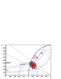
Figure 1: Fits of the parameters $\bar{\rho}$, $\bar{\eta}$ to the 2003 values of the constraints afecting the CKM matrix in the SM and in the MSSM case. The dotted lines indicate the regions of 1$\sigma$ for the different constriants, except in the case of $\sin 2\beta$ where we have ploted the 2$\sigma$ region as a reference. In $|\epsilon_{K}|$ the red(light) lines represent this constraint in the SM without new physics contributions. The grey(dark) lines represent the constraint in the MSSM case where we enlarge the error a 20% as explained in the text. The coloured (different grey tone) regions are the CL at 99%, 95% and 68% in the SM fit, while the wide continuous lines are the same CL in the MSSM case.

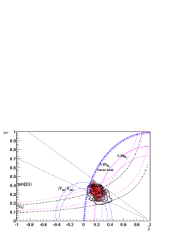
Figure 2: In this figure we assume that $20\%$ of the measured value of $\epsilon_{k}$ is due to SUSY contributions and we fit only the remaining $80\%$ of $\epsilon_{k}$. As we can see in this case we can reach lower values of $\bar{\eta}$, required for lower values of $\Phi_{2}$.

Appendix B Neutrino mass matrix, Model I

With the seesaw mechanism, we obtain the low energy effective neutrino mass matrix $\chi^{\nu}$ as,

$$\chi^{\nu}=Y^{\nu}M^{-1}_{R}(Y^{\nu})^{T}=Y^{\nu}L_{M}(M_{R})^{-1}_{\rm diag}L^{T}_{M}(Y^{\nu})^{T},$$ (169)

where $L_{M}$ is the complex orthogonal matrix diagonalising $M_{R}$ and up to ${\cal{O}}(\varepsilon^{5.5})$,

$$L_{M} \simeq \left(\begin{array}[]{ccc}ic_{12}e^{-i(\delta^{\prime}-4\alpha_{u})}&s_{12}e^{-i(\delta^{\prime}-4\alpha_{u})}&0\\ -is_{12}e^{-i4\alpha_{u}}&c_{12}e^{-i4\alpha_{u}}&\eta_{1}\varepsilon^{2.75}e^{-i4\alpha_{u}}\\ is_{12}\eta_{1}\varepsilon^{2.75}&-c_{12}\eta_{1}\varepsilon^{2.75}&1\end{array}\right)$$ (173)

where $s_{12}\simeq\frac{\lambda}{\rho}\varepsilon^{1/4}$ and $c_{12}\simeq 1-\frac{\lambda^{2}}{2\rho^{2}}\varepsilon^{1/2}$. Now $(M_{R})^{-1}_{\rm diag}=\mbox{Diag.}(\frac{\rho}{\lambda^{2}\varepsilon^{6}},\frac{1}{\rho\varepsilon^{5.5}},1)$ and

$$(Y^{\nu})^{\prime}~{}~{}=~{}~{}~{}~{}Y^{\nu}\cdot L_{M}~{}~{}\simeq~{}~{}\left(\begin{array}[]{ccc}e^{i(\delta^{u}-4\alpha_{u})}&&\\ &e^{-i\beta_{3}}&\\ &&1\end{array}\right)~{}\cdot~{}~{}~{}~{}~{}~{}~{}~{}~{}~{}~{}~{}~{}~{}~{}~{}~{}~{}~{}~{}~{}~{}~{}~{}~{}~{}~{}~{}~{}$$ (177)

$$\left(\begin{array}[]{ccc}-is_{12}\varepsilon^{3}(X_{1}-X_{2}\eta_{1}\varepsilon^{2.75}e^{i\varphi})&c_{12}\varepsilon^{3}(X_{1}-X_{2}\eta_{1}\varepsilon^{2.75}e^{i\varphi})&\varepsilon^{3}(X_{2}e^{i\varphi}+X_{1}\eta_{1}\varepsilon^{2.75})\\ i\varepsilon^{3}(c_{12}X_{1}+s_{12}\eta\eta_{1}\varepsilon^{2.5}e^{i\varphi})&\varepsilon^{3}(s_{12}X_{1}-c_{12}\eta\eta_{1}\varepsilon^{2.5}e^{i\varphi})&\eta\varepsilon^{2.75}e^{i\varphi}\\ ic_{12}\varepsilon^{3}X_{2}-is_{12}(\eta-\eta_{1})\varepsilon^{2.75}&s_{12}\varepsilon^{3}X_{2}+c_{12}(\eta-\eta_{1})\varepsilon^{2.75}&1\\ \end{array}\right),$$ (181)

where we have defined $\rho=(\eta_{2}-\eta_{1}^{2})$, $X_{1}=(1+X)$, $X_{2}=(1-X)$ and the phase $\varphi=4\alpha_{u}+\beta_{3}$. Notice that the structure of the rotated Yukawa matrix has allowed us to extract a diagonal matrix of phases such that only $\varphi$ appears in the remaining matrix. Now we can obtain the elements of the effective neutrino mass matrix $m^{\nu}_{LL}=v_{2}^{2}P\cdot\chi^{\nu}\cdot P$ with $P=\mbox{Diag}(e^{i(\delta^{u}-4\alpha_{u})},e^{-i\beta_{3}},1)$ and,

$$\chi^{\nu}\simeq$$ (182)

$$\left(\begin{array}[]{ccc}-\frac{\rho}{\lambda^{2}}s_{12}^{4}X_{1}&\frac{\rho}{\lambda^{2}}s_{12}c_{12}X_{1}^{2}(1+s_{12}^{2})&\frac{\rho}{\lambda^{2}}s_{12}X_{1}\left(c_{12}X_{2}(1+s_{12}^{2})-\frac{(\eta-\eta_{1})\lambda}{\rho}s_{12}^{2}\right)\\ &-\frac{\rho}{\lambda^{2}}X_{1}^{2}c_{12}^{2}&-\frac{\rho}{\lambda^{2}}\left(X_{1}X_{2}c_{12}^{2}-\frac{(\eta-\eta_{1})\lambda}{\rho}c_{12}(1+s_{12}^{2})X_{1}\right)\\ &&1+2\frac{(\eta-\eta_{1})}{\lambda}c_{12}(1+s_{12}^{2})X_{2}-\frac{\rho}{\lambda^{2}}c_{12}^{2}X_{2}^{2}-\frac{(\eta-\eta_{1})^{2}}{\rho}s_{12}^{2}\end{array}\right)$$ (186)

However this is the neutrino mass matrix before diagonalisation of charged lepton Yukawas. To obtain the lepton mixings and especially the $CP$ violating phases relevant for phenomenology, it is more convenient to go to the basis of real and diagonal charged lepton masses. To reach this basis we must rotate and rephase this effective neutrino mass matrix: $\chi^{\prime}=L^{l\dagger}\cdot P\cdot\chi\cdot P\cdot L^{l*}$, with,

$$L^{l}\equiv P^{\prime}\cdot U=\left(\begin{array}[]{ccc}e^{i\delta^{d}}&&\\ &1&\\ &&e^{i(2\chi-\beta_{3})}\end{array}\right)\cdot\left(\begin{array}[]{ccc}1&\bar{\varepsilon}\frac{X_{1}}{\Sigma_{e}}&0\\ -\bar{\varepsilon}\frac{X_{1}}{\Sigma_{e}}&1&0\\ 0&0&1\end{array}\right)+{\cal{O}}(\bar{\varepsilon}^{2})$$ (193)

which is enough for our purposes. So, we have,

$$\chi^{\prime}=\tilde{P}\cdot\left(\begin{array}[]{ccc}1&-\bar{\varepsilon}\frac{X_{1}}{\Sigma_{e}}e^{i\varphi_{L}}&0\\ \bar{\varepsilon}\frac{X_{1}}{\Sigma_{e}}e^{-i\varphi_{L}}&1&0\\ 0&0&1\end{array}\right)\cdot\chi\cdot\left(\begin{array}[]{ccc}1&\bar{\varepsilon}\frac{X_{1}}{\Sigma_{e}}e^{-i\varphi_{L}}&0\\ -\bar{\varepsilon}\frac{X_{1}}{\Sigma_{e}}e^{i\varphi_{L}}&1&0\\ 0&0&1\end{array}\right)\cdot\tilde{P}$$ (200)

where $\varphi_{L}=-2\alpha_{d}-2\alpha_{u}+\beta_{3}$ and $\tilde{P}=\mbox{Diag}(e^{i(-2\alpha_{d}-2\alpha_{u})},e^{-i\beta_{3}},e^{i(-2\chi+\beta_{3})})$

References

-
[1]
For a review and further references see:
G. G. Ross, “Models of Fermion masses”, Published in TASI 2000 ed. J. L. Rosner (World Scientific, New Jersey, 2001) - [2] A. Masiero and O. Vives, Ann. Rev. Nucl. Part. Sci. 51 (2001) 161 [arXiv:hep-ph/0104027].
- [3] S. F. King and G. G. Ross, Phys. Lett. B 520 (2001) 243 [arXiv:hep-ph/0108112].
- [4] G. G. Ross and L. Velasco-Sevilla, Nucl. Phys. B 653 (2003) 3 [arXiv:hep-ph/0208218].
- [5] S. F. King and G. G. Ross, arXiv:hep-ph/0307190.
- [6] R. G. Roberts, A. Romanino, G. G. Ross and L. Velasco-Sevilla, Nucl. Phys. B 615 (2001) 358 [arXiv:hep-ph/0104088].
- [7] M. Dine, R. G. Leigh and D. A. MacIntire, Phys. Rev. Lett. 69 (1992) 2030 [arXiv:hep-th/9205011].
-
[8]
Y. Nir and R. Rattazzi,
Phys. Lett. B 382 (1996) 363
[arXiv:hep-ph/9603233];
J. L. Chkareuli, C. D. Froggatt and H. B. Nielsen, Nucl. Phys. B 626 (2002) 307 [arXiv:hep-ph/0109156]. - [9] P. Ramond, R. G. Roberts and G. G. Ross, Nucl. Phys. B 406 (1993) 19 [arXiv:hep-ph/9303320].
- [10] R. Gatto, G. Sartori and M. Tonin, Phys. Lett. B 28 (1968) 128.
- [11] C. D. Froggatt and H. B. Nielsen, Nucl. Phys. B 147 (1979) 277.
-
[12]
M. Dine, R. G. Leigh and A. Kagan,
Phys. Rev. D 48 (1993) 4269
[arXiv:hep-ph/9304299];
A. Pomarol and D. Tommasini, Nucl. Phys. B 466 (1996) 3 [arXiv:hep-ph/9507462];
L. J. Hall and H. Murayama, Phys. Rev. Lett. 75 (1995) 3985 [arXiv:hep-ph/9508296];
R. Barbieri, G. R. Dvali and L. J. Hall, Phys. Lett. B 377 (1996) 76 [arXiv:hep-ph/9512388];
Z. Berezhiani, Phys. Lett. B 417 (1998) 287 [arXiv:hep-ph/9609342];
E. Dudas, C. Grojean, S. Pokorski and C. A. Savoy, Nucl. Phys. B 481 (1996) 85 [arXiv:hep-ph/9606383];
R. Barbieri, L. J. Hall, S. Raby and A. Romanino, Nucl. Phys. B 493 (1997) 3 [arXiv:hep-ph/9610449]. -
[13]
Y. Nir and N. Seiberg,
Phys. Lett. B 309 (1993) 337
[arXiv:hep-ph/9304307];
M. Leurer, Y. Nir and N. Seiberg, Nucl. Phys. B 420 (1994) 468 [arXiv:hep-ph/9310320];
Y. Nir and G. Raz, Phys. Rev. D 66 (2002) 035007 [arXiv:hep-ph/0206064]. -
[14]
E. Dudas, S. Pokorski and C. A. Savoy,
Phys. Lett. B 356 (1995) 45
[arXiv:hep-ph/9504292];
E. Dudas, S. Pokorski and C. A. Savoy, Phys. Lett. B 369 (1996) 255 [arXiv:hep-ph/9509410];
I. Jack, D. R. T. Jones and R. Wild, Phys. Lett. B 580 (2004) 72 [arXiv:hep-ph/0309165];
S. F. King and I. N. R. Peddie, arXiv:hep-ph/0312237. - [15] S. F. King, I. N. R. Peddie, G. G. Ross, L. Velasco-Sevilla and O. Vives, work in progress.
- [16] H. Leutwyler, Nucl. Phys. Proc. Suppl. 94 (2001) 108 [arXiv:hep-ph/0011049].
- [17] E. Gamiz, M. Jamin, A. Pich, J. Prades and F. Schwab, JHEP 0301 (2003) 060 [arXiv:hep-ph/0212230].
-
[18]
J. Penarrocha and K. Schilcher,
Phys. Lett. B 515 (2001) 291
[arXiv:hep-ph/0105222];
J. Erler and M. x. Luo, Phys. Lett. B 558 (2003) 125 [arXiv:hep-ph/0207114];
M. Eidemuller, Phys. Rev. D 67 (2003) 113002 [arXiv:hep-ph/0207237];
B. L. Ioffe and K. N. Zyablyuk, Eur. Phys. J. C 27 (2003) 229 [arXiv:hep-ph/0207183]. - [19] G. Rodrigo, A. Pich and A. Santamaria, Phys. Lett. B 424 (1998) 367 [arXiv:hep-ph/9707474].
- [20] F. Gabbiani, E. Gabrielli, A. Masiero and L. Silvestrini, Nucl. Phys. B 477 (1996) 321 [arXiv:hep-ph/9604387].
- [21] K. Hagiwara et al. [Particle Data Group Collaboration], Phys. Rev. D 66 (2002) 010001.
- [22] M. Olechowski and S. Pokorski, Phys. Lett. 257 (1991) 388.
- [23] V. D. Barger, M. S. Berger and P. Ohmann, Phys. Rev. D 47 (1993) 2038 [arXiv:hep-ph/9210260].
- [24] R. D. Peccei and H. R. Quinn, Phys. Rev. Lett. 38 (1977) 1440.
- [25] L. Velasco-Sevilla, JHEP 0310 (2003) 035 [arXiv:hep-ph/0307071].
- [26] S. F. King, Phys. Lett. B 439 (1998) 350 [arXiv:hep-ph/9806440]; S. F. King, Nucl. Phys. B 576 (2000) 85 [arXiv:hep-ph/9912492]; S. F. King, JHEP 0209 (2002) 011 [arXiv:hep-ph/0204360].
- [27] S. F. King, Phys. Rev. D 67 (2003) 113010 [arXiv:hep-ph/0211228].
-
[28]
S. Davidson and A. Ibarra,
Nucl. Phys. B 648 (2003) 345
[arXiv:hep-ph/0206304];
J. R. Ellis and M. Raidal, Nucl. Phys. B 643 (2002) 229 [arXiv:hep-ph/0206174];
S. Pascoli, S. T. Petcov and W. Rodejohann, Phys. Rev. D 68 (2003) 093007 [arXiv:hep-ph/0302054];
A. Ibarra and G. G. Ross, Phys. Lett. B 575 (2003) 279 [arXiv:hep-ph/0307051];
S. Davidson and R. Kitano, arXiv:hep-ph/0312007. - [29] T. Kobayashi and O. Vives, Phys. Lett. B 506 (2001) 323 [arXiv:hep-ph/0011200].
- [30] S. Abel, S. Khalil and O. Lebedev, Phys. Rev. Lett. 89 (2002) 121601 [arXiv:hep-ph/0112260].
- [31] G. G. Ross and O. Vives, Phys. Rev. D 67 (2003) 095013 [arXiv:hep-ph/0211279].
- [32] S. M. Barr and A. Masiero, Phys. Rev. D 38 (1988) 366.
- [33] A. Masiero, M. Piai and O. Vives, Phys. Rev. D 64 (2001) 055008 [arXiv:hep-ph/0012096].
- [34] O. Lebedev, Phys. Rev. D 67 (2003) 015013 [arXiv:hep-ph/0209023].
- [35] D. Becirevic et al., Nucl. Phys. B 634 (2002) 105 [arXiv:hep-ph/0112303].
-
[36]
K. Abe [Belle Collaboration],
arXiv:hep-ex/0308035,
B. Aubert et al. [BABAR Collaboration], arXiv:hep-ex/0207070. -
[37]
E. Lunghi and D. Wyler,
Phys. Lett. B 521 (2001) 320
[arXiv:hep-ph/0109149];
T. Goto, Y. Okada, Y. Shimizu, T. Shindou and M. Tanaka, Phys. Rev. D 66, 035009 (2002) [arXiv:hep-ph/0204081];
D. Chang, A. Masiero and H. Murayama, Phys. Rev. D 67, 075013 (2003) [arXiv:hep-ph/0205111];
S. Khalil and E. Kou, Phys. Rev. D 67 (2003) 055009 [arXiv:hep-ph/0212023];
S. Baek, Phys. Rev. D 67, 096004 (2003) [arXiv:hep-ph/0301269];
J. Hisano and Y. Shimizu, Phys. Lett. B 565, 183 (2003) [arXiv:hep-ph/0303071];
K. Agashe and C. D. Carone, Phys. Rev. D 68, 035017 (2003) [arXiv:hep-ph/0304229];
G. L. Kane, P. Ko, H. b. Wang, C. Kolda, J. h. Park and L. T. Wang, Phys. Rev. Lett. 90 (2003) 141803 [arXiv:hep-ph/0304239]. - [38] M. Ciuchini, E. Franco, A. Masiero and L. Silvestrini, Phys. Rev. D 67 (2003) 075016 [arXiv:hep-ph/0212397].
-
[39]
I. Masina and C. A. Savoy,
Nucl. Phys. B 661 (2003) 365
[arXiv:hep-ph/0211283];
J. I. Illana and M. Masip, Phys. Rev. D 67 (2003) 035004 [arXiv:hep-ph/0207328];
M. Ciuchini, A. Masiero, L. Silvestrini, S. K. Vempati and O. Vives, arXiv:hep-ph/0307191. - [40] S. Khalil, T. Kobayashi and O. Vives, Nucl. Phys. B 580 (2000) 275 [arXiv:hep-ph/0003086].
-
[41]
A. Masiero and O. Vives,
Phys. Rev. Lett. 86 (2001) 26
[arXiv:hep-ph/0007320];
A. E. Faraggi and O. Vives, Nucl. Phys. B 641 (2002) 93 [arXiv:hep-ph/0203061]. - [42] M. Battaglia et al., arXiv:hep-ph/0304132.
- [43] Heavy Flavor Averaging Group. Results Summer 2003. Available at http://www.slac.stanford.edu/xorg/hfag/
- [44] D. Becirevic, arXiv:hep-ph/0310072.