Moments of semileptonic $B$ decay distributions in the $1/m_{b}$ expansion

We report the OPE-based predictions for a number of lepton energy and hadronic mass moments in the inclusive semileptonic $B\!\to\!X_{c}\,\ell\nu$ decays with a lower cut on the charged lepton energy. We rely on the direct OPE approach where no expansion in the charm mass is employed and the theoretical input is a limited set of underlying OPE parameters including $m_{b}$ and $m_{c}$. A Wilsonian treatment with a ‘hard’ cutoff is applied using running low-scale masses $m_{Q}(\mu)$ and kinetic expectation value $\mu_{\pi}^{2}(\mu)$. This leaves for perturbative corrections only genuinely short-distance effects and makes them numerically small. Predictions are also given for the modified hadronic moments of the kinematic variable ${\cal N}_{X}^{2}$ which is a combination of $M_{X}^{2}$ and $E_{X}$. Measurement of such moments would allow a more reliable extraction of higher-order nonperturbative heavy quark parameters from experiment.

^∗On leave of absence from St. Petersburg Nuclear Physics Institute, Gatchina, St. Petersburg 188300, Russia

1 Introduction and motivation

The heavy quark expansion based on the local Operator Product Expansion (OPE) [2, 3, 4] allows to accurately calculate sufficiently inclusive decay probabilities, incorporating bound-state and hadronization effects in terms of a limited number of physical heavy quark parameters (for details, see the review [5]). Inclusive $B$ decay distributions – in particular those related to $b\!\to\!c\,\ell\nu$ transitions – represent a portal to a precise determination of these parameters [6, 7], and lepton energy moments and moments of hadronic mass and/or energy are among the most interesting quantities. The main ingredients for their computations have been around for some time (see [3, 8, 9, 10, 11, 12, 13, 14]). Several numerical applications can be found in the literature, for moments with or without cuts on the charged lepton energy (see [15, 16, 17] and references therein) often dictated by the reality of experimental measurements. The present study differs from and complements previous reports in a number of aspects.

First, we make use of the robust approach advocated in [18, 19]; in particular, we do not invoke an expansion in $1/m_{c}$ which has plagued the reliability of many earlier applications of the heavy quark expansion. Moreover, in our approach only the heavy quark parameters relevant to inclusive decay rates are invoked. This reduces the number of new objects appearing at order $1/m_{Q}^{3}$ from six to two and eliminates poorly known non-local correlators. An extended set of experimental moments allows to constrain all relevant parameters provided model-independent bounds [20] are incorporated.

We also rely on heavy quark parameters which are renormalized a la Wilson and depend explicitly on a ‘hard’ normalization scale $\mu$ which we set equal to $1\,\mbox{GeV}$. Primarily, this refers to the heavy quark masses $m_{b}(\mu)$ and $m_{c}(\mu)$ and to the kinetic expectation value $\mu_{\pi}^{2}(\mu)$. On the theoretical side, this is necessary both to meaningfully assign them definite values and to apply exact heavy quark inequalities. On the practical side this renders perturbative corrections well-behaved and moderate in size. Absence of large higher order corrections is crucial for a meaningful extraction of the nonperturbative parameters.

The direct use of the underlying set of heavy quark parameters reveals what a particular moment is actually measuring or constraining, and simplifies considerably the task of estimating the theoretical accuracy, often the subject of controversial claims [21]. It is worth reminding [7] in this respect that the inclusive decays cannot depend on non-local correlators often appearing in other applications of the heavy quark expansion, and there is no way to constrain them directly studying only inclusive $B$ decays.

The important motivation behind the present study is to make available a code for evaluating the various distributions, which is not bound to specific technical assumptions, for instance the use of meson mass relations, and is flexible enough to allow a meaningful investigation of the theoretical uncertainty using different options (see Section 3). The detailed analytic expressions will be given in Ref. [22], while here we limit ourselves with presenting easy numerical recipes and a discussion of the main points.

Finally, we present here predictions for the modified higher hadronic moments with a charged lepton energy cut, which can be measured in the experimental setup of the $B$ factories. They will allow to pinpoint higher-order nonperturbative expectation values with better accuracy and reliability.

2 Theoretical setup

All inclusive semileptonic $B$ decay distributions are described by a few $B$ decay structure functions $w_{i}(q_{0};q^{2})$, where $q^{\mu}$ is the four-momentum of the lepton pair; for massless leptons one has [9]

$$\frac{{\rm d}^{3}\Gamma}{{\rm d}E_{\ell\,}{\rm d}q^{2\,}{\rm d}q_{0}} \mbox{~{}}=\mbox{~{}} \frac{G_{F}^{2}|V_{cb}|^{2}}{32\pi^{4}}\,\vartheta\!\left(q_{0}\!-\!E_{\ell}\!-\!\mbox{$\frac{q^{2}}{4E_{\ell}}$}\right)\vartheta(E_{\ell})\,\vartheta(q^{2})\;\times$$ (1)

$$\mbox{\hskip 56.9055pt~{}}\left\{2q^{2}w_{1}+[4E_{\ell}(q_{0}\!-\!E_{\ell})\!-\!q^{2}]w_{2}+2q^{2}(2E_{\ell}\!-\!q_{0})w_{3}\right\}.$$

The OPE-based heavy quark expansion yields them in terms of (short-distance) quark masses and of the $B$-meson expectation values of local heavy quark operators. Accounting for the latter through $D\!=\!6$, the set of input parameters for our evaluation of the moments includes therefore $m_{b}$, $m_{c}$, $\mu_{\pi}^{2}$, $\mu_{G}^{2}$, $\tilde{\rho}_{D}^{3}$ and $\rho_{LS}^{3}$. Hadronic mass moments kinematically depend also on the $B$ meson mass $M_{B}$ for which the experimental value $5.279\,\mbox{GeV}$ is employed. In practice, it appears in the combination $\bar{\Lambda}^{\prime}\!\equiv\!M_{B}\!-\!m_{b}$. As mentioned above, the input heavy quark parameters depend on the normalization point $\mu$ for which we adopt $1\,\mbox{GeV}$.

The general structure of the OPE expressions for moments is described elsewhere [16, 22]. Here we give some technical details of our calculations.

Charged lepton energy moments are computed as the ratios

$$M_{\ell}^{(n)}(E_{\rm cut})=\frac{\int_{E_{\rm cut}}E_{\ell}^{n}\frac{{\rm d}\Gamma}{{\rm d}E_{\ell}}\,{\rm d}E_{\ell}}{\int_{E_{\rm cut}}\frac{{\rm d}\Gamma}{{\rm d}E_{\ell}}\,{\rm d}E_{\ell}}\;.$$ (2)

Both numerator and denominator have been computed through order $1/m_{b}^{3}$ compared to the leading partonic result; perturbative corrections are included from terms $\alpha_{s}$ and $\beta_{0}\alpha_{s}^{2}$, and the ratio has been expanded in both perturbative and nonperturbative corrections. Since perturbative corrections in the Wilsonian scheme are suppressed, an alternative procedure with separate numerical evaluation of both numerator and denominator would yield a close result. Perturbative effects are expressed in terms of $\alpha_{s}^{\overline{\rm MS}}(m_{b})$ for which we adopt $0.22$ as central value.

Hadronic invariant mass squared $M_{X}^{2}$ in the OPE appears as a special choice in a one-parameter family of kinematic variables

$${\cal M}^{2}(L_{\nu})\mbox{~{}} = \mbox{~{}}(L_{\nu}\!+\!m_{b}v_{\nu}\!-\!q_{\nu})^{2}=L^{2}+(m_{b}v_{\nu}\!-\!q_{\nu})^{2}+2L_{\nu}(m_{b}v_{\nu}\!-\!q_{\nu})\,,$$ (3)

$$\mbox{\hskip 14.22636pt~{}}(m_{b}v_{\nu}\!-\!q_{\nu})^{2}\equiv m_{x}^{2},\;\;\;(m_{b}\!-\!q_{0})\equiv e_{x}\mbox{\hskip 28.45274pt~{}}$$

corresponding to $L_{\nu}\!=\!\bar{\Lambda}^{\prime}v_{\nu}$, where $v_{\nu}\!=\!\frac{P^{B}_{\nu}}{M_{B}}\!=\!(1,{\bf 0})\,$ is the $B$ four-velocity, and $m_{x}^{2}$ and $e_{x}$ have the meaning of invariant mass squared and energy in the hadron sector at the quark decay level, $e_{x}\!=\!E_{X}\!-\!\bar{\Lambda}^{\prime}$. The OPE computes $m_{x}^{2}$ and $e_{x}$ much in the same way as lepton energy moments; therefore averages of $M_{X}^{2}$ and its powers are generally polynomials in $(M_{B}\!-\!m_{b})$, with the coefficients computed in the local OPE [23]. The latter are various mixed moments $\langle e_{x}^{k}\,m_{x}^{2n}\rangle$ derived from Eq. (1).

The variable ${\cal M}^{2}$ represents an observable for arbitrary $L_{\nu}$. Being a combination of hadronic invariant mass and hadronic energy (and most generally of spacelike momentum), it can also be viewed as conventional “hadronic” invariant mass square if one considers not the decay of an isolated $B$ meson, but rather of a compound of $B$ combined with a non-interacting ‘spurion’ particle having momentum $L_{\nu}\!-\!(P^{B}_{\nu}\!-\!m_{b}v_{\nu})$. From the OPE perspective, however, the inclusive probabilities appear as in the decay of the $b$ quark, while the momentum associated with the light cloud looks like a spurion. The native object for the OPE is therefore ${\cal M}^{2}(L_{\nu})$ with vanishing $L_{\nu}$, rather than $L_{\nu}\!=\!\bar{\Lambda}^{\prime}v_{\nu}$ which yields $M_{X}^{2}$.

It turns out that for higher hadronic moments the generalized moments with $L_{\nu}\!\ll\!\bar{\Lambda}^{\prime}$ are advantageous, they are better controlled theoretically and more directly sensitive to higher-dimension expectation values. To utilize this advantage we consider, along with $M_{X}^{2}$ the modified moments, i.e. those of

$${\cal N}_{X}^{2}=M_{X}^{2}-2\tilde{\Lambda}E_{X}+\tilde{\Lambda}^{2}$$ (4)

with $\tilde{\Lambda}\!=\!0.65\,\mbox{GeV}$, close to the anticipated value of $\bar{\Lambda}^{\prime}$. In this case ${\cal N}_{X}^{2}\!-\!m_{c}^{2}$ approximates the quark virtuality, for which higher moments with respect to average are intrinsically related to higher-dimension expectation values. (The last constant term in Eq. (4) does not affect such moments.) In our approach computing these modified moments does not require a new analysis – they are given by simply replacing $M_{B}$ by $M_{B}\!-\!\tilde{\Lambda}$.

The higher moments of the decay distributions – in particular those of the hadronic invariant mass – are more informative when considered with respect to the average, say $\langle(M_{X}^{2}\!-\!\langle M_{X}^{2}\rangle)^{2}\rangle$, $\langle(M_{X}^{2}\!-\!\langle M_{X}^{2}\rangle)^{3}\rangle$, or similar moments for ${\cal N}_{X}^{2}$. These moments are the focus of our study. Since this may complicate to some extent the experimental error analysis, we also present similar numerical results for the moments evaluated with respect to a fixed hadronic mass, for which we take $4\,\mbox{GeV}^{2}$ in the case of $M_{X}^{2}$-moments and $1.35\,\mbox{GeV}^{2}$ for ${\cal N}_{X}^{2}$ ones.

Power corrections in moments with lepton cut are obtain directly integrating the published heavy quark structure functions. The emerging analytic expressions are not too complicated, but lengthy and consist of many terms, especially for higher hadronic moments. We will present them in a dedicated publication [22]. Perturbative corrections are cumbersome and require numerical integrations. At the same time, in our approach utilizing a ‘hard’ separation between short- and long-distance effects they are numerically quite small. (For instance, it follows from the tables in the Appendix that including perturbative corrections in $\langle M_{X}^{2}\rangle$ has the same impact as decreasing $m_{b}$ by $15\,\mbox{MeV}$, or as decreasing $\mu_{\pi}^{2}$ by $0.02\,\mbox{GeV}^{2}$ in $\langle(M_{X}^{2}\!-\!\langle M_{X}^{2}\rangle)^{2}\rangle$.) Therefore we evaluate hadronic moments to the first order in $\alpha_{s}$ using the value $\alpha_{s}\!=\!0.3$ (average gluon virtuality in $B$ decays is lower than $m_{b}$). Moreover, in the present paper we evaluated perturbative shifts in the hadronic moments neglecting the cut on the lepton energy. This seems to be a legitimate approximation since at $E_{\rm cut}\!=\!0$ they are small and do not exceed the expected accuracy, which is limited by other neglected effects. This element will be improved in Ref. [22].

Unlike the case of lepton moments, for power-suppressed terms we do not use the expanded form of the ratios that form the moments, nor drop any power-like terms generated by $\mu_{\pi}^{2}$, $\mu_{G}^{2}$, $\rho_{D}^{3}$ and $\rho_{LS}^{3}$ wherever they appear. In particular, this implies that we would not include $M_{B}\!-\!m_{b}$ (or its analogue $M_{B}\!-\!m_{b}\!-\!\tilde{\Lambda}$ for ${\cal N}_{X}^{2}$-moments) into counting powers of $\Lambda_{\rm QCD}$. This is natural since that entry is external to the OPE for inclusive probabilities and it can take arbitrary values, both much larger and much smaller than $\Lambda_{\rm QCD}$, as illustrated by the modified hadronic moments. Similarly, in the perturbative corrections terms like $\sim\!\alpha_{s}\mu_{\pi}^{2}$, $\;\alpha_{s}\mu_{G}^{2}$ etc. are not retained, but those $\sim\!\alpha_{s}\bar{\Lambda}^{k}$ without nonperturbative expectation values are legitimately kept for arbitrary power $k$.

In this note we present our numerical results in a simplified form, using the following reference values of the parameters

$$m_{b}\!=\!4.6\,\mbox{GeV},\;\;\;m_{c}\!=\!1.2\,\mbox{GeV},\;\;\;\mu_{\pi}^{2}\!=\!0.4\,\mbox{GeV}^{2},\;\;\;\mu_{G}^{2}\!=\!0.35\,\mbox{GeV}^{2},\;$$

$$\tilde{\rho}_{D}^{3}\!=\!0.1\,\mbox{GeV}^{3},\;\;\;\;\rho_{LS}^{3}\!=\!-0.15\,\mbox{GeV}^{3},$$ (5)

and providing the coefficients for the linear extrapolation in these values from this base point. Such linearized extrapolations appear sufficiently accurate for reasonable values of the parameters. The tables summarizing our results are given in the Appendix. Yet this is no more than the simplest compact way of communicating our results (for instance, we drew plots using the complete expressions rather than interpolations). The numerical evaluations for other central values, more accurate interpolating tables, or compact Mathematica or FORTRAN programs evaluating them are available upon request, and will be provided with Ref. [22].

Measured in experiment are also non-integer moments of $M_{X}^{2}$, most notably $\langle M_{X}\rangle$ and $\langle M_{X}^{3}\rangle$ [24]. They do not arise naturally in the $1/m_{b}$ expansion, as illustrated by the limit $m_{c}\!\to\!0$ which is analogous to the decay $B\!\to\!X_{s}+\gamma$; fractional photon energy moments are not given there by the expectation values of local heavy quark operators. For $B\!\to\!X_{c}\,\ell\nu$, the OPE would involve an expansion in $1/m_{c}$, as can also be seen from

$$\langle M_{X}^{\nu}\rangle=\left(\langle M_{X}^{2}\rangle\right)^{\frac{\nu}{2}}\left[1+\sum_{k=2}^{\infty}\raisebox{-2.0pt}{\mbox{{\large$C$}}}_{\!{}_{\frac{\nu}{2}}}^{{}^{\,k}}\,\frac{\langle(M_{X}^{2}-\langle M_{X}^{2}\rangle)^{k}\rangle}{\langle M_{X}^{2}\rangle^{k}}\right];$$ (6)

for integer moments with $\nu\!=\!2n$ the sum contains only terms through $k\!=\!n$ and stops before $\langle M_{X}^{2}\rangle$ enters the denominator.

Having computed three first (integer) hadronic moments, we truncated the sum in Eq. (6) after $k\!=\!3$. Although incomplete, at the actual value of the charm mass this truncated expansion appears a sufficiently good numerical approximation for $\nu\!=\!1$ and $\nu\!=\!3$; the omitted terms seem significantly below the actual theoretical accuracy in evaluating the integer moments involved.

In fact, $M_{X}^{2}$ contains the dominant term $2\bar{\Lambda}^{\prime}e_{x}$ as well as the perturbative bremsstrahlung contribution, and both effects can be computed explicitly for arbitrary $\nu$ without truncating the series in Eq. (6). The numerical impact of this resummation turns out totally negligible numerically. Moreover, while the term $2\bar{\Lambda}^{\prime}e_{x}$ dominates $\langle M_{X}^{2}\rangle$, it is subdominant in the higher moments with respect to $\langle M_{X}^{2}\rangle$.

Figure 1: Average hadronic invariant mass squared $\langle M_{X}^{2}\rangle$ at different lepton energy cuts, for the heavy quark parameters of Eq. (5). Figure 2: Second invariant mass moment $\langle[M_{X}^{2}\!-\!\langle M_{X}^{2}\rangle]^{2}\rangle$ (red) and second modified hadronic moment $\langle[{\cal N}_{X}^{2}\!-\!\langle{\cal N}_{X}^{2}\rangle]^{2}\rangle$ (blue), in the same setting.

For illustration we give a few plots showing dependence of the hadronic mass moments on the lepton energy cut, at the central values of heavy quark parameters. Fig. 1 depicts $\langle M_{X}^{2}\rangle$, Fig. 2 addresses $\langle(M_{X}^{2}-\langle M_{X}^{2}\rangle)^{2}\rangle$ and $\langle({\cal N}_{X}^{2}-\langle{\cal N}_{X}^{2}\rangle)^{2}\rangle$. Non-integer $M_{X}^{2}$ moments are shown in Fig. 3 where we actually plot the corresponding powers of the moments having dimension of mass, for $\nu=1,\,2,\,3,\,4,\,5$ and $6$. It shows that the full moments are by far dominated by the average invariant mass, with relatively small differences.

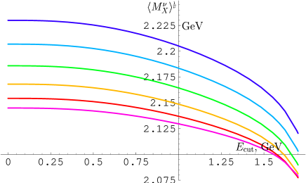
Figure 3: Different hadronic mass moments $\langle M_{X}^{\nu}\rangle^{\frac{1}{\nu}}$ for $\nu\!=\!1$ to $6$ (from lowest to highest), vs. lepton energy cuts; heavy quark parameters as in Eq. (5).

As the semileptonic decay rate is well measured only above certain energy $E_{\ell}$, the OPE predictions for the decay fraction

$$R^{*}(E_{\rm cut})=\frac{\int_{E_{\rm cut}}\frac{{\rm d}\Gamma}{{\rm d}E_{\ell}}\,{\rm d}E_{\ell}}{\int_{0}\frac{{\rm d}\Gamma}{{\rm d}E_{\ell}}\,{\rm d}E_{\ell}}$$ (7)

are helpful to reconstruct the overall $b\!\to\!c\,\ell\nu$ rate. Since the fraction of events cut out is small and they belong to the domain of low $E_{\ell}$ which is theoretically most robust, the predictions for $R^{*}$ are expected to be quite reliable.

3 Discussion

In the present paper we provide numerical expressions for the local OPE predictions of the charged lepton energy and hadronic mass moments with a lower cut on lepton energy. Two major aspects of our analysis have already been emphasized. First, no $1/m_{c}$ expansion is involved at any stage, and the $c$ quark mass can more or less be arbitrary, large or small within the same formalism. The second aspect is that we rely on well-defined running quark masses and $\mu_{\pi}^{2}$ normalized at the scale $1\,\mbox{GeV}$. (The scheme is often referred to as ‘kinetic’, however this name is elucidating only when applied to quark masses.) The advantages of this approach are well known, and can be readily seen from the applications presented here.

A quick comparison [25] with recent data [26, 27, 28] from DELPHI, BaBar and CLEO suggests agreement between this implementation of the OPE and experiment, with preferred values of the heavy quark parameters in the range expected theoretically. (Our estimates show that the expectations for two moments of the photon energy spectrum appear to fit the values reported by CLEO [29] once the ‘exponential’ effects discussed in Ref. [25] are adjusted for.) The dependence of the first and second hadronic mass squared moments on the lepton energy cut seems to be in a qualitative agreement with the preliminary data reported by BaBar and CLEO [27, 28]. The dedicated data analysis including possible fits to the predictions should, in our opinion be left for experiment, and we did not attempt this.

Once the heavy quark parameters are extracted from data, one can readily determine, for example, $|V_{cb}|$ from the measured semileptonic $b\!\to\!c$ decay width [19]:

$$\frac{|V_{cb}|}{0.0417}\mbox{~{}} = \mbox{~{}}\mbox{{\large$\left(\frac{{\rm Br}_{\rm sl}(B)}{0.105}\right)^{\!\frac{1}{2}}\left(\frac{1.55{\rm ps}}{\tau_{B}}\right)^{\frac{1}{2}}$}}\left(1\!-\!\mbox{{\small$4.8\,[{\rm Br}(B\!\to\!X_{u}\,\ell\nu)-0.0018]$}}\right)\cdot[1+0.30\,(\alpha_{s}(m_{b})\!-\!0.22)]\,$$ (8)

$$\mbox{\hskip 62.59605pt~{}}\times\,\left[1-0.66\left(m_{b}(1\,\mbox{GeV})\!-\!4.6\,\mbox{GeV}\right)+0.39\left(m_{c}(1\,\mbox{GeV})\!-\!1.15\,\mbox{GeV}\right)\qquad\right.$$

$$\mbox{\hskip 73.97716pt~{}}+0.013\left(\mu_{\pi}^{2}\!-\!0.4\,\mbox{GeV}^{2}\right)+0.09\left(\rho_{D}^{3}(1\,\mbox{GeV})\!-\!0.2\,\mbox{GeV}^{3}\right)$$

$$\mbox{\hskip 73.97716pt~{}}\left.+\,0.05\left(\mu_{G}^{2}\!-\!0.35\,\mbox{GeV}^{2}\right)-0.01\left(\rho_{LS}^{3}\!+\!0.15\,\mbox{GeV}^{3}\right)\right]\;.$$

It should be recalled, however, that $\rho_{D}^{3}(1\,\mbox{GeV})$ appearing in the above equation is related to $\tilde{\rho}_{D}^{3}$ employed in the present study by $\tilde{\rho}_{D}^{3}\simeq\rho_{D}^{3}(1\,\mbox{GeV})\!-\!0.1\,\mbox{GeV}^{3}$.

We do not intend to address here the question of theory accuracy for the moments to an extent commensurate to the analysis [19] of total $\Gamma_{\rm sl}(b\!\to\!c)$. Nevertheless, the numerical results presented in the Appendix allow a straightforward, if simplified, estimate of possible theory inaccuracies.

Since no perturbative corrections to the Wilson coefficients of nonperturbative operators have been computed so far, one can assume a related $\sim\!20\%$ uncertainty in the contributions due to $\mu_{\pi}^{2}$ and $\mu_{G}^{2}$ and a $\sim\!30\%$ uncertainty in those due to $\rho_{D}^{3}$ and $\rho_{LS}^{3}$. As perturbative corrections in hadronic moments are presently implemented only at first order in $\alpha_{s}$, the associated uncertainty can be assessed by varying $\alpha_{s}$ in a reasonable range; since the actual short-distance corrections selected by our Wilsonian treatment are moderate, we may conservatively vary the effective $\alpha_{s}$ between $0.2$ and $0.45$. To safeguard against possible accidental cancellations in perturbative corrections, one may assume an additional minimal uncertainty in $m_{b,c}$ of about $20\,\mbox{MeV}$. A similar ‘minimal uncertainty’ in $\mu_{\pi}^{2}$ is probably around $0.02\,\mbox{GeV}^{2}$.

The results we provide in the Appendix can be improved in several ways. The relevance of the improvements is essentially determined by the state of experiment. A more complete calculation of perturbative corrections in hadronic moments fully incorporating cuts in the lepton energy is the first on the list. All-order BLM resummation can be implemented in both lepton and hadron moments. There are ways to partially incorporate non-BLM second-order corrections without performing extensive new calculations. All these improvements in the perturbative corrections are not expected to essentially modify the final result in the Wilsonian scheme (see, e.g. the dedicated analysis of $\Gamma_{\rm sl}$ in Ref. [19]). Yet having them incorporated would add confidence in the present estimates and may allow to reduce the theoretical uncertainty.

A probe of the significance of second- and higher-order non-BLM corrections is already available by varying the normalization scale $\mu$ used for quark masses and $\mu_{\pi}^{2}$, $\rho_{D}^{3}$, while simultaneously running their values according to [30]

$$\frac{{\rm d}m_{Q}(\mu)}{{\rm d}\mu} \mbox{~{}}=\mbox{~{}} -\frac{16}{9}\frac{\alpha_{s}(M)}{\pi}\,\left(1+\frac{\alpha_{s}}{\pi}\left[\frac{\beta_{0}}{2}\left(\ln{\frac{M}{2\mu}}+\frac{5}{3}\right)-3\left(\frac{\pi^{2}}{6}-\frac{13}{12}\right)\right]\right)$$

$$\mbox{$-\frac{4}{3}\frac{\alpha_{s}(M)}{\pi}\frac{\mu}{m_{Q}}\left(1+\frac{\alpha_{s}}{\pi}\left[\frac{\beta_{0}}{2}\left(\ln{\frac{M}{2\mu}}+\frac{5}{3}\right)-3\left(\frac{\pi^{2}}{6}-\frac{13}{12}\right)\right]\right)$}\;,$$

$$\frac{{\rm d}\mu_{\pi}^{2}(\mu)}{{\rm d}\mu} \mbox{~{}}=\mbox{~{}} \mbox{\hskip 5.69054pt~{}}\mbox{$\frac{8}{3}\frac{\alpha_{s}(M)}{\pi}\mu\,\left(1+\frac{\alpha_{s}}{\pi}\left[\frac{\beta_{0}}{2}\left(\ln{\frac{M}{2\mu}}+\frac{5}{3}\right)-3\left(\frac{\pi^{2}}{6}-\frac{13}{12}\right)\right]\right)$}\;,$$

$$\frac{{\rm d}\rho_{D}^{3}(\mu)}{{\rm d}\mu} \mbox{~{}}=\mbox{~{}} \mbox{\hskip 5.69054pt~{}}4\mbox{$\frac{\alpha_{s}(M)}{\pi}\mu^{2}\left(1+\frac{\alpha_{s}}{\pi}\left[\frac{\beta_{0}}{2}\left(\ln{\frac{M}{2\mu}}+\frac{5}{3}\right)-3\left(\frac{\pi^{2}}{6}-\frac{13}{12}\right)\right]\right)$}\;,$$ (9)

where $M$ denotes the scale used for normalizing $\alpha_{s}$. In fact, in the future we will also explicitly adopt the Wilsonian $\rho_{D}^{3}(\mu)$ instead of $\tilde{\rho}_{D}^{3}$ currently used. Even the uncertainty obtained in this way may, however, not fully represent the uncalculated non-BLM corrections. A further option is using the $\overline{\rm MS}$ scheme for the charm mass, $\bar{m_{c}}(m_{c})$. With this choice, one could vary $\mu$ in a wider range to probe more quantitatively the actual hardness of a particular moment at a given $E_{\ell}$ cut, and a more direct comparison with $m_{c}$ extracted from different physical processes [31] would be possible. Since no constraints is imposed on $m_{b}\!-\!m_{c}$ through conventional mass relations like

$$m_{b}\!-\!m_{c}=\frac{M_{B}+3M_{B^{*}}}{4}-\frac{M_{D}+3M_{D^{*}}}{4}+\mu_{\pi}^{2}\left(\frac{1}{2m_{c}}\!-\!\frac{1}{2m_{b}}\right)+{\cal O}\left(\frac{1}{m_{Q}^{2}}\right)+...$$ (10)

the normalization point – or even the scheme itself – can be different for $m_{c}$ and $m_{b}$.

It should be emphasized that we have quoted in the Appendix what literally emerges from our OPE expressions, regardless of whether the cut on $E_{\ell}$ is mild or severe. However, if the cut is high, the effective hardness of the inclusive process degrades and the accuracy deteriorates. As has been argued [21, 25], the truncated expressions of practical OPE may not fully reflect this, while the so-called ‘exponential’ effects may become significant when $E_{\rm cut}$ exceeds $1.3$ to $1.5\,\mbox{GeV}$. The same reservation applies to the above simplified way to estimate theoretical accuracy – it largely leaves out this aspect. The additional cut-related theory errors are possibly insignificant below $1.35\,\mbox{GeV}$; they may not dominate even at $E_{\rm cut}=1.5\,\mbox{GeV}$ – yet this cannot be confidently derived from theory a priori.  The safest way to tackle them is to use as low $E_{\rm cut}$ as possible, not larger than $1.2\,\mbox{GeV}$.

A potential source of additional nonperturbative corrections are the so-called ‘intrinsic charm’, or IC contributions in the OPE, associated with non-vanishing expectation values of four-quark operators with charm fields $\bar{b}\Gamma c\,\bar{c}\Gamma b$. No allowance is presently reserved for them. It has been noted in Ref. [19] that their effect can mimic to some extent the contribution of the Darwin operator. We think therefore that at the moment theoretical constraints on $\rho_{D}^{3}$ should be used cautiously in the context of fits based on the OPE without possible IC contributions.

There are some conclusions we draw from our analysis. The moments under consideration seem to reliably (over)constrain a certain combination of the two heavy quark masses, approximately $m_{b}\!-\!0.6m_{c}$; the sensitivity to the individual masses is not high and they are subject to larger theoretical uncertainties.

The moments are only weakly sensitive to the spin-orbit expectation value $\rho_{LS}^{3}$, so it cannot be extracted from the data. On the other hand, $\rho_{LS}^{3}$ is reasonably constrained by a number of exact heavy quark sum rules which place model-independent bounds. Once they are taken into account, the associated uncertainty in the moments appears by far subdominant. Therefore, $\rho_{LS}^{3}$ does not have to be included in the fit and we suggest to use a fixed value $\rho_{LS}^{3}\!=\!-0.15\,\mbox{GeV}^{3}$, and to vary it within $\pm 0.1\,\mbox{GeV}^{3}$ to conservatively estimate the related uncertainty. This assumption would be further reinforced if the fits of data prefer values of the primary heavy quark parameters in the expected ranges

$$m_{b}(1\,\mbox{GeV})=4.60\pm 0.06\,\mbox{GeV},\qquad\mu_{\pi}^{2}(1\,\mbox{GeV})=0.45\pm 0.1\,\mbox{GeV}^{2},$$

$$0<\tilde{\rho}_{D}^{3}<0.15\,\mbox{GeV}^{3}\;\;\;\mbox{ or }\;\;\;0.1\,\mbox{GeV}^{3}<\rho_{D}^{3}(1\,\mbox{GeV})<0.25\,\mbox{GeV}^{3}\;,$$ (11)

see Refs. [5, 18, 32]; an updated review of different determinations of beauty and charm quark masses can be found in Ref. [31]. Similarly, since $\mu_{G}^{2}$ is accurately known, it should be set to $0.35\,\mbox{GeV}^{2}$ [33] and varied within $\pm 20\%$ to allow for the perturbative uncertainty in its Wilson coefficient.

Obtaining informative model-independent constraints on higher-dimension heavy quark parameters requires measurement of higher hadronic moments, at least the second and desirably the third one. Since these higher moments – when considered with respect to the average – depend strongly on higher-dimension expectation values, even a rough measurement of the variance and of the asymmetry parameter would yield precious information. One should be warned, however, that the theoretical accuracy one can realistically achieve for the higher moments of $M_{X}^{2}$ is limited, especially in the case of the third moment. On the other hand, the modified higher hadronic moments $\langle({\cal N}_{X}^{2}\!-\!\langle{\cal N}_{X}^{2}\rangle)^{2}\rangle$, $\langle({\cal N}_{X}^{2}\!-\!\langle{\cal N}_{X}^{2}\rangle)^{3}\rangle$ are better in this respect and more suitable to this purpose. We encourage experiments to pay closer attention to such combinations of $M_{X}^{2}$ and $E_{X}$ moments.

The actual assessment of the theoretical error in the calculation of the moments is a very subtle issue. We cannot do without mentioning a few important aspects.

First, there are strong correlations among theoretical uncertainties. After all, everything inclusive we compute is expressed in terms of only three structure functions which have physical properties like positivity, regardless of any dynamics. Because of these correlations, one should distinguish between the overall consistency of the fits to the various moments in the context of our formalism, and the concrete prediction for a certain moment. There are common uncertainties, like a systematic bias in $m_{b}$ or $\mu_{G}^{2}$, that would simply shift the fitted value of $m_{b}$ or $\mu_{G}^{2}$, but would not degrade the quality of the global fit, nor would they alter significantly the $E_{\rm cut}$-dependence [21]. At the same time, these uncertainties could still noticeably affect the numerical value of a particular moment.

On the other hand, there are uncertainties that affect each moment in a different way, for instance, unknown perturbative corrections to the Wilson coefficients of the nonperturbative operators, which are in principle different for every moment, and also depend on $E_{\rm cut}$. Therefore, simply varying the values of the heavy quark parameters uniformly in all observables may not represent realistically the uncertainty of the theoretical expressions, and an intermediate procedure may be required.

Having mentioned these complications of the theory error analysis, we would like to make a few suggestions that can be inferred from our study. For sufficiently low cut on $E_{\ell}$ a reasonable starting point is to estimate the theoretical accuracy in the moments just varying the values of the heavy quark parameters they depend upon in the ranges we have mentioned above Eq. (9). For higher moments, however, this should be applied to the moments with respect to average; the ordinary moments (around zero) would in this way exhibit strong theory error correlations. Clearly, allowance should be made for additional uncertainty once the cut is raised beyond $1.35\,\mbox{GeV}$.

In summary, we have seen that consistency checks between theory and emerging data should rely on robust theoretical elements, with additional assumptions reduced to minimum. Once agreement with theory is confirmed, and the domain and degree of applicability is verified experimentally (e.g., the safe interval for lepton cut), one can and should implement into the fit of data all the model-independent relations and bounds following from heavy quark sum rules. These are exact relations derived in QCD, and they are indispensable for a precision determination of the heavy quark parameters and for a stringent test of our theoretical tools.

Acknowledgments: We are indebted to many experimental colleagues from BaBar, in particular to Oliver Buchmueller and Urs Langenegger for important discussions which to a large extent initiated the present and further ongoing studies, and for important physics comments. The early stages of this investigation ascend to the analysis of LEP data, and we are grateful to DELPHI members, especially to M. Battaglia, M. Calvi and P. Roudeau for collaboration. N.U. is thankful to I. Bigi for many important discussions and suggestions. P.G. thanks the Theory Division of CERN where this work has been started. This work was supported in part by the NSF under grant number PHY-0087419 and by a Marie Curie Fellowship, contract No. HPMF-CT-2000-01048.

Appendix

The following tables give our numerical estimates for various moments. The general form for a generic moment ${\cal M}$ in question will be

$${\cal M}(m_{b},m_{c},\mu_{\pi}^{2},\mu_{G}^{2},\tilde{\rho}_{D}^{3},\rho_{LS}^{3};\alpha_{s})\mbox{~{}} = \mbox{~{}}V+B\,(m_{b}\!-\!4.6\,\mbox{GeV})+C\,(m_{c}\!-\!1.2\,\mbox{GeV})$$

$$\mbox{~{}}+P\,(\mu_{\pi}^{2}\!-\!0.4\,\mbox{GeV}^{2})+D\,(\tilde{\rho}_{D}^{3}\!-\!0.1\,\mbox{GeV}^{3})\qquad$$

$$\mbox{~{}}+G\,(\mu_{G}^{2}\!-\!0.35\,\mbox{GeV}^{2})+L\,(\rho_{LS}^{3}\!+\!0.15\,\mbox{GeV}^{3})+S\,(\alpha_{s}\!-\!0.22)\;;$$

$V$ represent the reference values obtained for the heavy quark parameters in Eq. (5). They have dimension of the moment ${\cal M}$ itself and the quoted number is in  GeV to the corresponding power. The values of all the coefficients $B$ to $S$ are likewise in the proper power of  GeV (the same power for $S$, one power less for $B$ and $C$, two powers less for $P$ and $G$, three powers less for $D$ and $L$). Values of $E_{\rm cut}$ are shown in  GeV as well.

All the moments are given without cut on $E_{\ell}$ (i.e. $\,E_{\rm cut}\!=\!0$) and for $E_{\rm cut}\!=\!0.6\,\mbox{GeV}$, $E_{\rm cut}\!=\!0.9\,\mbox{GeV}$, $E_{\rm cut}\!=\!1.2\,\mbox{GeV}$ and $E_{\rm cut}\!=\!1.5\,\mbox{GeV}$. Fraction ratios $R^{*}$ are tabulated for $E_{\rm cut}\!=\!0.3\,\mbox{GeV}$, $E_{\rm cut}\!=\!0.6\,\mbox{GeV}$ and $E_{\rm cut}\!=\!0.9\,\mbox{GeV}$.

A.1 Lepton energy moments

Table 1.  First moment of the lepton energy $\langle E_{\ell}\rangle$.
$E_{\rm cut}$ $V$   $B$ $C$ $P$ $D$ $G$   $L$ $S$ $\mathrm{𝟎}$ $1.372$ $0.389$ $-0.286$ $0.033$ $-0.085$ $-0.078$ $\mbox{\hskip 5.406pt~{}}0.0043$ $-0.029$ $0.6$ $1.420$ $0.367$ $-0.268$ $0.036$ $-0.083$ $-0.076$ $\mbox{\hskip 5.406pt~{}}0.0035$ $-0.032$ $0.9$ $1.500$ $0.339$ $-0.243$ $0.041$ $-0.081$ $-0.073$ $\mbox{\hskip 5.406pt~{}}0.0021$ $-0.035$ $1.2$ $1.614$ $0.304$ $-0.211$ $0.051$ $-0.083$ $-0.068$ $-0.0005$ $-0.043$ $1.5$ $1.759$ $0.262$ $-0.173$ $0.073$ $-0.096$ $-0.063$ $-0.0058$ $-0.055$

Table 2.  Second moment of the lepton energy with respect to average, $\langle(E_{\ell}\!-\!\langle E_{\ell}\rangle)^{2}\rangle$
$E_{\rm cut}$ $V$   $B$ $C$ $P$ $D$ $G$   $L$ $S$ $\mathrm{𝟎}$ $0.1774$ $0.0951$ $-0.0584$ $0.044$ $-0.059$ $-0.029$ $-0.0048$ $-0.036$ $0.6$ $0.1391$ $0.0960$ $-0.0602$ $0.042$ $-0.058$ $-0.027$ $-0.0047$ $-0.033$ $0.9$ $0.0969$ $0.0868$ $-0.0547$ $0.040$ $-0.057$ $-0.024$ $-0.0048$ $-0.031$ $1.2$ $0.0570$ $0.0691$ $-0.0433$ $0.038$ $-0.055$ $-0.019$ $-0.0051$ $-0.029$ $1.5$ $0.0266$ $0.0473$ $-0.0293$ $0.035$ $-0.057$ $-0.012$ $-0.0056$ $-0.028$

Table 3.  Third moment of the lepton energy with respect to average, $\langle(E_{\ell}\!-\!\langle E_{\ell}\rangle)^{3}\rangle$
$E_{\rm cut}$ $V$   $B$ $C$ $P$ $D$ $G$   $L$ $100\!\cdot\!S$ $\mathrm{𝟎}$ $-0.0334$ $-0.0307$ $\mbox{\hskip 5.406pt~{}}0.0265$ $0.023$ $-0.034$ $\mbox{\hskip 5.406pt~{}}0.0043$ $-0.0054$ $-1.6$ $0.6$ $-0.0121$ $-0.0204$ $\mbox{\hskip 5.406pt~{}}0.0189$ $0.022$ $-0.034$ $\mbox{\hskip 5.406pt~{}}0.0021$ $-0.0049$ $-1.7$ $0.9$ $-0.0015$ $-0.0082$ $\mbox{\hskip 5.406pt~{}}0.0086$ $0.019$ $-0.033$ $\mbox{\hskip 5.406pt~{}}0.0003$ $-0.0041$ $-1.5$ $1.2$ $\mbox{\hskip 5.406pt~{}}0.0016$ $\mbox{\hskip 5.406pt~{}}0.0001$ $\mbox{\hskip 5.406pt~{}}0.0015$ $0.015$ $-0.030$ $-0.0005$ $-0.0031$ $-1.2$ $1.5$ $\mbox{\hskip 5.406pt~{}}0.0009$ $\mbox{\hskip 5.406pt~{}}0.0030$ $-0.0013$ $0.010$ $-0.025$ $-0.0003\!$ $-0.0020$ $-0.9$

Table 4.  Fraction of the decay rate $R^{*}$ with $E_{\ell}$ exceeding a threshold value $E_{\rm cut}$
$E_{\rm cut}$ $V$   $B$ $C$ $P$ $D$ $G$   $L$ $100\!\cdot\!S$ $0.3$ $0.9934$ $0.006$ $-0.0044$ $-0.0001$ $-0.0008$ $-0.0008$ $0.0001$ $0.06$ $0.6$ $0.9508$ $0.040$ $-0.0317$ $-0.0008$ $-0.0060$ $-0.0060$ $0.0009$ $0.15$ $0.9$ $0.8476$ $0.120$ $-0.0947$ $-0.0018$ $-0.0176$ $-0.0189$ $0.0029$ $0.19$

A.2 Hadron invariant mass moments

Since the moments related to hadronic invariant mass and hadronic energy are presently calculated using only $O(\alpha_{s})$ perturbative corrections, we have employed $\alpha_{s}=0.3$, which can equivalently be represented as

$$\frac{\alpha_{s}(m_{b})}{1-0.846\frac{9}{2}\frac{\alpha_{s}(m_{b})}{\pi}}$$ (A.2)

with the canonical value $\alpha_{s}(m_{b})\!=\!0.22\;$. This allows to use the same form Eq. (Appendix) with $S$ showing the sensitivity to perturbative corrections. In this way the interval $0.2\!<\!\alpha_{s}\!<\!0.45$ mentioned in Sect. 2 corresponds to varying $\alpha_{s}(m_{b})$ within $0.22^{+.07}_{-.06}$. Switching off perturbative corrections, $\alpha_{s}\!=\!0$, numerically amounts to subtracting $0.16\,S$ from a moment.

As seen from the tables, the dependence on the precise value of $\alpha_{s}$ is moderate and the corresponding uncertainty is subdominant; this is an advantage of using the Wilsonian scheme.

Table 5.  First hadronic invariant mass moment $\langle M_{X}^{2}\rangle$.  $S\!\simeq\!0.41$
$E_{\rm cut}$ $V$   $B$ $C$ $P$ $D$ $G$   $L$ $\mathrm{𝟎}$ $4.641$ $-4.99$ $3.18$ $-0.70$ $1.0$ $0.48$ $-0.13$ $0.6$ $4.619$ $-4.96$ $3.18$ $-0.73$ $1.0$ $0.50$ $-0.13$ $0.9$ $4.583$ $-4.90$ $3.19$ $-0.79$ $1.1$ $0.55$ $-0.12$ $1.2$ $4.528$ $-4.84$ $3.21$ $-0.93$ $1.3$ $0.64$ $-0.11$ $1.5$ $4.444$ $-4.74$ $3.22$ $-1.29$ $1.8$ $0.81$ $-0.06$

Table 6.  Second invariant mass moment with respect to average, $\langle(M_{X}^{2}\!-\!\langle M_{X}^{2}\rangle)^{2}\rangle$.  $S\!\simeq\!-0.51$
$E_{\rm cut}$ $V$   $B$ $C$ $P$ $D$ $G$   $L$ $\mathrm{𝟎}$ $1.290$ $0.396$ $-0.97$ $4.8$ $-5.9$ $-0.14$ $\mbox{\hskip 5.406pt~{}}0.30$ $0.6$ $1.233$ $0.446$ $-0.98$ $4.7$ $-6.0$ $-0.13$ $\mbox{\hskip 5.406pt~{}}0.24$ $0.9$ $1.137$ $0.523$ $-0.99$ $4.5$ $-6.4$ $-0.11$ $\mbox{\hskip 5.406pt~{}}0.13$ $1.2$ $0.985$ $0.660$ $-1.00$ $4.2$ $-7.1$ $-0.06$ $-0.05$ $1.5$ $0.747$ $0.970$ $-1.04$ $3.8$ $-8.9$ $\mbox{\hskip 5.406pt~{}}0.05$ $-0.34$

Table 7.  Third invariant mass moment with respect to average, $\langle(M_{X}^{2}\!-\!\langle M_{X}^{2}\rangle)^{3}\rangle$.  $S\!\simeq\!10.1$
$E_{\rm cut}$ $V$   $B$ $C$ $P$ $D$ $G$   $L$ $\mathrm{𝟎}$ $5.02$ $1.40$ $-2.50$ $5.6$ $21$ $-1.3$ $1.2$ $0.6$ $4.92$ $1.48$ $-2.49$ $5.5$ $21$ $-1.3$ $1.1$ $0.9$ $4.80$ $1.53$ $-2.45$ $5.5$ $19$ $-1.3$ $1.0$ $1.2$ $4.68$ $1.52$ $-2.32$ $5.7$ $17$ $-1.2$ $0.8$ $1.5$ $4.64$ $1.40$ $-1.98$ $6.3$ $15$ $-0.8$ $0.4$

Table 8.  First modified hadronic moment $\langle{\cal N}_{X}^{2}\rangle$.  $S\!\simeq\!0.38$
$E_{\rm cut}$ $V$   $B$ $C$ $P$ $D$ $G$   $L$ $\mathrm{𝟎}$ $1.580$ $-4.06$ $2.52$ $-0.62$ $0.74$ $0.34$ $-0.10$ $0.6$ $1.579$ $-4.03$ $2.53$ $-0.64$ $0.77$ $0.36$ $-0.10$ $0.9$ $1.574$ $-3.98$ $2.53$ $-0.69$ $0.83$ $0.40$ $-0.09$ $1.2$ $1.558$ $-3.90$ $2.52$ $-0.82$ $0.96$ $0.47$ $-0.08$ $1.5$ $1.501$ $-3.75$ $2.45$ $-1.15$ $1.30$ $0.57$ $-0.04$

Table 9.  Second modified hadronic moment with respect to average $\langle({\cal N}_{X}^{2}\!-\!\langle{\cal N}_{X}^{2}\rangle)^{2}\rangle$.  $S\!\simeq\!-0.35$
$E_{\rm cut}$ $V$   $B$ $C$ $P$ $D$ $G$   $L$ $\mathrm{𝟎}$ $0.954$ $0.506$ $-0.606$ $3.6$ $-3.8$ $0.12$ $\mbox{\hskip 5.406pt~{}}0.25$ $0.6$ $0.918$ $0.537$ $-0.616$ $3.5$ $-3.9$ $0.12$ $\mbox{\hskip 5.406pt~{}}0.20$ $0.9$ $0.855$ $0.592$ $-0.624$ $3.4$ $-4.1$ $0.14$ $\mbox{\hskip 5.406pt~{}}0.13$ $1.2$ $0.761$ $0.685$ $-0.628$ $3.2$ $-4.6$ $0.18$ $\mbox{\hskip 5.406pt~{}}0.00$ $1.5$ $0.621$ $0.882$ $-0.659$ $3.0$ $-5.8$ $0.31$ $-0.17$

Table 10.  Third modified hadronic moment with respect to average $\langle({\cal N}_{X}^{2}\!-\!\langle{\cal N}_{X}^{2}\rangle)^{3}\rangle$.  $S\!\simeq\!9.9$
$E_{\rm cut}$ $V$   $\!\!\!\!B\!\!\!\!$ $C\!\!\!$ $P$ $D$ $G$   $L$ $\mathrm{𝟎}$ $3.27$ $1.47$ $-1.67$ $2.5$ $13.3$ $-0.87$ $\mbox{\hskip 5.406pt~{}}0.32$ $0.6$ $3.22$ $1.53$ $-1.68$ $2.4$ $12.8$ $-0.88$ $\mbox{\hskip 5.406pt~{}}0.29$ $0.9$ $3.15$ $1.57$ $-1.66$ $2.5$ $12.1$ $-0.89$ $\mbox{\hskip 5.406pt~{}}0.25$ $1.2$ $3.10$ $1.57$ $-1.58$ $2.7$ $11.1$ $-0.88$ $\mbox{\hskip 5.406pt~{}}0.17$ $1.5$ $3.16$ $1.43$ $-1.31$ $3.6$ $\mbox{\hskip 1.42262pt~{}}9.5$ $-0.69$ $-0.03$

Tables 11 and 12 give predictions for non-integer moments $\langle M_{X}\rangle$ and $\langle M_{X}^{3}\rangle$; they are evaluated using Eq. (6) truncated after $k\!=\!3$.

Table 11.  Hadronic invariant mass moment $\langle M_{X}\rangle$.  $S\!\simeq\!0.12$
$E_{\rm cut}$ $V$   $B$ $C$ $P$ $D$ $G$   $L$ $\mathrm{𝟎}$ $2.145$ $-1.17$ $0.750$ $-0.22$ $0.33$ $0.11$ $-0.03$ $0.6$ $2.140$ $-1.17$ $0.752$ $-0.22$ $0.34$ $0.12$ $-0.03$ $0.9$ $2.133$ $-1.16$ $0.757$ $-0.24$ $0.37$ $0.13$ $-0.03$ $1.2$ $2.122$ $-1.15$ $0.765$ $-0.27$ $0.42$ $0.15$ $-0.02$ $1.5$ $2.105$ $-1.14$ $0.770$ $-0.35$ $0.56$ $0.19$ $-0.01$

Table 12.  Hadronic invariant mass moment $\langle M_{X}^{3}\rangle$.  $S\!\simeq\!1.1$
$E_{\rm cut}$ $V$   $B$ $C$ $P$ $D$ $G$   $L$ $\mathrm{𝟎}$ $10.19$ $-16.0$ $10.1$ $-1.4$ $2.1$ $1.5$ $-0.38$ $0.6$ $10.11$ $-15.8$ $10.1$ $-1.5$ $2.1$ $1.6$ $-0.38$ $0.9$ $\mbox{\hskip 1.70717pt~{}}9.98$ $-15.6$ $10.1$ $-1.8$ $2.3$ $1.7$ $-0.38$ $1.2$ $\mbox{\hskip 1.70717pt~{}}9.78$ $-15.2$ $10.1$ $-2.2$ $2.8$ $2.0$ $-0.37$ $1.5$ $\mbox{\hskip 1.70717pt~{}}9.47$ $-14.8$ $10.0$ $-3.4$ $3.9$ $2.6$ $-0.27$

Below we give the tables for the higher integer hadronic moments (for mass squared and modified) with respect to a fixed mass.

Table 13.  Second invariant mass moment with respect to $4\,\mbox{GeV}^{2}$, $\langle(M_{X}^{2}\!-\!4\,\mbox{GeV}^{2})^{2}\rangle\,$. 
$E_{\rm cut}$ $V$   $\!B\!\!$ $\!C\!\!\!$ $P$ $\!D\!\!$ $G$   $L$ $\mathrm{𝟎}$ $1.701$ $-5.76$ $3.20$ $3.9$ $-4.6$ $0.47$ $\mbox{\hskip 5.406pt~{}}0.13$ $0.6$ $1.617$ $-5.45$ $3.06$ $3.8$ $-4.7$ $0.50$ $\mbox{\hskip 5.406pt~{}}0.08$ $0.9$ $1.477$ $-4.95$ $2.83$ $3.6$ $-5.0$ $0.54$ $-0.02$ $1.2$ $1.264$ $-4.21$ $2.49$ $3.2$ $-5.7$ $0.62$ $-0.17$ $1.5$ $0.944$ $-3.02$ $1.92$ $2.7$ $-7.4$ $0.78$ $-0.40$

Table 14.  Third invariant mass moment with respect to $4\,\mbox{GeV}^{2}$, $\langle(M_{X}^{2}\!-\!4\,\mbox{GeV}^{2})^{3}\rangle$.  $S\!\simeq\!11$
$E_{\rm cut}$ $V$   $B$ $C$ $P$ $D$ $G$   $L$ $\mathrm{𝟎}$ $7.77$ $-22.9$ $12.0$ $11.2$ $15.0$ $0.85$ $\mbox{\hskip 5.406pt~{}}1.09$ $0.6$ $7.45$ $-21.3$ $11.2$ $10.6$ $14.2$ $0.88$ $\mbox{\hskip 5.406pt~{}}0.91$ $0.9$ $6.98$ $-18.9$ $10.0$ $\mbox{\hskip 1.42262pt~{}}9.7$ $12.8$ $0.96$ $\mbox{\hskip 5.406pt~{}}0.63$ $1.2$ $6.39$ $-15.5$ $\mbox{\hskip 1.42262pt~{}}8.3$ $\mbox{\hskip 1.42262pt~{}}8.7$ $10.8$ $1.15$ $\mbox{\hskip 5.406pt~{}}0.25$ $1.5$ $5.72$ $-10.6$ $\mbox{\hskip 1.42262pt~{}}5.8$ $\mbox{\hskip 1.42262pt~{}}7.6$ $\mbox{\hskip 1.42262pt~{}}7.5$ $1.62$ $-0.27$

Table 15.  Second modified moment with respect to $1.35\,\mbox{GeV}^{2}\!$, $\langle({\cal N}_{X}^{2}\!-\!1.35\,\mbox{GeV}^{2})^{2}\rangle$. $\;S\!\simeq\!-0.19$
$E_{\rm cut}$ $V$   $B$ $C$ $P$ $D\!$ $G$   $L$ $\mathrm{𝟎}$ $1.007$ $-1.20$ $0.62$ $3.3$ $-3.4$ $0.28$ $\mbox{\hskip 5.406pt~{}}0.21$ $0.6$ $0.970$ $-1.14$ $0.60$ $3.2$ $-3.5$ $0.29$ $\mbox{\hskip 5.406pt~{}}0.16$ $0.9$ $0.905$ $-1.03$ $0.57$ $3.1$ $-3.7$ $0.32$ $\mbox{\hskip 5.406pt~{}}0.08$ $1.2$ $0.805$ $-0.78$ $0.49$ $2.9$ $-4.2$ $0.38$ $-0.03$ $1.5$ $0.644$ $-0.11$ $0.14$ $2.7$ $-5.4$ $0.49$ $-0.19$

Table 16.  Third modified moment with respect to $1.35\,\mbox{GeV}^{2}$, $\langle({\cal N}_{X}^{2}\!-\!1.35\,\mbox{GeV}^{2})^{3}\rangle$.  $S\!\simeq\!11$ $E_{\rm cut}$ $V$   $B$ $C$ $P$ $D$ $G$   $L$ $\mathrm{𝟎}$ $3.94$ $-10.4$ $5.5$ $3.0$ $12.8$ $0.25$ $\mbox{\hskip 5.406pt~{}}0.19$ $0.6$ $3.86$ $-9.8$ $5.2$ $2.9$ $12.3$ $0.26$ $\mbox{\hskip 5.406pt~{}}0.15$ $0.9$ $3.74$ $-8.8$ $4.8$ $2.8$ $11.5$ $0.28$ $\mbox{\hskip 5.406pt~{}}0.08$ $1.2$ $3.59$ $-7.4$ $4.1$ $2.7$ $10.4$ $0.36$ $-0.02$ $1.5$ $3.45$ $-5.5$ $3.1$ $2.6$ $\mbox{\hskip 1.42262pt~{}}9.1$ $0.56$ $-0.18$

References

• [1]
• [2] M. Voloshin and M. Shifman, Yad. Phys.  45 (1987) 463 [Sov. J. Nucl. Phys.  45 (1987) 292]; ZhETF 91 (1986) 1180 [JETP 64 (1986) 698].
• [3] I. Bigi, N. Uraltsev and A. Vainshtein, Phys. Lett. B293 (1992) 430
• [4] B. Blok and M. Shifman, Nucl. Phys. B399 (1993) 441 and 459.
• [5] N. Uraltsev, in Boris Ioffe FestschriftAt the Frontier of Particle Physics -- Handbook of QCD”, Ed. M. Shifman (World Scientific, Singapore, 2001), Vol. 3, p. 1577; hep-ph/0010328.
• [6] I.I. Bigi, M. Shifman, N.G. Uraltsev and A. Vainshtein, Phys. Rev. D52 (1995) 196.
• [7] I.I.  Bigi, M.  Shifman, N.G.  Uraltsev and A.  Vainshtein, Int. Journ. Mod. Phys. A9 (1994) 2467.
• [8] I. Bigi, M. Shifman, N. Uraltsev and A. Vainshtein, Phys. Rev. Lett. 71 (1993) 496.
• [9] B. Blok, L. Koyrakh, M. Shifman and A. Vainshtein, Phys. Rev. D49 (1994) 3356.
• [10] M. B. Voloshin, Phys. Rev.  D51 (1995) 4934.
• [11] M. Gremm and A. Kapustin, Phys. Rev. D55 (1997) 6924.
• [12] M. Jezabek and J. H. Kuhn, Nucl. Phys. B 320 (1989) 20;
A. Czarnecki, M. Jezabek and J. H. Kuhn, Acta Phys. Polon. B 20 (1989) 961;
A. Czarnecki and M. Jezabek, Nucl. Phys. B 427 (1994) 3.
• [13] M. Gremm and I. Stewart, Phys. Rev. D55 (1997) 1226.
• [14] A. F. Falk, M. E. Luke and M. J. Savage, Phys. Rev.  D53 (1996) 2491.
• [15] A. F. Falk and M. E. Luke, Phys. Rev.  D57 (1998) 424.
• [16] M. Battaglia et al., Phys.  Lett. B 556 (2003) 41.
• [17] C.W. Bauer et al., Phys. Rev. D67 (2003) 054012.
• [18] N. Uraltsev, Proc. of the 31st International Conference on High Energy Physics, Amsterdam, The Netherlands, 25-31 July 2002 (North-Holland – Elsevier, The Netherlands, 2003), S. Bentvelsen, P. de Jong, J. Koch and E. Laenen Eds., p. 554; hep-ph/0210044.
• [19] D. Benson, I. Bigi, Th. Mannel and N. Uraltsev, Nucl. Phys. B665 (2003) 367.
• [20] N. Uraltsev, Phys. Lett. B501 (2001) 86; J. Phys. G27 (2001) 1081.
A dedicated discussion is given in Ref. [5].
• [21] N. Uraltsev, Proc. of the 2nd Workshop on the CKM Unitarity Triangle, IPPP Durham, April 2003, P. Ball, J.M. Flynn, P. Kluit and A. Stocchi, eds. (Electronic Proceedings Archive eConf C0304052, 2003); hep-ph/0306290;
hep-ph/0308165, talk at Int. Conference “Flavor Physics & CP Violation 2003” , June 3-6 2003, Paris. To appear in the Proceedings.
• [22] P. Gambino and N. Uraltsev, paper in progress.
• [23] I. Bigi and N. Uraltsev, Nucl. Phys. B423 (1994) 33.
• [24] BaBar Collaboration, private communication.
• [25] I.I. Bigi and N. Uraltsev, Phys. Lett. B579 (2004) 340.
• [26] DELPHI Collaboration, “Measurement of moments of inclusive spectra in semileptonic $B$ decays and determination of OPE non-perturbative parameters”, DELPHI report 2003-028 CONF 648, 12 June, 2003.
• [27] B. Aubert et al. (BaBar Collaboration), report BaBar-CONF -03/013, SLAC-PUB-10067; hep-ex/0307046.
• [28] G.S. Huang et al. (CLEO Collaboration), report CLEO-CONF 03-08, LP-279; hep-ex/0307081.
• [29] S. Chen et al. (CLEO Collaboration), Phys. Rev. Lett. 87 (2001) 251807.
• [30] A. Czarnecki, K. Melnikov and N. Uraltsev, Phys. Rev. Lett. 80 (1998) 3189.
• [31] M. Battaglia, A.J. Buras, P. Gambino and A. Stocchi, eds. Proceedings of the First Workshop on the CKM Unitarity Triangle, CERN Report 2003-02cor, hep-ph/0304132.
• [32] D. Pirjol and N. Uraltsev, Phys. Rev. D59 (1999) 034012.
• [33] N. Uraltsev, Phys. Lett. B545 (2002) 337.