Light-quark dynamics

Abstract

I present introductory lectures on the use of effective field theories in the low-energy regime of QCD.

Pacs:	11.30.Rd, 12.39.Fe, 13.75.Lb, 11.80.Et
Keywords:	Chiral symmetries, Chiral Perturbation Theory, Meson-meson interactions,
	Pion-pion scattering, Roy equations, Partial wave analysis

1 Introduction

At low energies $E\ll M_{W}$, the interactions of leptons and hadrons are described by QCD + QED up to corrections of order $(E/M_{W})$. If we disregard the electromagnetic interactions, we are left with QCD that contains only a few parameters: the renormalization group invariant scale $\Lambda$ and the running quark masses $m_{u},m_{d},m_{s}\ldots$. The quark masses $m_{u},m_{d}$ and $m_{s}$ are small on a typical hadronic scale like the mass of the rho or of the proton. It makes therefore sense to consider the limit where these masses are set equal to zero (chiral limit). The remaining quarks $c,b,\ldots$ are not light: although one may of course study the theoretical limit in which these masses also vanish, it does not seem to be possible to recover the actual mass values by an expansion around that limiting case. At low energies, a better approximation is obtained if the quarks $c,b,\ldots$ are instead treated as infinitely heavy. In this limit, the degrees of freedom associated with these quarks freeze and may be ignored in the effective low energy theory.

In the chiral limit, QCD contains therefore only one parameter, the scale $\Lambda$. The mass of the proton is a pure number multiplying $\Lambda$, and likewise for all the other states of the theory – the numbers $M_{\rho}/M_{p},M_{\Delta}/M_{p},\ldots$ are determined in a parameter free manner. In this sense, the chiral limit of QCD may be called a theory without any adjustable parameters: QCD is of course unable to predict the value of $M_{p}$ in GeV units, but it determines all dimensionless hadronic quantities in a parameter free manner. The elastic cross section for $pp$ scattering e.g. is some fixed function of the variables $s/M_{p}^{2}$ and $t/M_{p}^{2}$ , multiplying the square of the Compton wavelength of the proton.

It is unfortunately very difficult to really calculate masses, cross sections and decay amplitudes in this beautiful theory, because the lagrangian of QCD is formulated in terms of quark and gluon fields which do not create asymptotically observed particles. Several methods have therefore been devised in the past to cope with this problem in different regimes of the energy scale:

i) Processes at high energies. At high energies, the effective coupling constant ${\alpha}_{\mathrm{QCD}}$ becomes small, and conventional perturbation theory in ${\alpha}_{\mathrm{QCD}}$ is applicable.

ii) Lattice calculations. This is the only method known today which leads directly from the QCD lagrangian to the mass spectrum, decay matrix elements, scattering lengths etc. On the other hand, the CPU time needed for full fledged QCD calculations is enormous, and I believe that one may still have to wait a long time before this program achieves the accuracy one is aiming at in the framework of effective field theory.

iii) Chiral perturbation theory (ChPT). This method exploits the symmetry of the QCD lagrangian and its ground state: one solves in a perturbative manner the constraints imposed by chiral symmetry and unitarity by expanding the Green functions in powers of the external momenta and of the quark masses $m_{u},m_{d}$ and $m_{s}.$ To illustrate the idea, consider the process $\pi^{+}(p_{1})\pi^{-}(p_{2})\rightarrow\pi^{0}(p_{3})\pi^{0}(p_{4})$. Chiral symmetry implies that the corresponding scattering amplitude has the following form near threshold,

$$T=\frac{M_{\pi}^{2}-s}{F_{\pi}^{2}}+O(p^{4})\;\ ;\;\;s=(p_{1}+p_{2})^{2}\;,$$ (1.1)

where $F_{\pi}=92.4$ MeV is the pion decay constant, and $M_{\pi}$ denotes the pion mass. This result is due to Weinberg [1], who used current algebra and PCAC to analyse the Ward identities for the four-point functions of the axial currents. It displays the first order term in a systematic expansion of the scattering amplitude in powers of momenta and of quark masses. This term algebraically dominates the remainder, denoted by the symbol $O(p^{4})$, for sufficiently small energies and thus provides an accurate parameterization of the full amplitude near threshold. As one goes away from threshold, the higher order terms come into play. We will see in the following that ChPT is a method that allows one to determine these corrections in a systematic manner.

ChPT is a particular example of an effective field theory (EFT). The method is in use since about 20 years, and it was therefore not possible to provide a detailed review in my lectures – for a recent comprehensive introduction to ChPT, I refer the reader to [2]. Instead, I discussed a few basic principles and applications, in the hope that students become interested in this fascinating topic and continue with their own studies and research projects.

The article is organized as follows. In section 2, the flavor symmetries of QCD are discussed, and their Nambu-Goldstone realization explained. In section 3, the Goldstone theorem is stated and illustrated with the free scalar field, with the linear sigma model ($L\sigma M\,\,$) and with QCD. In addition, the interaction of the Goldstone bosons at low energy is investigated. Section 4 contains a discussion of the effective field theory of the $L\sigma M\,\,$and of QCD at low energy. In section 5 are illustrated some calculations with these EFT, and section 6 contains a detailed discussion of the elastic $\pi\pi$ scattering amplitude in this framework. In section 7, it is shown how Roy equations may be used to determine low-energy constants that appear in the calculation of the $\pi\pi$ scattering amplitude. A short outlook on other topics is given in section 8.

2 QCD with two flavours

In this section, I discuss the flavour symmetries of QCD.

2.1 Symmetry of the lagrangian

The lagrangian of QCD is

$${\cal L} = -\frac{1}{2g^{2}}\langle G_{\mu\nu}G^{\mu\nu}\rangle_{c}+{\cal L}_{ud}\;,\;$$ (2.1)

where

$${\cal L}_{ud} = \bar{u}\!\not\!\!{D}u+\bar{d}\!\not\!\!{D}d-m_{u}\bar{u}u-m_{d}\bar{d}d$$ (2.6)

$$= (\bar{u}\,\,\bar{d})\biggl{(}\begin{tabular}[]{cc}$\!\not\!\!{D}-m_{u}$&$0$\\ $0$&$\!\not\!\!{D}-m_{d}$\end{tabular}\biggr{)}\biggl{(}\begin{tabular}[]{c}$u$\\ $d$\end{tabular}\biggr{)}\;\ ;\;\;\!\not\!\!{D}=i\gamma^{u}(\partial_{\mu}-iG_{\mu})\;.$$

$G_{\mu\nu}$ denotes the field strength associated with the gluon field $G_{\mu}$, and $\langle A\rangle_{c}$ stands for the color trace of the matrix $A$.

It is useful to introduce left- and right-handed spinors,

$$u_{L} = \frac{1}{2}(1-\gamma_{5})u\;,\;u_{R}=\frac{1}{2}(1+\gamma_{5})u\;,\;$$

$${\cal L}_{ud} = (\bar{u}_{L}\,\,\bar{d}_{L})\biggl{(}\begin{tabular}[]{cc}$\!\not\!\!{D}$&$0$\\ $0$&$\!\not\!\!{D}$\end{tabular}\biggr{)}\biggl{(}\begin{tabular}[]{c}$u_{L}$\\ $d_{L}$\end{tabular}\biggr{)}-(\bar{u}_{L}\,\,\bar{d}_{L})\biggl{(}\begin{tabular}[]{cc}$m_{u}$&$0$\\ $0$&$m_{d}$\end{tabular}\biggr{)}\biggl{(}\begin{tabular}[]{c}$u_{R}$\\ $d_{R}$\end{tabular}\biggr{)}+L\leftrightarrow R\;.$$ (2.15)

QCD makes sense for any value of the quark masses. For $m_{u}=m_{d}=0$, the lagrangian (2.1) is invariant under $U(2)$ rotations of the left- and right-handed fields,

$$\biggl{(}\begin{tabular}[]{c}$u_{I}$\\ $d_{I}$\end{tabular}\biggr{)}\Rightarrow V_{I}\biggl{(}\begin{tabular}[]{c}$u_{I}$\\ $d_{I}$\end{tabular}\biggr{)}\;\ ;\;\;V_{I}\in U(2)\;,\;I=L,R\;.$$ (2.20)

In other words, gluon interactions do not change the helicity of the quarks, see Fig. 1. On the other hand, the terms proportional to the quark masses are not invariant under the transformations (2.20), see Fig. 2.

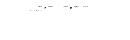
Figure 1: Gluon interactions do not change the helicity of the quarks

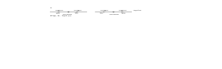
Figure 2: The mass terms change the helicity of the quarks

According to the theorem of E. Noether, there is one conserved current for each continuous parameter in the symmetry group. As the group $U(2)$ has four real parameters, one expects eight conserved currents. However, due to quantum effects, one of these currents is not conserved, as a result of which there are only seven conserved currents in the limit of vanishing quark masses,

$$L_{\mu}^{a} = \bar{q}_{L}\gamma_{\mu}\frac{\tau^{a}}{2}q_{L}\;,\;R_{\mu}^{a}=\bar{q}_{R}\gamma_{\mu}\frac{\tau^{a}}{2}q_{R}\;\ ;\;\;a=1,2,3$$

$$V_{\mu} = \bar{q}\gamma_{\mu}q\;\ ;\;\;q=\biggl{(}\begin{tabular}[]{c}$u$\\ $d$\end{tabular}\biggr{)}\;.$$ (2.23)

The world at

$$m_{u}=m_{d}=0$$

is called the chiral limit of QCD, and the above statements are summarized as: In the chiral limit, ${\cal L}_{\mathrm{QCD}}$ is symmetric under global $SU(2)_{L}\times SU(2)_{R}\times U(1)_{V}$ transformations. The corresponding 7 Noether currents (2.1) are conserved.

2.2 Symmetry of the ground state

It is useful to introduce in addition the vector and axial currents

$$V^{\mu a} = \bar{q}\gamma^{\mu}\frac{\tau^{a}}{2}q=L^{\mu a}+R^{\mu a}\;,\;$$

$$A^{\mu a} = \bar{q}\gamma^{\mu}\gamma_{5}\frac{\tau^{a}}{2}q=R^{\mu a}-L^{\mu a}\;\ ;\;\;a=1,2,3\;.$$

The corresponding 6 axial and vector charges $Q_{A,V}^{a}$ are conserved and commute with the hamiltonian $H_{0}=H_{\mathrm{QCD}}|_{m_{u}=m_{d}=0}$,

$$[H_{0},Q_{V}^{a}]=[H_{0},Q_{A}^{a}]=0\;\ ;\;\;a=1,2,3\;.$$ (2.24)

Consider now eigenstates of $H_{0}$,

$$H_{0}|\psi\rangle=E|\psi\rangle\;.$$

Then the states $Q_{A}^{a}|\psi\rangle\,\,{\mbox{and}}\,\,Q_{V}^{a}|\psi\rangle$ have the same energy $E$, but carry opposite parity. On the other hand, there is no trace [3] of such a symmetry in nature. The resolution of the paradox has been provided by Nambu and Lasinio back in 1960 [4]: whereas the vacuum is annihilated by the vector charges, it is not invariant under the action of the axial charges,

$$Q_{V}^{a}|0\rangle=0\;,\;Q_{A}^{a}|0\rangle\neq 0\;.$$ (2.25)

There are two important consequences of this assumption:

• The spectrum of $H_{0}$ contains three massless, pseudoscalar particles (Goldstone bosons (GB); Goldstone [5]). We will see more of this in the following section.

• The axial charges $Q_{A}^{a}$, acting on any state in the Hilbert space, generate Goldstone bosons,

  $$Q_{A}^{a}|\psi\rangle=|\psi,G_{1},\ldots,G_{N},\ldots\rangle\;.$$

  These are not one-particle states, and are therefore not listed in PDG, and there is therefore no contradiction anymore.

A theory with (2.24), (2.25) is called spontaneously broken: the symmetry of the hamiltonian is not the same as the symmetry of the ground state.

Where are the three massless, pseudoscalar states? The three pions $\pi^{\pm},\pi^{0}$ are the lightest hadrons. They are not massless, because the quark masses are not zero in the real world [6]:

$$m_{u} \simeq 5\,\mbox{MeV}\;,$$

$$m_{d} \simeq 9\,\mbox{MeV}\;.$$ (2.26)

In the following, we assume that the flavour symmetry of QCD is spontaneously broken to the diagonal subgroup,

$SU(2)_{L}\times SU(2)_{R}\rightarrow SU(2)_{V}$

and work out the consequences for the interactions between the Goldstone bosons.

Remark: Vafa and Witten [7] have shown that – modulo highly plausible assumptions – the vector symmetry $SU(2)_{V}$ is not spontaneously broken.

2.3 A remark on isospin symmetry

Even if the quarks are not massless, the QCD lagrangian has a residual symmetry at $m_{u}=m_{d}$: it is invariant under the transformations (2.20) with $V_{R}=V_{L}\in SU(2)$. This symmetry is called isospin symmetry. We know from textbooks that isospin symmetry violations in the strong interactions are small. On the other hand, according to (2.2), one has

$$m_{d}/m_{u}\simeq 1.8\;.$$ (2.27)

How can then isospin be a good symmetry if the quark masses differ so much? Consider the neutral and the charged pions: is it so that their masses differ by

$$(M_{\pi^{+}}^{2}-M_{\pi^{0}}^{2})/M_{\pi^{0}}^{2}\simeq\frac{m_{d}-m_{u}}{m_{d}+m_{u}}\simeq 0.3\,\,?$$

The answer is no: one has

$$M_{\pi^{+}}^{2}=(m_{u}+m_{d})B+\cdots\;,$$

$$M_{\pi^{0}}^{2}=(m_{u}+m_{d})B+\cdots\;,$$

where the ellipses denote higher order terms in the quark mass expansion. The neutral and the charged pion have the same leading term, the quark mass difference shows up only in the quadratic piece,

$$M_{\pi^{+}}^{2}-M_{\pi^{0}}^{2}=O[(m_{u}-m_{d})^{2}]\;.$$

The perturbation due to the quark masses can be written as

$$m_{u}\bar{u}u+m_{d}\bar{d}d = \frac{1}{2}(m_{u}+m_{d})(\bar{u}u+\bar{d}d)$$

$$+ \frac{1}{2}(m_{u}-m_{d})(\bar{u}u-\bar{d}d)\;.$$

Isospin is a good symmetry, not because $(m_{d}-m_{u})/(m_{d}+m_{u})$ is small, but because the matrix elements of the operator $\frac{1}{2}(m_{d}-m_{u})(\bar{u}u-\bar{d}d)$ are small with respect to the hadron masses. The bulk part in the pion mass difference is generated by electromagnetic interactions.

3 Goldstone bosons

In this section, I discuss the Goldstone theorem, illustrate it with several examples and consider the interaction of Goldstone bosons at low energy.

3.1 The Goldstone theorem

We consider a quantum field theory which has the following properties:

• There is a conserved current (i.e., an object that transforms as a four-vector under proper Lorentz transformations),

  $$A_{\mu}(x)\;\ ;\;\;\,\partial^{\mu}A_{\mu}=0.$$

• There is an operator $\Phi(x)$ such that

  $$\langle 0|[Q,\Phi]|0\rangle\neq 0\;\ ;\;\;Q=\int d^{3}xA_{0}(x^{0},\vec{x}).$$ (3.1)

Then the Goldstone theorem [5] applies:

1. There exists a massless particle in the theory,

   $$|\pi(\mathbf{p})\rangle\;,\;p^{2}=0\;.$$

2. The current $A_{\mu}$ couples to the massless state,

   $$\langle 0|A_{\mu}(0)|\pi(\mathbf{p})\rangle=ip_{\mu}F\neq 0\;.$$

From the condition (3.1), it is seen that the charge $Q$ does not annihilate the vacuum.

3.2 The free scalar field

We begin with a very simple example, the free, massless scalar field. The lagrangian is given by

$${\cal L}_{0} \!= \!\frac{1}{2}\partial_{\mu}\phi\partial^{\mu}\phi\;.$$

For the current $A_{\mu}$, we take

$$A_{\mu}\!=\!\partial_{\mu}\phi\;.$$

This current is conserved, because $\phi$ is a free field. Consider now $\Phi=\phi$. From the canonical commutation relations, it follows that the condition (3.1) is satisfied. Therefore, the Goldstone theorem applies. Indeed, we can easily check directly:

$$\bullet\,\,\phi\,\,\mbox{generates massless states}\;,$$

and

$$\bullet\,\,\langle 0|A_{\mu}(0)|\pi\rangle=-ip_{\mu}\neq 0\;.$$

3.3 The linear sigma model

We consider the linear sigma model ($L\sigma M\,\,$), because it allows one to illustrate many features of effective field theories. At the same time, it serves as a model with spontaneous symmetry breaking. The lagrangian is

$${\cal L}_{\sigma}=\frac{1}{2}\partial_{\mu}\vec{\phi}\cdot\,\partial^{\mu}\vec{\phi}-\frac{g}{4}(\vec{\phi}^{2}-v^{2})^{2}\;,$$ (3.2)

where $\vec{\phi}=(\phi^{0},\phi^{1},\phi^{2},\phi^{3})$ denotes four real fields, and $\vec{\phi}^{2}=\phi^{k}\phi^{k}$ [repeated indices are summed over in the absence of a summation symbol]. In the following, we assume that

$$v^{2}>0\;,$$

and discuss

1. the symmetry properties of ${\cal L}_{\sigma}$

2. spontaneous symmetry breakdown

3. Goldstone bosons

4. quantization

5. Goldstone boson scattering

Symmetry properties Here, we consider the classical theory and observe that ${\cal L}_{\sigma}$ is invariant under four-dimensional rotations of the vector $\vec{\phi}$,

$$\phi^{i}\rightarrow R^{ik}\phi^{k}\;,\;R\in O(4)\;.$$

The matrices $R$ can be parametrized in terms of six real parameters. Let us consider infinitesimal rotations

$$R=1+\varepsilon+O(\varepsilon^{2})\;.$$

Because $R$ is an orthogonal matrix, $\varepsilon$ is antisymmetric, $\varepsilon+\varepsilon^{T}=0$. Every real and antisymmetric four by four matrix can be expanded in terms of six generators,

$$\varepsilon=\sum_{i=1}^{3}\biggl{(}c_{i}\varepsilon_{V}^{i}+d_{i}\varepsilon_{A}^{i}\biggr{)}\;,$$

where $c_{i},d_{i}$ are 6 real parameters. The generators

satisfy the commutation relations

$[\varepsilon_{V}^{a},\varepsilon_{V}^{b}]=\varepsilon^{abc}\varepsilon_{V}^{c}\;,$

$[\varepsilon_{V}^{a},\varepsilon_{A}^{b}]=\varepsilon^{abc}\varepsilon_{A}^{c}\;,$

$[\varepsilon_{A}^{a},\varepsilon_{A}^{b}]=\varepsilon^{abc}\varepsilon_{V}^{c}\;,$

with $\varepsilon^{123}=1$, cycl. The linear combinations

$$Q_{L}^{a}=\frac{1}{2}(\varepsilon_{V}^{a}-\varepsilon_{A}^{a})\;,\;Q_{R}^{a}=\frac{1}{2}(\varepsilon_{V}^{a}+\varepsilon_{A}^{a})\;,$$

generate two commuting $SU(2)$ Lie-algebras (up to a factor $i$),

(3.5)

In other words, the lagrangian ${\cal L}_{\sigma}$ has a $SU(2)_{L}\times SU(2)_{R}$ symmetry. As a result of this, there are six conserved Noether currents, which we take to be

$$V_{\mu}^{a} = \varepsilon^{abc}\phi^{b}\partial_{\mu}\phi^{c}\;,$$

$$A_{\mu}^{a} = -\phi^{0}\stackrel{{\scriptstyle\leftrightarrow}}{{\partial}}_{\mu}\phi^{a}\;\ ;\;\;a=1,2,3\;.$$

Spontaneous symmetry breaking

The potential $V={g}(\vec{\phi}^{\,\,2}-v^{2})^{2}/4$ is extremal at $\phi=0$ and at $\vec{\phi}^{\,\,2}=v^{2}$. The latter configuration corresponds to a global minimum. The vector

$$\vec{\phi}_{G}=(v,\vec{0})\;,$$

which realizes this global minimum, is only invariant under the subgroup $H=O(3)$ (with generators $\varepsilon_{V}^{a}$), see figure 3 for the case where the symmetry group is $O(2)$. The number of generators that do not leave invariant $\vec{\phi}_{G}$ is $n_{G}-n_{H}=3$, where

$$n_{G}: \mbox{$\#$ of parameters in O(4)}\;,$$

$$n_{H}: \mbox{$\#$ of parameters in O(3)}\;.$$

Therefore, one expects three Goldstone bosons in the spectrum of the theory.

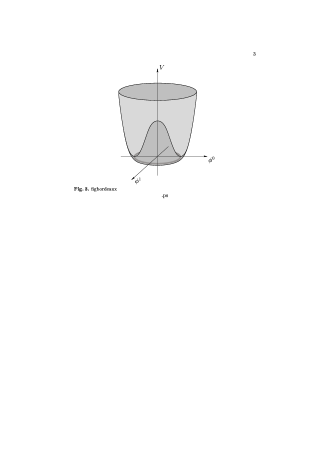
Figure 3: Potential for $O(2)$

Goldstone bosons

In order to identify the Goldstone bosons, we consider fluctuations around the configuration $\vec{\phi}_{G}$, and write

$$\vec{\phi}=(v+\varphi_{0},\vec{\pi})\;\ ;\;\;\vec{\pi}=(\pi^{1},\pi^{2},\pi^{3})\;,$$

where we have introduced the pion fields $\vec{\pi}$. In terms of the new fields, the lagrangian becomes

$${\cal L}_{\sigma} = \frac{1}{2}[\partial_{\mu}\varphi_{0}\partial^{\mu}\varphi_{0}-2gv^{2}\varphi_{0}^{2}]+\frac{1}{2}\partial_{\mu}\vec{\pi}\cdot\partial^{\mu}\vec{\pi}$$ (3.6)

$$-gv\varphi_{0}\,(\varphi_{0}^{2}+\vec{\pi}^{\,2})-\frac{g}{4}(\varphi_{0}^{2}+\vec{\pi}^{\,\,2})^{2}\;.$$

The kinetic term shows that there is indeed one massive field $\varphi_{0}$, with mass $m=\sqrt{2g}v$, together with three massless fields $\vec{\pi}$.

Quantization

One evaluates Green functions generated by the lagrangian (3.6) in the standard manner. At tree level, one has one massive and three massless fields, as in the classical theory. Evaluating loops, one finds that $\varphi_{0}$ picks up a vacuum expectation value at order $\hbar$. One shifts this field again, such that the new field has a vanishing one-point Green function, and finds that the remaining three particles stay massless also in the loop expansion.

Goldstone boson scattering

Finally, we consider GB scattering at tree level, with the lagrangian (3.6). In particular, we consider the process

$$\pi^{1}(p_{1})\pi^{2}(p_{2})\rightarrow\pi^{3}(p_{3})\pi^{4}(p_{4})\;,$$

where $\pi^{1}$ denotes the GB number one, etc. The relevant diagrams are displayed in Fig. 4.

Figure 4: Goldstone boson scattering with the lagrangian (3.6). Solid (dashed) lines stand for massless (massive) particles

The scattering matrix element has the structure

$$T^{kl;ij} = \delta^{ij}\delta^{kl}A(s,t,u)+\mbox{cycl.}\;,$$ (3.7)

$$s=(p_{1}+p_{2})^{2},t=(p_{3}-p_{1})^{2},u=(p_{4}-p_{1})^{2}\;.$$

(The Kronecker symbols occur, because the lagrangian is invariant under an $O(3)$ rotation of the pion fields $\vec{\pi})$. The invariant amplitude is

$$A(s,t,u)=\frac{4g^{2}v^{2}}{m^{2}-s}-2g\;.$$ (3.8)

At small momenta, the constant terms cancel out,

$$A(s,t,u)=\frac{s}{v^{2}}+O(s^{2})\;.$$ (3.9)

In other words, the interaction between the GB vanishes at zero momenta. The constant $v$ is related to the matrix elements of the axial current,

$$\langle 0|A_{\mu}^{a}(0)|\pi^{b}(p)\rangle=i\delta^{ab}vp_{\mu}\;.$$

3.4 QCD with two flavors

We now go back to the discussion of the Goldstone theorem in the framework of QCD. In section 2, we noted that the three axial currents $A_{\mu}^{a}$ are conserved in the case of vanishing quark masses. For the field $\Phi$ in (3.1), we choose $\Phi=\bar{q}\gamma_{5}\tau^{a}q$ (three fields, one for each a). Applying canonical commutation relations, one finds that

$$[Q_{A}^{a},\Phi^{b}]=-\delta^{ab}(\bar{u}u+\bar{d}d)\;\ ;\;\;a,b=1,2,3\;.$$

Provided that the vacuum expectation value of the quark bilinear is different from zero, the Goldstone theorem applies:

$$\langle 0|\bar{u}u|0\rangle\neq 0\Rightarrow{\mbox{3 Goldstone bosons}}\;.$$

(The vacuum expectation value of $\bar{u}u$ is equal to the one of $\bar{d}d$ by isospin symmetry.) Lattice calculations support the conjecture that $\langle 0|\bar{u}u|0\rangle$ is different from zero. Later in these lectures, we shall see that data on $K_{e4}$ decays do so as well.

How does one evaluate GB scattering in QCD? This is a very complicated affair: the QCD lagrangian contains quark and gluon fields, not pion fields. On the other hand, if QCD is spontaneously broken in the manner just discussed, the Goldstone theorem guarantees that the axial current can be used as an interpolating field for the pion [8]. Let us consider therefore the matrix element

$$G_{\mu}(p_{4},p_{3};p_{1})=\langle\pi(p_{3})\pi(p_{4}){\mbox{out}}|A_{\mu}(0)|\pi(p_{1})\rangle\;,$$ (3.10)

where I have suppressed all isospin indices. This matrix element has two parts: one, where the axial current generates a pion pole, and a second one, which is free from one-particle singularities, see Fig. 5.

Figure 5: Singular and non singular contributions to the matrix element (3.10) of the axial current. The wavy line denotes the axial current, the solid lines the pions

According to the LSZ reduction formula [9], the quantity $G_{\mu}$ has the structure

$$G_{\mu}=\frac{Fq_{\mu}}{q^{2}}T(p_{3},p_{4};p_{1})+R_{\mu}\;,$$ (3.11)

where $T$ denotes the elastic $\pi\pi$ scattering matrix element, and where $F$ is the pion decay constant,

$$\langle 0|A_{\mu}(0)|\pi(p)\rangle=ip_{\mu}F\;.$$

The remainder $R_{\mu}$ is non singular when $q^{\mu}=(p_{3}+p_{4}-p_{1})^{\mu}$ is sent to zero. We contract both sides in (3.11) with $q^{\mu}$. Because the axial current is conserved, the left-hand side vanishes, and therefore

$$FT(p_{3},p_{4};p_{1})+q^{\mu}R_{\mu}=0\;.$$

One concludes that the scattering matrix element vanishes at $q^{\mu}=0$ - this was easy to prove! We find again that the GB do not interact at vanishing momenta. One can even go further: as already mentioned in the introduction, Weinberg determined in 1966 [1] – using current algebra – the leading term of the $\pi\pi$ scattering amplitude in a systematic expansion of the momenta and of the pion mass.

4 Effective field theories

As we have just seen, it is possible to get a great deal of information about the interactions of GB in QCD without actually solving the theory. Effective field theories (EFT) provide the proper framework to perform detailed calculations in a systematic manner. EFT are valid in a restricted energy region, describing there an underlying theory that is valid on a wider energy scale. The situation for the Standard Model is illustrated in Fig. 6.

Figure 6: The Standard Model at various energy scales. At low energy, the effective theory is formulated in terms of physical fields

Effective field theories are in particular useful, when a full calculation is not yet possible, as is the case with the Standard Model at low energies. One sets up an EFT with the same symmetry properties – in case of the Standard Model, this effective theory is called Chiral perturbation theory. A second possibility for the use of EFT occurs in case that the calculations can be done in the underlying theory, but are very complicated. An example is provided by the calculation of bound states in the framework of QED, which can be performed, in principle, at any desired order by use of the Bethe-Salpeter equations. On the other hand, as Caswell and Lepage have shown [10], the use of EFT makes life very much simpler also in this case, because the electrons and positrons are moving very non-relativistically in the atoms, and a relativistic calculation is not really needed. Further applications concern the case where the underlying theory is not known – one builds the effective theory in terms of the light fields and attempts to determine from experiment the unknown coupling constants that occur in there.

In the following, I discuss the low-energy EFT for the $L\sigma M\,\,$and for QCD.

4.1 Linear sigma model at low energy

We have seen in the last section that the $O(4)$ version of the $L\sigma M\,\,$in its broken phase develops three Goldstone bosons, which interact weekly at low energy (we have proven this at tree level only).

In the following, we construct an effective theory that contains only pions and their interactions - the sigma particle is removed from the theory. This EFT is constructed in such a manner that the Green functions with pion fields, evaluated in the $L\sigma M\,\,$at low energies, are recovered by the EFT. How can this be achieved?

As a first step, one constructs an EFT which reproduces all tree graphs at low energies, to any order in the low-energy expansion: as is seen from the explicit expression (3.8), the scattering matrix element contains arbitrarily high powers in the momenta even at tree level. The procedure to construct the effective lagrangian is described in detail in the article by Nyffeler and Schenk [11] - I do not repeat the argument here and refer the interested reader instead to this work. The result can be written in various equivalent forms. Here, I use

$${\cal L}_{\mathrm{eff}}^{\sigma} = {\cal L}_{2}^{\sigma}+{\cal L}_{4}^{\sigma}+\cdots\;.$$

The lagrangians ${\cal L}_{n}^{\sigma}$ contain $n$ derivatives of the pion fields. These derivatives become momenta in Fourier space: the effective lagrangian provides a momentum expansion of the amplitudes. Explicitly, one has for the leading term

$${\cal L}_{2}^{\sigma} = \frac{v^{2}}{4}\langle\partial_{\mu}U\partial^{\mu}U^{\dagger}\rangle\;,$$ (4.1)

where $U$ is a $2\times 2$ unitary matrix,

$$U = \sigma\cdot{\bf 1}_{2\times 2}+\frac{i}{v}\tau^{k}\pi^{k}\,\;\ ;\;\;\,\sigma^{2}+\frac{\vec{\pi}^{2}}{v^{2}}=1\;,\vec{\pi}=(\pi^{1},\pi^{2},\pi^{3})\;.$$

The symbol $\langle A\rangle$ denotes the trace of the matrix $A$, and $\tau^{k}$ are the Pauli matrices. In order to illustrate the structure of this lagrangian, we expand it in terms of the pion fields:

$${\cal L}_{2}^{\sigma}=\frac{1}{2}\partial_{\mu}{\vec{\pi}}\cdot\partial^{\mu}{\vec{\pi}}+\frac{1}{8v^{2}}\partial_{\mu}{\vec{\pi}}^{2}\partial^{\mu}{\vec{\pi}}^{2}+O({\vec{\pi}}^{6})\;.$$

The lagrangians ${\cal L}_{4,6,8\ldots}^{\sigma}$ have a similar structure [11].

Comments

• Only pions occur in the effective theory, the heavy particle has disappeared.

• It is easy to calculate the $\pi\pi$ scattering amplitude at tree level with ${\cal L}_{2}^{\sigma}$ - only one diagram remains to be calculated. The result is identical to the first term on the right-hand side of (3.9). The higher order terms in the expansion of the amplitude (3.8) are generated by the tree graphs of ${\cal L}_{4,6,..}^{\sigma}$.

• The mass of the sigma particle is given by $m=\sqrt{2g}v$. As a result of this, the interactions disappear formally in the large-mass limit.

• Where has the $O(4)$ symmetry of the $L\sigma M\,\,$gone? ${\cal L}_{2}^{\sigma}$ is invariant under

  $$U\rightarrow V_{R}UV_{L}^{\dagger};\,\,V_{R,L}\in SU(2)\;.$$

  Therefore, the effective theory has an $SU(2)_{R}\times SU(2)_{L}$ symmetry, as the original theory.

• How is the spontaneously broken symmetry realized?

  $U_{G}={\bf 1}_{2\times 2}$ is the ground state. It is only invariant under

  $$U_{G}\rightarrow VU_{G}V^{\dagger}\;.$$

Therefore, the theory is spontaneously broken,

$$SU(2)_{R}\times SU(2)_{L}\Rightarrow SU(2)_{V}\;,$$

and generates three Goldstone bosons.

The lagrangian ${\cal L}_{\mathrm{eff}}^{\sigma}$ reproduces the tree graphs of the $L\sigma M\,\,$- how about loops? Indeed, one may calculate the scattering amplitudes in the framework of the $L\sigma M\,\,$to any order in the loop expansion, perform a low-energy expansion of the result, and finally construct an effective theory that reproduces the result of this calculation, order by order in the low-energy expansion. The procedure is carried out to one loop in [12, 11].

4.2 QCD at low energy

The effective theory of QCD is formulated in terms of asymptotic pion fields. As is the case for the $L\sigma M\,\,$, the effective theory consists of an infinite number of terms, with more and more derivatives [13, 12]:

$${\cal L}_{\mathrm{eff}}={\cal L}_{2}+{\cal L}_{4}+{\cal L}_{6}+\cdots\;.$$ (4.2)

All that goes into the construction of ${\cal L}_{\mathrm{eff}}$ are symmetry properties of QCD. The result for the leading term is

$${\cal L}_{2} = \frac{F^{2}}{4}\langle\partial_{\mu}U\partial^{\mu}U^{\dagger}+2B{\cal M}(U+U^{\dagger})\rangle\;,$$ (4.3)

where the field $U$ is the same as above, and where

$${\cal M}=\biggl{(}\begin{tabular}[]{ll}$m_{u}$&0\\ 0&$m_{d}$\end{tabular}\biggr{)}$$ (4.6)

contains the quark masses $m_{u},m_{d}$. A glance at (4.1) shows that, at $m_{u}=m_{d}=0$, the leading order lagrangians in the $L\sigma M\,\,$and in QCD agree, provided that one sets $v=F$. The leading term (4.3) contains the two constants $F$ and $B$ which are related to the pion decay constant and to the quark condensate, respectively [12],

$$\langle 0|A_{\mu}^{a}(0)|\pi^{b}(p)\rangle = ip_{\mu}F\delta^{ab}\;,$$

$$\langle 0|\bar{u}u|0\rangle_{|_{m_{u}=m_{d}=0}} = -F^{2}B\;.$$

We have made a very big step: we have replaced the QCD lagrangian ${\cal L}_{\mathrm{QCD}}$ by the effective lagrangian ${\cal L}_{\mathrm{eff}}$. This transition may be visualized in terms of Feynman graphs: in Fig. 7 is displayed one of the infinitely many graphs that contribute to $\pi\pi$ scattering in QCD, and which are all equally important. On the other hand, in the effective theory, only the two graphs displayed in Fig. 8 contribute at leading order. In the figure, the symbol $M^{2}$ stands for the combination

$$M^{2}=(m_{u}+m_{d})B$$ (4.7)

which finally counts in ${\cal L}_{2}$, see below. The crucial point to observe is the fact that the transition

${\cal L}_{\mathrm{QCD}}\Rightarrow{\cal L}_{\mathrm{eff}}$

is a non perturbative phenomenon. It is very different from the construction of the effective theory for the linear sigma model, where the loop expansion in the original theory does make sense, and where the low-energy representation can be worked out order by order in the loop expansion.

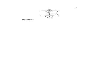
Figure 7: $\pi\pi$ scattering in QCD. Displayed is one of the infinitely many graphs that contribute in QCD, and which are all equally important

Figure 8: Evaluating the $\pi\pi$ scattering amplitude with the effective lagrangian ${\cal L}_{2}$ in (4.3). Only the two graphs displayed contribute at leading order. The symbol $M^{2}$ is defined in (4.7)

I have provided

1. no proof that ${\cal L}_{2}$ is the correct leading order lagrangian.

2. no discussion of the group theoretical background (realization of the group $SU_{R}(2)\times SU_{L}(2)$ on curved manifolds).

For these issues, I refer the interested reader to earlier Schladming lectures by Leutwyler [14], Manohar[15] and Ecker[16]. Leutwyler has proven in [17] that the above lagrangian does reproduce the Green functions of QCD at low energy, see also below.

5 Calculations with ${\cal L}_{\mathrm{eff}}$

In the last section, we have displayed the effective lagrangian that allows one to evaluate masses, form factors and scattering matrix elements in QCD at low energy. The results are valid at small values of the quark masses and of the momenta. In this section, I illustrate the procedure with several examples.

5.1 Leading terms

Evaluating matrix elements at tree level with the effective lagrangian (4.3) generates the leading term in the low-energy expansion, see later for a precise meaning of this terminology.

Pion masses

Consider the kinetic term in ${\cal L}_{2}$,

$${\cal L}_{2} = \frac{1}{2}[\partial_{\mu}{\vec{\pi}}\cdot\,\partial^{\mu}{\vec{\pi}}-M^{2}{\vec{\pi}}^{2}]+O({\vec{\pi}}^{4})\;.$$

We conclude that the three pions have the same mass in this approximation,

$$M_{\pi^{\pm}}^{2}=M_{\pi^{0}}^{2}=M^{2}\;.$$ (5.1)

Remark: We denote by $M_{\pi^{\pm}}$ and $M_{\pi^{0}}$ the charged and neutral pion mass, respectively. The symbol $M_{\pi}$ stands for the pion mass in the isospin symmetry limit, whereas $M^{2}$ is the first term in the quark mass expansion of the charged and neutral pion (mass)².

$\pi\pi$ scattering

The terms of order $\vec{\pi}^{4}$ in ${\cal L}_{2}$ generate the leading term in the $\pi\pi$ scattering amplitude,

$${\cal L}_{2} = \mbox{kinetic term}\,+\,\frac{1}{8F^{2}}[\partial_{\mu}{\vec{\pi}}^{2}\partial^{\mu}{\vec{\pi}}^{2}-M^{2}{\vec{\pi}}^{4}]+O({\vec{\pi}}^{6})\;.$$

The couplings are

$$\frac{1}{F^{2}}\,\,\mbox{and}\,\,\frac{M^{2}}{F^{2}}\;.$$

In other words, the mass $M$ is also a coupling! Figure 8 displays the two diagrams that one has to evaluate in this case.

a) $\pi^{+}\pi^{-}\rightarrow\pi^{0}\pi^{0}$

The scattering matrix element is

$$T = \frac{M^{2}-s}{F^{2}}+O(p^{4})\;\ ;\;\;s=(p_{1}+p_{2})^{2}\;.$$

This result agrees with (1.1), up to the replacement $(M,F)$$\rightarrow(M_{\pi},F_{\pi})$, which is a higher order effect, included in the symbol $O(p^{4})$.

b) $\pi^{a}\pi^{b}\rightarrow\pi^{c}\pi^{d}$

The structure of the matrix element in the general case is displayed in (3.7). The invariant amplitude $A(s,t,u)$ becomes

$$A(s,t,u) = \frac{s-M^{2}}{F^{2}}+O(p^{4})\;.$$ (5.2)

c) Isospin amplitudes

For later use, we introduce here the isospin amplitudes

$$T^{I=0} = 3A(s,t,u)+A(t,u,s)+A(u,s,t)\;,$$

$$T^{I=1} = A(t,u,s)-A(u,s,t)\;,$$

$$T^{I=2} = A(t,u,s)+A(u,s,t)\;.$$

5.2 Higher order trees

Evaluating tree-level graphs with ${\cal L}_{2}$ generates the leading terms of the quantities in question. How about the contributions from ${\cal L}_{4}$? It contains e.g. terms with four derivatives, like

$${\cal L}_{4}=d_{1}\langle\partial_{\mu}U\partial^{\mu}U^{\dagger}\rangle^{2}+\cdots\;.$$

What is the effect of this term? From

$$\langle\partial_{\mu}U\partial^{\mu}U^{\dagger}\rangle^{2}=\frac{4}{F^{4}}(\partial_{\mu}{\vec{\pi}}\cdot\,\partial^{\mu}{\vec{\pi}})^{2}+\cdots\;,$$

we conclude that ${\cal L}_{4}$ also contributes to elastic $\pi\pi$ scattering. Since four derivatives are involved, there will be four powers of the momenta. Indeed, at tree level, ${\cal L}_{4}$ contributes with

$$\delta A(s,t,u)=\frac{8d_{1}}{F^{4}}(s-2M^{2})^{2}+\cdots\;.$$ (5.3)

This term is of order $p^{4}$ for small momenta. One can perform the expansion in a systematic manner - there are only a limited number of terms at order $p^{4}$ [12]:

$${\cal L}_{4} = \sum_{i=1}^{7}l_{i}P_{i}\;,$$

$$P_{1} = \frac{1}{4}\langle\partial_{\mu}U\partial^{\mu}U^{\dagger}\rangle^{2}\;,\;P_{2}=\frac{1}{4}\langle\partial_{\mu}U\partial_{\nu}U^{\dagger}\rangle\langle\partial^{\mu}U\partial^{\nu}U^{\dagger}\rangle\;,$$

$$P_{3} = \frac{1}{16}\langle 2B{\cal M}(U+U^{\dagger})\rangle^{2}\;,\;P_{7}=-\frac{1}{16}\langle 2B{\cal M}(U-U^{\dagger})\rangle^{2}\;.$$

$P_{4,5,6}$ do not contribute to the $\pi\pi$ scattering amplitude. Why is knowledge of ${\cal L}_{4}$ useful? Suppose that the LECs $l_{i}$ are known $\Rightarrow$ low-energy amplitudes are parametrized in terms of 7 parameters $\Rightarrow$ all other amplitudes fixed in terms of these parameters at this order in the low-energy expansion.

Comments

• Chiral symmetry and $C,P,T$ invariance have been used to determine ${\cal L}_{4}$. For example,

  $$\langle\partial_{\mu}U\partial^{\mu}U^{\dagger}\rangle^{2}$$

  is invariant under $U\rightarrow V_{R}UV_{L}^{\dagger}\;,\;V_{I}\in SU(2)\;.$

• The low-energy constants $l_{i}$ (LECs) are not fixed by symmetry arguments.

• The operators $P_{1,2,3,7}$ contribute to the following processes:

  (5.7)

Example

Taking into account the contributions from ${\cal L}_{4}$, the pion masses read at tree level

$$M_{\pi^{\pm}}^{2} = M^{2}+\frac{2l_{3}}{F^{2}}M^{4}\;,$$

$$M_{\pi^{0}}^{2} = M_{\pi^{\pm}}^{2}-\frac{2B^{2}}{F^{2}}(m_{d}-m_{u})^{2}l_{7}\;.$$ (5.8)

5.3 Loops

Scattering amplitudes, evaluated with

$${\cal L}_{2}+{\cal L}_{4}$$

at tree level, are still real. To be in accord with optical theorem, one needs to evaluate loops. This guarantees that unitarity is satisfied order by order in the low-energy expansion, like in any standard loop expansion in QFT. We illustrate the evaluation of loops in the case of the pion mass.

Pion mass

To evaluate the pion mass in the isospin symmetry limit $m_{u}=m_{d}$, we consider the connected two-point function

$$\delta^{ab}\triangle_{c}(p)=i\int d^{4}x\,e^{ipx}\langle 0|T\phi^{a}(x)\phi^{b}(0)|0\rangle_{c}\;.$$ (5.9)

Figure 9: Tree and tadpole contribution from ${\cal L}_{2}$ to the two-point function (5.9)

Taking into account the tree and tadpole contributions displayed in Fig. 9, we find that

$$\triangle_{c}(p)=\frac{Z}{M_{p}^{2}-p^{2}}\;,$$

where

$$M_{p}^{2} = M^{2}+\frac{M^{2}I}{2F^{2}}\;,\;I=\int\frac{d^{4}l}{i(2\pi)^{4}}\frac{1}{M^{2}-l^{2}}\;.$$

The tadpole integral $I$ is quadratically divergent. A standard method to cope with this situation is to perform the integral in $d$ dimensions,

$$I\rightarrow \int\frac{d^{d}l}{i(2\pi)^{d}}\frac{1}{M^{2}-l^{2}}=\frac{M^{d-2}}{(4\pi)^{d/2}}\Gamma(1-d/2)\;.$$

The result is now finite at $d\,\neq 2,4,6\ldots$, whereas it is still still divergent at $d=4:$

$${M^{2}I}\rightarrow\frac{M^{4}}{8\pi^{2}}\frac{1}{d-4}\;,\;d\rightarrow 4\;.$$

There is also a tree contribution from ${\cal L}_{4}$, see (5.2),

$$\delta M_{p}^{2}=\frac{2l_{3}}{F^{2}}M^{4}\;.$$

If we tune $l_{3}$ to diverge as $d\rightarrow 4$ as well, we may cancel the divergence in the mass:

$$l_{3}\rightarrow-\frac{1}{32\pi^{2}}\frac{1}{d-4}+\mbox{finite}\;,\;d\rightarrow 4$$

The physical pion mass at $m_{u}=m_{d}$ finally becomes

$$M_{\pi}^{2}=M^{2}-\frac{M^{4}}{32\pi^{2}F^{2}}\bar{l}_{3}+O(M^{6})\;.$$ (5.10)

The quantity ${\bar{l}}_{3}$ contains the finite parts from $l_{3}$ and from the tadpole integral $I$ [12].

Comments

• The required counterterm to cancel the divergence stems from ${\cal L}_{4}$. The divergences cannot be canceled by tuning parameters in ${\cal L}_{2}$: this is a typical feature of a non-renormalizable theory.

• Non-renormalizability does not mean non-calculability: the effective theory of QCD allows one to calculate all quantities perfectly well. The only disadvantage is the increasing number of low-energy coupling constants that one is faced with while incorporating higher order terms in the expansion.

• The contribution from the tadpole is suppressed, it is of order $M^{4}$, not of order $M^{2}$.

5.4 Renormalization made systematic

Similar divergences occur in other amplitudes, like $\pi\pi\rightarrow\pi\pi$, when loops are calculated. These divergences can all be canceled by tuning the $l_{i}$ in the lagrangian with four derivatives. The final prescription for the evaluation of the Green functions at order $p^{4}$ reads as follows: the effective lagrangian is

$${\cal L}_{\mathrm{eff}}={\cal L}_{2}+{\cal L}_{4}+{\cal L}_{6}+\cdots\;,$$

where ${\cal L}_{2}$ is given in (4.3), and

$${\cal L}_{4} = \sum_{i=1}^{7}l_{i}P_{i}\;,\;{\cal L}_{6}=\sum_{i=1}^{53}c_{i}Q_{i}\;.$$

The polynomials $P_{i}\,(Q_{i})$ and the divergent parts in the LECs $l_{i}\,(c_{i})$ have been determined in [12]  ([18]). At order $p^{6}$, there are in addition so called parity odd terms, that come with an epsilon tensor [19]. Further, some of the polynomials $P_{i},Q_{i}$ vanish in the absence of external fields. I refer the reader to [18] for a guided tour through ${\cal L}_{6}$.

The Green functions are calculated as follows:

leading terms:     trees with ${\cal L}_{2}$

$$\mbox{next-to-leading terms: \hskip 5.69054pt}\biggl{\{}\begin{tabular}[]{ll}trees with&${\cal L}_{4}$\\ one loop with&${\cal L}_{2}$\end{tabular}$$ (5.13)

$$\mbox{next-to-next-to-leading terms:\hskip 5.69054pt}\biggl{\{}\begin{tabular}[]{ll}trees with&${\cal L}_{6}$\\ one loop with&${\cal L}_{4}$\\ two loops with&${\cal L}_{2}$\\ \end{tabular}$$ (5.17)

Comments

1. Next-to-leading terms are suppressed by $p^{2}$ with respect to the leading term, the next-to-next-to leading terms by $p^{4}$, etc.

2. The finite parts of the low-energy constants $l_{i},c_{i}$ are not fixed by symmetry considerations. On the other hand, they are calculable in principle in QCD. We are witnessing a transition period, where one starts to be able to evaluate the LECs in the framework of QCD - see [20] for recent examples.

3. Meanwhile, until the transition period is over, one takes LECs from data, from sum rules etc.

4. We will comment in the final section about the introduction of additional fundamental fields in the effective lagrangian.

6 Pion-pion scattering

In this section, I consider in some detail the evaluation of the elastic $\pi\pi$ scattering amplitude in the low-energy region at order $p^{6}$. The motivation for investigating this reaction in great detail includes the following points:

1. It is possible to make precise theoretical predictions.

2. Some of the threshold amplitudes are sensitive to the mechanism of spontaneous chiral symmetry breaking.

3. There are new experimental activities:

   BNL-865 at Brookhaven	$K_{e4}$ decays	[22]
   NA48 at CERN	$K_{e4}$ decays	[23]
   KLOE at DAFNE	$K_{e4}$ decays	[24]
   DIRAC at CERN	$\pi^{+}\pi^{-}$ atom	[25]

4. The analysis of the $P$-wave amplitude in elastic $\pi\pi$ scattering provides very useful information for the evaluation of the anomalous magnetic moment of the muon [26].

Why do the so called $K_{e4}$ decays

$$K^{+} \rightarrow\pi^{+}\pi^{-}e^{+}\nu_{e}\;,$$

$$K^{+} \rightarrow\pi^{0}\pi^{0}e^{+}\nu_{e}\;,$$

$$K^{0} \rightarrow\pi^{0}\pi^{-}e^{+}\nu_{e}\;,$$

and their charge conjugate modes provide information on $\pi\pi$ scattering?

First explanation

The emerging pions in the decay products interact with each other (final state interaction). The decay width is therefore sensitive to this interaction.

Second explanation (more learned)

The decay matrix element is described by form factors. One may perform a partial wave analysis of these - the partial wave amplitudes then carry the phases of the $\pi\pi$ interaction (Watson’s final state theorem). In the decay, one measures interference terms between the various partial waves. The decay of the charged kaon into a charged pion pair plus leptons turns out to be sensitive to

$$\delta_{l=0}^{I=0}(E_{\pi\pi})-\delta_{1}^{1}(E_{\pi\pi})\;,$$

where $E_{\pi\pi}$ denotes the centre-of-mass energy of the pion pair. The investigation of $\pi^{+}\pi^{-}$ atoms (Pionium) is of interest for the following reason. The atom is formed by electromagnetic interactions. It is not stable - the ground state, e.g., has various decay channels,

$$A_{\pi^{+}\pi^{-}}\rightarrow\pi^{0}\pi^{0},\gamma\gamma,\pi^{0}\pi^{0}\gamma\gamma,\ldots\;.$$

The decay into the neutral pion pair depends on the strength of the strong interactions [27, 28],

$$\Gamma=\frac{2}{9}\alpha^{3}p^{*}|a_{0}^{0}-a_{0}^{2}|^{2}(1+\delta)\;,$$ (6.1)

where $a_{0}^{0}$ denotes the $I=0$ $S$-wave scattering length $a_{l=0}^{I=0}$, and $p^{*}$ is the modulus of the centre-of-mass momentum of the neutral pions in the rest system of the decaying atom. Further, $\alpha\simeq 1/137$ is the fine structure constant of QED. The decay width into a photon pair is suppressed by the factor $\alpha^{3/2}$ with respect to the $\pi^{0}\pi^{0}$ channel. The correction $\delta$ is also known [28],

$$\delta=0.058\pm 0.012\;.$$

A measurement of the lifetime of the ground state therefore amounts to a measurement of the combination $|a_{0}^{0}-a_{0}^{2}|$.

6.1 Chiral expansion of the $\pi\pi$ amplitude

The chiral expansion of the invariant scattering amplitude $A(s,t,u)$ is performed in the manner discussed in the previous section and has the structure

$$A(s,t,u) = A_{2}+A_{4}+A_{6}+\cdots\;,$$

where $A_{2n}$ is of order $p^{2n}$.

Leading order

The leading order result is given in (5.2). For the $I=0$ $S$-wave scattering length, one obtains from that expression

$$a_{0}^{0}=\frac{7M^{2}}{32\pi F^{2}}=0.16\;.$$ (6.2)

In the numerical evaluation, I have replaced $M$ and $F$ by $M_{\pi^{\pm}}$ = 139.57 MeV and by $F_{\pi}=92.4$ MeV, respectively (the replacements amount to taking into account some of the higher order effects in the calculation of the scattering amplitude). The data on $K_{e4}$ decays collected in the seventies gave [29]

$$a_{0}^{0}=0.26\pm 0.05\qquad\mbox{[from 30'000 $K_{e4}$ decays]}\;.$$

The question was – for many years – whether this indicates a failure of the chiral prediction (6.2). Indeed, if the condensate $\langle 0|\bar{u}u|0\rangle$ is small or vanishing, one can understand a large value of the scattering length. This is the main idea of the so-called generalized chiral perturbation theory, which was much discussed at the end of the last millennium [30]. In order to decide the issue, one needs more precise data and a more precise calculation. Both is available in our days, as we will show below.

Next-to-leading order

One evaluates one-loop graphs with ${\cal L}_{2}$ and tree-graphs with ${\cal L}_{4}$. Some of these are displayed in Fig. 10.

Figure 10: One-loop graphs in elastic $\pi\pi$ scattering. The filled squares denote contributions from ${\cal L}_{4}$

The result can be written in the form

$$A_{4} = a_{1}M_{\pi}^{4}+a_{2}M_{\pi}^{2}s+a_{3}s^{2}+a_{4}(t-u)^{2}$$

$$+F(s)+G(s,t)+G(s,u)\;.$$

We note the following:

1. The amplitude $A_{4}$ carries four powers of momenta

2. $F,G$ denote loop functions. They generate the imaginary parts which are required by unitarity at order $p^{4}$. Example:

   $$F(s) = \frac{1}{2F_{\pi}^{4}}(s^{2}-M_{\pi}^{4})\bar{J}(s)\;,$$

   $$\bar{J}(s) = \frac{1}{16\pi^{2}}\biggl{\{}\sigma\log{\frac{1-\sigma}{1+\sigma}}+2+i\pi\sigma\biggr{\}}\;,$$

   $$\sigma = (1-{4M_{\pi}^{2}}/{s})^{1/2}\;\ ;\;\;s>4M_{\pi}^{2}\;.$$

   The function $\bar{J}(s)$ is analytic in the complex $s$-plane, cut along the real axis for $s\geq 4M_{\pi}^{2}$.

1. $a_{i}$ contain the low-energy constants $\bar{l}_{1,2,3,4}$ from ${\cal L}_{4}$. For example, the $I=0$ $S$-wave scattering length now reads

   $$a_{0}^{0} = \frac{7}{32\pi}\frac{M_{\pi}^{2}}{F_{\pi}^{2}}\biggl{\{}1+\varepsilon+O(M_{\pi}^{4})\biggr{\}}\;,$$

   $$\varepsilon = \frac{5}{84\pi^{2}}\frac{M_{\pi}^{2}}{F_{\pi}^{2}}\biggl{(}\bar{l}_{1}+2\bar{l}_{2}-\frac{3}{8}\bar{l}_{3}+\frac{21}{10}\bar{l}_{4}+\frac{21}{8}\biggr{)}\;.$$

2. the LECs $\bar{l}_{i}$ contain so-called chiral logarithms:

   $$\bar{l}_{i}\rightarrow-\log{M_{\pi}^{2}}\;,\;M_{\pi}\rightarrow 0\;,$$

   which generate large corrections,

$$a_{0}^{0} = \frac{7M_{\pi}^{2}}{32\pi F_{\pi}^{2}}\biggl{\{}1-\underbrace{\frac{9}{32\pi^{2}}\frac{M_{\pi}^{2}}{F_{\pi}^{2}}\log{M_{\pi}^{2}/\mu^{2}}}_{\chi\mbox{logarithm}}+\cdots\biggr{\}}\;.$$

The $\chi$ logarithms generate a $25\%$ correction at $\mu=1$ GeV.

Next-to-next-to leading order

In order to evaluate $A_{6}$, one needs to perform a two-loop calculation with ${\cal L}_{2}$, one-loop with ${\cal L}_{4}$ and trees with ${\cal L}_{6}$. A few of the two-loop graphs are displayed in Fig. 11.

Figure 11: Two-loop graphs in elastic $\pi\pi$ scattering

It turns out that all graphs can be evaluated in closed form [31]! The structure of $A_{6}$ is as follows:

$$A_{6} =$$ loop functions

$$+b_{1}M_{\pi}^{6}+b_{2}M_{\pi}^{4}s+b_{3}M_{\pi}^{2}s^{2}+b_{4}M_{\pi}^{2}(t-u)^{2}+b_{5}s^{3}+b_{6}s(t-u)^{2}\;.$$

The calculation determines $b_{1},\ldots,b_{6}$ in terms of the LECs at order $p^{4}$ and $p^{6}$ [31]. Obviously, one is faced with a problem here: one needs to determine the LECs before a precise prediction of the scattering lengths can be performed.

6.2 Type A,B LECs

One encounters the following LECs in the $\pi\pi$ amplitude up to and including terms of order $p^{6}$:

$\bar{l}_{1},\bar{l}_{2},\bar{l}_{3},\bar{l}_{4}$	:   ${\cal L}_{4}$
$\bar{r}_{1},....,\bar{r}_{6}$	:   ${\cal L}_{6}$

They come in two categories [32]:

1. Terms that survive in the chiral limit:

$\bar{l}_{1},\bar{l}_{2},\bar{r}_{5},\bar{r}_{6}$   type A

These LECs show up in momentum dependence of the $\pi\pi$ amplitude, and may therefore be determined phenomenologically.

2. Symmetry breaking terms:

$\bar{l}_{3},\bar{l}_{4},\bar{r}_{1},\bar{r}_{2},\bar{r}_{3},\bar{r}_{4}$   type B

These LECs specify the quark mass dependence of the amplitude. The $\pi\pi$ scattering amplitude cannot provide information on type B LECs, because one cannot vary the quark mass in experiments.

We discuss in the following section how these LECs can be determined, and what the result for the scattering lengths finally is.

7 Roy equations and threshold parameters

Roy equations allow one to determine type A LECs and to pin down the $\pi\pi$ scattering amplitude in the low-energy region with high precision. It is useful to discuss Roy equations in two steps. In the first step, no relation to chiral symmetry is used - the only ingredients are analyticity, unitarity, crossing symmetry, data above 800 MeV and Regge behaviour beyond 2 GeV. In a second step, one merges the representation of the amplitude with the chiral representation discussed in the previous section.

7.1 $\pi\pi\rightarrow\pi\pi$: Roy I

Analyticity, crossing symmetry and the Froissart bound lead to dispersion relations for the partial waves of the $\pi\pi$ scattering amplitude. As has been shown by Roy [33], the imaginary part of the partial waves is needed only in the physical region. These dispersion relations read

$$t_{\ell}^{I}(s)=k_{\ell}^{I}(s)+\sum_{I^{\prime}=0}^{2}\sum_{\ell^{\prime}=0}^{\infty}\int_{4M_{\pi}^{2}}^{\infty}ds^{\prime}\,K_{\ell\ell^{\prime}}^{II^{\prime}}(s,s^{\prime})\,\mbox{Im}\,t_{\ell^{\prime}}^{I^{\prime}}(s^{\prime})\;,$$

where $\ell(I)$ denotes the angular momentum (isospin) of the partial wave. The subtraction term $k^{I}_{\ell}(s)$ contains the scattering lengths $a_{0}^{0},a_{0}^{2}$, and the kernels $K_{\ell\ell^{\prime}}^{II^{\prime}}(s,s^{\prime})$ are explicitly known functions of $s$ and of $s^{\prime}$. At low energy, only $S$- and $P$- waves matter, and the contributions from the remaining waves may be expanded in a Taylor series. Unitarity expresses the imaginary parts of the partial waves in terms of the real parts (in the elastic region) – the above dispersion relations then become (singular) integral equations for the two $S$- and for the $P$-wave. These may be solved numerically [34, 36]. In [36], it has been shown that the two $S$-wave scattering lengths $a_{0}^{0},a_{0}^{2}$ are the essential parameters. Once these are fixed, experimental data (above 800 MeV) plus Regge behaviour above 2 GeV determine the amplitude in the low energy region to within rather small uncertainties. Figure 12 displays the universal band in the $a_{0}^{0}-a_{0}^{2}$ plane, for which solutions may be found. An example solution for the three waves is displayed in Fig. 13.

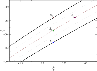
Figure 12: The universal band in the $a_{0}^{0}-a_{0}^{2}$ plane. For each point in this band, a unique solution to the Roy equations can be constructed

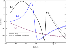
Figure 13: Example of a solution to the Roy equations. Displayed are the real parts of the partial waves, as a function of the centre-of-mass energy of the pions

7.2 $\pi\pi\rightarrow\pi\pi$: Roy II

In the previous subsection, no reference to ChPT was made. We now invoke this information: one requires that the $\chi$ amplitude agrees with phenomenological amplitude below the threshold region. Subtractions and matching are performed in such a manner that $\chi$ logarithms are suppressed. This procedure allows one to determine the type A LECs listed in subsection 6.2. Type B LECs are determined form other sources:

(7.4)

We have now arrived at solutions to the Roy equations that agree with the chiral amplitude at low energy. In other words, the three lowest partial waves below 800 MeV are fixed. The scattering lengths of the partial waves with $\ell\geq 1$, as well as the effective ranges (also those of the $S$-waves) can be expressed in terms of sum rules over the imaginary parts [37]. In Fig. 14 is displayed the resulting $P$-wave phase shift. This allows one to pin down the electromagnetic form factor of the pion with high precision [26].

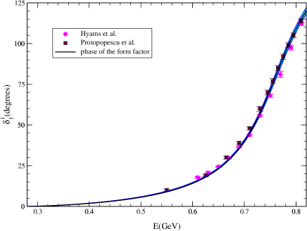
Figure 14: The $P$-wave from the Roy analysis

This form factor plays a very important role in the evaluation of the anomalous magnetic moment of the muon, see Marc Knecht’s lectures at this school.

Finally, we come to the two $S$-wave scattering lengths, which are now also fixed [38, 32],

$$a_{0}^{0} = 0.220\pm 0.005\;,$$

$$a_{0}^{0}-a_{0}^{2} = 0.265\pm 0.004\;.$$

I refer the reader to [32] for scattering lengths and effective ranges of other waves. The above result also provides [28] a precise prediction for the lifetime of Pionium in the ground state via (6.1),

$$\tau = (2.9\pm 0.1)\times 10^{-15}\,{\mbox{sec}}\;.$$

This prediction is presently confronted with experiment at DIRAC [25].

7.3 The coupling $\bar{l}_{3}$

The main difference between generalized chiral perturbation theory (GChPT [30]) and the standard picture used here resides in the coupling constant ${\bar{l}}_{3}$, which can take any value in GChPT. Let me recall where this constant occurs. First, consider the chiral expansion of the pion mass (5.10). We write

$$\bar{l}_{3}=\log{\frac{\Lambda_{3}^{2}}{M_{\pi}^{2}}}\;.$$

Crude estimates in the standard version of ChPT give [12]

$$0.2\,\,{\mbox{GeV}}<\Lambda_{3}<2\,\,{\mbox{GeV}}\;.$$

The term of order $M^{4}$ in (5.10) is then very small compared to the leading term, i.e., the Gell-Mann-Oakes-Renner formula is obeyed very well. As mentioned, GChPT allows for arbitrarily large values of $\bar{l}_{3}$. The quadratic term in (5.10) is then not leading, the series must be reordered. It is very satisfactory that experiment can decide the issue, for the following reason. The constant ${\bar{l}}_{3}$ also occurs in the expression for the scattering lengths $a_{0}^{0}$ and $a_{0}^{2}$. One may then perform the matching of the chiral and the phenomenological amplitude as discussed above with $\bar{l}_{3}$ as a free parameter. The result of this investigation [32, 39] is displayed in Fig. 15 [40]. The allowed values of the scattering lengths lie in the small hatched band in the figure. This band reflects a low-energy theorem [32] for the difference $2a_{0}^{0}-5a_{0}^{2}$,

$$2a_{0}^{0}-5a_{0}^{2}=\frac{3M_{\pi}^{2}}{4\pi F_{\pi}^{2}}\biggl{(}1+\frac{M_{\pi}^{2}\langle r^{2}\rangle_{s}}{3}+\frac{41M_{\pi}^{2}}{192\pi^{2}F_{\pi}^{2}}+O(M_{\pi}^{4})\biggr{)}\;,$$ (7.5)

where $\langle r^{2}\rangle_{s}$ denotes the scalar radius of the pion. The terms of order $M_{\pi}^{6}$ in (7.5) generate the curvature of the band. For each value in the band, one can calculate the difference $\delta_{0}^{0}-\delta_{1}^{1}$ of $\pi\pi$ phase shifts, and compare with data on $K^{+}\rightarrow\pi^{+}\pi^{-}e^{+}\nu_{e}$ decays.

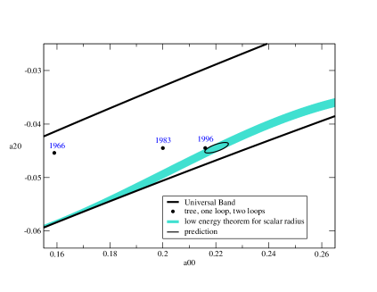
Figure 15: Constraints imposed on the $S$-wave scattering lengths by chiral symmetry. The three circles illustrate the prediction of the chiral perturbation theory at increasing order. The error ellipse represents the final result from Ref. [32], while the narrow, curved band indicates the region allowed in GChPT

E865 has performed this analysis, with the result [22]

$$a_{0}^{0}=0.216\pm 0.013\,({\mbox{stat}})\pm 0.002\,({\mbox{syst}})\pm 0.002\,({\mbox{theor}})\;.$$

The central value leads to $\bar{l}_{3}\simeq 6$, with an uncertainty of about 10 units. In the expansion (5.10), the second term amounts to a correction of about four percent at $\bar{l}_{3}$ =6. From this, one concludes that the first term in the mass expansion dominates by far: the motivation for a generalized scheme [30], with a small quark condensate and a large second term in (5.10) has evaporated, at least for $SU(2)\times SU(2)$.

7.4 Note added after the lectures

On the precision of the theoretical predictions for $\pi\pi$ scattering

In two recent papers [41], Peláez and Ynduráin evaluate some of the low energy observables of $\pi\pi$ scattering and obtain flat disagreement with our results [32] that I have described above. The authors work with unsubtracted dispersion relations, so that their results are very sensitive to the poorly known high energy behaviour of the scattering amplitude. They claim that the asymptotic representation we used in [36, 32] is incorrect and propose an alternative one. We have repeated [43] their calculations on the basis of the standard, subtracted fixed-$t$ dispersion relations, using their asymptotics. The outcome fully confirms our earlier findings. Moreover, we show that the Regge parametrization proposed by these authors for the region above 1.4 GeV violates crossing symmetry: Their ansatz is not consistent with the behaviour observed at low energies.

8 Outlook

Instead of a summary, I have provided at the school an outlook on topics not covered in the lectures. This outlook was based on the structure of the effective chiral lagrangian of the Standard Model [44] displayed in Table 1. The numbers in brackets denote the number of independent LECs . The numbers refer to $N_{f}=3$, except for the pieces with superscript $\pi N$.

Table 1: The effective lagrangian of the Standard Model [44]

${\cal L}_{\rm chiral\;order}$  ($\#$ of LECs)
${\cal L}_{p^{2}}(2)$+${\cal L}_{p^{4}}^{\rm odd}(0)$+ ${\cal L}_{G_{F}p^{2}}^{\Delta S=1}(2)$ +${\cal L}_{e^{2}p^{0}}^{\rm em}(1)$ +${\cal L}_{G_{8}e^{2}p^{0}}^{\rm emweak}(1)$
+ ${\cal L}_{p}^{\pi N}(1)$+${\cal L}_{p^{2}}^{\pi N}(7)$ +${\cal L}_{G_{8}p^{0}}^{MB,\Delta S=1}(2)$+ ${\cal L}_{G_{8}p}^{MB,\Delta S=1}(8)$ + ${\cal L}_{e^{2}p^{0}}^{\pi N,{\rm em}}(3)$
+ $\underline{{\cal L}_{p^{4}}^{\rm even}(10)}$+ $\underline{{\cal L}_{p^{6}}^{\rm odd}(32)}$ +$\underline{{\cal L}_{G_{8}p^{4}}^{\Delta S=1}(22)}$ +$\underline{{\cal L}_{e^{2}p^{2}}^{\rm em}(14)}$ + $\underline{{\cal L}_{G_{8}e^{2}p^{2}}^{\rm emweak}(14)}$
+ $\underline{{\cal L}_{e^{2}p}^{\rm leptons}(5)}$
+ $\underline{{\cal L}_{p^{3}}^{\pi N}(23)}$+ $\underline{{\cal L}_{p^{4}}^{\pi N}(118)}$ + $\underline{{\cal L}_{G_{8}p^{2}}^{MB,\Delta S=1}(?)}$ +$\underline{{\cal L}_{e^{2}p}^{\pi N,{\rm em}}(8)}$
+ $\underline{{\cal L}_{p^{6}}^{\rm even}(90)}$

The underlined lagrangians are fully renormalized: their divergence structure has been determined in a process independent manner. In the lectures, I had discussed aspects of ${\cal L}_{p^{2}},{\cal L}_{p^{4}}^{\rm even}$ and of ${\cal L}_{p^{6}}^{\rm even}$ in the $SU(2)\times SU(2)$ case. The above Table opens a very wide field of further applications.

Topics

Meson and baryon decays: electromagnetic, semileptonic, leptonic, non leptonic, rare and not so rare; decay constants $F_{\pi}$, $F_{K}$, $\ldots$; scattering amplitudes: $\pi\pi\rightarrow\pi\pi,\pi N\rightarrow\pi N,\gamma N\rightarrow\pi N,\ldots$; mixing angles; quark mass ratios; large $N_{C}$ investigations; anomalies; isospin violation; weak matrix elements; quark condensate; hadronic atoms; lattice: $m_{q}\rightarrow 0,V\rightarrow\infty$; quenched ChPT.

In order to study nuclear physics in the framework of ChPT, the above lagrangian must still be enlarged. A vast amount of massive calculations in this topic have been performed by V. Bernard, E. Epelbaum, W. Glöckle, N. Kaiser, Ulf-G. Meißner and others, see e.g. [46]. This method has allowed one to put theoretical nuclear physics on a sound basis.

For recent contributions to the topics just mentioned, see [47, 48].

Acknowledgements

It is a pleasure to thank the organizers of this Winter School for the warm hospitality, for the perfect organization of the School and for the very pleasant weather conditions. In addition, I thank Christoph Häfeli and Martin Schmid for providing me with many figures that I displayed during the lectures, and which are now incorporated partly also here. Finally, I thank Ulf-G. Meißner for carefully reading the manuscript. This work was supported in part by the Swiss National Science Foundation and by RTN, BBW-Contract No. 01.0357 and EC-Contract HPRN–CT2002–00311 (EURIDICE).

References

- [1] S. Weinberg, Phys. Rev. Lett. 17, 616 (1966).
- [2] S. Scherer, in: Advances in Nuclear Physics, Vol. 27, edited by J. W. Negele and E. W. Vogt (Kluwer Academic/Plenum Publishers, New York, 2002) [arXiv:hep-ph/0210398].
- [3] K. Hagiwara et al. [Particle Data Group Collaboration], Phys. Rev. D 66, 010001 (2002).
-
[4]
Y. Nambu,
Phys. Rev. Lett. 4, 380 (1960);
Phys. Rev. 117, 648 (1960);
Y. Nambu and G. Jona-Lasinio, Phys. Rev. 122, 345 (1961); ibid. 124, 246 (1961). -
[5]
J. Goldstone,
Nuovo Cim. 19, 154 (1961);
The paper by J. Goldstone, A. Salam and S. Weinberg, Phys. Rev. 127, 965 (1962), gives three different proofs of the theorem. - [6] H. Leutwyler, Phys. Lett. B 378, 313 (1996) [arXiv:hep-ph/9602366].
- [7] C. Vafa and E. Witten, Nucl. Phys. B 234, 173 (1984).
- [8] H. Araki and R. Haag, Comm. Math. Phys. 4, 77 (1967).
- [9] H. Lehmann, K. Symanzik and W. Zimmermann, Nuovo Cim. 1, 205 (1955).
- [10] W. E. Caswell and G. P. Lepage, Phys. Lett. B 167, 437 (1986).
- [11] A. Nyffeler and A. Schenk, Annals Phys. 241, 301 (1995) [arXiv:hep-ph/9409436].
- [12] J. Gasser and H. Leutwyler, Annals Phys. 158, 142 (1984).
- [13] S. Weinberg, Physica A 96, 327 (1979).
- [14] H. Leutwyler, Chiral Effective Lagrangians, in: Recent Aspects of Quantum Fields, Proceedings of the XXX. Internationale Universitätswochen für Kern- und Teilchenphysik, Schladming, Austria, Feb. 27 - March 8, 1991, Springer Lecture Notes in Physics, Vol. 396, H. Mitter, H. Gausterer (eds.).
- [15] A. V. Manohar, Effective Field Theories, in: Perturbative and Nonperturbative Aspects of Quantum Field Theory, Proceedings of the 35. Internationale Universitätswochen für Kern- und Teilchenphysik, Schladming, Austria, March 2-9, 1996, Springer Lecture Notes in Physics, Vol. 479, H. Latal, W. Schweiger (eds.), [arXiv:hep-ph/9606222].
- [16] G. Ecker, Chiral Symmetry, in: Broken Symmetries, Proceedings of the 37. Internationale Universitätswochen für Kern- und Teilchenphysik, Schladming, Austria, February 28 - March 7, 1998, Springer Lecture Notes in Physics, Vol. 521, L. Mathelitsch, W. Plessas (eds.), [arXiv:hep-ph/9805500].
- [17] H. Leutwyler, Annals Phys. 235, 165 (1994) [arXiv:hep-ph/9311274].
- [18] J. Bijnens, G. Colangelo and G. Ecker, JHEP 9902, 020 (1999) [arXiv:hep-ph/9902437]; Annals Phys. 280, 100 (2000) [arXiv:hep-ph/9907333].
-
[19]
T. Ebertshauser, H. W. Fearing and S. Scherer,
Phys. Rev. D 65, 054033 (2002)
[arXiv:hep-ph/0110261];
J. Bijnens, L. Girlanda and P. Talavera, Eur. Phys. J. C 23, 539 (2002) [arXiv:hep-ph/0110400]. -
[20]
J. Heitger, R. Sommer and H. Wittig [ALPHA Collaboration],
Nucl. Phys. B 588, 377 (2000)
[arXiv:hep-lat/0006026];
A. C. Irving, C. McNeile, C. Michael, K. J. Sharkey and H. Wittig [UKQCD Collaboration], Phys. Lett. B 518, 243 (2001) [arXiv:hep-lat/0107023];
D. R. Nelson, G. T. Fleming and G. W. Kilcup, Nucl. Phys. Proc. Suppl. 106, 221 (2002) [arXiv:hep-lat/0110112];
G. T. Fleming, D. R. Nelson and G. W. Kilcup, Nucl. Phys. Proc. Suppl. 119, 245 (2003) [arXiv:hep-lat/0209141];
F. Farchioni, C. Gebert, I. Montvay and L. Scorzato [qq+q Collaboration], arXiv:hep-lat/0209142;
F. Farchioni, C. Gebert, I. Montvay, E. Scholz and L. Scorzato [qq+q Collaboration], Phys. Lett. B 561, 102 (2003) [arXiv:hep-lat/0302011];
- [21] F. Farchioni, I. Montvay, E. Scholz and L. Scorzato [qq+q Collaboration], Eur. Phys. J. C 31, 227 (2003) [arXiv:hep-lat/0307002].
- [22] S. Pislak et al. [BNL-E865 Collaboration], Phys. Rev. Lett. 87, 221801 (2001) [arXiv:hep-ex/0106071]; Phys. Rev. D 67, 072004 (2003) [arXiv:hep-ex/0301040].
-
[23]
R. Batley et al. [NA48-Collaboration], Addendum III
(to Proposal P253/
CERN/SPSC) for a Precision Measurement of Charged Kaon Decay Parameters with an extended NA48 Setup, CERN/SPSC/P253 add. 3, Jan. 16, 2000. - [24] L. Maiani, G. Pancheri and N. Paver (eds.), The Second DANE Physics Handbook (INFN-LNF-Divisione Ricerca, SIS-Ufficio Publicazioni, Frascati, 1995).
- [25] B. Adeva et al., CERN proposal CERN/SPSLC 95-1, 1995.
- [26] H. Leutwyler, Electromagnetic form factor of the pion, in: Continuous Advances in QCD 2002: Arkadyfest – honoring the 60th birthday of Prof. Arkady Vainshtein, K. A. Olive, M. A. Shifman and M. B. Voloshin (eds.), World Scientific, 2003, [arXiv:hep-ph/0212324].
- [27] S. Deser, M. L. Goldberger, K. Baumann and W. Thirring, Phys. Rev. 96, 774 (1954).
-
[28]
J. Gasser, V. E. Lyubovitskij, A. Rusetsky and A. Gall,
Phys. Rev. D 64, 016008 (2001)
[arXiv:hep-ph/0103157];
J. Gasser, V. E. Lyubovitskij and A. Rusetsky, Phys. Lett. B 471, 244 (1999) [arXiv:hep-ph/9910438];
H. Sazdjian, Phys. Lett. B 490, 203 (2000) [arXiv:hep-ph/0004226]; arXiv:hep-ph/0012228.
Recent work on related matters is described in
A. Gashi, G. Rasche, G. C. Oades and W. S. Woolcock, Nucl. Phys. A 628, 101 (1998) [arXiv:nucl-th/9704017];
H. Jallouli and H. Sazdjian, Phys. Rev. D 58, 014011 (1998) [arXiv:hep-ph/9706450];
P. Labelle and K. Buckley [arXiv:hep-ph/9804201];
M.A. Ivanov, V.E. Lyubovitskij, E.Z. Lipartia and A.G. Rusetsky, Phys. Rev. D 58, 094024 (1998) [arXiv:hep-ph/9805356];
P. Minkowski, in: Proceedings of the International Workshop Hadronic Atoms and Positronium in the Standard Model, Dubna, 26-31 May 1998, M.A. Ivanov at al. (eds.), Dubna 1998 [arXiv:hep-ph/9808387];
E.A. Kuraev, Phys. Atom. Nucl. 61, 239 (1998);
U. Jentschura, G. Soff, V. Ivanov and S.G. Karshenboim, Phys. Lett. A 241, 351 (1998);
B.R. Holstein, Phys. Rev. D 60, 114030 (1999) [arXiv:nucl-th/9901041];
X. Kong and F. Ravndal, Phys. Rev. D 59, 014031 (1999); ibid. D 61, 077506 (2000) [arXiv:hep-ph/9905539];
H. W. Hammer and J. N. Ng, Eur. Phys. J. A 6, 115 (1999) [arXiv:hep-ph/9902284];
D. Eiras and J. Soto, Phys. Rev. D 61, 114027 (2000) [arXiv:hep-ph/9905543]; Phys. Lett. B 491, 101 (2000) [arXiv:hep-ph/0005066]. - [29] L. Rosselet et al., Phys. Rev. D 15, 574 (1977).
- [30] M. Knecht, B. Moussallam, J. Stern and N. H. Fuchs, Nucl. Phys. B 457, 513 (1995) [arXiv:hep-ph/9507319]; ibid. B 471, 445 (1996) [arXiv:hep-ph/9512404].
- [31] J. Bijnens, G. Colangelo, G. Ecker, J. Gasser and M. E. Sainio, Phys. Lett. B 374, 210 (1996) [arXiv:hep-ph/9511397]; Nucl. Phys. B 508, 263 (1997) [Erratum-ibid. B 517, 639 (1998)] [arXiv:hep-ph/9707291].
- [32] G. Colangelo, J. Gasser and H. Leutwyler, Nucl. Phys. B 603, 125 (2001) [arXiv:hep-ph/0103088].
- [33] S. M. Roy, Phys. Lett. B 36, 353 (1971).
-
[34]
J. L. Basdevant, J. C. Le Guillou and H. Navelet,
Nuovo Cim. A 7, 363 (1972);
M.R. Pennington and S.D. Protopopescu, Phys. Rev. D 7, 1429 (1973); ibid. D 7, 2591 (1973);
J. L. Basdevant, C. D. Froggatt and J. L. Petersen, Phys. Lett. B 41, 173 (1972); ibid. 178; ibid. B 72, 413 (1974);
J. L. Petersen, Acta Phys. Austriaca Suppl. 13, 291 (1974); Yellow report CERN 77-04 (1977);
C. D. Froggatt and J. L. Petersen, Nucl. Phys. B 91, 454 (1975); ibid. B 104, 186 (1976) (E); ibid. B 129, 89 (1977);
D. Morgan and M.R. Pennington, in ref. [24], p. 193;
P. Büttiker, Comparison of Chiral Perturbation Theory with a Dispersive Analysis of Scattering, PhD thesis, Universität Bern, 1996;
B. Ananthanarayan and P. Büttiker, Phys. Rev. D 54, 1125 (1996) [arXiv:hep-ph/9601285]; Phys. Rev. D 54, 5501 (1996) [arXiv:hep-ph/9604217]; Phys. Lett. B 415, 402 (1997) [arXiv:hep-ph/9707305] and in ref. [35], p. 370;
O. O. Patarakin, V. N. Tikhonov and K. N. Mukhin, Nucl. Phys. A 598, 335 (1996);
O. O. Patarakin (for the CHAOS collaboration), in ref. [35], p. 376, and arXiv:hep-ph/9711361;
M. Kermani et al. [CHAOS Collaboration], Phys. Rev. C 58, 3431 (1998);
B. Loiseau, R. Kaminski and L. Lesniak, Newslett. 16, 349 (2002) [arXiv:hep-ph/0110055];
R. Kaminski, L. Lesniak and B. Loiseau, arXiv:hep-ph/0207063; Phys. Lett. B 551, 241 (2003) [arXiv:hep-ph/0210334]. - [35] A.M. Bernstein, D. Drechsel and T. Walcher (eds.), Chiral Dynamics: Theory and Experiment, Workshop held in Mainz, Germany, 1-5 Sept. 1997, Lecture Notes in Physics Vol. 513, Springer, 1997.
- [36] B. Ananthanarayan, G. Colangelo, J. Gasser and H. Leutwyler, Phys. Rept. 353, 207 (2001) [arXiv:hep-ph/0005297].
- [37] G.Wanders, Helv. Phys. Acta 39, 228 (1966).
- [38] G. Colangelo, J. Gasser and H. Leutwyler, Phys. Lett. B 488, 261 (2000) [arXiv:hep-ph/0007112].
- [39] G. Colangelo, J. Gasser and H. Leutwyler, Phys. Rev. Lett. 86, 5008 (2001) [arXiv:hep-ph/0103063].
- [40] I thank H. Leutwyler for providing me with this figure.
- [41] J. R. Peláez and F. J. Ynduráin, Phys. Rev. D 68, 074005 (2003) [arXiv:hep-ph/0304067]; F. J. Ynduráin, arXiv:hep-ph/0310206; see also [42].
-
[42]