Subleading shape function contributions to the hadronic invariant mass spectrum in $\bar{B}\to X_{u}\ell\bar{\nu}_{\ell}$ decay

Abstract

We study the $O(\Lambda_{\rm QCD}/m_{b})$ corrections to the singly and doubly differential hadronic invariant mass spectra $d\Gamma/ds_{H}$ and $d\Gamma/ds_{H}dq^{2}$ in $\bar{B}\to X_{u}\ell\bar{\nu}_{\ell}$ decays, and discuss the implications for the extraction of the CKM matrix element $|V_{ub}|$. Using simple models for the subleading shape functions, the effects of subleading operators are estimated to be at the few percent level for experimentally relevant cuts. The subleading corrections proportional to the leading shape function are larger, but largely cancel in the relation between the hadronic invariant mass spectrum and the photon spectrum in $\bar{B}\to X_{s}\gamma$. We also discuss the applicability of the usual prescription of convoluting the partonic level rate with the leading light-cone wavefunction of the $b$ quark to subleading order.

I Introduction

The CKM parameter $|V_{ub}|$ is of phenomenological interest both because it is a basic parameter of the Standard Model and because of the role it plays in precision studies of $CP$ violation in the $B$ meson system. Currently, the theoretically cleanest determinations of $|V_{ub}|$ come from inclusive semileptonic decays, which are not sensitive to the details of hadronization.

For sufficiently inclusive observables, inclusive decay rates may be written as an expansion in local operators operefs . The leading order result corresponds to the decay of a free $b$ quark to quarks and gluons, while the subleading corrections, proportional to powers of $\Lambda_{\rm QCD}/m_{b}$, describe the deviations from the parton model. Up to $O(\Lambda_{\rm QCD}^{2}/m_{b}^{2})$, only two operators arise,

$$\lambda_{1}\equiv{1\over 2m_{B}}\langle\bar{B}|\bar{h}_{v}(iD)^{2}h_{v}|\bar{B}\rangle,\ \lambda_{2}(\mu)\equiv{1\over 6m_{B}}\langle\bar{B}|\bar{h}_{v}\sigma^{\mu\nu}G_{\mu\nu}h_{v}|\bar{B}\rangle.$$ (1)

The $B-B^{*}$ mass splitting determines $\lambda_{2}(m_{b})\simeq 0.12\,\mbox{GeV}^{2}$, while a recent fit to moments of the charged lepton spectrum in semileptonic $b\to c$ decay obtained cleolepton

$$m_{b}^{1S}=4.82\pm 0.07_{E}\pm 0.11_{T}\,\mbox{GeV},\ \ \lambda_{1}=-0.25\pm 0.02_{ST}\pm 0.05_{SY}\pm 0.14_{T}\,\mbox{GeV}^{2}$$ (2)

where $m_{b}^{1S}$ is the short-distance “1S mass” of the $b$ quark upsexpansion1 ; upsexpansion2 . (Moments of other spectra give similar results moments1 ; moments2 .) These uncertainties correspond to an uncertainty of $\sim 5\%$ in the relation between $|V_{ub}|$ and the inclusive $\bar{B}\to X_{u}\ell\bar{\nu}_{\ell}$ width upsexpansion1 ; burels .

Unfortunately, the semileptonic $b\to u$ decay rate is difficult to measure experimentally, because of the large background from charmed final states. As a result, there has been much theoretical and experimental interest in the decay rate in restricted regions of phase space where the charm background is absent. Of particular interest have been the large lepton energy region, $E_{\ell}>(m_{B}^{2}-m_{D}^{2})/2m_{B}$, the low hadronic invariant mass region, $m_{X}\equiv\sqrt{s_{H}}<m_{D}$ lowmX , the large lepton invariant mass region $q^{2}>(m_{B}-m_{D})^{2}$ BLLqsq , and combinations of these BLLmixed . The charged lepton cut is the easiest to implement experimentally, while the hadronic mass cut has the advantage that it contains roughly $80\%$ of the semileptonic rate dFN . However, in both cases the kinematic cuts constrain the final hadronic state to consist of energetic, low-invariant mass hadrons, and the local OPE breaks down (this is not the case for the large $q^{2}$ region or for appropriately chosen mixed cuts). In this case, the relevant spectrum is determined at leading order in $\Lambda_{\rm QCD}/m_{b}$ by the light-cone distribution function of the $b$ quark in the meson shapeleading1 ; shapeleading2 ,

$$f(\omega)\equiv\frac{\langle\bar{B}|\bar{b}\;\delta(\omega+in\cdot\hat{D})\;b|\bar{B}\rangle}{2m_{B}}$$ (3)

where $n^{\mu}$ is a light-like vector, and hatted variables are normalized to $m_{b}$: $\hat{D}^{\mu}\equiv D^{\mu}/m_{b}$. $f(\omega)$ is often referred to as the shape function, and corresponds to resumming an infinite series of local operators in the usual OPE. The physical spectra are determined by convoluting the shape function with the appropriate kinematic functions:

$${1\over\Gamma_{0}}{d\Gamma\over d\hat{E}_{\ell}}(\bar{B}\to X_{u}\ell\bar{\nu}_{\ell}) = 4\int\theta(1-2\hat{E}_{\ell}-\omega)f(\omega)\;d\omega+\dots$$ (4)

$${1\over\Gamma_{0}}{d\Gamma\over d\hat{s}_{H}}(\bar{B}\to X_{u}\ell\bar{\nu}_{\ell}) = \int{2\hat{s}_{H}^{2}(3\omega-2\hat{s}_{H})\over\omega^{4}}\theta(\omega-\hat{s}_{H})f(\omega-\hat{\Delta})\;d\omega+\dots$$ (5)

where $1-2\hat{E}_{\ell}\lesssim\Lambda_{\rm QCD}/m_{b}$, $\hat{s}_{H}\lesssim\Lambda_{\rm QCD}/m_{b}$ and $\Delta\equiv m_{B}-m_{b}$.

Since $f(\omega)$ also determines the shape of the photon spectrum in $\bar{B}\to X_{s}\gamma$ at leading order,

$${1\over\Gamma_{0}^{s}}{d\Gamma\over d\hat{E}_{\gamma}}(\bar{B}\to X_{s}\gamma)=2f(1-2\hat{E}_{\gamma})+\dots$$ (6)

there has been much interest in extracting $f(\omega)$ from radiative $B$ decay and applying it to semileptonic decay. However, the relations (4–6) hold only at tree level and at leading order in $\Lambda_{\rm QCD}/m_{b}$, so a precision determination of $|V_{ub}|$ requires an understanding of the size of the corrections. Radiative corrections were considered in shapeleading1 ; shapeleading2 ; shaperadiative ; Bauer:2003pi , while $O(\Lambda_{\rm QCD}/m_{b})$ corrections have been studied more recently in blm01 ; blm02 ; mn02 ; llw02 . In blm01 , the nonlocal distribution functions arising at subleading order were enumerated, and their contribution to $\bar{B}\to X_{s}\gamma$ decay was studied. In blm02 , the corresponding corrections to the lepton endpoint spectrum in $\bar{B}\to X_{u}\ell\bar{\nu}_{\ell}$ decay were studied, and it was shown that these effects were potentially large. Similar results were obtained in llw02 , where the sub-subleading contribution from annihilation graphs was also shown to be large. In this paper, we study the subleading corrections to the hadronic invariant mass spectrum in semileptonic $b\to u$ decay, and estimate the theoretical uncertainties introduced by these terms. In addition, we present results for the doubly differential spectrum $d\Gamma/ds_{H}dq^{2}$ at leading and subleading order.

II Matching Calculation

II.1 The full theory spectrum

In the shape function region the final hadronic state has large energy but small invariant mass, and so its momentum lies close to the light-cone. It is therefore convenient to introduce two light-like vectors $n^{\mu}$ and $\bar{n}^{\mu}$ related to the velocity of the heavy meson $v^{\mu}$ by $v^{\mu}={\textstyle{1\over 2}}(n^{\mu}+\bar{n}^{\mu})$, and satisfying

$$n^{2}=\bar{n}^{2}=0,\quad v\cdot n=v\cdot\bar{n}=1,\quad n\cdot\bar{n}=2.$$ (7)

In the frame in which the $B$ meson is at rest, these vectors are given by $n^{\mu}=(1,0,0,1)$, $\bar{n}^{\mu}=(1,0,0,-1)$ and $v^{\mu}=(1,0,0,0)$. The projection of an arbitrary four-vector $a^{\alpha}$ onto the directions which are perpendicular to the light-cone is given by $a_{\perp}^{\alpha}=g^{\alpha\beta}_{\perp}a_{\beta}$, where

$$g^{\mu\nu}_{\perp}=g^{\mu\nu}-\frac{1}{2}\left(n^{\mu}\bar{n}^{\nu}+\bar{n}^{\mu}n^{\nu}\right)\,.$$ (8)

Choosing our axes such that the momentum transfer to the leptons $\vec{q}$ is in the $-\vec{n}$ direction, we can write $q^{\mu}={\textstyle{1\over 2}}n\cdot q\;\bar{n}^{\mu}+{\textstyle{1\over 2}}\bar{n}\cdot q\;n^{\mu}$, the decay rate takes a particularly simple form in terms of the variables $n\cdot q$ and $\bar{n}\cdot q$:

$$d\Gamma(\bar{B}\to X_{u}\ell\bar{\nu}_{\ell})=96\pi\;\Gamma_{0}\;W_{\mu\nu}L^{\mu\nu}(n\cdot\hat{q}-\bar{n}\cdot\hat{q})^{2}\theta(\bar{n}\cdot\hat{q})\theta(n\cdot\hat{q}-\bar{n}\cdot\hat{q})dn\cdot\hat{q}\;d\bar{n}\cdot\hat{q}$$ (9)

where

$$\Gamma_{0}=\frac{G_{F}^{2}|V_{ub}|^{2}m_{b}^{5}}{192\pi^{3}}.$$ (10)

The hadron tensor $W^{\mu\nu}$ is defined by

$$W^{\mu\nu}\equiv-\frac{1}{\pi}\mbox{Im}\left(-i\int d^{4}x\,e^{-iq\cdot x}\frac{\langle\bar{B}|T[J_{L}^{\dagger\mu}(x)J_{L}^{\nu}(0)]|\bar{B}\rangle}{2m_{B}}\right),$$ (11)

where the weak current is $J_{L}^{\mu}=\bar{u}\gamma^{\mu}(1-\gamma_{5})b$, while the lepton tensor is

$$L^{\mu\nu}\equiv\int\;d\Pi_{2}(q;p_{\ell},p_{\nu})\mbox{Tr}[{\hbox to0.0pt{$p$\hss}/}_{\nu}\gamma^{\mu}{\hbox to0.0pt{$p$\hss}/}_{\ell}\gamma^{\nu}P_{L}]=\frac{1}{12\pi}(q^{\mu}q^{\nu}-q^{2}g^{\mu\nu})$$ (12)

and $P_{L}\equiv{\textstyle{1\over 2}}(1-\gamma_{5})$.

To calculate the hadronic invariant mass spectrum we switch to the variables $(s_{H},q^{2})$. These are related to the variables in Eq. (9) by

$$s_{H} = (m_{B}-n\cdot q)(m_{B}-n\cdot\bar{q})$$ (13)

$$= (m_{b}+\Delta-n\cdot q)(m_{b}+\Delta-\bar{n}\cdot q)$$

$$q^{2} = n\cdot q\;\bar{n}\cdot q$$ (14)

and

$$\frac{d\Gamma}{dn\cdot q\,d\bar{n}\cdot q}=\sqrt{((m_{b}+\Delta)^{2}+q^{2}-s_{H})^{2}-4(m_{b}+\Delta)^{2}q^{2}}\frac{d\Gamma}{ds_{H}\,dq^{2}}.$$ (15)

Here $\Delta=m_{B}-m_{b}$ is the difference between the $B$ meson mass and the $b$ quark mass. It is ${\cal O}(\Lambda_{\rm QCD})$ and has an expansion in terms of HQET parameters

$$\Delta=\bar{\Lambda}-\frac{\lambda_{1}+3\lambda_{2}}{2m_{b}}+\cdots\ .$$ (16)

Since $\Delta$ simply enters in the definition of $s_{H}$, it is unrelated to the $1/m$ expansion in the OPE, so we will not expand it via Eq. (16). With this change of variables, we define the correlator $T(s_{H},q^{2})$ by

$$\frac{1}{\Gamma_{0}}\frac{d\Gamma}{ds_{H}\;dq^{2}}={1\over 2m_{B}}\langle\bar{B}|T(s_{H},q^{2})|\bar{B}\rangle.$$ (17)

In Ref. blm01 a nonlocal expansion was performed for the hadron tensor $W^{\mu\nu}$, based on the power counting

$$(m_{b}v-q)\cdot\bar{n} = m_{b}-q\cdot\bar{n}\sim{\cal O}(m_{b}),$$

$$(m_{b}v-q)\cdot n = m_{b}-q\cdot n\sim{\cal O}(\Lambda_{\rm QCD}),$$ (18)

$$k^{\mu} \sim {\cal O}(\Lambda_{\rm QCD}).$$

where the heavy quark momentum is defined as $p_{b}^{\mu}=m_{b}v^{\mu}+k^{\mu}$. However, the limits of phase space integration in Eq. (9) include regions of phase space where this power counting is violated. Hence, to keep our power counting consistent, we do not perform a nonlocal OPE for $W^{\mu\nu}$, but rather for $T(s_{H},q^{2})$. In these variables, the shape function region corresponds to the region of low invariant mass,

$$s_{H}\sim{\cal O}(\Lambda_{\rm QCD}m_{b}).$$ (19)

Since $\Delta\sim\Lambda_{\rm QCD}$ and $k^{\mu}\sim\Lambda_{\rm QCD}$, expanding the light quark propagator in powers of $\Lambda_{\rm QCD}/m_{b}$ gives at leading order

$$\frac{i{\hbox to0.0pt{$p$\hss}/}_{u}}{p_{u}^{2}}=\frac{i{\hbox to0.0pt{$n$\hss}/}}{2m_{b}}\frac{(1-\hat{q}^{2})}{[\hat{s}_{H}-(\hat{\Delta}-n\cdot\hat{k})(1-\hat{q}^{2})]}+\cdots\$$ (20)

(where $\hat{\Delta}\equiv\bar{\Lambda}/m_{b}$). Since both terms in the denominator are $O(\Lambda_{\rm QCD}/m_{b})$, $T(s_{H},q^{2})$ cannot be expanded in powers of $k^{\mu}$ and matched onto local operators (unless we also are restricted to large $q^{2}$, such that $1-\hat{q}^{2}\ll 1$, in which case the second term in the denominator is subleading, and a local OPE may be performed BLLqsq ; BLLmixed ). Instead, the OPE takes the schematic form

$$T(\hat{s}_{H},\hat{q}^{2})=\sum_{n}\int C_{n}(\omega,\hat{s}_{H},\hat{q}^{2}){\cal O}_{n}(\omega)d\omega$$ (21)

where the ${\cal O}_{n}(\omega)$’s are bilocal operators in which the two points are separated along the light cone.

II.2 Nonlocal operators

In Refs. blm01 ; blm02 , it was shown that up to subleading order in $\Lambda_{\rm QCD}/m_{b}$, the following operators were required in the OPE (21):

$$O_{0}(\omega) = \bar{h}_{v}\delta(\omega+in\cdot\hat{D})h_{v}$$ (22)

$$O_{1}^{\mu}(\omega) = \bar{h}_{v}\{i\hat{D}^{\mu},\delta(\omega+in\cdot\hat{D})\}h_{v}$$

$$O_{2}^{\mu}(\omega) = \bar{h}_{v}[i\hat{D}^{\mu},\delta(\omega+in\cdot\hat{D})]h_{v}$$

$$O_{3}(\omega) = \int\!d\omega_{1}d\omega_{2}\,\delta(\omega_{1},\omega_{2};\omega)\bar{h}_{v}\delta(in\cdot\hat{D}\!+\!\omega_{2})g^{\mu\nu}_{\perp}\{i\hat{D}_{\mu},i\hat{D}_{\nu}\}\delta(in\cdot\hat{D}\!+\!\omega_{1})h_{v},$$

$$O_{4}(\omega) = -\int\!d\omega_{1}d\omega_{2}\,\delta(\omega_{1},\omega_{2};\omega)\bar{h}_{v}\delta(in\cdot\hat{D}\!+\!\omega_{2})\epsilon_{\perp}^{\mu\nu}[i\hat{D}_{\mu},i\hat{D}_{\nu}]\delta(in\cdot\hat{D}\!+\!\omega_{1})h_{v}\,,$$

$$P_{0}^{\eta}(\omega) = \bar{h}_{v}\delta(\omega+in\cdot\hat{D})\gamma^{\eta}\gamma_{5}h_{v}$$

$$P_{1}^{\mu\eta}(\omega) = \bar{h}_{v}\{i\hat{D}^{\mu},\delta(\omega+in\cdot\hat{D})\}\gamma^{\eta}\gamma_{5}h_{v}$$

$$P_{2}^{\mu\eta}(\omega) = \bar{h}_{v}[i\hat{D}^{\mu},\delta(\omega+in\cdot\hat{D})]\gamma^{\eta}\gamma_{5}h_{v}$$

$$P_{3}^{\eta}(\omega) = \int\!d\omega_{1}d\omega_{2}\,\delta(\omega_{1},\omega_{2};\omega)\bar{h}_{v}\delta(in\cdot\hat{D}\!+\!\omega_{2})g^{\mu\nu}_{\perp}\{i\hat{D}_{\mu},i\hat{D}_{\nu}\}\delta(in\cdot\hat{D}\!+\!\omega_{1})\gamma^{\eta}\gamma_{5}h_{v},$$

$$P_{4}^{\eta}(\omega) = -\int\!d\omega_{1}d\omega_{2}\,\delta(\omega_{1},\omega_{2};\omega)\bar{h}_{v}\delta(in\cdot\hat{D}\!+\!\omega_{2})\epsilon_{\perp}^{\mu\nu}[i\hat{D}_{\mu},i\hat{D}_{\nu}]\delta(in\cdot\hat{D}\!+\!\omega_{1})\gamma^{\eta}\gamma_{5}h_{v}\,,$$

where the $h_{v}$’s are heavy quark fields in HQET, and we have defined

$$\delta(\omega_{1},\omega_{2};\omega)=\frac{\delta(\omega-\omega_{1})-\delta(\omega-\omega_{2})}{\omega_{1}-\omega_{2}}$$ (23)

and

$$\epsilon_{\perp}^{\alpha\beta}=\epsilon^{\alpha\beta\sigma\rho}v_{\sigma}n_{\rho}.$$ (24)

These definitions differ slightly from the definitions in Refs. blm01 ; blm02 , because we have chosen to normalize all momenta to $m_{b}$, to keep the resulting formulas simpler.

It is convenient to calculate the matching conditions onto a slightly different set of operators, defined in terms of full QCD $b$ quark fields:

$$Q_{0}(\omega,\Gamma) = \bar{b}\delta(in\cdot\hat{{\cal D}}+\omega)\Gamma b\,$$ (25)

$$\ Q_{1}^{\mu}(\omega,\Gamma) = \bar{b}\left\{i\hat{{\cal D}}^{\mu},\delta(in\cdot\hat{{\cal D}}+\omega)\right\}\Gamma b,$$

$$Q_{2}^{\mu}(\omega,\Gamma) = \bar{b}\left[i\hat{{\cal D}}^{\mu},\delta(in\cdot\hat{{\cal D}}+\omega)\right]\Gamma b,$$

$$Q_{3}(\omega,\Gamma) = \!\!\int\!d\omega_{1}d\omega_{2}\,\delta(\omega_{1},\omega_{2};\omega)\bar{b}\delta(in\cdot\hat{{\cal D}}\!+\!\omega_{2})g^{\mu\nu}_{\perp}\{i\hat{{\cal D}}_{\mu},i\hat{{\cal D}}_{\nu}\}\delta(in\cdot\hat{{\cal D}}\!+\!\omega_{1})\Gamma b,$$

$$Q_{4}(\omega,\Gamma) = -\!\!\int\!d\omega_{1}d\omega_{2}\,\delta(\omega_{1},\omega_{2};\omega)\bar{b}\delta(in\cdot\hat{{\cal D}}\!+\!\omega_{2})\epsilon_{\perp}^{\mu\nu}[i\hat{{\cal D}}_{\mu},i\hat{{\cal D}}_{\nu}]\delta(in\cdot\hat{{\cal D}}\!+\!\omega_{1})\Gamma b\,.$$

We have defined

$$i{\cal D}^{\mu}\equiv iD^{\mu}-m_{b}v^{\mu}$$ (26)

so that $i{\cal D}^{\mu}$ acting on the $b$ fields just bring down factors of the residual momentum $k^{\mu}$. The Feynman rules for the $O_{i}$’s and $P_{i}$’s are given in blm01 ; blm02 . The rules for the $Q_{i}$’s are given in $n\cdot A=0$ gauge in Fig. 1, where we have defined

$$\delta_{\pm}(x)=\delta(\omega+n\cdot\hat{k}+x)\pm\delta(\omega+n\cdot\hat{k}).$$ (27)

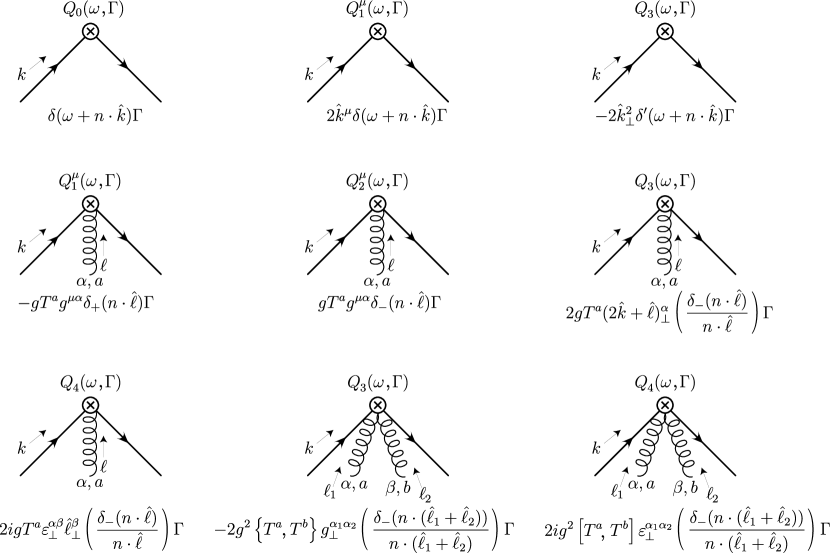
Figure 1: Feynman rules for the operators $Q_{i}(\omega,\Gamma)$ in $n\cdot A=0$ gauge. We have defined $\delta_{\pm}(x)=\delta(\omega+n\cdot\hat{k}+x)\pm\delta(\omega+n\cdot\hat{k})$.

It is simpler to match onto the $Q_{i}$’s initially since this matching does not require us to relate the QCD quark fields to HQET quark fields. However, because the additional symmetries of HQET reduce the number of independent functions needed to parametrize the matrix elements, it is convenient to then express the $Q_{i}$’s in terms of the $O_{i}$’s and $P_{i}$’s. For an arbitrary Dirac structure $\Gamma$ we have

$$\bar{b}\delta(\omega+in\cdot\hat{{\cal D}})\Gamma b = \bar{h}_{v}\left(1+\frac{iD\hskip-6.49994pt/}{2m_{b}}\right)\delta(\omega+in\cdot\hat{D})\Gamma\left(1+\frac{iD\hskip-6.49994pt/}{2m_{b}}\right)h_{v}+\cdots$$

$$= \frac{1}{2}\mbox{Tr}[\Gamma P_{+}]O_{0}(\omega)-\frac{1}{2}\mbox{Tr}[\Gamma s_{\eta}]P_{0}^{\eta}(\omega)$$

$$+ \frac{1}{8}\left(\mbox{Tr}[\gamma_{\lambda}\Gamma P_{+}]+\mbox{Tr}[\Gamma\gamma_{\lambda}P_{+}]\right)O_{1}^{\lambda}(\omega)$$

$$+ \frac{1}{8}\left(\mbox{Tr}[\gamma_{\lambda}\Gamma P_{+}]-\mbox{Tr}[\Gamma\gamma_{\lambda}P_{+}]\right)O_{2}^{\lambda}(\omega)$$

$$- \frac{1}{8}\left(\mbox{Tr}[\gamma_{\lambda}\Gamma s_{\eta}]+\mbox{Tr}[\Gamma\gamma_{\lambda}s_{\eta}]\right)P_{1}^{\lambda\eta}(\omega)$$

$$- \frac{1}{8}\left(\mbox{Tr}[\gamma_{\lambda}\Gamma s_{\eta}]-\mbox{Tr}[\Gamma\gamma_{\lambda}s_{\eta}]\right)P_{2}^{\lambda\eta}(\omega)+\cdots$$

where

$$P_{+}={\textstyle{1\over 2}}(1+{\hbox to0.0pt{$v$\hss}/})\hskip 28.45274pt\mbox{and}\hskip 28.45274pts^{\eta}=P_{+}\gamma^{\eta}\gamma_{5}P_{+}$$ (29)

and we have used the fact that

$$\bar{h}_{v}\Gamma h_{v}=\frac{1}{2}\mbox{Tr}[\Gamma P_{+}]\bar{h}_{v}h_{v}-\frac{1}{2}\mbox{Tr}[\Gamma s_{\eta}]\bar{h}_{v}\gamma^{\eta}\gamma_{5}h_{v}.$$ (30)

For our purposes, we will only need the case $\Gamma=\gamma_{\sigma}P_{L}$, which allows us to write

$$Q_{0}(\omega,\gamma_{\sigma}P_{L}) = \frac{1}{2}v_{\sigma}O_{0}(\omega)-\frac{1}{2}(g_{\sigma\eta}-v_{\sigma}v_{\eta})P_{0}^{\eta}(\omega)$$

$$+ \frac{1}{4}g_{\lambda\sigma}O_{1}^{\lambda}(\omega)-\frac{1}{4}(g_{\sigma\eta}v_{\lambda}-g_{\lambda\eta}v_{\sigma})P_{1}^{\lambda\eta}(\omega)$$

$$+ \frac{1}{4}i\epsilon_{\sigma\lambda\eta\rho}v^{\rho}P_{2}^{\lambda\eta}(\omega)+\cdots$$

where the first line gives the leading order relation and subsequent lines contain the subleading correction.

Similar relations may be derived for the subleading operators, though in these cases it is not necessary to consider the subleading terms in the relation between the QCD operator and the HQET operator, such terms being of higher order overall. Thus we have

$$Q_{1}^{\mu}(\omega,\gamma_{\sigma}P_{L}) = {\textstyle{1\over 2}}v_{\sigma}O_{1}^{\mu}(\omega)-{\textstyle{1\over 2}}(g_{\eta\sigma}-v_{\eta}v_{\sigma})P_{1}^{\mu\eta}(\omega)+\cdots$$

$$Q_{2}^{\mu}(\omega,\gamma_{\sigma}P_{L}) = {\textstyle{1\over 2}}v_{\sigma}O_{2}^{\mu}(\omega)-{\textstyle{1\over 2}}(g_{\eta\sigma}-v_{\eta}v_{\sigma})P_{2}^{\mu\eta}(\omega)+\cdots$$ (32)

$$Q_{3}(\omega,\gamma_{\sigma}P_{L}) = {\textstyle{1\over 2}}v_{\sigma}O_{3}(\omega)-{\textstyle{1\over 2}}(g_{\eta\sigma}-v_{\eta}v_{\sigma})P_{3}^{\eta}(\omega)+\cdots$$

$$Q_{4}(\omega,\gamma_{\sigma}P_{L}) = {\textstyle{1\over 2}}v_{\sigma}O_{4}(\omega)-{\textstyle{1\over 2}}(g_{\eta\sigma}-v_{\eta}v_{\sigma})P_{4}^{\eta}(\omega)+\cdots\ .$$

The leading and subleading operators can then be completely parametrized in terms of five functions blm01 :

$$\langle\bar{B}|O_{0}(\omega)|\bar{B}\rangle = 2m_{B}\left(f(\omega)+\frac{t(\omega)}{2}\right)$$

$$\langle\bar{B}|O_{1}^{\mu}(\omega)|\bar{B}\rangle = 2m_{B}(n-\bar{n})^{\mu}\omega f(\omega)$$

$$\langle\bar{B}|O_{3}(\omega)|\bar{B}\rangle = 4m_{B}G_{2}(\omega)$$ (33)

$$\langle\bar{B}|P_{2}^{\mu\eta}(\omega)|\bar{B}\rangle = -2m_{B}i\epsilon_{\perp}^{\mu\eta}h_{1}(\omega)$$

$$\langle\bar{B}|P_{4}^{\eta}(\omega)|\bar{B}\rangle = 4m_{B}(v-n)^{\eta}H_{2}(\omega)$$

(once again, unlike in blm01 , these are defined here in terms of dimensionless arguments). The matrix elements of the other operators vanish.

II.3 Matching Conditions

The Wilson coefficients $C_{i}(\omega)$ of the operators in (21) are obtained by taking partonic matrix elements of both sides of the OPE. In particular we take zero-, one-, and two-gluon matrix elements, which corresponds to calculating the imaginary parts of the full-theory forward-scattering diagrams in Figure 2, multiplying by the lepton tensor $L^{\mu\nu}$ and appropriate phase space factors and matching them onto linear combinations of the effective diagrams. (The matching conditions may be completely determined from just the zero-gluon and one-gluon matrix elements, but we have calculated the rest as a check of the results.)

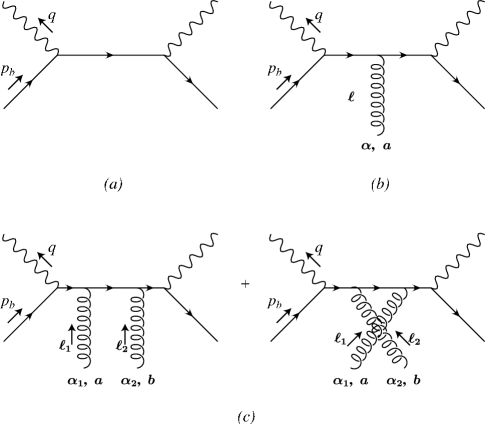
Figure 2: Full-theory forward scattering diagrams.

The lepton tensor has the expansion

$$L^{\mu\nu} = \frac{1}{12\pi}(q^{\mu}q^{\nu}-q^{2}g^{\mu\nu})$$

$$= \frac{m_{b}^{2}}{48\pi}\left\{\bar{n}^{\mu}\bar{n}^{\nu}+\hat{q}^{2}(n^{\mu}\bar{n}^{\nu}+\bar{n}^{\mu}n^{\nu})+\hat{q}^{4}n^{\mu}n^{\nu}-4\hat{q}^{2}\;g^{\mu\nu}\right\}$$

$$\hskip 8.5359pt-\frac{m_{b}^{2}}{24\pi}\frac{(\hat{s}_{H}-\hat{\Delta}(1-\hat{q}^{2}))}{(1-\hat{q}^{2})}\left\{\bar{n}^{\mu}\bar{n}^{\nu}-\hat{q}^{4}n^{\mu}n^{\nu}\right\}+\cdots.$$

(where we have used the decomposition $\hat{q}^{\mu}=n\cdot\hat{q}\bar{n}^{\mu}/2+\bar{n}\cdot\hat{q}n^{\mu}/2$), while the phase space factors give

$${(n\cdot\hat{q}-\bar{n}\cdot\hat{q})^{2}\over\sqrt{((1+\hat{\Delta})^{2}+\hat{q}^{2}-\hat{s}_{H})^{2}-4(1+\hat{\Delta})^{2}\hat{q}^{2}}}\theta(n\cdot\hat{q}-\bar{n}\cdot\hat{q})\theta(\bar{n}\cdot\hat{q})$$ (35)

$$\qquad=(1-\hat{q}^{2})\theta(\hat{q}^{2})\theta(1-\hat{q}^{2})$$

$$\qquad-{(1+\hat{q}^{2})\hat{s}_{H}-2\hat{q}^{2}(1-\hat{q}^{2})\hat{\Delta}\over 1-\hat{q}^{2}}\theta(\hat{q}^{2})\theta(1-\hat{q}^{2})-2\hat{s}_{H}\delta(1-\hat{q}^{2})+\dots$$

The zero-gluon diagram in Figure 2(a) gives the amplitude

$$iA_{0}=i\gamma^{\mu}\frac{{\hbox to0.0pt{$p$\hss}/}_{u}}{p_{u}^{2}}\gamma^{\nu}P_{L}.$$ (36)

Taking the imaginary part of this amplitude gives

$$-\frac{m_{b}}{\pi}\mbox{Im}[A_{0}] = \gamma^{\mu}{\hbox to0.0pt{$\hat{p}$\hss}/}_{u}\gamma^{\nu}P_{L}\delta(\hat{p}_{u}^{2})$$

$$= \frac{1}{2}\gamma^{\mu}{\hbox to0.0pt{$n$\hss}/}\gamma^{\nu}P_{L}\left[(1-\hat{q}^{2})\delta(h(n\cdot\hat{k}))\right.$$

$$\hskip 5.69046pt+\left.\left\{\frac{\hat{s}_{H}}{1-\hat{q}^{2}}(\hat{\Delta}(1-\hat{q}^{4})-\hat{s}_{H}\hat{q}^{2})-(1-\hat{q}^{2})\hat{k}_{\perp}^{2}\right\}\delta^{\prime}(h(n\cdot\hat{k}))\right]$$

$$\hskip 5.69046pt+\gamma^{\mu}{\hbox to0.0pt{$\hat{k}$\hss}/}_{\perp}\gamma^{\nu}P_{L}\delta(h(n\cdot\hat{k}))+\cdots$$

where we have expanded the amplitude to subleading order using (19) and we have simplified the expression by integrating by parts. The function $h(x)$ appearing in (II.3) is

$$h(x)=\hat{s}_{H}-(\hat{\Delta}-x)(1-\hat{q}^{2}).$$ (38)

Multiplying this result by the lepton tensor (II.3) and phase space factors (35), and expanding to subleading order we find

$$\langle b|T(\hat{s}_{H},\hat{q}^{2})|b\rangle=\sum_{n}\int d\omega\;\tilde{C}^{\sigma}_{n}(\omega,\hat{s}_{H},\hat{q}^{2})\langle b|Q_{n}(\omega,\gamma^{\sigma}P_{L})|b\rangle$$ (39)

where

$$\tilde{C}_{0}^{\sigma}(\omega,\hat{s}_{H},\hat{q}^{2}) = 4(1-\hat{q}^{2})^{2}(2\hat{q}^{2}n^{\sigma}+\bar{n}^{\sigma})\theta(\hat{q}^{2})\theta(1-\hat{q}^{2})\delta(h(-\omega))$$ (40)

$$\hskip 14.22636pt+8(1-\hat{q}^{2})((\hat{\Delta}(1-3\hat{q}^{2})-\omega\hat{q}^{2}(3-\hat{q}^{2}))n^{\sigma}$$

$$\hskip 28.45274pt-(\hat{\Delta}+\omega(2-\hat{q}^{2}))\bar{n}^{\sigma})\theta(\hat{q}^{2})\theta(1-\hat{q}^{2})\delta(h(-\omega))$$

$$\hskip 14.22636pt+4\hat{\Delta}\bar{n}^{\sigma}\delta(\hat{q}^{2})\delta(h(-\omega))+\cdots$$

$$\tilde{C}_{1}^{\mu\sigma}(\omega,\hat{s}_{H},\hat{q}^{2}) = 4\hat{q}^{2}(1-\hat{q}^{2})g_{\perp}^{\mu\sigma}\theta(\hat{q}^{2})\theta(1-\hat{q}^{2})\delta(h(-\omega))+\cdots$$

$$\tilde{C}_{3}^{\sigma}(\omega,\hat{s}_{H},\hat{q}^{2}) = -2(1-\hat{q}^{2})(2\hat{q}^{2}n^{\sigma}+\bar{n}^{\sigma})\theta(\hat{q}^{2})\theta(1-\hat{q}^{2})\delta(h(-\omega))+\cdots.$$

In order to determine the other matching coefficients, we calculate the one-gluon amplitude in Figure 2(b). Defining $\ell$ to be the incoming gluon momentum, we have

$$iA_{1}=igT^{a}\frac{\gamma^{\mu}({\hbox to0.0pt{$p$\hss}/}_{u}+{\hbox to0.0pt{$\ell$\hss}/})\gamma^{\alpha}{\hbox to0.0pt{$p$\hss}/}_{u}\gamma^{\nu}P_{L}}{(p_{u}+\ell)^{2}p_{u}^{2}}.$$ (41)

where $(\alpha,a)$ are, respectively, the Lorentz and colour indices of the gluon field.

Taking into account the two cuts which result from taking Im$[A_{1}]$ and scaling the gluon momentum as $\ell^{\alpha}\sim{\cal O}(\Lambda_{\rm QCD})$, we obtain, after expanding to leading order in $n\cdot A=0$ gauge,

$$-\frac{m_{b}^{2}}{\pi}\mbox{Im}[A_{1}] = -\frac{gT^{a}}{4}\gamma^{\mu}\left\{2\gamma^{\alpha}_{\perp}\tilde{\delta}_{+}(n\cdot\hat{\ell})+2{\hbox to0.0pt{$n$\hss}/}(2\hat{k}+\hat{\ell})_{\perp}^{\alpha}\left(\frac{\tilde{\delta}_{-}(n\cdot\hat{\ell})}{n\cdot\hat{\ell}}\right)\right.$$

$$+ \left.2i\epsilon_{\perp}^{\alpha\beta}\gamma_{\beta}\gamma_{5}\tilde{\delta}_{-}(n\cdot\hat{\ell})+2i\epsilon_{\perp}^{\alpha\beta}\hat{\ell}_{\perp\beta}{\hbox to0.0pt{$n$\hss}/}\gamma_{5}\left(\frac{\tilde{\delta}_{-}(n\cdot\hat{\ell})}{n\cdot\hat{\ell}}\right)\right\}\gamma^{\nu}P_{L}+\cdots$$

where, in analogy with (27), we have defined

$$\tilde{\delta}_{\pm}(x)=\delta(h(n\cdot\hat{k}+x))\pm\delta(h(n\cdot\hat{k})).$$ (43)

Again, multiplying by the lepton tensor and phase space factors gives

$$\langle b|T(\hat{s}_{H},\hat{q}^{2})|b\,g\rangle=\sum_{n}\int d\omega\;\tilde{C}^{\sigma}_{n}(\omega,\hat{s}_{H},\hat{q}^{2})\langle b|Q_{n}(\omega,\gamma^{\sigma}P_{L})|b\,g\rangle.$$ (44)

Part of (II.3) is reproduced by combining the Wilson coefficients (40) determined earlier with the one-gluon Feynman rules for $Q_{1,3}(\omega,\gamma^{\sigma}P_{L})$, while the remainder corresponds to matrix elements of $Q_{2,4}(\omega,\gamma^{\sigma}P_{L})$ with the coefficients

$$\tilde{C}_{2}^{\mu\sigma}(\omega,\hat{s}_{H},\hat{q}^{2}) = 4\hat{q}^{2}(1-\hat{q}^{2})i\epsilon_{\perp}^{\mu\sigma}\theta(\hat{q}^{2})\theta(1-\hat{q}^{2})\delta(h(-\omega))+\cdots$$

$$\tilde{C}_{4}^{\sigma}(\omega,\hat{s}_{H},\hat{q}^{2}) = -2(1-\hat{q}^{2})(2\hat{q}^{2}n^{\sigma}+\bar{n}^{\sigma})\theta(\hat{q}^{2})\theta(1-\hat{q}^{2})\delta(h(-\omega))+\cdots\ .$$ (45)

The final matrix element to evaluate is the two-gluon amplitude, Fig. 2(c). The amplitude is

$$iA_{2} = ig^{2}\gamma^{\mu}\left\{T^{a}T^{b}\frac{({\hbox to0.0pt{$p$\hss}/}_{u}+{\hbox to0.0pt{$\ell$\hss}/}_{1}+{\hbox to0.0pt{$\ell$\hss}/}_{2})\gamma^{\alpha_{1}}({\hbox to0.0pt{$p$\hss}/}_{u}+{\hbox to0.0pt{$\ell$\hss}/}_{2})\gamma^{\alpha_{2}}{\hbox to0.0pt{$p$\hss}/}_{u}}{(p_{u}+\ell_{1}+\ell_{2})^{2}(p_{u}+\ell_{2})^{2}p_{u}^{2}}\right.$$

$$\hskip 56.9055pt+\left.T^{b}T^{a}\frac{({\hbox to0.0pt{$p$\hss}/}_{u}+{\hbox to0.0pt{$\ell$\hss}/}_{1}+{\hbox to0.0pt{$\ell$\hss}/}_{2})\gamma^{\alpha_{2}}({\hbox to0.0pt{$p$\hss}/}_{u}+{\hbox to0.0pt{$\ell$\hss}/}_{1})\gamma^{\alpha_{1}}{\hbox to0.0pt{$p$\hss}/}_{u}}{(p_{u}+\ell_{1}+\ell_{2})^{2}(p_{u}+\ell_{1})^{2}p_{u}^{2}}\right\}\gamma^{\nu}P_{L}$$

so that after cutting the diagrams and expanding to leading order, again in $n\cdot A=0$ gauge, we obtain

$$-\frac{m_{b}^{3}}{\pi}\mbox{Im}[A_{2}]=\frac{g^{2}}{2}\gamma^{\mu}{\hbox to0.0pt{$n$\hss}/}\gamma^{\nu}P_{L}\left\{g_{\perp}^{\alpha_{1}\alpha_{2}}\{T^{a},T^{b}\}-i\epsilon_{\perp}^{\alpha_{1}\alpha_{2}}[T^{a},T^{b}]\right\}\frac{\tilde{\delta}_{-}(n\cdot(\hat{\ell}_{1}+\hat{\ell}_{2}))}{n\cdot(\hat{\ell}_{1}+\hat{\ell}_{2})}+\cdots$$ (47)

The two gluon matrix element of $T(\hat{s}_{H},\hat{q}^{2})$ agrees with the results of (40) and (II.3) for $C_{3}$ and $C_{4}$; hence, no new operators are required, as expected.

Integrating these expressions over $q^{2}$ we obtain the OPE for $d\Gamma/ds_{H}$

$$\frac{1}{\Gamma_{0}}\frac{d\Gamma}{d\hat{s}_{H}}=\frac{1}{2m_{B}}\sum_{n}\int_{-\infty}^{\infty}d\omega\;C_{n}^{\sigma}(\omega,\hat{s}_{H})\langle\bar{B}|Q_{n}(\omega,\gamma_{\sigma}P_{L})|\bar{B}\rangle$$ (48)

where

$$C_{0}^{\sigma}(\omega,\hat{s}_{H}) = -\frac{4\hat{s}_{H}^{2}(2(\hat{s}_{H}-\hat{\Delta}-\omega)n^{\sigma}-(\hat{\Delta}+\omega)\bar{n}^{\sigma})}{(\hat{\Delta}+\omega)^{4}}\theta\left(\hat{s}_{H}\right)\theta\left(\hat{\Delta}+\omega-\hat{s}_{H}\right)$$ (49)

$$+ \frac{8\hat{s}_{H}}{(\hat{\Delta}+\omega)^{4}}\left\{(\hat{s}_{H}^{2}\omega+\hat{s}_{H}(\omega^{2}+4\omega\hat{\Delta}+3\hat{\Delta}^{2})-2(\hat{\Delta}+\omega)^{3})n^{\sigma}\right.$$

$$\hskip 14.22636pt\left.-(\hat{\Delta}+\omega)(\hat{\Delta}^{2}+2\omega\hat{\Delta}+\omega(\hat{s}_{H}+\omega))\bar{n}^{\sigma}\right\}\theta\left(\hat{s}_{H}\right)\theta\left(\hat{\Delta}+\omega-\hat{s}_{H}\right)$$

$$+ 4\hat{\Delta}\bar{n}^{\sigma}\delta\left(\hat{\Delta}+\omega-\hat{s}_{H}\right)+\cdots$$

$$C_{1}^{\mu\sigma}(\omega,\hat{s}_{H}) = -\frac{4\hat{s}_{H}(\hat{s}_{H}-\hat{\Delta}-\omega)g^{\mu\sigma}_{\perp}}{(\hat{\Delta}+\omega)^{3}}\theta\left(\hat{s}_{H}\right)\theta\left(\hat{\Delta}+\omega-\hat{s}_{H}\right)+\cdots$$

$$C_{2}^{\mu\sigma}(\omega,\hat{s}_{H}) = -\frac{4\hat{s}_{H}(\hat{s}_{H}-\hat{\Delta}-\omega)i\epsilon^{\mu\sigma}_{\perp}}{(\hat{\Delta}+\omega)^{3}}\theta\left(\hat{s}_{H}\right)\theta\left(\hat{\Delta}+\omega-\hat{s}_{H}\right)+\cdots$$

$$C_{3}^{\sigma}(\omega,\hat{s}_{H}) = \frac{2\hat{s}_{H}(2(\hat{s}_{H}-\hat{\Delta}-\omega)n^{\sigma}-(\hat{\Delta}+\omega)\bar{n}^{\sigma})}{(\hat{\Delta}+\omega)^{3}}\theta\left(\hat{s}_{H}\right)\theta\left(\hat{\Delta}+\omega-\hat{s}_{H}\right)+\cdots$$

$$C_{4}^{\sigma}(\omega,\hat{s}_{H}) = \frac{2\hat{s}_{H}(2(\hat{s}_{H}-\hat{\Delta}-\omega)n^{\sigma}-(\hat{\Delta}+\omega)\bar{n}^{\sigma})}{(\hat{\Delta}+\omega)^{3}}\theta\left(\hat{s}_{H}\right)\theta\left(\hat{\Delta}+\omega-\hat{s}_{H}\right)+\cdots.$$

Finally, relating the $Q_{i}$’s to the $O_{i}$’s and $P_{i}$’s via (II.2) and (II.2) and taking the matrix elements (II.2), we obtain the expression for the hadronic invariant mass spectrum:

$$\frac{1}{\Gamma_{0}}\frac{d\Gamma}{d\hat{s}_{H}} = \int_{-\infty}^{\infty}\;d\omega\left\{\frac{2\hat{s}_{H}^{2}(3\omega-2\hat{s}_{H})f(\omega-\hat{\Delta})}{\omega^{4}}\theta\left(\hat{s}_{H}\right)\theta\left(\omega-\hat{s}_{H}\right)\right.$$

$$+ 2\hat{\Delta}f(\omega-\hat{\Delta})\theta\left(\hat{s}_{H}\right)\delta\left(\omega-\hat{s}_{H}\right)$$

$$+ \left[\frac{2\hat{s}_{H}(4\hat{s}_{H}^{2}(\omega-\hat{\Delta})+\hat{s}_{H}\omega(7\hat{\Delta}-\omega)-6\omega^{3})f(\omega-\hat{\Delta})}{\omega^{4}}\right.$$

$$+ \frac{\hat{s}_{H}^{2}(3\omega-2\hat{s}_{H})t(\omega-\hat{\Delta})}{\omega^{4}}-\frac{2\hat{s}_{H}(3\omega-2\hat{s}_{H})G_{2}(\omega-\hat{\Delta})}{\omega^{3}}$$

$$+ \frac{2\hat{s}_{H}(2\hat{s}_{H}^{2}+\omega\hat{s}_{H}-2\omega^{2})h_{1}(\omega-\hat{\Delta})}{\omega^{4}}$$

$$- \left.\left.\frac{2\hat{s}_{H}(2\hat{s}_{H}-\omega)H_{2}(\omega-\hat{\Delta})}{\omega^{3}}\right]\theta\left(\hat{s}_{H}\right)\theta\left(\omega-\hat{s}_{H}\right)\right\}+\cdots$$

Eq. (II.3) is the principal result of this paper. It may be checked for consistency with the result obtained via the local OPE by expanding the matrix elements of the operators (22) such that $in\cdot D\sim{\cal O}(\Lambda_{\rm QCD})$. This gives blm01

$$f(\omega) = \delta(\omega)-\frac{\lambda_{1}}{6m_{b}^{2}}\delta^{\prime\prime}(\omega)-\frac{\rho_{1}}{18m_{b}^{3}}\delta^{\prime\prime\prime}(\omega)+\cdots$$

$$\omega f(\omega) = \frac{\lambda_{1}}{3m_{b}^{2}}\delta^{\prime}(\omega)+\frac{\rho_{1}}{6m_{b}^{3}}\delta^{\prime\prime}(\omega)+\cdots$$

$$h_{1}(\omega) = \frac{\lambda_{2}}{m_{b}^{2}}\delta^{\prime}(\omega)+\frac{\rho_{2}}{2m_{b}^{3}}\delta^{\prime\prime}(\omega)+\cdots$$ (51)

$$G_{2}(\omega) = -\frac{2\lambda_{1}}{3m_{b}^{2}}\delta^{\prime}(\omega)+\cdots$$

$$H_{2}(\omega) = -\frac{\lambda_{2}}{m_{b}^{2}}\delta^{\prime}(\omega)+\cdots$$

$$t(\omega) = -\frac{\lambda_{1}+3\lambda_{2}}{m_{b}^{2}}\delta^{\prime}(\omega)+\frac{\tau}{2m_{b}^{3}}\delta^{\prime\prime}(\omega)+\cdots\,$$

where each term in the expansion is of the same order in the shape function region, but the terms indicated by ellipses are higher order in the local OPE. The $\lambda_{1,2}$ parameters are defined in (1) and the $\rho_{1,2}$ parameters are defined by

$$\frac{1}{2m_{B}}\langle\bar{B}|\bar{h}_{v}iD_{\alpha}iD_{\mu}iD_{\beta}h_{v}|\bar{B}\rangle = \frac{1}{3}(g_{\alpha\beta}-v_{\alpha}v_{\beta})v_{\mu}\rho_{1}$$ (52)

$$\frac{1}{2m_{B}}\langle\bar{B}|\bar{h}_{v}iD_{\alpha}iD_{\mu}iD_{\beta}s_{\delta}h_{v}|\bar{B}\rangle = \frac{1}{2}i\epsilon_{\nu\alpha\beta\delta}v^{\nu}v_{\mu}\rho_{2}.$$

When substituted into the spectrum (II.3) and integrated over $\omega$ we obtain to subleading order

$$\frac{1}{\Gamma_{0}}\frac{d\Gamma_{\mathrm{local}}}{d\hat{s}_{H}} = \left\{\frac{2\hat{s}_{H}^{2}(3\hat{\Delta}-2\hat{s}_{H})}{\hat{\Delta}^{4}}\theta(\hat{\Delta}-\hat{s}_{H})\theta(\hat{s}_{H})\right.$$

$$\hskip 28.45274pt+\hat{\lambda}_{1}\left(\frac{4\hat{s}_{H}^{2}(10\hat{s}_{H}-9\hat{\Delta})}{3\hat{\Delta}^{6}}\theta(\hat{\Delta}-\hat{s}_{H})\theta(\hat{s}_{H})+\frac{2}{3\hat{\Delta}^{2}}\delta(\hat{s}_{H}-\hat{\Delta})\right)$$

$$\hskip 28.45274pt\left.+\hat{\rho}_{1}\frac{20\hat{s}_{H}^{2}(4\hat{s}_{H}-3\hat{\Delta})}{3\hat{\Delta}^{7}}\theta(\hat{\Delta}-\hat{s}_{H})\theta(\hat{s}_{H})\right\}$$

$$+ \frac{12\hat{s}_{H}(\hat{s}_{H}-\hat{\Delta})}{\hat{\Delta}^{2}}\theta(\hat{\Delta}-\hat{s}_{H})\theta(\hat{s}_{H})+2\hat{\Delta}\delta(\hat{s}_{H}-\hat{\Delta})$$

$$+ \hat{\lambda}_{1}\left(\frac{\hat{s}_{H}(56\hat{s}_{H}^{2}-129\hat{\Delta}\hat{s}_{H}+36\hat{\Delta}^{2})}{3\hat{\Delta}^{5}}\theta(\hat{\Delta}-\hat{s}_{H})\theta(\hat{s}_{H})+\frac{11}{3\hat{\Delta}}\delta(\hat{s}_{H}-\hat{\Delta})\right)$$

$$+ \hat{\lambda}_{2}\left(\frac{\hat{s}_{H}(40\hat{s}_{H}^{2}-9\hat{\Delta}\hat{s}_{H}-12\hat{\Delta}^{2})}{\hat{\Delta}^{5}}\theta(\hat{\Delta}-\hat{s}_{H})\theta(\hat{s}_{H})-\frac{1}{\hat{\Delta}}\delta(\hat{s}_{H}-\hat{\Delta})\right)$$

$$+ \hat{\rho}_{1}\left(\frac{4\hat{s}_{H}(20\hat{s}_{H}^{2}-33\hat{\Delta}\hat{s}_{H}+3\hat{\Delta}^{2})}{3\hat{\Delta}^{6}}\theta(\hat{\Delta}-\hat{s}_{H})\theta(\hat{s}_{H})+\frac{6}{\hat{\Delta}^{2}}\delta(\hat{s}_{H}-\hat{\Delta})\right)$$

$$+ \hat{\rho}_{2}\left(\frac{4\hat{s}_{H}(10\hat{s}_{H}^{2}+3\hat{\Delta}\hat{s}_{H}-3\hat{\Delta}^{2})}{\hat{\Delta}^{6}}\theta(\hat{\Delta}-\hat{s}_{H})\theta(\hat{s}_{H})-\frac{8}{\hat{\Delta}^{2}}\delta(\hat{s}_{H}-\hat{\Delta})\right)+\cdots$$

where the terms in curly brackets are the leading order result, and the other terms are the subleading order correction.

The local OPE spectrum can be obtained from the double-differential spectrum $d\Gamma/ds_{0}dE_{0}$ presented in moments1 and gremmkapustin . After changing variables to $(s_{H},E_{0})$ and expanding in powers of $\Lambda_{\rm QCD}/m_{b}$ (treating $s_{H}$ as order $\Lambda_{\rm QCD}m_{b}$), performing the $E_{0}$ integral we obtain the local OPE for $d\Gamma/d\hat{s}_{H}$, which exactly reproduces the result (II.3).

III Relation to Previous Work

At leading order in $1/m_{b}$, the effects of the distribution function $f(\omega)$ may be simply included by replacing $m_{b}$ in the tree-level partonic rate

$$m_{b}\to m_{b}^{*}=m_{b}(1-\omega)$$ (54)

and then convoluting the differential rate $d\Gamma$ with the distribution function $f(\omega)$ shapeleading1 ,

$$d\Gamma=\int d\Gamma^{\rm parton}|_{m_{b}\to m_{b}^{*}}f(\omega)\;d\omega.$$ (55)

Because of the leading factor of $m_{b}^{5}$ in the rate (10), this prescription leads to large subleading corrections if the factor of $m_{b}^{5}$ is included in the replacement (54).

In Ref. dFN this prescription was applied to the $s_{H}$ spectrum, although the $m_{b}^{5}$ term was not included in the replacement. This is perfectly consistent at leading order, but since other subleading effects were introduced in Ref. dFN by the replacement (54), it is instructive to compare our result (II.3) with the results of Ref. dFN , expanded consistently to subleading order in $1/m_{b}$. At leading order, the results are identical:

$${1\over\Gamma_{0}}{d\Gamma^{(0)}\over d\hat{s}_{H}}=\int_{0}^{\infty}A(\hat{s}_{H},\omega)f(\omega-\hat{\Delta})\;d\omega$$ (56)

where

$$A(\hat{s}_{H},\omega)={2\hat{s}_{H}^{2}(3\omega-2\hat{s}_{H})\over\omega^{4}}\theta(\omega-\hat{s}_{H})$$ (57)

At subleading order, the relevant terms in Eq. (II.3) may be written as

$${1\over\Gamma_{0}}{d\Gamma^{(1)}\over d\hat{s}_{H}}=\int_{0}^{\infty}\delta A(\hat{s}_{H},\omega)f(\omega-\hat{\Delta})\;d\omega+\dots$$ (58)

where the ellipses denote subleading shape functions, the effects of which cannot be reproduced by the prescription (55). We will refer to these corrections as true subleading corrections, and the terms arising from $\delta A(\hat{s}_{H},\omega)$ as kinematic correction. The function $\delta A(\omega,\hat{s}_{H})$ is

$$\delta A(\omega,\hat{s}_{H}) = \frac{2\hat{s}_{H}(\hat{s}_{H}(5\omega+\hat{\Delta})-6\omega^{2})}{\omega^{3}}\theta(\omega-\hat{s}_{H})+2\hat{\Delta}\delta(\omega-\hat{s}_{H})$$ (59)

$$= {2\hat{s}_{H}(8\hat{s}_{H}^{2}(\hat{\Delta}-\omega)+3\hat{s}_{H}\omega(5\omega-3\hat{\Delta})-6\omega^{3})\over\omega^{4}}+2\hat{\Delta}\delta(\omega-\hat{s}_{H})$$

$$+{10\hat{s}_{H}^{2}(2\hat{s}_{H}-3\omega)(\omega-\hat{\Delta})\over\omega^{4}}+{2\hat{s}_{H}^{2}(2\hat{s}_{H}-\omega)(\omega-\hat{\Delta})\over\omega^{4}}$$

The second line of Eq. (59) agrees with the expansion of the results of Ref. dFN to subleading order. The first term in the third line agrees with the expansion if the $m_{b}^{5}$ factor is also included in the convolution. Finally, the last term in Eq. (59) arises from the expansion of the quark fields in terms of HQET fields in the relation (II.2). Thus, we see that to be consistent to subleading order, one must include the $m_{b}^{5}$ term in the replacement (54). However, like the subleading shape functions, the subleading effects arising from the expansion of the quark fields cannot be reproduced by this procedure.

The relative sizes of each of the terms in Eq. (59) is plotted in Fig. 3, using the simple one-parameter model for $f(\omega)$ introduced in shapeleading2

$$f_{\mathrm{mod}}(\omega)=\frac{32}{\pi^{2}\hat{\Delta}}(1+\omega/\hat{\Delta})^{2}e^{-\frac{4}{\pi}(1+\omega/\hat{\Delta})^{2}}\theta(1+\omega/\hat{\Delta})$$ (60)

and with $\hat{\Delta}=0.1$.

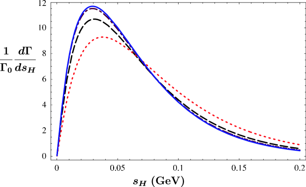
Figure 3: Plot of the kinematic corrections to the hadronic invariant mass spectrum, Eq. (58). The dashed line is the leading order result (56), while the solid line includes the full set of kinetic corrections. The dotted line corresponds to the expansion of the results of dFN to subleading order, while the dot-dashed line also includes the contribution from the $m_{b}^{5}$ term. The difference between the dot-dashed and solid curves is due to the expansion of the heavy quark spinors.

Numerically, the most important of these corrections corresponds to smearing the $m_{b}^{5}$ term, while the correction from expanding the quark fields is quite small.

However, such large corrections may be misleading, since if they are universal they may simply be absorbed in a redefinition of the leading order shape function. Instead, one should look at the corresponding relation between the hadronic invariant mass spectrum and the $\bar{B}\to X_{s}\gamma$ photon energy spectrum. One might expect that the effect of convoluting the $m_{b}^{5}$ term would cancel in the relation, since both rates are proportional to $m_{b}^{5}$. However, in the $\bar{B}\to X_{s}\gamma$ spectrum only three powers of $m_{b}$ come from the kinematics, while two arise from the factor of $m_{b}$ in the Wilson coefficient of $O_{7}$, and hence for this rate one should only convolute three powers of $m_{b}$. This may be verified by writing the results of Ref. blm01 as

$${1\over\Gamma_{0}^{s}}{d\Gamma\over dx}(\bar{B}\to X_{s}\gamma)=f(1-x)-3(1-x)f(1-x)+(1-x)f(1-x)+\dots$$ (61)

where once again the dots denote additional form factors, and the partonic rate is

$$\Gamma_{0}^{s}=\frac{G_{F}^{2}|V_{tb}V_{ts}^{*}|^{2}\alpha|C_{7}^{\mathrm{eff}}|^{2}m_{b}^{5}}{32\pi^{4}}.$$ (62)

In the expression (61), the second term corresponds to smearing three powers of $m_{b}$ in the rate, while the third third term arises from the expansion of the quark fields. Thus, there is an incomplete cancellation of the kinematic corrections between the two spectra.

IV Phenomenology

IV.1 The $\bar{B}\to X_{u}\ell\nu$ hadronic invariant mass spectrum and the $\bar{B}\to X_{s}\gamma$ photon energy spectrum

As discussed in the previous section, there are large kinematic corrections to the leading order results, largely due to the $m_{b}^{5}$ term in the rate. However, these are reduced in the relation between the hadronic invariant mass spectrum and the $\bar{B}\to X_{s}\gamma$ photon energy spectrum. Similarly, the T-product $t(x)$ is universal for all processes involving $B$ meson decays (it only differentiates between $B$ and $B^{*}$, $D$ and $D^{*}$ decays) and so its effects similarly cancel. Hence, it is useful to express the hadronic invariant mass spectrum in terms of the experimentally measurable $\bar{B}\to X_{s}\gamma$ photon energy spectrum.

The $\bar{B}\to X_{s}\gamma$ photon energy spectrum is given at tree level to subleading order in $1/m_{b}$ by blm01

$$\frac{1}{\Gamma_{0}^{s}}\frac{d\Gamma}{d\hat{E}_{\gamma}}=2F(1-2\hat{E}_{\gamma})$$ (63)

where

$$F(x)=f(x)+\left[h_{1}(x)+\frac{t(x)}{2}-2xf(x)-G_{2}(x)+H_{2}(x)\right]+\cdots.$$ (64)

(Note that at tree level only the operator $O_{7}$ contributes. At one loop, effects of other operators must be included mn01 ). Substituting this into Eq. (II.3) gives

$${1\over\Gamma_{0}}{d\Gamma\over d\hat{s}_{H}}=\int_{0}^{\infty}\;d\omega\left\{(A(\omega,\hat{s}_{H})+\delta A(\omega,\hat{s}_{H}))F(\omega-\hat{\Delta})+\delta F(\omega,\hat{s}_{H},\hat{\Delta})\right\}d\omega$$ (65)

where $A(\omega,\hat{s}_{H})$ and $\delta A(\omega,\hat{s}_{H})$ are defined in (56) and (59), and

$$\delta F(\omega,\hat{s}_{H},\hat{\Delta}) = \left[-\frac{2\hat{s}_{H}(2\hat{s}_{H}-3\omega)(\hat{s}_{H}-\omega)}{\omega^{4}}G_{2}(\omega-\hat{\Delta})\right.$$ (66)

$$\hskip 14.22636pt+\left.\frac{4\hat{s}_{H}(2\hat{s}_{H}+\omega)(\hat{s}_{H}-\omega)}{\omega^{4}}h_{1}(\omega-\hat{\Delta})\right.$$

$$\hskip 14.22636pt+\left.\frac{2\hat{s}_{H}(2\hat{s}_{H}^{2}-4\omega\hat{s}_{H}+\omega^{2})}{\omega^{4}}H_{2}(\omega-\hat{\Delta})\right]\theta(\omega-\hat{s}_{H})$$

contains the subleading shape functions. (Note that the dependence on the T-product $t(x)$ drops out of this relation.)

To extract $|V_{ub}|$, we are interested in the integrated rate

$$\Gamma_{s_{H}}(\hat{s}_{H}^{c})=\int_{0}^{\hat{s}_{H}^{c}}\frac{d\Gamma}{d\hat{s}_{H}}d\hat{s}_{H}$$ (67)

up to a maximum value $\hat{s}_{H}^{c}$. The integrated rate for $\bar{B}\to X_{u}\ell\bar{\nu}_{\ell}$ is free of backgrounds from $\bar{B}\to X_{c}\ell\bar{\nu}_{\ell}$ for $s_{H}^{c}<{m}_{D}^{2}$, although because of experimental resolution the experimental cut is typically somewhat lower: a recent BABAR measurement babarsH used $s_{H}^{c}=(1.55\,\mbox{GeV})^{2}$. From Eq. (65), we have

$$\frac{1}{\Gamma_{0}}\Gamma_{s_{H}}(\hat{s}_{H}^{c})=\int_{0}^{\infty}\left\{(\tilde{A}(\omega,\hat{s}_{H}^{c})+\delta\tilde{A}(\omega,\hat{s}_{H}^{c}))F(\omega-\hat{\Delta})+\delta\tilde{F}(\omega,\hat{s}_{H}^{c})\right\}d\omega$$ (68)

where

$$\tilde{A}(\omega,\hat{s}_{H}^{c}) = \theta(\hat{s}_{H}^{c}-\omega)+\frac{(\hat{s}_{H}^{c})^{3}(2\omega-\hat{s}_{H}^{c})}{\omega^{4}}\theta(\omega-\hat{s}_{H}^{c}),$$

$$\delta\tilde{A}(\omega,\hat{s}_{H}^{c}) = \frac{8(\hat{\Delta}-\omega)}{3}\theta(\hat{s}_{H}^{c}-\omega)+\frac{2(\hat{s}_{H}^{c})^{2}(\hat{s}_{H}^{c}(\hat{\Delta}+5\omega)-9\omega^{2})}{3\omega^{3}}\theta(\omega-\hat{s}_{H}^{c}),$$

$$\delta\tilde{F}(\omega,\hat{s}_{H}^{c}) = -\frac{2}{3}\left(G_{2}(\omega-\hat{\Delta})+2h_{1}(\omega-\hat{\Delta})+H_{2}(\omega-\hat{\Delta})\right)\theta(\hat{s}_{H}^{c}-\omega)$$ (69)

$$+\left[-\frac{(\hat{s}_{H}^{c})^{2}(3(\hat{s}_{H}^{c})^{2}-10\omega\hat{s}_{H}^{c}+9\omega^{2})}{3\omega^{4}}G_{2}(\omega-\hat{\Delta})\right.$$

$$+\frac{2(\hat{s}_{H}^{c})^{2}(3(\hat{s}_{H}^{c})^{2}-2\omega\hat{s}_{H}^{c}-3\omega^{2})}{3\omega^{4}}h_{1}(\omega-\hat{\Delta})$$

$$+\left.\frac{(\hat{s}_{H}^{c})^{2}(3(\hat{s}_{H}^{c})^{2}-8\omega\hat{s}_{H}^{c}+3\omega^{2})}{3\omega^{4}}H_{2}(\omega-\hat{\Delta})\right]\theta(\omega-\hat{s}_{H}^{c}).$$

Note that the upper limit of integration in $\omega$ corresponds to a photon energy $x_{\gamma}=1+\hat{\Delta}-\omega<0$; however, as discussed earlier, this region is outside the region of support of the shape function, and its contribution should be highly suppressed. Thus, in the relation between the spectra we may set the lower limit on $x_{\gamma}$ to zero.

Comparing the two forms for the integrated spectrum $\Gamma_{s_{H}}(\hat{s}_{H}^{c})$ in (63) and (68), we can isolate the CKM parameter $|V_{ub}|$:

$$\frac{|V_{ub}|}{|V_{tb}V_{ts}^{*}|} = \left(1-\frac{1}{2}\delta\Gamma_{s_{H}}(\hat{s}_{H}^{c})\right)\left(\frac{6\alpha|C_{7}^{\mathrm{eff}}|^{2}}{\pi}\right)^{1/2}$$ (70)

$$\times\left[\frac{\displaystyle\int_{0}^{\hat{s}_{H}^{c}}\frac{d\Gamma}{d\hat{s}_{H}}\,d\hat{s}_{H}}{\displaystyle\int^{\hat{m}_{B}/2}_{0}(\tilde{A}(\hat{m}_{B}-2\hat{E}_{\gamma},\hat{s}_{H}^{c})+\delta\tilde{A}(\hat{m}_{B}-2\hat{E}_{\gamma},\hat{s}_{H}^{c}))\frac{d\Gamma}{d\hat{E}_{\gamma}}d\hat{E}_{\gamma}}\right]^{1/2}$$

where we have defined

$$\delta\Gamma_{s_{H}}(\hat{s}_{H}^{c})={\displaystyle\int_{0}^{\infty}\delta\tilde{F}(\omega,\hat{s}_{H}^{c})\;d\omega\over\displaystyle\int_{0}^{\infty}\tilde{A}(\omega,\hat{s}_{H}^{c})f(\omega-\hat{\Delta})\;d\omega}$$ (71)

which contains the effects of the new subleading distribution functions. For comparison purposes, we also define

$$\delta\Gamma_{s_{H}}^{\rm full}(\hat{s}_{H}^{c})={\displaystyle\int_{0}^{\infty}\delta\tilde{A}(\omega,\hat{s}_{H}^{c})f(\omega-\hat{\Delta})+\delta\tilde{F}(\omega,\hat{s}_{H}^{c})\;d\omega\over\displaystyle\int_{0}^{\infty}\tilde{A}(\omega,\hat{s}_{H}^{c})f(\omega-\hat{\Delta})\;d\omega}$$ (72)

which gives the full fractional subleading correction to the relation between the two spectra. To proceed further we must introduce a model for the shape functions.

IV.2 Shape function models

The shape functions are nonperturbative functions which cannot at present be calculated from first principles. We do, however, know several moments of these functions blm01 , and we can use this information to constrain possible models of the shape functions.

The leading order shape function is modeled with $f_{\mathrm{mod}}(\omega)$ defined in (60). We will use three models of the subleading shape functions. The first was introduced in blm01 , based on the leading order function $f_{\mathrm{mod}}(\omega)$. The subleading functions are defined as

$$h_{1\;\mathrm{mod1}}(\omega) = \frac{\lambda_{2}}{m_{b}^{2}}f^{\prime}_{\mathrm{mod}}(\omega)$$

$$G_{2\;\mathrm{mod1}}(\omega) = -\frac{2\lambda_{1}}{3m_{b}^{2}}f^{\prime}_{\mathrm{mod}}(\omega)$$

$$H_{2\;\mathrm{mod1}}(\omega) = -\frac{\lambda_{2}}{m_{b}^{2}}f^{\prime}_{\mathrm{mod}}(\omega)$$

$$t_{\mathrm{mod1}}(\omega) = -\frac{\lambda_{1}+3\lambda_{2}}{m_{b}^{2}}f^{\prime}_{\mathrm{mod}}(\omega)$$ (73)

to reproduce the leading terms in Eq. (II.3).

The second model was introduced in mn02 , in which the subleading functions are defined in terms of a single function

$$s(\omega,b)=-\frac{b^{2}}{\hat{\Delta}^{2}}e^{-b(1+\omega/\hat{\Delta})}\left(b(1+\omega/\hat{\Delta})-1\right)\theta(1+\omega/\hat{\Delta}).$$ (74)

The dimensionless free parameter $b$ is constrained to be ${\cal O}(1)$ by the requirement that the $n$th moments of the functions scale like $\hat{\Delta}^{n+1}$. We will take $b=1$ in our plots; larger values of $b$ reduce the effects of the subleading shape functions. We have

$$h_{1\;\mathrm{mod2}}(\omega,b) = \frac{\lambda_{2}}{m_{b}^{2}}s(\omega,b)$$

$$G_{2\;\mathrm{mod2}}(\omega,b) = -\frac{2\lambda_{1}}{3m_{b}^{2}}s(\omega,b)$$

$$H_{2\;\mathrm{mod2}}(\omega,b) = -\frac{\lambda_{2}}{m_{b}^{2}}s(\omega,b).$$

$$t_{\mathrm{mod2}}(\omega,b) = -\frac{(\lambda_{1}+3\lambda_{2})}{m_{b}^{2}}s(\omega,b).$$ (75)

Note that in the first model the subleading shape functions vanish at $\omega=\hat{\Delta}$, while in the second they are finite but nonzero.

In our third model, we use a model for the subleading shape functions that has an additional sign flip in the region of integration. We take

$$h_{1\;\mathrm{mod3}}(\omega) = \frac{\lambda_{2}}{m_{b}^{2}}f^{\prime}_{2}(\omega)$$

$$G_{2\;\mathrm{mod3}}(\omega) = -\frac{2\lambda_{1}}{3m_{b}^{2}}f^{\prime}_{2}(\omega)$$

$$H_{2\;\mathrm{mod3}}(\omega) = -\frac{\lambda_{2}}{m_{b}^{2}}f^{\prime}_{2}(\omega)$$

$$t_{\mathrm{mod3}}(\omega) = -\frac{(\lambda_{1}+3\lambda_{2})}{m_{b}^{2}}f^{\prime}_{2}(\omega)$$ (76)

where

$$f_{2}(\omega)=-\frac{32}{\pi^{2}\hat{\Delta}}\left(\omega+\hat{\Delta}\right)\theta\left(1+\frac{\omega}{\hat{\Delta}}\right){d\over d\omega}\left(\left(1+\frac{\omega}{\hat{\Delta}}\right)^{3}e^{-\frac{4}{\pi}(1+\omega/\hat{\Delta})^{2}}\right).$$ (77)

We plot the function $h_{1}(\omega)$ in each of these models in Fig. 4.

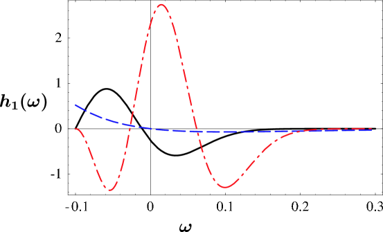
Figure 4: Three models of $h_{1}(\omega)$: model 1 (solid curve), model 2 (dashed curve) and model 3 (dot-dashed curve).

Although the models have very different behaviour, we can verify that they are all reasonable by calculating the first few moments ${\cal M}_{n}\equiv\int_{-\infty}^{\infty}\omega^{n}H_{2}(\omega)d\omega$ in each model and showing that they are of order $(\Lambda_{\rm QCD}/m_{b})^{n+1}$. For $m_{b}=4.8$ GeV, for model 1 we find $|{\cal M}_{1}|=(0.35\,{\rm GeV}/m_{b})^{2},|{\cal M}_{2}|=0,\ |{\cal M}_{3}|=(0.35\,{\rm GeV}/m_{b})^{4}$ and $|{\cal M}_{4}|=(0.29\,{\rm GeV}/m_{b})^{5}$. For model 2 we find $|{\cal M}_{1}|=(0.35\,{\rm GeV}/m_{b})^{2},|{\cal M}_{2}|=(0.49\,{\rm GeV}/m_{b})^{3},\ |{\cal M}_{3}|=(0.70\,{\rm GeV}/m_{b})^{4}$ and $|{\cal M}_{4}|=(0.90\,{\rm GeV}/m_{b})^{5}$, while for model 3 the corresponding moments are $|{\cal M}_{1}|=(0.35\,{\rm GeV}/m_{b})^{2},\ |{\cal M}_{2}|=(0.54\,{\rm GeV}/m_{b})^{3},\ |{\cal M}_{3}|=(0.54\,{\rm GeV}/m_{b})^{4}$ and $|{\cal M}_{4}|=(0.58\,{\rm GeV}/m_{b})^{5}$. Thus, the first few moments of each model scale like typical hadronic scales to the appropriate power. Similar results are obtained for the moments of $G_{2}(\omega)$ and $h_{1}(\omega)$.

IV.3 Numerical results

Both the Wilson coefficients and models for the shape functions depend on the $b$ quark mass $m_{b}$. While in our formulas we are implicitly using the pole mass, it is well-known that this leads to badly behaved perturbative series, and so we expect that radiative corrections to these results will be minimized if a sensible short-distance mass is used instead. The $\overline{\mbox{MS}}$ mass $\bar{m}_{b}(\bar{m}_{b})$ is well-defined, but does not lead to small perturbative corrections in $B$ decays lsw95 ; bsuv96 . The “threshold” masses, including the 1S mass, PS mass and kinetic mass, are preferable in this context. At two-loops, a pole mass of $m_{b}=4.8$ GeV corresponds to a kinetic mass $m_{b}^{\rm kin}(1\,\mbox{GeV})$ of about 4.6 GeV, PS and 1S masses of about $4.7\,\mbox{GeV}$ and an $\overline{\mbox{MS}}$ mass $\bar{m}_{b}(\bar{m}_{b})$ of about 4.3 GeV. Thus, to give an estimate of the $m_{b}$ dependence of our results, we plot them for $m_{b}=4.8$ GeV and $m_{b}=4.5$ GeV.

In Fig. 5, we plot the hadronic invariant mass spectrum using the three models of the previous section for the subleading corrections. These corrections are clearly large and model dependent over much of the spectrum.

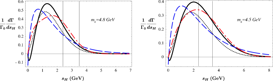
Figure 5: Model calculations of the hadronic invariant mass spectrum $d\Gamma/ds_{H}$, for $m_{b}=4.8\,\mbox{GeV}$ (a) and $m_{b}=4.5\,\mbox{GeV}$ (b). The dotted curve is the leading order result; the other curves are the results in the models discussed in the text. The curves are denoted as in Fig. 4. The right vertical line denotes the kinematic limit $s_{H}=m_{D}^{2}$; the left line denotes the BABAR cut $s_{H}=(1.55\,\mbox{GeV})^{2}$.

However, the integrated rate is much less sensitive to the subleading corrections. The functions $\delta\Gamma_{s_{H}}(\hat{s}_{H}^{c})$ and $\delta\Gamma_{s_{H}}^{\rm full}(\hat{s}_{H}^{c})$ defined in Eqs. (71) and (72) are plotted in Fig. 6 for the three models presented in the previous section.

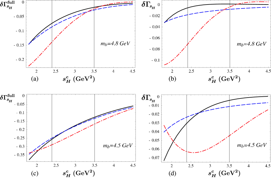
Figure 6: Model calculations of the fractional corrections $\delta\Gamma_{s_{H}}^{\rm full}$ and $\delta\Gamma_{s_{H}}$ to the cut width, as defined in Eqs. (71) and (72), for $m_{b}=4.8\,\mbox{GeV}$ (a,b) and $m_{b}=4.5\,\mbox{GeV}$ (c,d). The three curves refer to the three different models in Fig. 4. $\delta\Gamma_{s_{H}}^{\rm full}$ includes all the subleading corrections, including those proportional to the leading order shape function, while $\delta\Gamma_{s_{H}}$ only includes the corrections from subleading shape functions. The right vertical line denotes the kinematic limit $s_{H}=m_{D}^{2}$; the left line denotes the BABAR cut $s_{H}=(1.55\,\mbox{GeV})^{2}$.

From these figures it is clear that, at least for the particular models we have chosen, the subleading shape functions do not contribute a large uncertainty in the extraction of $|V_{ub}|$, and that the dominant subleading effects are from the kinematic terms. This should not be surprising: since there are no $O(\Lambda_{\rm QCD}/m_{b})$ corrections to the total semileptonic decay rate operefs , the subleading corrections must vanish when integrated over the full spectrum. Since the experimental cuts include a large fraction of the rate, the contribution to the integrated rate from the subleading corrections is correspondingly suppressed. This is evident from the plots in Fig. 6, where the fractional correction tends to zero as the cut is increased.

It is useful to compare these results with analogous results for the lepton energy spectrum in semileptonic $B$ decays, given in blm02 . In this case, only $\sim 10\%$ of the rate is included, and the subleading corrections are substantial. The analogous relation to Eq. (70) is

$$\frac{|V_{ub}|}{|V_{tb}V_{ts}^{*}|}=\left(1-\frac{1}{2}\delta\Gamma_{E_{\ell}}(\hat{E}_{\ell}^{c})\right)\left(\frac{6\alpha|C_{7}^{\mathrm{eff}}|^{2}}{\pi}\right)^{1/2}\left[\frac{\int_{\hat{E}_{\ell}^{c}}^{\hat{m}_{B}/2}\frac{d\Gamma}{d\hat{E}_{\ell}}\,d\hat{E}_{\ell}}{\int_{\hat{E}_{\ell}^{c}}^{\hat{m}_{B}/2}8(\hat{E}_{\gamma}-\hat{E}_{\ell}^{c})(1-\hat{E}_{\gamma})\frac{d\Gamma}{d\hat{E}_{\gamma}}\,d\hat{E}_{\gamma}}\right]^{1/2}$$ (78)

where

$$\delta\Gamma_{E_{\ell}}(\hat{E}_{\ell}^{c})=2\frac{\int_{0}^{\hat{m}_{B}-2\hat{E}_{\ell}^{c}}(\hat{m}_{B}-2\hat{E}_{\ell}^{c}-\omega)(H_{2}(\omega-\hat{\Delta})-h_{1}(\omega-\hat{\Delta}))\,d\omega}{\int_{0}^{\hat{m}_{B}-2\hat{E}_{\ell}^{c}}(\hat{m}_{B}-2\hat{E}_{\ell}^{c}-\omega)f(\omega-\hat{\Delta})\,d\omega}.$$ (79)

In Fig. 7 we plot $\delta\Gamma_{E_{\ell}}(E_{\ell})$ for $m_{b}=4.8\ \mbox{GeV}$ and $m_{b}=4.5\ \mbox{GeV}$ in the three models used in this paper. It is clear from the figures that for lepton cuts near the kinematic limit $E_{\ell}=2.3$ GeV, the uncertainty in $|V_{ub}|$ from higher order shape functions is much greater for the lepton energy spectrum than from the hadronic invariant mass spectrum.

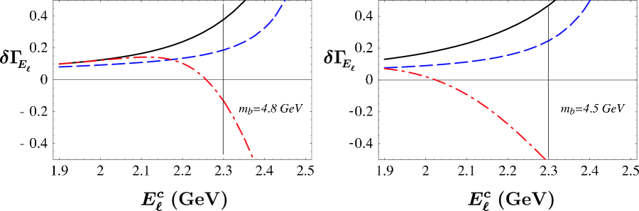
Figure 7: Model calculations of the fractional corrections $\delta\Gamma_{E_{\ell}}$ for the semileptonic $B\to X_{u}$ decay width with a charged lepton energy cut, as defined in Eq. (79). The three curves refer to the three different models in Fig. 4. The solid line denotes the kinematic upper limit from $B\to X_{c}$ decay.

V Conclusions

We have calculated the hadronic invariant mass spectrum for $\bar{B}\to X_{u}\ell\bar{\nu}_{\ell}$ in terms of shape functions to subleading order. Introducing some simple models for the shape functions we have studied the $d\Gamma/ds_{H}$ spectrum numerically.

Since we know little about the form of the subleading shape functions, it is difficult to estimate the corresponding theoretical uncertainty in $|V_{ub}|$. However, using the spread of models as a guide, we can conclude that the largest subleading effects are proportional to the leading order shape function, and so, given a determination of the shape function from $\bar{B}\to X_{s}\gamma$ decay, do not increase the theoretical uncertainty. Assuming our spread of models provides a reasonable measure of the theoretical uncertainty, we can conclude that the theoretical uncertainty in $|V_{ub}|$ due to higher order shape functions is at the few percent level. This is substantially less than the corresponding uncertainty in the integrated lepton energy spectrum with the current experimental cuts. This is also much less than the other sources of experimental and theoretical error in the current measurements of the integrated hadronic energy spectrum.

- (1) J. Chay, H. Georgi, and B. Grinstein, Phys. Lett. B247 (1990) 399; M. Voloshin and M. Shifman, Sov. J. Nucl. Phys. 41 (1985) 120; I.I. Bigi et al., Phys. Lett. B293 (1992) 430; Phys. Lett B297 (1993) 477 (E); I.I. Bigi et al., Phys. Rev. Lett. 71 (1993) 496; A.V. Manohar and M.B. Wise, Phys. Rev. D49 (1994) 1310; B. Blok et al., Phys. Rev. D49 (1994) 3356; A. F. Falk, M. Luke and M. J. Savage, Phys. Rev. D 49, 3367 (1994).
- (2) R. A. Briere et al. [CLEO Collaboration], arXiv:hep-ex/0209024.
- (3) A. H. Hoang, Z. Ligeti and A. V. Manohar, Phys. Rev. Lett. 82, 277 (1999); ibid., Phys. Rev. D 59, 074017 (1999);
- (4) A. H. Hoang and T. Teubner, Phys. Rev. D 60, 114027 (1999).
- (5) A. F. Falk, M. E. Luke and M. J. Savage, Phys. Rev. D 53, 2491 (1996). Phys. Rev. D 53, 6316 (1996); A. F. Falk and M. E. Luke, Phys. Rev. D 57, 424 (1998).
- (6) A. Kapustin and Z. Ligeti, Phys. Lett. B355 (1995) 318; C. Bauer, Phys. Rev. D57 (1998) 5611; Erratum ibid. D60 (1999) 099907; Z. Ligeti, M. Luke, A.V. Manohar, and M.B. Wise, Phys. Rev. D60 (1999) 034019; D. Cronin-Hennessy et al. [CLEO Collaboration], Phys. Rev. Lett. 87, 251808 (2001); R. A. Briere et al. [CLEO Collaboration], arXiv:hep-ex/0209024; B. Aubert et al. (BABAR Collaboration), hep-ex/0207084; DELPHI Collaboration, Contributed paper for ICHEP 2002, 2002-070-CONF-605; 2002-071-CONF-604; C. W. Bauer, Z. Ligeti, M. Luke and A. V. Manohar, Phys. Rev. D 67, 054012 (2003).
- (7) N. Uraltsev, Int. J. Mod. Phys. A14 (1999) 4641.
- (8) V. Barger, C. S. Kim and R. J. Phillips, Phys. Lett. B251, (1990) 629; A.F. Falk, Z. Ligeti, and M.B. Wise, Phys. Lett. B406 (1997) 225; I. Bigi, R.D. Dikeman, and N. Uraltsev, Eur. Phys. J. C4 (1998) 453; R. D. Dikeman and N. Uraltsev, Nucl. Phys. B509 (1998) 378; P. Abreu et al. [DELPHI Collaboration], Phys. Lett. B478 (2000) 14.
- (9) C.W. Bauer, Z. Ligeti, and M. Luke, Phys. Lett. B479 (2000) 395; M. Neubert, JHEP 0007 (2000) 022.
- (10) C. W. Bauer, Z. Ligeti and M. Luke, Phys. Rev. D64 (2001) 113004.
- (11) F. De Fazio and M. Neubert, JHEP06 (1999) 017.
- (12) M. Neubert, Phys. Rev. D49 (1994) 3392; D49 (1994) 4623; I.I. Bigi et al., Int. J. Mod. Phys. A9 (1994) 2467.
- (13) T. Mannel and M. Neubert, Phys. Rev. D50 (1994) 2037.
- (14) G. P. Korchemsky and G. Sterman, Phys. Lett. B 340, 96 (1994); R. Akhoury and I. Z. Rothstein, Phys. Rev. D 54, 2349 (1996); A. K. Leibovich and I. Z. Rothstein, Phys. Rev. D 61, 074006 (2000); A. K. Leibovich, I. Low and I. Z. Rothstein, Phys. Rev. D 61, 053006 (2000); A. K. Leibovich, I. Low and I. Z. Rothstein, Phys. Rev. D 62, 014010 (2000); A. K. Leibovich, I. Low and I. Z. Rothstein, Phys. Lett. B 486, 86 (2000).
- (15) C. W. Bauer and A. V. Manohar, arXiv:hep-ph/0312109.
- (16) C. W. Bauer, M. E. Luke and T. Mannel, arXiv:hep-ph/0102089.
- (17) C. W. Bauer, M. Luke and T. Mannel, Phys. Lett. B543 (2002) 261.
- (18) M. Neubert, Phys. Lett. B 543 (2002) 269.
- (19) A. K. Leibovich, Z. Ligeti and M. B. Wise, Phys. Lett. B539 (2002) 242.
- (20) M. Gremm and A. Kapustin, Phys. Rev. D 55, 6924 (1997).
- (21) M. Neubert, Phys. Lett. B 513, 88 (2001)
- (22) B. Aubert et al. [BABAR Collaboration], arXiv:hep-ex/0307062.
- (23) M. E. Luke, M. J. Savage and M. B. Wise, Phys. Lett. B 343, 329 (1995); Phys. Lett. B 345, 301 (1995).
- (24) I. I. Y. Bigi, M. A. Shifman, N. Uraltsev and A. I. Vainshtein, Phys. Rev. D 56, 4017 (1997).