Bounds on $\gamma$ from CP violation measurements in $B\rightarrow\pi^{+}\pi^{-}$ and $B\rightarrow\psi K_{S}$

Abstract

We study the determination of $\gamma$ from CP-violating observables in $B\rightarrow\pi^{+}\pi^{-}$ and $B\rightarrow\psi K_{S}$. This determination requires theoretical input to one combination of hadronic parameters. We show that a mild assumption about this quantity may allow bounds to be placed on $\gamma$, but we stress the pernicious effects that an eightfold discrete ambiguity has on such an analysis. The bounds are discussed as a function of the direct ($C$) and interference ($S$) CP-violating observables obtained from time-dependent $B\rightarrow\pi^{+}\pi^{-}$ decays, and their behavior in the presence of new physics effects in $B-\overline{B}$ mixing is studied.

I Introduction

The Standard Model (SM) of electroweak interactions has been so successful that increasingly detailed probes are required in order to uncover possible new physics effects. CP violation seems to provide a particularly promising probe, because it appears in the SM through one single irremovable phase in the Cabibbo-Kobayashi-Maskawa (CKM) matrix CKM . As a result, the measurements of any two CP-violating experiments must be related through CP-conserving quantities. In principle, this makes the SM a very predictive theory of CP violation. In practice, however, the CP-conserving quantities required to extract weak interaction parameters from experiment usually involve the strong interaction, are difficult to calculate, and the interpretations of the experiments in terms of parameters of the original Lagrangian are plagued by hadronic uncertainties.

One notable exception occurs with the determination of $\sin{(2\tilde{\beta})}$ from the time dependent asymmetry in $B\rightarrow\psi K_{S}$. In the SM, and with the usual phase convention, $\tilde{\beta}\equiv\beta$ is the phase of $V_{td}^{\ast}$. The current world average is Browder

$$\sin{(2\tilde{\beta})}=0.736\pm 0.049,$$ (1)

based on the very precise measurements by Babar Babar and Belle Belle . In this article, we will also consider the possibility that there might be new physics contributions affecting the phase of $B-\overline{B}$ mixing note-magnitude-BBbar . In that case, the phase $\tilde{\beta}$ measured in $B\rightarrow\psi K_{S}$ decays does not coincide with the phase $\beta$ of $V_{td}^{\ast}$.

The current measurement of $\beta$ is in agreement with measurements based on $|V_{ub}/V_{cb}|$, $\Delta m_{B}$, $\Delta m_{Bs}$, and CP violation in the $K-\overline{K}$ system, although each of these is plagued by hadronic uncertainties.

So, we would like to constrain the CKM source of CP violation in as many ways as possible, in the hope of uncovering new physics effects. One possibility arises in the time-dependent asymmetry in $B\rightarrow\pi^{+}\pi^{-}$ decays. If there were only contributions from tree level diagrams, this would provide a clean measurement of $\sin{(2\tilde{\beta}+2\gamma)}$ BLS . Unfortunately, the presence of penguin contributions with a different weak phase imply that this measurement is plagued by hadronic uncertainties. One way out of this problem consists in estimating this penguin pollution in some way (see section II). Recently, Buchalla and Safir (BS) have proposed a different approach BS . In their method, a mild assumption is made about the needed theoretical input in order to derive a bound on $\gamma$, which is valid provided the interference CP violation observable in $B\rightarrow\pi^{+}\pi^{-}$ (S) lies above $-\sin{(2\tilde{\beta})}$. Their bound holds within the SM (although this is not obvious from their article) and can be obtained in the limit of no penguin pollution that corresponds to setting the direct CP violation observable in $B\rightarrow\pi^{+}\pi^{-}$ (C) to zero.

In this article, we extend their result by studying which bounds occur when $C\neq 0$ and when there are new physics in $B-\overline{B}$ mixing (that is, when $\tilde{\beta}\neq\beta$). Because we do not go through the Wolfenstein’s parameters $\rho$ and $\eta$ Wolf , we obtain, as a particular case, an easier derivation of the BS result. Our analysis will allow us to state what types of new physics effects are subject to these new bounds and how they change from $C=0$ to $C\neq 0$. In particular, we will stress the very important impact that an eightfold discrete ambiguity has on such bounds.

Although that is not the main point of this article, we will also comment briefly on how one can perform the precise determination of $\gamma$, once a specific value for the relevant hadronic quantity is taken. In doing so, we differ from previous analysis in that we start from the experimental values for $C$ and $S$ (using only the one piece of theoretical input required) rather than plot “predictions” for $C$ and $S$ given a number of theoretical inputs. The end result is the same, but this is closer in spirit to what one really wishes to do; we wish to use experimental results in order to learn about theoretical parameters and not the converse.

Our article is organized as follows. In section II, we set the notation, introducing the relevant experimental and theoretical quantities involved in $B\rightarrow\pi^{+}\pi^{-}$ decays. In section III we develop the two formulas which will guide our analysis of the bounds on $\gamma$ discussed in section IV. We draw our conclusions in section V and include a trivial but useful inequality in the appendix.

II Experimental observables versus Theoretical parameters

The time-dependent CP asymmetry in $B\rightarrow\pi^{+}\pi^{-}$ decays may be written asBLS

$$A_{CP}(t) = \frac{\Gamma[B(t)\rightarrow\pi^{+}\pi^{-}]-\Gamma[\overline{B}(t)\rightarrow\pi^{+}\pi^{-}]}{\Gamma[B(t)\rightarrow\pi^{+}\pi^{-}]+\Gamma[\overline{B}(t)\rightarrow\pi^{+}\pi^{-}]}$$ (2)

$$= -S\sin{\Delta m_{B}\,t}+C\cos{\Delta m_{B}\,t},$$

where

$$S=\frac{2{\textrm{I}m}\lambda}{1+|\lambda|^{2}}\ \ \ \ \ \ \ \ C=\frac{1-|\lambda|^{2}}{1+|\lambda|^{2}}.$$ (3)

Clearly $S^{2}+C^{2}\leq 1$. The corresponding experimental results are Babar-pipi ; BELLE-pipi

$$S = \left\{\begin{array}[]{ll}-0.40\pm 0.22\pm 0.03&(\textrm{Babar})\\ -1.23\pm 0.41^{+0.08}_{-0.07}&(\textrm{Belle})\end{array}\right.$$ (6)

$$C = \left\{\begin{array}[]{ll}-0.19\pm 0.19\pm 0.05&(\textrm{Babar})\\ -0.77\pm 0.27\pm 0.08&(\textrm{Belle})\end{array}\right.$$ (9)

which the Heavy Flavour Averaging Group combines into $S=-0.58\pm 0.20$ and $C=-0.38\pm 0.16$ HFAG . Eqs. (3) and (9) imply that $\lambda$ is a quantity accessible experimentally, up to a twofold discrete ambiguity Dun95 in its real part:

$$\pm\sqrt{1-C^{2}-S^{2}}=\frac{2{\textrm{R}e}\lambda}{1+|\lambda|^{2}}.$$ (10)

On the other hand, $\lambda$ may be written in terms of theoretical parameters as

$$\lambda=\frac{q}{p}\frac{\bar{A}}{A},$$ (11)

where $q/p$ reflects the $B-\overline{B}$ mixing, and $A$ ($\bar{A}$) is the amplitude for the $B\rightarrow\pi^{+}\pi^{-}$ ($\overline{B}\rightarrow\pi^{+}\pi^{-}$) decay. With the usual phase convention for the CKM parameters, these quantities may be written in terms of weak and strong interaction parameters as

$$\frac{q}{p} = e^{-2i\tilde{\beta}},$$

$$A=V_{ub}^{\ast}V_{ud}\,T+V_{cb}^{\ast}V_{cd}\,P\,e^{i\delta} = |V_{ub}V_{ud}\,T|\left(e^{i\gamma}+z\right),$$

$$\bar{A}=V_{ub}V_{ud}^{\ast}\,T+V_{cb}V_{cd}^{\ast}P\,e^{i\delta} = |V_{ub}V_{ud}\,T|\left(e^{-i\gamma}+z\right),$$ (12)

where $P$ and $T$ are magnitudes of hadronic quantities, $\delta$ is a strong phase difference, and

$$z=\frac{P/T}{R_{b}}e^{i\delta}=re^{i\delta}$$ (13)

includes a dependence on the weak parameter $R_{b}=|V_{ub}V_{ud}|/|V_{cb}V_{cd}|=\sqrt{\rho^{2}+\eta^{2}}$. The weak phase $\tilde{\beta}$ coincides with the CKM parameter $\beta$, if one stays within the framework of the SM; but $\tilde{\beta}$ may differ from $\beta$, if there are new physics contributions affecting the phase in $B-\overline{B}$ mixing note-magnitude-BBbar .

Substituting Eqs. (12) in Eq. (11), we obtain

$$\lambda=e^{-2i\tilde{\beta}}\ \frac{e^{-i\gamma}+z}{e^{i\gamma}+z}.$$ (14)

This equation relates the measurable quantity on the LHS with the theoretical quantities on the RHS. In some sense, these two sides are usually kept apart. (As we shall see in section III, great simplifications occur if we subvert this standard practice.) One may now substitute Eq. (14) in Eqs. (3) to find note2

$$S = -\frac{\sin{(2\tilde{\beta}+2\gamma)}+2r\sin{(2\tilde{\beta}+\gamma)}\cos{\delta}+r^{2}\sin{(2\tilde{\beta})}}{1+2r\cos{\gamma}\cos{\delta}+r^{2}},$$ (15)

$$C = \frac{2r\sin{\gamma}\sin{\delta}}{1+2r\cos{\gamma}\cos{\delta}+r^{2}},$$ (16)

$$\frac{2{\textrm{R}e}\lambda}{1+|\lambda|^{2}} = \frac{\cos{(2\tilde{\beta}+2\gamma)}+2r\cos{(2\tilde{\beta}+\gamma)}\cos{\delta}+r^{2}\cos{(2\tilde{\beta})}}{1+2r\cos{\gamma}\cos{\delta}+r^{2}}.$$ (17)

If there were no penguin amplitudes ($r=0$), then $\lambda$ would be given by the pure phase $-2\tilde{\beta}-2\gamma$, which is by definition equal do $2\alpha$ (mod.  $2\pi$). In that case, $C$ would vanish and $S$ would provide a clear determination of the phase $\tilde{\beta}+\gamma$, which in the SM coincides with $\beta+\gamma$. As is well know, the presence of the “penguin pollution” spoils this determination. In fact, since $\tilde{\beta}$ has been determined in $B\rightarrow\psi K_{S}$ decays, there are two experimental observables ($C$ and $S$) and three unknowns ($r$, $\delta$, and the weak phase $\gamma$). One needs some extra piece of information about the hadronic parameters $r$ and $\delta$ in order to determine the weak phase $\gamma$.

This extra information may be achieved in a variety of ways. Gronau and London GL used isospin to relate $B\rightarrow\pi^{+}\pi^{-},\pi^{0}\pi^{0}$ and $B^{+}\rightarrow\pi^{+}\pi^{0}$ decays. Their method has received renewed life from the recent announcements by Babar Babar-pi0pi0 and Belle BELLE-pi0pi0 of a large branching ratio for the $\pi^{0}\pi^{0}$ final state. Silva and Wolfenstein SW94 proposed an estimate of the penguin contribution through an SU(3) relation between $B\rightarrow\pi^{+}\pi^{-}$ and $B\rightarrow K^{+}\pi^{-}$. Chiang, Gronau and Rosner CGR used SU(3) to estimate P/T from a variety of observables. Alternatively, one may estimate $r$ and $\delta$ directly from theory, within QCD factorization BBNS ; Buchalla and Safir quote $rR_{b}=0.107\pm 0.031$ and $\delta=0.15\pm 0.25$ BS .

One could try to proceed without the extra piece of information. Working within the SM, one could substitute $\tilde{\beta}=\beta$ and $\gamma$ by $\rho$ and $\eta$ on the RHS of Eq. (15), which would lead to a rather complicated expression. (Notice that this substitution is only possible within the SM, since, in general, $\tilde{\beta}$ is not related to $\rho$ and $\eta$.) Such work has been done recently by Buchalla and Safir BS , who point out that a lower bound on $\eta$ (and, thus, $\gamma$) can be achieved with a mild assumption on the hadronic parameters, as long as $S>-\sin{(2\beta)}$. The value of that lower bound is equal to the value that one would obtain for $\eta$ ($\gamma$) in the limit of vanishing penguin amplitude (that is, with C=0). In what follows, we will recover their result in a much simpler way, by evading any mention of $\rho$ and $\eta$. This will allow us to generalize their result for $C\neq 0$ and to discuss how such bounds are affected by possible new physics contributions to the $B-\overline{B}$ mixing phase.

III Two master formulae

We start from Eq. (14), and multiply both sides by the denominator of the RHS. Reordering the terms, we obtain

$$\lambda e^{i\gamma}-e^{-2i\tilde{\beta}}e^{-i\gamma}=z(e^{-2i\tilde{\beta}}-\lambda).$$ (18)

Equating the real and imaginary parts

$$\textrm{Re}(\lambda-e^{-2i\tilde{\beta}})\cos{\gamma}-\textrm{Im}(\lambda+e^{-2i\tilde{\beta}})\sin{\gamma} = \textrm{Re}\left[z(e^{-2i\tilde{\beta}}-\lambda)\right],$$

$$\textrm{Im}(\lambda-e^{-2i\tilde{\beta}})\cos{\gamma}+\textrm{Re}(\lambda+e^{-2i\tilde{\beta}})\sin{\gamma} = \textrm{Im}\left[z(e^{-2i\tilde{\beta}}-\lambda)\right],$$ (19)

we find

$$\cos{\gamma} = -\textrm{Re}(z)-\frac{2\,\textrm{Im}(\lambda e^{2i\tilde{\beta}})}{1-|\lambda|^{2}}\,\textrm{Im}(z),$$

$$\sin{\gamma} = \frac{(1+|\lambda|^{2})-2\,\textrm{Re}(\lambda e^{2i\tilde{\beta}})}{1-|\lambda|^{2}}\,\textrm{Im}(z).$$ (20)

Using Eqs. (3) and (10), we may rewrite Eqs. (20) as

$$\cos{\gamma_{\pm}} = -\textrm{Re}(z)-\frac{I_{\pm}}{C}\,\textrm{Im}(z),$$

$$\sin{\gamma_{\pm}} = \frac{1-R_{\pm}}{C}\,\textrm{Im}(z),$$ (21)

where

$$R_{\pm} = \frac{2\,\textrm{Re}(\lambda e^{2i\tilde{\beta}})}{1+|\lambda|^{2}}=\pm\sqrt{1-C^{2}-S^{2}}\cos{(2\tilde{\beta})}-S\sin{(2\tilde{\beta})},$$

$$I_{\pm} = \frac{2\,\textrm{Im}(\lambda e^{2i\tilde{\beta}})}{1+|\lambda|^{2}}=S\cos{(2\tilde{\beta})}\pm\sqrt{1-C^{2}-S^{2}}\sin{(2\tilde{\beta})},$$ (22)

are determined exclusively from experiment, with the discrete ambiguity present in Eq. (10). It is easy to show (c.f. the appendix) that $|R_{\pm}|$ and $|I_{\pm}|$ are bounded by $\sqrt{1-C^{2}}$.

Eqs. (21) depend on two different combinations of hadronic parameters, which we may choose as $\{\textrm{Re}(z),\textrm{Im}(z)\}$ or as $\{r,\delta\}$. As we know from the parameter counting of the previous section, one combination of hadronic parameters will always remain. The other combination may be eliminated in a variety of ways. For example,

$$\tan{\gamma_{\pm}}=\frac{-1+R_{\pm}}{C\cot{\delta}+I_{\pm}},$$ (23)

or

$$I_{\pm}\sin{\gamma_{\pm}}+(1-R_{\pm})(\cos{\gamma_{\pm}}+Q)=0,$$ (24)

with

$$Q=r\cos{\delta}$$ (25)

A few comments are in order. First, Eq. (23) has a form which will allow us to derive a bound on $\gamma$ which generalizes the results of BS in a very clear way. Second, for a given set of experimental values for $\sin{(2\tilde{\beta})}$, $C$, and $S$, the theoretical parameter $\delta$ cannot take an arbitrary value. For example, if $C\neq 0$ then $\delta$ cannot vanish, as is easily seen from Eq. (16). Third, we have found numerically that, even if one takes a value of $\delta$ consistent with the experimental observables, Eq. (23) is very sensitive to the exact value chosen for $\delta$. For the previous reasons, and although Eq. (23) is so well suited to study the bounds on $\gamma$, Eq. (24) is more useful when studying the dependence of $\gamma$ on the theoretical parameters (through $Q$). Finally, for a given set of experimental values of $\sin{(2\tilde{\beta})}$, $C$, and $S$, and for the same $\cot{\delta}$, there is an eightfold ambiguity in the determination of $\gamma$. A twofold ambiguity arises from the existence of two values of $\tan{\gamma}$ ($\tan{\gamma_{+}}$ and $\tan{\gamma_{-}}$) which satisfy Eq. (23). This is related to the ${\textrm{R}e}\lambda$ in Eq. (10), whose measurement would remove this twofold ambiguity, and implies that $\lambda_{+}=-\lambda_{-}^{\ast}$. Of course, this is obtained for different values of $r$. Another twofold ambiguity arises from the unknown sign of $\cos{(2\tilde{\beta})}$. The compound transformation $\cos{(2\tilde{\beta})}\rightarrow-\cos{(2\tilde{\beta})}$ and $\cot{\delta}\rightarrow-\cot{\delta}$ leads to $\tan{\gamma_{\pm}}\rightarrow-\tan{\gamma_{\mp}}$. The final twofold ambiguity arises from the inversion of the function $\tan{\gamma}$, and corresponds to a symmetry $\gamma\rightarrow\pi+\gamma$. If there is no new physics in the $K-\overline{K}$ system, and if we trust the sign of the bag parameter, then this ambiguity is removed since $\gamma$ cannot lie outside $(0,\pi)$.

In the next section, we will use Eqs. (23) and (24) together with mild assumptions on the hadronic parameters $\delta$ and $Q$ (respectively), in order to provide model independent bounds on the CKM phase $\gamma$.

IV Bounds on $\gamma$

IV.1 Bounds on $\tan{\gamma_{\pm}}$

We will now study Eq. (23) in more detail. Every quantity on the RHS of that equation is determined from experiment, aside from $\cot{\delta}$. It would be nice to be able to relate $\tan{\gamma_{\pm}}$ to the value

$$L_{\pm}=\frac{-1+R_{\pm}}{I_{\pm}}=\frac{-1\pm\sqrt{1-C^{2}-S^{2}}\cos{(2\tilde{\beta})}-S\sin{(2\tilde{\beta})}}{S\cos{(2\tilde{\beta})}\pm\sqrt{1-C^{2}-S^{2}}\sin{(2\tilde{\beta})}}$$ (26)

obtained from Eq. (23) by suppressing the $C\cot{\delta}$ term. If we knew, for example, that $C\cot{\delta}$ were positive, then we might be able to derive a bound on $\tan{\gamma_{\pm}}$. Notice that, using Eq. (16), $C\cot{\delta}\propto\cos{\delta}$. Therefore, within the current range for $\gamma$, $C\cot{\delta}>0$ as long as $-\pi/2\leq\delta\leq\pi/2$, which is a very mild constraint on $\delta$. Indeed, $\delta$ is expected to be small on general grounds; BS quote $\delta=0.15\pm 0.25$ based on QCD factorization BS .

To proceed we note that, because $|R_{\pm}|\leq\sqrt{1-C^{2}}$, the numerator in Eq. (23) cannot be positive; $-1+R_{\pm}\leq 0$. As for the denominator, if $C\cot{\delta}\geq 0$, then $C\cot{\delta}+I_{\pm}\geq I_{\pm}$. But, the sign of this inequality upon invertion depends on the sign of $(C\cot{\delta}+I_{\pm})\,I_{\pm}$. When all is taken into account, we obtain:

$$\tan{\gamma_{\pm}}\geq L_{\pm}\ \ \ \textrm{if}\ \ \ C\cot{\delta}\,(C\cot{\delta}+I_{\pm})\,I_{\pm}>0,$$ (27)

$$\tan{\gamma_{\pm}}\leq L_{\pm}\ \ \ \textrm{if}\ \ \ C\cot{\delta}\,(C\cot{\delta}+I_{\pm})\,I_{\pm}<0.$$ (28)

These equations generalize the bound of Buchalla and Safir and constitute the main result of this article. (We note that the $(C\cot{\delta}+I_{\pm})\,I_{\pm}$ piece of the conditions on the right-hand-side of these equations arise from the $\arctan{x}$ function going through $\pm 90^{\circ}$, and not from a change from an upper to a lower bound on $\gamma$. This clear from Eqs. (23) and (26) and will also become apparent from the figures in the next section.)

These bounds enclose many important features. First, they depend only on $\tilde{\beta}$ and not on $\beta$. This is obvious from Eq. (14), but would be hidden if we were to use $\rho$ and $\eta$ in our analysis, as done in BS , since it is $\beta$ (not $\tilde{\beta}$) which is related to those Wolfenstein parameters. Second, the sign of $\cos{\tilde{\beta}}$ enters crucialy into the bounds through Eq. (26), and this sign cannot be determined from the usual experiments with $B\rightarrow\psi K_{S}$ decays sign-of-cosbeta . Third, because of the $\pm$ discrete ambiguity, one must analyze what happens to both solutions; $\tan{\gamma_{+}}$ and $\tan{\gamma_{-}}$. This will depend on the exact values for $I_{\pm}$. Fourth, it is in principle possible that $\gamma_{+}$ satisfies Eq. (28), while $\gamma_{-}$ satisfies Eq. (27).

The third point has one crucial consequence. Imagine that we have measured values for $\sin{(2\tilde{\beta})}$, $C$, and $S$, and that we assume that $\cos{(2\tilde{\beta})}$ is positive. Imagine also that these conditions allow us to establish that $\tan{\gamma_{-}}\geq L_{-}$. This will still not provide us with an absolute lower bound on $\gamma$, unless we can ensure (either because $\tan{\gamma_{+}}>\tan{\gamma_{-}}$ or because we have some theoretical reason to exclude the possibility that $\gamma=\gamma_{+}$) that $\gamma_{+}$ is not below $\gamma_{-}$. The biggest problems occur when $\gamma_{+}\sim\gamma_{-}$, which, given that

$$\tan{\gamma_{+}}-\tan{\gamma_{-}}\propto\sqrt{1-C^{2}-S^{2}}\ \left[S+\sin{(2\tilde{\beta})}+C\cot{\delta}\cos{(2\tilde{\beta})}\right],$$ (29)

occurs when $S=-\sin{(2\tilde{\beta})}-C\cot{\delta}\cos{(2\tilde{\beta})}$. This will be clear from the figures in the next section.

IV.2 A simple example

Let us consider $\sin{(2\tilde{\beta})}=0.736$, $C=0.0528$, and $S=-0.585$. (These putative experimental results can be “fabricated” with the values $R_{b}=0.4$, $r\,R_{b}=0.11$, $\delta=0.15$, and $\gamma=60^{\circ}$.) To start, let us take the positive $\cos{(2\tilde{\beta})}=+0.677$. The “experimental” observables become $I_{+}=0.195$, $L_{+}=-0.11$, $I_{-}=-0.992$ and $L_{-}=1.12$. In order to turn these experiments into a bound on $\gamma$, we need some assumption about $C\cot{\delta}$. Assuming that $C\cot{\delta}\geq 0$, we obtain from Eq. (27) that $\tan{\gamma_{-}}\geq L_{-}=1.12$, meaning that $\gamma_{-}\geq 48^{\circ}$ is guaranteed with a rather mild theoretical assumption. This lower bound on $\gamma_{-}$ can be seen clearly in FIG. 1.

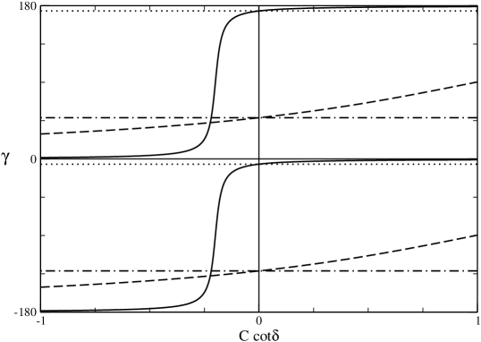
Figure 1: Values “determined” for $\gamma$, as a function of the theoretical input for $C\cot{\delta}$, assuming $\sin{(2\tilde{\beta})}=0.736$, $C=0.0528$, and $S=-0.585$. The solid (dashed) curves correspond to $\gamma_{+}$ ($\gamma_{-}$). The horizontal dotted (dash-dotted) lines correspond to the values of $\gamma$ for which $\tan{\gamma}=L_{+}$ ($\tan{\gamma}=L_{-}$). Here we choose $\cos{(2\tilde{\beta})}$ positive, as in the SM.

Unfortunately, we must contend with the discrete ambiguities. First we notice that, due to the twofold discrete ambiguity in the inversion of the function $\tan{\gamma_{-}}$, $L_{-}$ also produces the bound $\gamma_{-}\geq-132^{\circ}$, for $\gamma_{-}$ in the range $-180^{\circ}\leq\gamma_{-}<0^{\circ}$. We can exclude solutions with negative $\gamma$ if we assume that there is no new physics in the $K-\overline{K}$ system (and trust the sign of the relevant hadronic matrix element).

We must also consider the bound from $L_{+}$. Since both $C\cot{\delta}$ and $I_{+}$ are positive, we obtain $\tan{\gamma_{+}}\geq L_{+}$. This means that $\gamma_{+}\geq 174^{\circ}$, for $\gamma\in(0^{\circ},180^{\circ})$; or $\gamma_{+}\geq-6^{\circ}$, if we take $\gamma\in(-180^{\circ},0^{\circ})$. In both ranges of $\gamma$, the bound from $L_{+}$ is much tighter than the bound from $L_{-}$. We conclude that $\gamma$ is constrained by the bound from $L_{-}$.

We can see from FIG. 1 that our assumption of positive $C\cot{\delta}\geq 0$ plays a crucial role. Indeed, when we cross $C\cot{\delta}=0$ the lower bounds become upper bounds. Moreover, in the region of negative $C\cot{\delta}$, $\gamma_{+}$ goes through a region of vary rapid variation and it even crosses $\gamma_{-}$. This occurs for

$$C\cot{\delta}=-\frac{S+\sin{(2\tilde{\beta})}}{\cos{(2\tilde{\beta})}}=-0.223,$$ (30)

as can be seen in the figure and understood from Eq. (29). The usual assumption that $C\cot{\delta}$ (which is proportional to $\cos{\delta}$) is positive, hinges on the belief that the magnitude of $\delta$ should be small and that the corresponding matrix element should have the sign obtained from factorization. However, it could be that the ratio of “penguin to tree” has a sign opposite to that taken from factorization, in which case $\delta\sim 180^{\circ}$ and $C\cot{\delta}$ would be negative Wolf-sign . We have shown that, if that is the case, this analysis can still be performed, but with the lower bounds becomming upper bounds. Unfortunately in this case $L_{+}$ will provide the effective upper bound $\gamma\leq 174^{\circ}$, which is useless. It is important to stress that, for $\gamma$ negative, the assumption consistent with QCD factorization is $C\cot{\delta}<0$, as is evident from the $\sin{\gamma}$ term in Eq. (16) and from the previous discussion.

The problem of $\gamma_{+}$ crossing $\gamma_{-}$, seen in FIG. 1 for $C\cot{\delta}<0$, will come back to haunt us when we consider the possibility that $\cos{(2\tilde{\beta})}<0$, because of the $\cos{(2\tilde{\beta})}\rightarrow-\cos{(2\tilde{\beta})}$, $\cot{\delta}\rightarrow-\cot{\delta}$, $\tan{\gamma_{\pm}}\rightarrow-\tan{\gamma_{\mp}}$ symmetry we alluded to at the end of section III. This symmetry is clear from the comparizon of FIG. 1 with FIG. 2, drawn for the same $\sin{(2\tilde{\beta})}=0.736$, $C=0.0528$, and $S=-0.585$ “experimental” observables, but assuming the negative $\cos{(2\tilde{\beta})}=-0.677$ possibility.

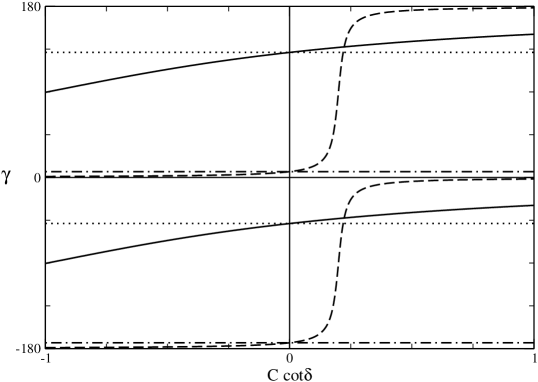
Figure 2: Values “determined” for $\gamma$, as a function of the theoretical input for $C\cot{\delta}$, assuming $\sin{(2\tilde{\beta})}=0.736$, $C=0.0528$, and $S=-0.585$. The solid (dashed) curves correspond to $\gamma_{+}$ ($\gamma_{-}$). The horizontal dotted (dash-dotted) lines correspond to the values of $\gamma$ for which $\tan{\gamma}=L_{+}$ ($\tan{\gamma}=L_{-}$). Here we choose $\cos{(2\tilde{\beta})}$ negative.

For $\cos{(2\tilde{\beta})}=-0.677$, we obtain $I_{+}=0.992$, $L_{+}=-1.12$, $I_{-}=-0.195$ and $L_{-}=0.11$. (This was to be expected from the fact that $\cos{(2\tilde{\beta})}\rightarrow-\cos{(2\tilde{\beta})}$ leads to $L_{\pm}\rightarrow-L_{\mp}$.) If we keep our assumption that $C\cot{\delta}\geq 0$, then $\tan{\gamma_{+}}\geq L_{+}$, meaning that $\gamma_{+}\geq 132^{\circ}$, if we take $\gamma\in(0^{\circ},180^{\circ})$, or $\gamma_{+}\geq-48^{\circ}$, if we take $\gamma\in(-180^{\circ},0^{\circ})$. Again, we may assume the SM in the $K-\overline{K}$ system to exclude the last possibility.

Unfortunately, $L_{-}$ only provides the very poor bound $\arctan{L_{-}}=6^{\circ}$. It is true that this problem can be avoided by ignoring the $\cos{(2\tilde{\beta})}<0$ solution. But, if we are assuming new physics, we should not discard this possibility in an ad-hoc way (as is sometimes done). Amusingly, when $\cos{(2\tilde{\beta})}<0$, it is the assumption that factorization yields the wrong sign for $\delta$ (and, thus, that $C\cot{\delta}<0$) that provides us with bounds on $\gamma$ in the $(0^{\circ},180^{\circ})$ region.

The previous case was motivated by the theoretical expectations $r\,R_{b}=0.11$, $\delta=0.15$, and $\gamma=60^{\circ}$. FIG. 3 shows the same analysis performed for $\sin{(2\tilde{\beta})}=0.736$, $\cos{(2\tilde{\beta})}$ positive, and assuming the current Babar central values $C=-0.19$, and $S=-0.40$ Babar-pipi .

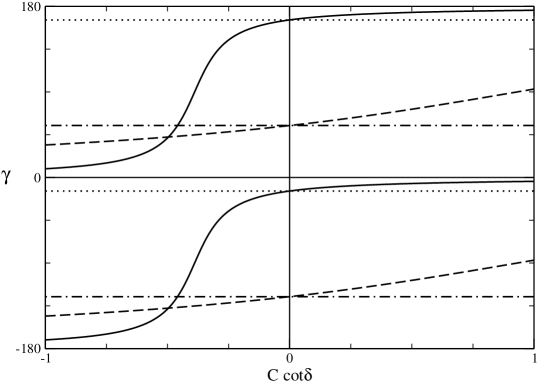
Figure 3: Values “determined” for $\gamma$, as a function of the theoretical input for $C\cot{\delta}$, assuming $\sin{(2\tilde{\beta})}=0.736$, $C=-0.19$, and $S=-0.40$. The solid (dashed) curves correspond to $\gamma_{+}$ ($\gamma_{-}$). The horizontal dotted (dash-dotted) lines correspond to the values of $\gamma$ for which $\tan{\gamma}=L_{+}$ ($\tan{\gamma}=L_{-}$). Here we choose $\cos{(2\tilde{\beta})}$ positive, as in the SM.

The solution with $\cos{(2\tilde{\beta})}$ negative can be obtained through the symmetry already described. We find that $\gamma\geq 55^{\circ}$, if we take $C\cot{\delta}\geq 0$ and $\gamma\in(0^{\circ},180^{\circ})$.

IV.3 Recovering the Buchalla-Safir bound

Buchalla and Safir BS have considered a particular case of the bounds in Eq. (23), which corresponds to setting $C=0$ and assuming the SM. Indeed, they argue that the current (SM) constraints on $\gamma$ eliminate all solutions except the one arising from the canonical inversion of $L_{-}$. Indeed, restricting $\gamma$ to $(0,\pi)$ eliminates four solutions; assuming the SM eliminates the possibility that $\cos{(2\tilde{\beta})}<0$; and the other current bounds on $\gamma$ eliminate $\gamma_{+}$.

Taking $C\cot{\delta}\ (C\cot{\delta}+I_{-})\ I_{-}>0$, we obtain

$$\tan{\gamma_{-}}\geq L_{-}\,.$$ (31)

This would be the simple generalization of the BS bound to the $C\neq 0$ case, if we were to ignore all the discrete ambiguities.

Their (lowest) bound is obtained by setting $C$ to zero in Eq. (26):

$$L_{-}^{0} = \frac{-1-\sqrt{1-S^{2}}\cos{(2\beta)}-S\sin{(2\beta)}}{S\cos{(2\beta)}-\sqrt{1-S^{2}}\sin{(2\beta)}},$$ (32)

$$= \frac{-\cos{(2\beta)}-\sqrt{1-S^{2}}+1+S\sin{(2\beta)}+\cos{(2\beta)}\sqrt{1-S^{2}}}{S-\sin{(2\beta)}-S\cos{(2\beta)}+\sqrt{1-S^{2}}\sin{(2\beta)}},$$ (33)

$$= \frac{\cos{(2\beta)}+\sqrt{1-S^{2}}}{\sin{(2\beta)}-S}.$$ (34)

Eq. (32) results directly from Eq. (26); Eq. (33) is a slightly rewritten version of the expression in BS . They are both equal to the simplest form in Eq. (34). Now,

$$L_{-}-L_{-}^{0}=\frac{(\sqrt{1-S^{2}}-\sqrt{1-C^{2}-S^{2}})(S+\sin{(2\beta)})}{\left[S\cos{(2\beta)}-\sqrt{1-C^{2}-S^{2}}\sin{(2\beta)}\right]\left[S\cos{(2\beta)}-\sqrt{1-S^{2}}\sin{(2\beta)}\right]}.$$ (35)

Since $\sqrt{1-C^{2}-S^{2}}\leq\sqrt{1-S^{2}}$, the numerator is positive whenever $S\geq-\sin{(2\beta)}$. It is true that the denominator will be negative when the two terms between the square brackets have opposite signs. But that only occurs because $\arctan{L_{-}}$ goes through $90^{\circ}$ before $\arctan{L_{-}^{0}}$, and it does not affect the order of the bounds on $\gamma$ explain . As a result, eliminating all the discrete ambiguities, we recover the BS bound

$$\tan{\gamma_{-}}\geq L_{-}^{0},$$ (36)

which is valid for $S\geq-\sin{(2\beta)}$ BS .

FIG. 4 compares the bounds on $\gamma$ obtained from $L_{-}$ as a function of $S$, for different choices of $|C|$ (notice that the value of $L_{-}$ does not depend on the sign of $C$).

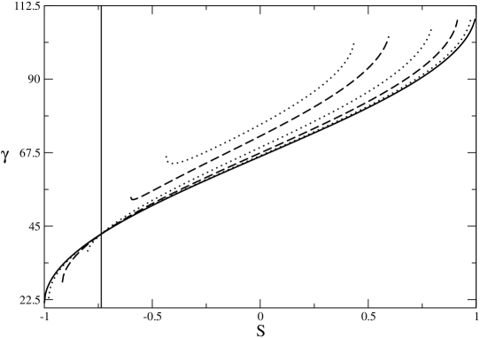
Figure 4: Bounds on $\gamma$ obtained from $L_{-}$ as a function of $S$, for different choices of $|C|$. The vertical line corresponds to $S=-\sin{(2\beta)}$. To the right of it, the solid line (which corresponds to $C=0$) lies below all other lines, in accordance with the BS bound. The other lines correspond to $|C|=0.2$, $|C|=0.4$, $|C|=0.6$, $|C|=0.8$, and $|C|=0.9$, going from the bottom up.

We have taken $\sin{(2\tilde{\beta})}=0.736$ and $\cos{(2\tilde{\beta})}=+0.677$. The vertical line corresponds to $S=-\sin{(2\beta)}$. To the right of it, the solid line (which corresponds to $C=0$) lies below all other lines, in accordance with the BS bound. The dotted line immediately above was obtained with $|C|=0.2$ and the others correspond to $|C|=0.4$, $|C|=0.6$, $|C|=0.8$, and $|C|=0.9$, respectively. FIG. 4 shows that our $L_{-}$ bound improves on the BS bound, and that its impact becomes more relevant for large $|C|$ values.

We can now understand why Buchalla and Safir required the constraint $S\geq-\sin{(2\beta)}$. They did so for two reasons. First, because the BS bound ($C=0$) only lies below the lines with $C\neq 0$ in that case, as seen clearly in FIG. 4. Second because, for $\gamma\in(0^{\circ},180^{\circ})$, $L_{+}$ lies below $L_{-}$ if $S<-\sin{(2\beta)}$. This can be understood from Eq. (29), recalling that the expressions for $L_{\pm}$ are obtained from those of $\tan{\gamma_{\pm}}$ by setting $C\cot{\delta}$ to zero. But this means that there in nothing fundamental about Buchalla and Safir’s restriction that $S\geq-\sin{(2\beta)}$. Indeed, for $S\geq-\sin{(2\beta)}$, the bound from $L_{-}$ with $C=0$ provides the (lowest) lower bound on $\gamma$. But, for $S<-\sin{(2\beta)}$, the bound from $L_{-}$ with $C=0$ is still useful since it provides the (highest) upper bound on $\gamma$.

IV.4 Dependence of the analysis on the theoretical parameter $Q$

In the previous sections we have used $C\cot{\delta}$ as the one piece of theoretical input required to extract $\gamma$ from the $B\rightarrow\pi^{+}\pi^{-}$ decays. This was choosen in order to compare our new constraints based on $L_{\pm}$ (valid for any $C$ and for $\tilde{\beta}\neq\beta$) with that obtained by Buchalla and Safir in the limit $C=0$. However, the quantity $Q=r\cos{\delta}$ is easier to constrain theoretically and also allows the extraction of $\gamma$. Indeed, one can show that Eq. (24) yields

$$\gamma_{\pm}=-\arctan{\left[\frac{1-R_{\pm}}{I_{\pm}}\right]}+\arcsin{\left[\frac{Q\,(R_{\pm}-1)}{\sqrt{I_{\pm}^{2}+(1-R_{\pm})^{2}}}\right]}.$$ (37)

For the “-” sign, the first term reproduces the BS bound, while the second term shows the correction for $Q\neq 0$.

Given a set of experimental values for $\sin{(2\tilde{\beta})}$, $S$, and $C$, the theoretical parameter $Q$ cannot take any value at random. Fortunately, the limits that those experiments place on $Q$ are built into Eq. (37), since the magnitude of the argument of the function $\arcsin{}$ cannot exceed unity. Therefore

$$Q^{2}\leq\frac{I_{\pm}^{2}+(1-R_{\pm})^{2}}{(1-R_{\pm})^{2}}=\frac{2(1-R_{\pm})-C^{2}}{(1-R_{\pm})^{2}}.$$ (38)

FIG. 5 shows the dependence of $\gamma_{\pm}$ on $Q$ for the same “experimental” values used in FIG. 3. Namely, $\sin{(2\tilde{\beta})}=0.736$, $\cos{(2\tilde{\beta})}$ positive, and assuming the current Babar central values $C=-0.19$, and $S=-0.40$ Babar-pipi .

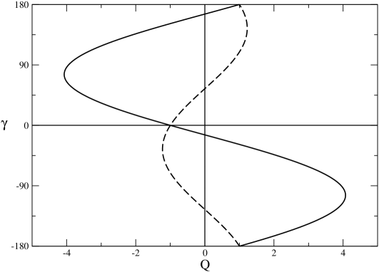
Figure 5: Values “determined” for $\gamma$, as a function of the theoretical input for $Q$, assuming $\sin{(2\tilde{\beta})}=0.736$, $C=-0.19$, and $S=-0.40$. The solid (dashed) curve corresponds to $\gamma_{+}$ ($\gamma_{-}$). Here we choose $\cos{(2\tilde{\beta})}$ positive, as in the SM.

The solution with $\cos{(2\tilde{\beta})}$ negative is easily obtained through the transformations $\gamma_{\pm}\rightarrow-\gamma_{\mp}$, as can be seen directly in Eq. (24). As in FIG. 3, we find that $\gamma\geq 55^{\circ}$, if we take $Q\geq 0$ and $\gamma\in(0^{\circ},180^{\circ})$.

Incidentally, Eq. (38) gives for $|Q|$ the upper bounds of $1.2$ and $4.1$, for the $\gamma_{-}$ and $\gamma_{+}$ branches, respectively, in accordance with FIG. 5.

V Conclusions

The extraction of the CKM angle $\gamma$ from the time-dependent decay $B\rightarrow\pi^{+}\pi^{-}$ requires one piece of external input. Here we have studied the depedence of that analysis on the theoretical parameters $C\cot{\delta}$ or $r\cos{\delta}$. Of course, a similar analysis can be performed with any other input information, such as experimental input from the isospin analysis GL or the SU(3) relation with $B\rightarrow K^{+}\pi^{-}$ SW94 . The novelty introduced by Buchalla and Safir, is that a mild assumption about the theoretical parameters already allows interesting bounds to be placed on $\gamma$ BS .

We have extended their result in several ways: i) we have provided a simpler derivation of their bound, which avoids the Wolfenstein parameters $\rho$ and $\eta$; ii) we have pointed out that the restriction to $S\geq-\sin{(2\tilde{\beta})}$ is not fundamental in the sense that, for $S<-\sin{(2\tilde{\beta})}$, the only change is that the “lowest” bound becomes a “highest” bound; iii) we have highlighted the impact that new physics phases in the $B-\overline{B}$ mixing have, discussing, in particular, the possibility that $\cos{(2\tilde{\beta})}$ might be negative; iv) we have extended their bounds to the case $C\neq 0$. Naturally, the methods applied here can be used in other decays us .

*

Appendix A A useful inequality

Consider the function

$$f(\theta)=A\sin{\theta}+B\cos{\theta}.$$ (39)

Its derivative is zero when

$$\sin{\theta}=\frac{\pm A}{\sqrt{A^{2}+B^{2}}},\ \ \ \ \ \ \ \ \cos{\theta}=\frac{\pm B}{\sqrt{A^{2}+B^{2}}}.$$ (40)

At these points, $f(\theta)$ takes the extremum values $\pm\sqrt{A^{2}+B^{2}}$. Therefore,

$$-\sqrt{A^{2}+B^{2}}\leq A\sin{\theta}+B\cos{\theta}\leq\sqrt{A^{2}+B^{2}}.$$ (41)