Abstract

The theory of the on-shell Sudakov form factor to all orders of logarithms is explained.

1 INTRODUCTION

The key to understanding and using perturbative QCD is the idea of factorization. Factorization is the property that some cross-section or amplitude is a product of two (or more) factors and that each factor depends only on physics happening on one momentum (or distance) scale. The process is supposed to involve some large momentum transfer, on a scale $Q$, and corrections to the factorized form are suppressed by a power of $Q$. (In general the product is in the sense of a matrix product or of a convolution.)

The standard factorization theorems are typified by the one for the moments of the deep inelastic structure functions:

$$F_{n}(Q)=C_{n}\left(\alpha_{\rm s}(Q)\right)\ast\exp\left[\int^{Q}_{Q_{0}}\gamma_{n}\left(\alpha_{s}(\mu)\right)\mathop{{\rm d}\mu}\nolimits/\mu\right]\ast M_{n}(Q_{0}).$$

Here $F_{n}$ is the $n$th moment of one of the structure functions, $C_{n}$ is a Wilson coefficient, $M_{n}$ is a hadronic matrix element of an operator of spin $n$ and twist 2, $\gamma_{n}$ is an anomalous dimension, and $Q_{0}$ is a fixed scale. The symbol ‘$\ast$’ denotes a matrix product (to allow the possibility of contributions from more than one operator). The renormalization group has been used to absorb all logarithms of large mass ratios into the integral over the anomalous dimension. These theorems are described elsewhere in this volume.

In this article, I will treat the Sudakov form factor, which provides the simplest example of factorization theorems of a more complicated kind. The difference between this case and deep inelastic scattering results from a difference in the regions of loop-momentum space that give the leading-twist contributions to the process. In the case of simple factorization theorems like (1), these regions involve lines with momenta that are either collinear to the detected particles or are far off-shell. In individual graphs there are leading twist contributions from regions with soft gluons; but after an intricate cancellation ${}^{\ref{1},\ref{2}]}$, the effects of soft gluons cancel. However, in the Sudakov form factor the effects of the soft gluons do not cancel. Even so, a more general factorization theorem holds for this case.

This form factor is the elastic form factor of an elementary particle in an abelian gauge theory at large momentum transfer $Q$. Sudakov ${}^{\ref{3}]}$ treated the off-shell form factor in the leading logarithmic approximation. I will treat the on-shell case and derive the full factorization formula, which is valid to all orders of perturbation theory and includes all nonleading logarithms.

This relatively simple case is a prototype for such processes as the Drell-Yan cross section when the transverse momentum is much less than the invariant mass of the Drell-Yan pair. A treatment to all orders of logarithms is given in ${}^{\ref{4},\ref{5}]}$, and applications to phenomenology can be found in ${}^{\ref{6},\ref{7}]}$. Work at the leading logarithm level can be found in ${}^{\ref{8},\ref{9}]}$ and references therein. In ${}^{\ref{10}]}$ Sen showed how to treat the on-shell Sudakov form factor in a non-abelian theory to all orders of logarithms.

The first step in proving any factorization theorem is to understand the regions of the space of loop momenta that give the “leading-twist” contributions, i.e. contributions not suppressed by a power of $Q$. After appropriate approximations it is possible to use Ward identities to convert the leading-twist contributions into a form that corresponds to the factorization theorem. A complication here is to eliminate double counting. Finally a differential equation for the evolution of the form factor is derived. It is only after this step that it is possible to perform systematic perturbative calculations, without having the validity of a finite-order calculation being brought into doubt by the possibility of large logarithmic corrections in higher order. The solution to the equation is in terms of quantities with perturbation expansions that have no large logarithmic terms in their coefficients.

One topic I will emphasize is the extent to which the fact that we are dealing with a renormalizable gauge theory of physics comes into the form of the factorization. To do this I will start by examining what sort of result holds in a superrenormalizable theory without gauge fields, specifically $\phi^{3}$ theory in four space-time dimensions. The $\left(\phi^{3}\right)_{4}$ theory is of course completely unphysical. However, it is a simple model which exhibits the features common to any superrenormalizable theory without gauge fields but which has no irrelevant complications. We will see that a very simple factorization holds true.

Next, I will step up the space-time dimension to $d=6$. This will render the model merely renormalizable instead of superrenormalizable. The short-distance part of the factorization will then become non-trivial, but it will still be of the same form as for deep inelastic scattering, (1).

Finally, I will return to four dimensions, but now with a gauge theory. To provide a simple demonstration of how and why all the logarithms are under control, I must avoid complications that are irrelevant for this purpose. So I will take the theory to be abelian, with a massive gluon, and treat the annihilation of a $q\bar{q}$ pair into a virtual photon. The complications thereby avoided include: a non-abelian gauge group, the infra-red divergences caused by a massless gluon (which would mean we would have to discuss a kinematically more complicated process), and color confinement (which would force us to treat, say, a form factor of a composite particle). Although these complications are important for real strong interactions, they are inessential if we are trying to understand “Sudakov” effects by themselves.

2 REDUCED GRAPHS

Consider a form factor

$$F=\langle 0|j(0)|p_{A}p_{B}\rangle.$$

Here $j$ is a composite field, for example the electromagnetic current of quarks in QCD, and $|p_{A}p_{B}\rangle$ represents an incoming two-particle state with energy $Q$:

$$Q^{2}=\left(p_{A}+p_{B}\right)^{2},$$

which we assume to be very large.

First we must find the regions of momentum space that are important in Feynman graphs for this amplitude. We use the method given by Libby and Sterman ${}^{\ref{11}]}$. Suppose we scale all momenta by a factor $Q$:

 

$${k^{\mu}}$$

 

The reduced mass $\tilde{m}$ goes to zero as $Q$ goes to infinity, so that we are effectively going to a massless theory. If all scaled momenta in a graph are off-shell by order unity, then we get a contribution of order unity (given that we are in a renormalizable theory, so that the coupling is dimensionless). Then simple perturbation theory is applicable provided only that the effective coupling $\alpha_{\rm s}(Q)$ is small. Other leading contributions can come from regions where some of the scaled momenta become on-shell in the massless theory $(\tilde{m}=0)$. In this case we obtain a contribution only when the contour of integration is trapped at the on-shell point, for otherwise we may deform the contours into the off-shell region. Such points were called pinch-singular points in ${}^{\ref{11}]}$.

The analysis of Coleman and Norton ${}^{\ref{12}]}$ can be used to locate the pinch singular points. Each pinch-singular point can be represented by a reduced graph. The lines whose scaled momenta are off-shell by order unity are all contracted to points; they form the vertices of the reduced graph for a pinch singular point. The lines that have on-shell scaled momenta form the lines of the reduced graph. In order that the contours of integration be pinched, the reduced graph must represent a classical scattering process. In the case of an annihilation form factor, the reduced graphs have the form exemplified by Fig. 1. The on-shell lines either have non-zero fractions of the scaled momentum of one or other of the incoming lines or they have zero scaled momentum. These lines are represented by solid and dashed lines (respectively), and are called jet and soft lines. An arbitrary number of jet lines parallel to $\tilde{p}^{\mu}_{A}$ interact and enter the reduced vertex where the annihilation occurs. A similar situation occurs for $\tilde{p}_{B}$. An arbitrary number of soft lines join the two jet subgraphs.

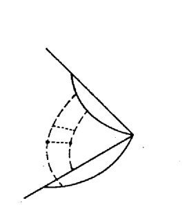
Figure 1: Typical reduced graph for annihilation form factor. Jet lines are solid, and soft lines are dashed.

This can all be said without knowing the field theory. We next need to know which of the pinch singular points give important contributions as $Q\to\infty$. For this purpose we consider only leading twist contributions, i.e., those that are not suppressed by a power of $Q$. Which regions give leading-twist contributions will depend on the theory within which we work, especially on its renormalizability or superrenormalizability and on the presence or absence of gauge particles.

3 SUPERRENORMALIZABLE SCALAR THEORY: $\left(\phi^{3}\right)_{4}$

The Lagrangian of $\phi^{3}$ theory is

$${\cal L}={1\over 2}\left(\partial\phi\right)^{2}-{1\over 2}m^{2}_{B}\phi^{2}-{1\over 6}g\phi^{3}.$$

In $d=4$ space-time dimensions the coupling, $g$, has positive mass dimension. This signals that no infinite coupling or wave function renormalization is needed, i.e., that the theory is superrenormalizable. We define the form factor in eq. (2) by choosing the composite field $j$ to be ${1\over 2}\phi^{2}$.

Figure 2: One loop graphs for form factor in $\phi^{3}$ theory.

First consider the one-loop graphs, which are listed in Fig. 2. The graphs with self-energy corrections, Fig. 2(a) and (b), have reduced graphs equal to themselves. If these and higher-order self-energy graphs were all that we have, then the form factor would be equal to

$$z(m^{2},g),$$

where $z$ is the residue of the renormalized propagator:

$$S_{F}(p^{2},m^{2},g)\to{iz\over p^{2}-m^{2}}\quad\hbox{as $p^{2}\to m^{2}$}.$$

In fact these graphs are all that we have, for vertex graphs like Fig. 2(c) vanish as $Q\to\infty$, by a power $Q$, as we will now show. Fig. 2(c) has the value

$$\openup 6.45831pt\halign to=0.0pt{\hfil$\displaystyle{#}$ &$\displaystyle{{}#}$\hfil&\llap{$#$}\cr\Gamma_{c}&={-ig^{2}\over(2\pi)^{4}}\int\mathop{{\rm d}^{4}k}\nolimits {1\over(m^{2}-k^{2}) \left[m^{2} - (p_{A}+k)^{2} \right] \left[m^{2} - (p_{B}-k)^{2} \right]} &\hbox to0.0pt{\hss$(8)\cr&={-ig^{2}\over(2\pi)^{4}Q^{2}} \int\mathop{{\rm d}^{4}\tilde{k}}\nolimits {1\over(\tilde{m}^{2} - \tilde{k}^{2}) \left[ \tilde{m}^{2} - (\tilde{p}_{A} + \tilde{k})^{2} \right] \left[\tilde{m}^{2} - (\tilde{p}_{B} - \tilde{k})^{2} \right]} \cr&&\hbox to0.0pt{\hss$(9)\crcr}}}$$

The possible reduced graphs for Fig. 2(c) are listed in Fig. 3:

1. Fig. 3(a) corresponds to the region that $|\tilde{k}^{\mu}|\sim 1$, i.e. where all internal lines are far off-shell. Manifestly the resulting contribution is $O\left(1/Q^{2}\right)$. This is essentially a result of dimensional analysis coupled with the positive dimension of $g$.

2. Fig. 3(b) corresponds to the region where $k^{\mu}$ is collinear to $p_{A}^{\mu}$. This graph is also $O\left(1/Q^{2}\right)$. To see this, we use light cone coordinates

   $$p^{-}_{B}=p^{+}_{A}={Q\over\sqrt{2}},\qquad p^{+}_{B}=p^{-}_{A}={m^{2}\over Q\sqrt{2}}.$$

   Then in the region symbolized by Fig. 3(b), we have

   $$k^{+}=O(Q),\quad k^{-}=O(\lambda^{2}Q),\quad k_{T}=O(\lambda Q),$$

   where $\lambda$ is small. It is now easy to check that the contribution to the form factor is $O\left(1/Q^{2}\right)$. The point is that one quark line is far off-shell and that there are no compensating numerator factors.

3. Fig. 3(c) is just Fig. 3(b) with $A\leftrightarrow B$.

4. For Fig. 3(d), which corresponds to the region where all components of $k^{\mu}$ are much less than $Q$, we let

   $$k^{\mu}=O\left(\lambda Q\right),$$

   for all components. Again we get a contribution of order $1/Q^{2}$.

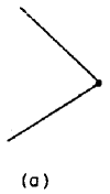
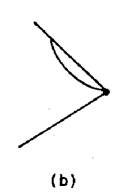
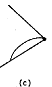
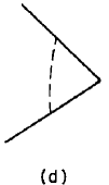
Figure 3: Reduced graphs for Fig. 2(c).

It is fairly easy to show that this analysis holds true to all orders, by the methods of ${}^{\ref{11}]}$. The reduced graphs for the leading twist contributions all have the form of self energy graphs attached to the lowest order vertex, so that the form factor is $z$ plus higher-twist contributions. (See eq. (7) for the definition of $z$.)

4 RENORMALIZABLE SCALAR THEORY: $(\phi^{3})_{6}$

4.1 One-loop

The sole significant difference in going to six space-time dimensions is caused by the coupling’s becoming dimensionless and the consequent need for coupling and wave function renormalization. We write the Lagrangian in the form:

 

$${{\cal L}={}}$$

 

Here $m$ and $g$ are the renormalized mass and coupling, and the last four terms are the renormalization counterterms. We will use dimensional regularization (i.e., space-time dimension $d=6-2\epsilon$) to cut off the ultra-violet divergences. To keep the coupling $g$ dimensionless we introduce the unit of mass ${}^{\ref{13}]}$ $\mu$. The linear term $h\phi$ is adjusted to cancel tadpole graphs; for the other terms we will use $\overline{{\rm MS}}$ renormalization ${}^{\ref{14}]}$.

The structure of the reduced graphs is the same, as always. What changes is the size of the contributions. Consider the one-loop vertex graph Fig. 2(c), whose reduced graphs are in Fig. 3. By following the same method as we used in Sec. 3, we find that the contributions of the reduced graphs (at $d=6$) are

 

Fig. 3(a) $${{}Q^{0},}$$

Fig. 3(b) or (c)

Fig. 3(d)

 

Clearly we get a leading contributions solely from the region where all internal lines are far off-shell. The existence of this contribution is tied to the dimensionlessness of the coupling.

The contribution of Fig. 2(c) is therefore given by neglecting all masses, with errors of order $1/Q^{2}$. Thus

$$\Gamma_{c}\sim-{ig^{2}\over(2\pi)^{6}}(2\pi\mu)^{2\epsilon}\int\mathop{{\rm d}^{6-2\epsilon}k}\nolimits{1\over(-k^{2})\left[-(\hat{p}_{A}+k)^{2}\right]\left[-(\hat{p}_{B}-k)^{2}\right]}+{}\hbox{counterterm}.$$

Here $\hat{p}_{A}^{\mu}$ and $\hat{p}^{\mu}_{B}$ are light-like vectors close to $p_{A}^{\mu}$ and $p_{B}^{\mu}$:

 

$${(\hat{p}^{+}_{A},\hat{p}^{-}_{A})}$$

 

After using $\overline{{\rm MS}}$ renormalization to cancel the ultraviolet divergence in the integral in (14), we find

$$\Gamma_{c}={g^{2}\over 128\pi^{3}}\left[-\ln(-Q^{2}/\mu^{2})+3\right]+O(1/Q^{2}).$$

(At one-loop order, the $\overline{{\rm MS}}$ scheme is defined by requiring counterterms to be a coefficient times $1/\epsilon-\gamma+\ln(4\pi)$, where $\gamma$ is Euler’s constant. In the MS scheme we would omit the $\gamma$ and the $\ln(4\pi)$.)

4.2 Higher orders

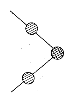
Figure 4: General graph for form factor. The cross-hatched bubble is the sum of all 1PI graphs for the form factor.

The generalization to all orders of the one-loop results is obtained by observing that the graphs for the form factor are a product of two propagators and a one-particle-irreducible (1PI) vertex (Fig. 4). A leading contribution is only obtained from the 1PI vertex when all its internal lines are off-shell by order $Q^{2}$. It can be shown fairly easily that other regions are power suppressed ${}^{\ref{15}]}$. Thus the only leading reduced graphs have the form of Fig. 5. This result is true in any renormalizable non-gauge theory.

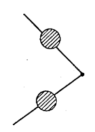
Figure 5: Leading reduced graphs for form factor in $(\phi^{3})_{6}$ theory.

Therefore the form factor has the form

$$F=z(g,m/\mu)\,\Gamma(Q/\mu,g)+O\left((\hbox{logarithms of $Q$})/Q^{2}\right).$$

Here $\Gamma$ is the 1PI vertex with the masses set to zero. This is the simplest example of a factorization theorem. The $z$ factor comes from the single-particle propagator; it depends on phenomena on the scale of the quark mass $m$ and is independent of the energy $Q$. On the other hand the vertex factor $\Gamma$ depends only on the total energy and not on the mass.

Since the theory needs renormalization, there is important dependence on the unit of mass $\mu$. A perturbative calculation of $z$ or $\Gamma$ has large logarithms of $m/\mu$ or of $Q/\mu$, so a simultaneous direct calculation of these quantities to low order cannot be reliable if $Q/m$ is large enough. The renormalization group comes to our aid since both $z$ and $\Gamma$ satisfy renormalization group equations ${}^{\ref{16},\ref{17}]}$

$$\openup 6.45831pt\halign to=0.0pt{\hfil$\displaystyle{#}$ &$\displaystyle{{}#}$\hfil&\llap{$#$}\cr\mu{\mathop{{\rm d}}\nolimits\over\mathop{{\rm d}\mu}\nolimits} z&=-2\gamma\left(g\left(\mu\right)\right) &\hbox to0.0pt{\hss$(18)\cr\mu{ \mathop{{\rm d}}\nolimits \over\mathop{{\rm d}\mu}\nolimits} \Gamma&=-\gamma_{\phi^{2}} \left(g\left(\mu\right)\right)+2\gamma\left(g\left(\mu\right)\right) \cr&\equiv-\hat{\gamma}\left(g\left(\mu\right)\right). &\hbox to0.0pt{\hss$(19)\cr}}}$$

Here $\gamma(g)$ and $\gamma_{\phi^{2}}(g)$ are the anomalous dimensions of the operators $\phi$ and $\phi^{2}$ respectively, and the renormalization-group operator is

$$\mu{\mathop{{\rm d}}\nolimits\over\mathop{{\rm d}\mu}\nolimits}\equiv\mu{\partial\over\partial\mu}+\beta(g){\partial\over\partial g}+\gamma_{\phi^{2}}\,m^{2}{\partial\over\partial m^{2}}.$$

Note that $\gamma$ is half its value as defined by many authors.

Evidently we can solve Eqs. (18) and (19) and write

 

$${F(Q,m,g,\mu)={}}$$

 

Here $g(\mu)$ is the running (or effective) coupling at scale $\mu$. Evidently each factor may be reliably calculated without large logarithms in higher-order corrections.

4.3 “Optimization” of perturbation calculations

In (21) the endpoints of the integrals over $\mu^{\prime}$ are $\mu^{\prime}=m$ and $\mu^{\prime}=Q$. This is not necessary; all that is needed is that the endpoints be of order $m$ and $Q$. This is important in “optimizing” perturbative calculations. We can write

 

$${F(Q,m,g,\mu)=z\left(g(c_{1}m),1/c_{1}\right)}$$

 

Here $c_{1}$ and $c_{2}$ are arbitrary constants to be chosen at will. In a calculation to all orders of perturbation theory the result for $F$ is independent of our choice of $c_{1}$ and $c_{2}$. But in a finite order calculation the result has dependence on $c_{1}$ and $c_{2}$ of the order of the first uncalculated term. We should choose $c_{1}$ and $c_{2}$ not too far from unity to keep higher order corrections small. The change in $\Gamma$ given by varying $c_{1}$ and $c_{2}$ by a factor of 2 can be regarded as an estimate of the error in the calculation induced by uncalculated higher order terms.

There has been much discussion ${}^{\ref{18}]}$ of appropriate ways to choose $c_{1}$ and $c_{2}$.

5 GAUGE THEORIES

We now consider a form factor in the massive abelian gauge theory whose Lagrangian is

 

$${{\cal L}={}}$$

 

Here the notation is standard. The renormalized masses and coupling are $m$, $M$ and $g$. We regulate ultra-violet divergences by continuing to space-time dimension $d=4-2\epsilon$, and we will call $A_{\mu}$ the gluon field and $q$ the quark field. We will treat the electromagnetic form factor of the quark

$$F=\left<0\left|\,[\bar{q}\gamma^{\mu}q](0)\,\right|q(p_{A}),\bar{q}(p_{B})\right>,$$

when the center-of-mass energy $Q$ $\left(\equiv\sqrt{(p_{A}+p_{B})^{2}}\right)$ gets large compared to all masses.

Sudakov ${}^{\ref{3}]}$ was the first to discuss such a form factor to all orders of perturbation theory. His result was for the sum of all the leading logarithms, but with the quarks off-shell and a massless photon. He found that $F\sim\exp\left[-(g^{2}/8\pi^{2})\ln^{2}(Q^{2})\right]$. The on-shell case, with a massive photon, was first treated (still in leading logarithm approximation) by Jackiw ${}^{\ref{19}]}$, with the result that $F\sim\exp\left[-(g^{2}/16\pi^{2})\ln^{2}(Q^{2})\right]$.

From Sudakov’s work (1956) until 1980, there was no progress in going systematically beyond leading logarithms, despite many attempts. Mueller ${}^{\ref{20}]}$ and Collins ${}^{\ref{21}]}$ then gave an all-orders and all-logarithms treatment. The treatment below is an improved version of ${}^{\ref{21}]}$. A first version of the present treatment appeared ${}^{\ref{22}]}$ as notes on lectures given in 1984.

Notice that in these gauge theory form factors there are two logarithms of $Q$ per loop rather than the one logarithm per loop that we have in $(\phi^{3})_{6}$ theory. This is a symptom of the new physics present in a gauge theory. The effects that we will investigate reappear in many processes in QCD.

5.1 One loop

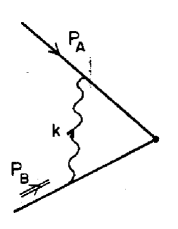
Figure 6: One loop vertex in QED.

Self-energy graphs contribute just as they do in $\phi^{3}$ theory, and give an overall factor $z_{2}(g,m,M,\mu)$, the residue of the pole of the quark propagator. So the only non-trivial one-loop graph is the vertex graph, Fig. 6. Its value is

 

$${{ig^{2}\over 16\pi^{4}}}$$

 

where the numerator of the gluon propagator is

$$N_{\lambda\nu}(k)=g_{\lambda\nu}-k_{\lambda}k_{\nu}(1-\xi)/\left(k^{2}-\xi m^{2}+i\epsilon\right).$$

The possible reduced graphs are exactly the same as in $\phi^{3}$ theory and are listed in Fig. 3.

Since our theory has a dimensionless coupling, the ultraviolet region, of large $k$, contributes to the leading power of $Q$, just as in $\phi^{3}$ theory in six dimensions. However, unlike $\phi^{3}$ theory in either dimension, the other three regions also give leading contributions. This happens because the numerator factor in (25) is $O(Q^{2})$ in all three regions; we know from our analysis of $\phi^{3}$ theory that the graph would otherwise be of order $1/Q^{2}$. We must first understand exactly how this factor of $Q^{2}$ arises, since a systematic treatment of such enhancements by numerators is the key to a complete treatment of the form factor to all orders of perturbation theory. The mere fact that the reduced graphs Fig. 3(b), (c) and (d) are leading twist means that a simple factorization like (17) or (21) cannot hold.

5.2 Method of Grammer and Yennie

Consider the region corresponding to the reduced graph of Fig. 3(b). This is where $k^{\mu}$ is collinear to $p^{\mu}_{A}$ — see eq. (11). In this region the gluon is moving slowly relative to the quark, $p^{\mu}_{A}$, and we may regard the gluon and the virtual quark $p_{A}+k$ as being given a large boost from the center-of-mass frame. Thus the term in

$$({\hbox{$p$}\kern-2.51563pt\kern-2.5pt\hbox{$/$}\kern 2.51563pt\kern-2.5pt}_{A}+{\hbox{$k$}\kern-2.76042pt\kern-2.5pt\hbox{$/$}\kern 2.76042pt\kern-2.5pt}+M)\gamma^{\lambda}u(p_{A}),$$

with $\lambda=+$ is by far the largest.

It follows that the sum over $\nu$ in (25) is dominated by the term with $\nu=-$. (Remember that in light-cone coordinates the metric is non-diagonal: $g_{+-}=g_{-+}=1$, $g_{++}=g_{--}=0$.)

Note that we cannot say that the sum over $\lambda$ is dominated by $\lambda=+$, because of the $k_{\lambda}k_{\nu}$ terms in the gluon propagator. (Even if we set $\xi=1$, so that we used Feynman gauge, such terms would arise when we consider graphs with vacuum polarization corrections for the gluon).

A more general argument giving the same answer can be made by treating all the $\gamma$-matrices as order 1. We wish to see how the numerator terms with large components, viz. $p^{+}_{A}$, $k^{+}$, $p^{-}_{B}$ contribute. To do this, we anticommute all $\gamma^{-}$’s to the left and all $\gamma^{+}$’s to the right and use ${\gamma^{+}}^{2}={\gamma^{-}}^{2}=0$. Then we use the mass-shell conditions

 

$${({\hbox{$p$}\kern-2.51563pt\kern-2.5pt\hbox{$/$}\kern 2.51563pt\kern-2.5pt}_{A}-M)u(p_{A})}$$

 

Since $k^{+}$ and $p^{+}_{A}$ always multiply a $\gamma^{-}$ in the numerator and since $p^{-}_{B}$ always multiplies a $\gamma^{+}$, we find that the large terms only arise from anticommuting a $\gamma^{-}$ with the $\gamma^{\lambda}$ or a $\gamma^{+}$ with the $\gamma^{\nu}$.

Let us write the numerator as

$$\gamma^{\nu}(-{\hbox{$p$}\kern-2.51563pt\kern-2.5pt\hbox{$/$}\kern 2.51563pt\kern-2.5pt}_{B}+{\hbox{$k$}\kern-2.76042pt\kern-2.5pt\hbox{$/$}\kern 2.76042pt\kern-2.5pt}+M)\gamma^{\mu}({\hbox{$p$}\kern-2.51563pt\kern-2.5pt\hbox{$/$}\kern 2.51563pt\kern-2.5pt}_{A}+{\hbox{$k$}\kern-2.76042pt\kern-2.5pt\hbox{$/$}\kern 2.76042pt\kern-2.5pt}+m)\gamma^{\lambda}N_{\lambda\nu}=B^{\nu}\gamma^{\mu}A_{\nu},$$

with $B^{\nu}=\gamma^{\nu}(-{\hbox{$p$}\kern-2.51563pt\kern-2.5pt\hbox{$/$}\kern 2.51563pt\kern-2.5pt}_{B}+{\hbox{$k$}\kern-2.76042pt\kern-2.5pt\hbox{$/$}\kern 2.76042pt\kern-2.5pt}+M)$. To simplify this, we use a beautiful trick formalized by Grammer and Yennie ${}^{\ref{24}]}$. It starts by making the following string of approximations

 

$${B^{\nu}A_{\nu}}$$

 

Here we rely on the facts that $+$ components of $A^{\nu}$ and $k^{\nu}$ are their largest and that the $-$ component of $B^{\nu}$ is not much smaller than its other components. To put the result in covariant form, we have defined $u^{\mu}_{B}$ to be a light-like vector with $u^{-}_{B}=1$, $u^{+}_{B}=u^{T}_{B}=0$.

We now have a factor $k_{\nu}$ times the lower vertex. This is a standard situation where Ward identities can be used. In the present case the result is easy to derive:

 

$${\bar{v}(p_{B})k_{\nu}B^{\nu}}$$

 

where we used the on-shell condition (27) for the wave function. The factor $(p_{B}-k)^{2}-M^{2}$ cancels the antiquark propagator and we find that if $k^{\mu}$ is restricted to be collinear to $p^{\mu}_{A}$, then

$$\Gamma\simeq{-ig^{2}\over 16\pi^{4}}\ \int_{{\scriptstyle k\ {\rm collinear}\atop\scriptstyle{\rm to\ }p_{A}}}\ \mathop{{\rm d}^{4}k}\nolimits{\bar{v}(p_{B})u^{\nu}_{B}\gamma^{\mu}({\hbox{$p$}\kern-2.51563pt\kern-2.5pt\hbox{$/$}\kern 2.51563pt\kern-2.5pt}_{A}+{\hbox{$k$}\kern-2.76042pt\kern-2.5pt\hbox{$/$}\kern 2.76042pt\kern-2.5pt}+M)\gamma^{\lambda}u(p_{A})\over k\cdot u_{B}\left(m^{2}-k^{2}\right)\left[M^{2}-\left(p_{A}+k\right)^{2}\right]}N_{\lambda\nu}(k),$$

with errors being smaller by a power of $1/Q$ (or $\lambda$, where $\lambda$ is the small scale factor in eq. (11)).

The coupling of the gluon to the antiquark has become featureless; it is in fact insensitive to the spin and energy of the antiquark. All the gluon sees is the direction and charge of the antiquark. We do not need an $i\epsilon$ prescription for the pole of $1/k\cdot u_{B}$ at $k^{+}=0$, for $k^{+}$ is always large in the collinear region.

An exactly similar result holds for the opposite collinear region (Fig. 3(c))

$$\Gamma\sim{-ig^{2}\over 16\pi^{4}}\int_{{\scriptstyle k\ {\rm collinear}\atop\scriptstyle{\rm to\ }p_{B}}}\ \mathop{{\rm d}^{4}k}\nolimits{\bar{v}(p_{B})\,\gamma^{\nu}(-{\hbox{$p$}\kern-2.51563pt\kern-2.5pt\hbox{$/$}\kern 2.51563pt\kern-2.5pt}_{B}+{\hbox{$k$}\kern-2.76042pt\kern-2.5pt\hbox{$/$}\kern 2.76042pt\kern-2.5pt}+M)\gamma^{\mu}u^{\lambda}_{A}u(p_{A})\over[M^{2}-(p_{B}-k)^{2}](m^{2}-k^{2}-i\epsilon)(u_{A}\cdot k)}N_{\lambda\nu}(k).$$

Furthermore a slightly different result holds if $k^{\mu}$ is in the soft region, symbolized by the reduced graph Fig. 3(d):

$$\Gamma\sim{ig^{2}\over 16\pi^{4}}\int_{\rm soft}\mathop{{\rm d}^{4}k}\nolimits{\bar{v}(p_{B})u^{\nu}_{B}\gamma^{\mu}u^{\lambda}_{A}u(p_{A})N_{\lambda\nu}(k)\over\left(u_{B}\cdot k-i\epsilon\right)\left(m^{2}-k^{2}-i\epsilon\right)\left(u_{A}\cdot k+i\epsilon\right)}.$$

The only subtlety in the derivation of this equation is that we must assume that all components of $k$ are comparable (or at least that $|k^{+}/k^{-}|$, $|k^{-}/k^{+}|\ll Q^{2}/M^{2}$, $|k^{+}k^{-}|\mathrel{\;{\hbox{\raise 1.50696pt\hbox{$>$}}\kern-3.8889pt\kern-3.8889pt\hbox{\lower 2.79857pt\hbox{$\sim$}}}\;}k^{2}_{T}$). However, there is a leading contribution when $k^{+}$ and $k^{-}$ are of order $\lambda^{2}Q$ and $k_{T}$ is of order $\lambda Q$, with $\lambda$ a small quantity. This is the Glauber region ${}^{\ref{25}]}$, and there none of the approximations (31) to (33) is valid. Now, in the Glauber region $m^{2}-k^{2}\sim m^{2}+k^{2}_{T}$, independently of $k^{+}$ and $k^{-}$. So we can get out of this region by deforming the contours of integration over $k^{+}$ and $k^{-}$ away from the poles in the quark and antiquark propagators to where at least one of (31) to (33) is valid. To indicate the direction of deformation, we introduced the $i\epsilon$’s with the $u_{A}\cdot k$ and $u_{B}\cdot k$ denominators.

Note that there are overlap regions for $k$ where two or more of the approximations (31) to (33) are simultaneously valid. We will see shortly how to avoid the double counting that this could give in the factorization theorem.

The physics of the general case is visible from the one-loop case. The simplification in going from eq. (25) to any of (31) to (33) is to replace one or both quark lines by an eikonal approximation. That is, the quark is replaced by a source of the appropriate charge that exists along a light-like line in either the $+$ or $-$ direction, and recoil of the approximated quark is neglected. What is happening is that there is a large relative rapidity between the gluon and the approximated quark. The gluon only sees a Lorentz-contracted object of a certain charge moving at the speed of light in a certain direction. On the other hand the quark only sees the gluon for only a short time in the quark’s rest frame immediately before the annihilation.

5.3 Leading regions for general graph

The manipulations in the preceding sections have succeeded in simplifying the integrand of (25) in the regions where $k^{\mu}$ remains close to mass-shell as $Q$ goes to infinity. We will use these results, and their generalization to higher order to construct a useful factorized form for the complete form factor.

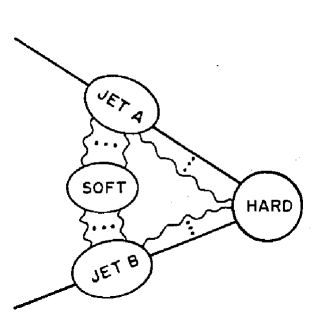
Figure 7: Leading regions for quark form factor.

The first step (in the general case) is to see that, for a general graph $\Gamma$, all the regions that give leading-twist contributions have ${}^{\ref{11}]}$ the form of Fig. 7. Each region is specified by dividing the graph into four subgraphs, designated “jet-A”, “jet-B”, “soft”, and “hard”. In the subgraphs jet-A and jet-B, the momenta of the internal lines satisfy $|k^{+}|\gg|k^{-}|$ and $|k^{-}|\gg|k^{+}|$ respectively. A quark line from jet-A and an antiquark from jet-B enter the hard subgraph, together with arbitrarily many gluons. The hard subgraph also includes the vertex for the current. The momenta of the internal lines of the hard subgraph satisfy $|k^{2}|\gg M^{2}$. The soft subgraph consists of lines all of whose momentum components are much less than $Q$. The external lines of the soft subgraph are all gluons and attach to one or other of the jet subgraphs. Some regions have no soft subgraph.

Each of the jet subgraphs and the hard subgraph is connected. The soft subgraph, if present, may consist of more than one connected component; but each of its components must be joined to both jet-A and jet-B.

Note that within the jet and soft subgraphs there may be loops with large ultra-violet momenta. These make up vertices of the reduced graphs (as in Fig. 1). These reduced vertices are of the same form as the ordinary vertices of the theory if the corresponding regions of momentum space are to give leading twist contributions.

We must be more precise about the regions represented by Fig. 7. The momenta satisfy the following requirements. The value of $|k^{+}/k^{-}|$ for the momentum of a soft line must be much less than the value of this ratio for the lines in the jet-$A$ subgraph and must be much greater than the ratio for the lines in the jet-$B$ subgraph. This ensures that the Grammer-Yennie approximation is applicable to the coupling of the soft lines to the collinear lines. The momenta in the hard subgraph must have virtualities that are much greater than for the momenta in the soft and collinear subgraphs. This ensures that the Grammer-Yennie approximation applies to the coupling of collinear gluons to the hard part.

The next step in the proof is to use the same approximations of the Grammer-Yennie type that we used for the one-loop graph. After use of Ward identities, this will give a factorization. Then we will write the factors in terms of matrix elements of certain operators. In general, a given part of the space of loop momenta may be in the intersection of several different regions of the form of Fig. 7. We will have to make an arbitrary choice of which region to use. The resulting factorization will involve graphs with momenta restricted to certain regions of momentum space. We will convert this intermediate factorization to a more useful factorization by showing that operator formulae representing the second factorization can be converted to the same intermediate factorization.

The resulting factorization will still not be in a form that allows perturbative calculations without large logarithms. But it will enable us to derive a differential equation for the $Q$-dependence of the form factor. The solution of this equation will be our ultimate result, and will have all the logarithms separated out.

5.4 Factorization

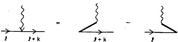
Figure 8: Grammer-Yennie approximation and elementary Ward identity.

When a gluon collinear to $A$ attaches to the hard subgraph, we use approximation (29) where now $B^{\nu}$ denotes the elementary vertex where the collinear gluon attaches to the hard subgraph. We then use a Ward identity of the sort illustrated in Fig. 8. We let the vertex be $B^{\nu}=ig\gamma^{\nu}$ and the momenta of the quarks be $l$ and $l+k$. Then

 

$${{u^{\nu}_{B}k_{\nu^{\prime}}\over k\cdot u_{B}}}$$

 

On the right of Fig. 8 we use the double line to denote the eikonal propagator $i/k\cdot u_{B}$. When we sum over all ways of attaching the jet gluons to the hard subgraph, there is a whole set of cancellations and the effect is to take the gluons to the $A$ side of the hard subgraph, as depicted in Fig. 9. In obtaining this we have used eq. (34) repeatedly. Each gluon has a factor $i/k\cdot u_{B}$. Then, we use identities like

$$\left[{i\over k_{1}\cdot u_{B}}\right]\left[{i\over k_{2}\cdot u_{B}}\right]=\left[{i\over(k_{1}+k_{2})\cdot u_{B}}\right]\left[{i\over k_{1}\cdot u_{B}}\right]\,+\,\left[{i\over(k_{1}+k_{2})\cdot u_{B}}\right]\left[{i\over k_{2}\cdot u_{B}}\right]$$

to write the gluon attachments as if they are to a single line with an eikonal propagator. Physically, Fig. 9 is telling us that the gluons collinear to $A$ only see the charge and direction of the antiquark.

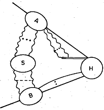
Figure 9: Result of applying Ward identities to attachments of gluons from jet $A$ to the ultraviolet subgraph in Fig. 7.

Similar arguments applied to the attachments of the gluons collinear to $B$ to the hard part and to the attachments of the soft gluons to the jets give Fig. 10. Diagrammatically, Fig. 10 represents a factorization, but with the momenta in the subgraphs restricted to particular regions. Notice that since the momenta in the soft part are much less than the momenta in the hard part, we ignore the dependence of the hard part on the loop momenta that couple the soft to the hard part.

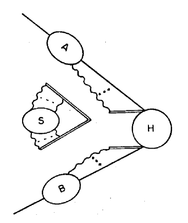
Figure 10: Basic factorization of form factor.

Our aim now is to construct a formula that exhibits the factorization of Fig. 10, that has explicit operator definitions of the factors, and that has no restrictions on the momenta of the lines in the Feynman graphs. First let us observe that, for example, the Feynman rules for both the jet-A subgraph and the eikonal line attached to it can be derived from the following matrix element of the quark field with a path-ordered exponential of the gluon field:

$$\left<0\left|T\exp\left[-ig\mu^{\epsilon}\int^{\infty}_{0}\mathop{{\rm d}z}\nolimits u_{B}\cdot A(-u_{B}z)\right]q(0)\right|p_{A}\right>.$$

Now consider the following quantity:

 

$${J_{A}\left(\frac{p_{A}\cdot n^{2}}{n^{2}};m,M,g,\mu\right)\equiv{}}$$

 

The numerator is the same as (36), except that we have replaced $u^{\mu}_{B}$ by a space-like vector $n^{\mu}\equiv u_{A}^{\mu}-u_{B}^{\mu}$. This has the effect of suppressing the contribution of momenta for which $|k^{-}|\gg|k^{+}|$, i.e., momenta collinear to $B$. The need for the vector $n^{\mu}$ to be a space-like rather than time-like will appear later. The denominator in (37) is necessary to cancel graphs, like Fig. 11, with eikonal self-interactions; these do not appear in Fig. 10. Finally, since we have removed all restrictions on loop momenta, there are ultra-violet divergences in graphs like Fig. 12; these we define to be cancelled by renormalization counterterms.

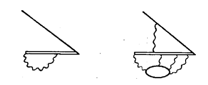
Figure 11: Typical graphs with eikonal self interactions.

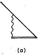
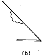
Figure 12: One loop graphs for $J_{A}$.

The one-loop contributions to $J_{A}$ are given in Fig. 12, so that

 

$${J_{A}={}}$$

 

This reproduces the contribution to Fig. 6 of the region where $k^{\mu}$ is collinear to $A$. In (38), $z_{2}$ is the residue of the pole of the quark propagator.

A jet-B factor may be defined similarly:

 

$${J_{B}\left(\frac{{p_{B}\cdot n}^{2}}{n^{2}};M,m,g,\mu\right)\equiv{}}$$

 

We now apply the same argument to $J_{A}$ and $J_{B}$ as the one we applied to obtain Fig. 10 from Fig. 7. The result has the form

 

$${J_{A}}$$

 

where “Jet-$A$” and “Jet-$B$” are the same quantities as in Fig. 10, but the soft and hard factors are different. Hence the form factor can be written

$$F(Q)=J_{A}\left(\frac{{p_{A}\cdot n}^{2}}{n^{2}}\right)\times J_{B}\left(\frac{{p_{B}\cdot n}^{2}}{n^{2}}\right)\times\hbox{soft}\times\hbox{hard}+O(1/Q^{2}).$$

We next recognize that the soft factor in Fig. 10 has the Feynman rules for

$$\left<0\left|T\exp\left[ig\mu^{\epsilon}\int^{\infty}_{0}\mathop{{\rm d}z}\nolimits\,u_{A}\cdot A\left(-zu^{\nu}_{A}\right)\right]\exp\left[-ig\mu^{\epsilon}\int^{\infty}_{0}\mathop{{\rm d}z}\nolimits\,u_{B}\cdot A\left(-zu^{\mu}_{B}\right)\right]\right|0\right>,$$

with the momenta restricted to the soft region. Suppose we were to define a soft factor as exactly (42) without any restrictions on loop momenta. Then there would be divergences from regions where gluons become collinear to $u_{A}$ or $u_{B}$. These divergences are caused by the fact that $u^{\mu}_{A}$ and $u^{\mu}_{B}$ are light-like and effectively represent an incoming quark and antiquark of infinitely high energy. An example is given by the one loop graph, Fig. 13:

$${ig^{2}\over(2\pi)^{4}}\int\mathop{{\rm d}^{4}k}\nolimits{N_{+-}(k)\over(k^{-}+i\epsilon)(m^{2}-k^{2})(k^{+}-i\epsilon)}.$$

The collinear divergences come from the regions where $k^{+}/k^{-}\to 0$ or $\infty$ with $k^{+}k^{-}$ fixed. They are evidently artificial divergences. The actual collinear regions of the original form factor have already been taken into account by the factors $J_{A}$ and $J_{B}$ in eq. (41), so we would also be guilty of double-counting if we were to keep exactly (42) as our definition of the soft factor. (There is also an ordinary ultraviolet divergence from the region where $|k^{\mu}|\to\infty$; we will deal with this separately.)

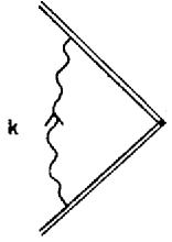
Figure 13: One loop graph for eq. (42).

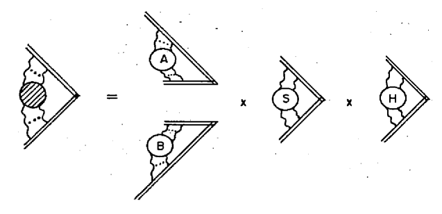
Figure 14: Factorization for eq. (42).

What we must do is to observe that the argument that led to the factorization of Fig. 10 for the form factor can also be applied to (42). The result is that the collinear parts factorize. This is shown in Fig. 14, where the soft factor is identical to the soft factor in eq. (41). Therefore we can write the original form factor as

$$F=J_{A}(p_{A}\cdot n^{2}/n^{2})J_{B}(p_{B}\cdot n^{2}/n^{2})S(M,m,g,\mu)\times{\rm hard}+O(1/Q^{2}),$$

where $S$ is the quantity (42) divided by its collinear divergences:

 

$${S}$$

 

This is represented by Fig. 15, and the last line in the equation has as its sole purpose the canceling of eikonal self-energies. In (45) we implicitly define UV divergences to be cancelled by renormalization counterterms.

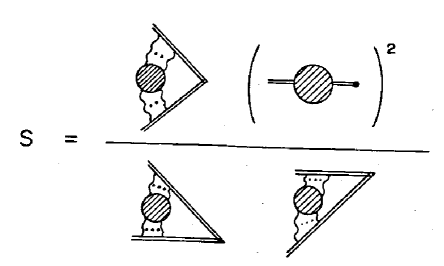
Figure 15: Definition of soft factor.

We finally observe that when the form factor $F$ is divided by $J_{A}J_{B}S$, all its collinear and soft regions have been cancelled. Hence we can define the hard factor by

$$H(Q,g,\mu)\equiv\lim_{\scriptstyle M\to 0\atop\scriptstyle m\to 0}F/(J_{A}J_{B}S).$$

Therefore we obtain the factorization

 

$${F(}$$

 

Here $J_{A}$, $J_{B}$, $S$ and $H$ are defined by Eqs. (37), (39), (45) and (46).

We cannot directly use this equation to control the $Q$-dependence of $F$. However, the dependence of $J_{A}$ and $J_{B}$ on $Q$ is through the vector $n^{\mu}$, since $Q^{2}=-4p_{A}\cdot n^{2}/n^{2}=-4p_{B}\cdot n^{2}/n^{2}$. What we will do in the next section is to compute the $Q$-dependence of $J_{A}$ and $J_{B}$ by differentiating each with respect to $n^{\mu}$, holding the physical momenta $p_{A}^{\mu}$ and $p_{B}^{\mu}$ fixed. The $Q$-dependence of $H$ will be renormalization-group controlled just as for the $Q$-dependent factor in $\phi^{3}$ theory.

The reason for using a spacelike vector $n^{\mu}$ can now be explained. On the various occasions that we factor out a soft region we needed to deform integrals over gluon momenta away from the Glauber region $|k^{+}k^{-}|\ll k_{T}^{2}$, just as in deriving eq. (33). For consistency all these deformations must be in the same direction. In the case of a soft region for the jet factors $J_{A}$ and $J_{B}$ this means that the $n\cdot k$ denominator must be $(k^{-}-k^{+}+i\epsilon)$ to give the same direction of deformation as in (33).

6 EVOLUTION EQUATION

In this section we will derive equations for the $Q$-dependence of the form factors, first in $(\phi^{3})_{6}$ theory and then in a gauge theory.

6.1 $(\phi^{3})_{6}$

The $Q$-dependence of the form factor (17) for $\phi^{3}$ theory is under renormalization-group control — see eq. (21) or (22). That is, after the factorization is obtained, we may change $\mu$ to different values in the two factors to eliminate all the large logarithms in their perturbation expansions. So we need not bother to derive an explicit equation for its $Q$-dependence. However, for the sake of the comparison with the case of a gauge theory, we will nevertheless do so.

From eq. (22) we have

 

$${{\partial\ln F\over\partial\ln Q}}$$

 

The right-hand side of this equation can be expanded in powers of $g$. The expansion contains no logarithms of $Q$ or of the masses, so it is valid to approximate it by the first term or two, provided only that $g(Q)$ is small. Since $\phi^{3}$ theory is asymptotically free, such an approximation is valid for all large enough values of $Q$. Indeed, given that ${}^{\ref{26}]}$

$${g^{2}(\mu)\over 64\pi^{3}}={4/3\over\ln(\mu^{2}/\Lambda^{2})}+O\left(\ln(\ln\mu)/\ln^{2}\mu\right),$$

we find that

$${\partial\ln F\over\partial\ln Q}={-4/3\over\ln\left(Q^{2}/\Lambda^{2}\right)}+\cdots.$$

Here we have used the value of $\tilde{\gamma}$ that can be extracted from the one-loop form factor (16):

 

$${\tilde{\gamma}}$$

 

Note that the calculation of $\tilde{\gamma}$ from the vertex graphs may be done entirely in the massless theory. This results in a saving of calculational effort.

Since the right-hand-side of (48) is of order $g^{2}(Q)$ with no extra logarithms of $Q$, the variation of the form factor for, say, a doubling of $Q$ is small, of order $1/\ln(Q/\Lambda)$. This is comparable to the scaling violations in deep-inelastic scattering. If we integrate over a wide range of $Q$, say from a value $Q_{0}$ to a value of order $Q_{0}^{2}/\Lambda$, effects of order unity arise. If both $Q/\Lambda$ and $Q_{0}/\Lambda$ are large, then

$$F(Q)=F(Q_{0})\left[{\ln(Q^{2}/\Lambda^{2})\over\ln(Q^{2}_{0}/\Lambda^{2})}\right]^{-2/3}\left[1+O\left(\ln\ln(Q_{0})/\ln(Q_{0})\right)\right].$$

These results will be used as a standard of comparison when we have derived the corresponding results for a gauge theory.

The accuracy of the results may be systematically improved by calculating higher orders in perturbation theory.

6.2 Gauge theory jet factors

In a gauge theory, the form factor satisfies the factorization equation (47). The hard (or ultra-violet) factor $H$ has $Q$-dependence that is renormalization group controlled, just as in $(\phi^{3})_{6}$ theory. But there is further $Q$-dependence in the jet factors. This comes essentially from the possibility of emission of gluons of moderate transverse momentum in a range of rapidity bounded by the two incoming particles. These gluons are divided into what we may term left-movers and right-movers by the vector $n_{\mu}$. The remaining contributions are put into the soft factor $S$ and the hard factor $H$. The details of the cut-off on rapidity given by the vector $n^{\mu}$ are incorrect in the central region of finite center-of-mass rapidity. The errors are compensated by the $Q$-independent factor $S$ if they correspond to quanta of low transverse momentum. Quanta of large transverse momentum are also included in all of the factors $J_{A}$, $J_{B}$ and $S$, but they are incorrectly approximated; the hard factor $H$ was defined to cancel these errors.

If we were to directly investigate the $Q$-dependence of the form factor, we would have to find its dependence on $p^{\mu}_{A}$ and $p^{\mu}_{B}$. We would have to trace the flow of these external momenta inside Feynman graphs, and this would be a hard task. (See Sen’s work ${}^{\ref{10},\ref{27}]}$ for details on how to do this.) But if, instead, we examine the factors $J_{A}$ and $J_{B}$, we see that their $Q$-dependence comes from dependence on $p_{A}\cdot n^{2}/n^{2}$ and $p_{B}\cdot n^{2}/n^{2}$ respectively. So it is sufficient to find their dependence on $n^{\mu}$. This is very much easier because it involves the result of differentiating in their definitions the path-ordered exponentials of the gluon field, with respect to direction. This gives a very simple result, as we will now see.

We have for $J_{A}$

$${\partial J_{A}\over\partial\ln Q}=\delta n^{\nu}{\partial J_{A}\over\partial n^{\nu}},$$

where $\delta n^{\mu}$ is a backward-pointing time-like vector, normalized so that $\delta n^{2}=-n^{2}$ and $n\cdot\delta n=0$. With our previous representation, where $n^{\mu}=u^{\mu}_{A}-u^{\mu}_{B}$, we have $\delta n^{\mu}=-u^{\mu}_{A}-u^{\mu}_{B}$. The light-like vectors $u^{\mu}_{A}$ and $u^{\mu}_{B}$ are defined by $u^{+}_{A}=u^{-}_{B}=1$, $u^{-}_{A}=u^{+}_{B}=u^{T}_{A}=u^{T}_{B}=0$.

The $Q$-dependence of $J_{B}$ is obtained by the opposite variation of $n^{\mu}$:

$${\partial J_{B}\over\partial\ln Q}=-\delta n^{\nu}{\partial J_{B}\over\partial n^{\nu}}.$$

Since this will result in an equation identical to that for the $Q$-dependence of $J_{A}$, we will restrict our attention to $J_{A}$.

The result of differentiating the path-ordered exponential with respect to its direction is

 

$${\delta n^{\nu}{\partial\over\partial n^{\nu}}}$$

 

where we used the canonical equal-time commutation relations of the gluon field to commute $A^{0}$ with $A^{3}$ and $\partial A^{3}/\partial t$ with $A^{3}$. The resulting Feynman rules for $\partial J_{A}/\partial\ln Q$ are exhibited in Fig. 16 and Fig. 17. The version shown in the second line of Fig. 16 comes from the second derivation which we now give.

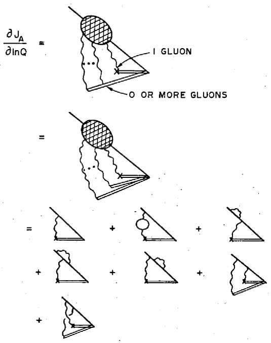
Figure 16: Equation for $J_{A}$.

$$= \left(ign^{\mu_{1}}\frac{i}{k_{1}\cdot n+i\epsilon}\right)\dots\left(ign^{\mu_{N}}\frac{i}{k_{1}\cdot n+\dots k_{N}\cdot n+i\epsilon}\right)$$

$$= \frac{g\,(\delta n\cdot k\,n^{\mu}-n\cdot k\,\delta n^{\mu})}{(k\cdot n+i\epsilon)^{2}}$$

Figure 17: Feynman rules for Fig. 16.

Suppose in a given Feynman graph (Fig. 18) for $J_{A}$ there are $N$ gluons attaching to the eikonal line. We have a factor

$${-gn^{\mu_{1}}\over(k_{1}\cdot n+i\epsilon)}\,{-gn^{\mu_{2}}\over(k_{1}\cdot n+k_{2}\cdot n+i\epsilon)}\cdots{-gn^{\mu_{N}}\over(k_{1}\cdot n+k_{2}\cdot n+\ldots k_{N}\cdot n+i\epsilon)}.$$

Now let us sum over all graphs which are the same as the first one except for having the $N$ gluons permuted. The result is to replace (56) by

$${-gn^{\mu_{1}}\over(k_{1}\cdot n+i\epsilon)}{-gn^{\mu_{2}}\over(k_{2}\cdot n+i\epsilon)}\ldots{-gn^{\mu_{N}}\over(k_{N}\cdot n+i\epsilon)},$$

and is illustrated in the left-hand side of Fig. 18. Finally, we take the derivative given on the right of eq. (53). This results in a derivative for each of the $N$ gluons, as symbolized in Fig. 16, each of the derivatives having the form

$${-g\Delta^{\mu}\over n\cdot k+i\epsilon}\equiv\delta n^{\nu}{\partial\over\partial n^{\nu}}\left({-gn^{\mu}\over n\cdot k+i\epsilon}\right)={g\over(k\cdot n+i\epsilon)^{2}}(\delta n\cdot k\,n^{\mu}-n\cdot k\,\delta n^{\mu}),$$

as stated in the Feynman rules, Fig. 17.

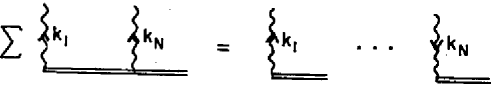
Figure 18: Sum over attachments to eikonal line gives eq. (57).

To derive an evolution equation we now use the same style of argument that we used to derive our first factorization (47). We can again divide momenta into collinear, soft and hard. (The collinear momenta here are only those collinear to $A$.) The simplification that now occurs is that a collinear momentum cannot enter the differentiated vertex. This is easy to see, since from (58) we find a factor

$$A\cdot\Delta={2k^{+}A^{-}-2k^{-}A^{+}\over k^{-}-k^{+}},$$

which is suppressed by a large factor compared with

$$A\cdot n=A^{-}-A^{+}$$

from a regular eikonal vertex. Here $k^{\mu}$ and $A^{\mu}$ are vectors collinear to $p_{A}^{\mu}$.

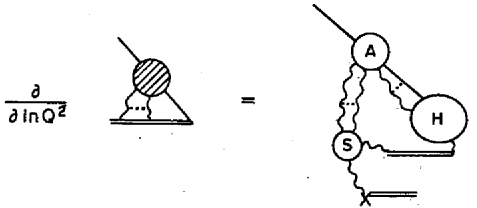
Figure 19: Leading regions for $J_{A}$.

Therefore, to leading twist, only soft and hard momenta attach to the differentiated vertex. The result is Fig. 19, which is analogous to Fig. 7 for the form factor.

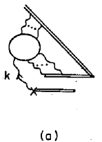
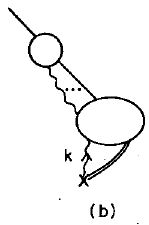
Figure 20: Factor obtained from Fig. 19 when $k$ is (a) soft, or (b) hard.

Whenever $k^{\mu}$ is soft we can use the Grammer-Yennie method to obtain the factor shown in Fig. 20(a). Whenever $k^{\mu}$ is hard its line disappears into a hard subgraph; then we apply the derivation of Fig. 9 to Fig. 20(b). This gives

$${\partial J_{A}\over\partial\ln Q}=J_{A}\times\left[{\rm soft}+{\rm hard}\right]+\hbox{higher twist}.$$

6.3 Operator form of jet evolution

It will be convenient to rewrite the soft factor in (61) so that it has an explicit definition in terms of a matrix element of an operator, just as we rewrote the jet and soft factors in Fig. 10 to give eq. (47). The same method of argument as for Fig. 10 gives

$${\partial\ln J_{A}\over\partial\ln Q}={1\over 2}K\left(m,M,\mu,g(\mu)\right)+{\rm hard}.$$

We have defined the soft term $K$ to have a factor $1/2$, since it will be multiplied by 2 when we write the evolution equation for the form factor $F$. Furthermore, this equation will have an extra hard term coming from the factor $H$ in eq. (47), so we do not bother to name the hard term in (62).

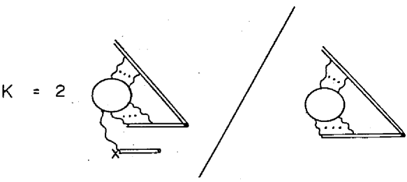
Figure 21: Definition of $K$.

The definition of the quantity $K$ is given in Fig. 21. It can be written as

 

$${K={}2}$$

 

No restriction is placed on the internal momenta of $K$, so we must add UV counterterms. Subdivergences in $K$ all correspond to the usual renormalizations of the interaction, and the remaining divergence is an overall divergence, so we must define it to be cancelled by an additive counterterm:

 

$${K(m,M,g,\mu)}$$

 

All soft contributions to $\partial\ln J_{A}/\partial\ln Q$ are contained in $K$ together with some hard contributions.

6.4 Gauge theory form factor

We can now write an equation for the form factor

$$\openup 6.45831pt\halign to=0.0pt{\hfil$\displaystyle{#}$ &$\displaystyle{{}#}$\hfil&\llap{$#$}\cr{\partial\ln F\over\partial\ln Q}&={\partial\ln J_{A}\over\partial\ln Q}+ {\partial\ln J_{B}\over\partial\ln Q}+{\partial\ln H\over\partial\ln Q}+ \hbox{higher twist} \cr&=K(m,M,g,\mu) + 2 \times\hbox{hard} + {\partial\ln H \over\partial\ln Q} +\hbox{higher twist} \cr&\equiv K(m,M,g,\mu)+G(Q/\mu;g)+\hbox{higher twist}. &\hbox to0.0pt{\hss$(65)\crcr}}$$

Since the dependence on masses has been separated from the dependence on $Q$ on the right-hand side of this equation, we will have an effective calculation of the large-$Q$ behavior of the form factor once we know the renormalization-group equation for $K$.

This equation is easy to derive, since $K_{\rm bare}$ is renormalization group invariant: $(\mu dK_{\rm bare}/d\mu=0)$. So from eq. (64) we find that

$$\openup 6.45831pt\halign to=0.0pt{\hfil$\displaystyle{#}$ &$\displaystyle{{}#}$\hfil&\llap{$#$}\cr\mu{\mathop{{\rm d}K}\nolimits\over\mathop{{\rm d}\mu}\nolimits}&=\mu{\mathop{{\rm d}}\nolimits\over\mathop{{\rm d}\mu}\nolimits}\delta K\cr&=\beta(g,\epsilon){\partial\delta K\over\partial g}\cr&\equiv-\gamma_{K}(g). &\hbox to0.0pt{\hss$(66)\crcr}}$$

The anomalous dimension $\gamma_{K}$ is finite at $\epsilon=0$, and if we use minimal subtraction, ’t Hooft’s methods ${}^{\ref{13}]}$ show that it is independent of $\epsilon$. The anomalous dimension of the form factor is zero, since the renormalized operator $[\bar{q}\gamma^{\mu}q]$ has zero anomalous dimension:

$$\mu{d\ln F\over d\mu}=0.$$

Thus eq. (65) gives the anomalous dimension of $G$:

 

$${\mu{d\over d\mu}G\left(Q/\mu;g(\mu)\right)}$$

 

We can now write the evolution equation in a form with no large logarithms:

$${\partial\ln F\over\partial\ln Q}=-\left[\int^{c_{2}Q}_{\mu}{\mathop{{\rm d}\mu^{\prime}}\nolimits\over\mu^{\prime}}\gamma_{K}\left(g(\mu^{\prime})\right)-G\left(1/c_{2};g(c_{2}Q)\right)-K\left(m,M,g(\mu),\mu\right)\right].$$

Here we displayed an overall factor $-1$, because the dominant term is the integral over the positive one-loop value of $\gamma_{K}$.

7 INTERPRETATION

The physical interpretation of eq. (69) and its derivation is as follows:

When the total energy $Q$ is increased, the phase space available increases for virtual quanta inside the form factor. Let us consider the size of the phase space split up into different ranges of transverse momentum. At low transverse momentum the range of phase-space is governed by the rapidity between the quark and antiquark — this gives the $K$ term. At large transverse momentum, of order $Q$, the quanta can only have finite rapidity, but the range of transverse momentum increases with $Q$ — this gives the $G$-term. Finally, the intermediate range is filled in by the anomalous-dimension term.

The precise form — e.g., the $Q$-independence of $K$ — and the detailed derivation rely on the fact that a particle (virtual or real) can only probe details of another particle (e.g. the initial quark or antiquark) if the relative rapidity is low. At large relative rapidity there is not sufficient proper time to get a detailed picture. Indeed the only elementary particle that can even interact at all across a large rapidity gap is the spin-1 gluon. Then it just measures the total charge and the direction of the probed particle. A coherent sum over the detailed structure is needed to give this result in perturbation theory, the result being formalized in the Ward identities. It is the need to sum over a set of Feynman graphs to get the physical answer that results in the technical complication of our derivation.

The key to understanding the derivation is to ask what happens to quanta inside the form factor when $Q$ is increased by boosting the quark and antiquark in opposite directions. We first examine quanta with transverse momenta much less than $Q$. The argument in the previous paragraph indicates that the interactions of these quanta with other quanta of very different rapidity, do not depend on the size of the rapidity gap. Thus the part of the change in $F$ that comes from quanta of low transverse momenta can be found by measuring the quanta that come into fill the interior of the increased rapidity range.

To make this measurement we first measure the contents of the incoming quark down to some finite rapidity, using the operator

$$\exp\left[ig\mu^{\epsilon}\int^{\infty}_{0}\mathop{{\rm d}z}\nolimits\,n\cdot A(nz)\right].$$

Then we differentiate with respect to $n^{\mu}$, to find the change caused by increasing the range of rapidity.

The remaining part of the variation of the form factor with $Q$ comes from the short-distance regime of large transverse momentum. This region is well understood.

8 SOLUTIONS AND CALCULATIONS

It is easy to solve eq. (69), with the result

 

$${F(Q)={}}$$

 

where $\hat{F}$ represents the effect of the initial condition for eq. (69), and is determined by the form factor at low $Q$. If $\mu$ is chosen to be of order the masses then this is a form in which no large logarithms appear in the coefficients of perturbation expansions; the logarithms in the unimproved perturbation series for $F$ are either explicitly in the exponent in (70) or are generated by the integration over $\mu^{\prime}$.

The leading logarithmic approximation to $F(Q)$ is obtained by using the result (see later) that $\gamma_{K}=g^{2}/(2\pi^{2})+O(g^{4})$ and by writing $g(\mu^{\prime})$ in terms of the running coupling, $g(\mu)$, at a fixed scale. Then the highest power of a logarithm of $Q$ is obtained from the lowest order term in the exponent. The result is

$$F=\exp\left[-{g^{2}\over 16\pi^{2}}\ln^{2}Q^{2}+\hbox{non-leading logs}\right].$$

In QCD, formulae like (70) can be derived for a number of important cases, such as the transverse-momentum distribution of the Drell-Yan process ${}^{\ref{4},\ref{5}]}$. Since QCD is asymptotically free, we can do an effective calculation from low orders of perturbation theory if $Q$ is large. Non-leading logarithmic corrections are thereby tamed.

8.1 Calculations

We now consider how to calculate the quantities $K$, $G$ and, particularly, $\gamma_{K}$ that appear in the exponent in (70) and on the right-hand side of the evolution equation (69). One method is to start from the Feynman graphs for the form factor. Then the results of these calculations are compared with the general form eq. (70). This determines $K$ and $G$ (and hence $\gamma_{K}$) except for an ambiguity of adding some function of $g$ to $K$ and subtracting the same function from $G$. This ambiguity is the same as the renormalization-scheme ambiguity for $K$ and $G$, and as such does not directly pertain to physics: the physics resides in the dependence of the functions $K$ and $G$ on their other arguments. Especially at higher-order this procedure is rather lengthy.

Now the terms in the exponent with the largest powers of logarithms are the most important — in particular the $\gamma_{K}$ term. So a short-cut can be made by calculating $K$. At two-loop order there is only one easy graph for $K$ — a vacuum polarization correction — but for the form factor there are five harder graphs. The anomalous dimension $\gamma_{K}$ is obtained from $K$ and in particular from its ultra-violet divergence.

In addition, the form (70) implies many relations between the logarithms of $Q$ in different orders. These are not manifest in a direct calculation. However their validity provides nontrivial tests of calculations. Nevertheless all the coefficients can be obtained by a direct calculation. For example, from an evaluation of the one-loop vertex, eq. (25), one can show that

$${\partial\ln F\over\partial\ln Q}=-{\alpha_{s}\over\pi}\ln\left(\frac{-Q^{2}}{m^{2}}\right)+O(\alpha_{\rm s}^{2})+\hbox{higher twist}.$$

This is evidently of the form of the evolution equation, eq. (65). It implies that

 

$${K}$$

 

where $C$ is a constant. The value of $C$ is not a priori fixed, and a change of the constant corresponds to a change of renormalization scheme for $K$. We choose to resolve the ambiguity by using $\overline{{\rm MS}}$ renormalization applied to a direct calculation of $K$ from its Feynman rules. Given that to 1-loop

 

$${K}$$

 

it is fairly easy to perform the integrals. The result, with $\overline{{\rm MS}}$ renormalization, is that

$$K={\alpha_{s}\over\pi}\ln\left(m^{2}/\mu^{2}\right)+O(\alpha_{\rm s}^{2}),$$

from which follows

$$\gamma_{K}=2{\alpha_{s}\over\pi}+O(\alpha_{\rm s}^{2}).$$

It is left as an exercise for the reader to show that the sole 2-loop graph gives the $O(\alpha_{\rm s}^{2})$ term in $\gamma_{K}$:

$$\gamma_{K}=2{\alpha_{s}\over\pi}-{10\over 9}\left({\alpha_{s}\over\pi}\right)^{2}+O\left(\alpha_{\rm s}^{3}\right).$$

There is a lot of information in these results, even without the two-loop result (77). For example, let us expand $\,\ln F$ in powers of $t=\ln(-Q^{2}/\mu^{2})$

 

$${\ln F={}}$$

 

where the coefficients may depend on $m$, $M$ and $\mu$, but not on $Q$. The leading logarithm results imply that $C_{24}=0$. Our formula (65) implies considerably more. Now, from (78) we have

 

$${{\partial\ln F\over\partial\ln Q}={}}$$

 

In order that $G$ in eq. (65) be independent of the masses $m$ and $M$, $C_{12}$, $C_{23}$ and $C_{22}$ must be independent of $m$ and $M$ (and hence of $\mu$). Furthermore, once one puts in the one-loop values, the requirement that $G$ satisfies its renormalization group equation implies that

$$C_{23}=-{1\over 36}.$$

Hence the new information for the form factor $F$ at 2 loops is 2 logarithms down from the leading logarithm, i.e. it is in $C_{22}$ and the less leading coefficients, $C_{21}$ and $C_{20}$. The double logarithm coefficient $C_{22}$ is related to the two-loop term in $\gamma_{K}$, given in eq. (77); this was the result of a relatively easy calculation. Hence

$$C_{22}={5\over 36}.$$

The remaining information, for which a full two-loop calculation of the form factor is needed, is in the terms with one and no logarithms of $Q$. These are three and four logarithms down from the leading $\ln^{4}Q$ term.

8.2 Comparison with other work

One can verify (77) and (80) from the calculation of Barbieri et al. ${}^{\ref{28}]}$. Note that in this calculation one must change renormalization prescription first.

Korthals-Altes and de Rafael ${}^{\ref{29}]}$ made a conjecture about an evolution equation for the form factor we are discussing. Their conjecture is that $(Q\,\partial/\partial Q-\beta\,\partial/\partial\alpha_{\rm s})\ln F$ is linear in $\ln Q$. It can be checked that their conjecture is implied by our eq. (69). However the converse is not true: Their conjectured result does not imply our eq. (65) with its specific dependences on masses.

A number of calculations of comparable quantities in QCD have been made. As will be discussed below, generalizations of our formulae apply not only to a simple quark form factor but notably also to the transverse momentum distribution in the Drell-Yan process and to two-hadron-inclusive production in ${{\rm e}^{+}{\rm e}^{-}}$ annihilation. (This last includes the energy-energy correlation as a special case.) The anomalous dimension $\gamma_{K}$ is common to all these processes.

The electromagnetic form factor of a quark in massless QCD also satisfies our equation (65) or (69), as shown by Sen ${}^{\ref{10}]}$. The coefficients are now

 

$${K}$$

 

Here $n_{f}$ is the number of quark flavors, while $T_{F}$, $C_{F}$ and $C_{A}$ are the usual group theory coefficients. ($T_{F}=\frac{1}{2}$, $C_{F}=\frac{4}{3}$ and $C_{A}=3$ for QCD, while $T_{F}=1$, $C_{F}=1$ and $C_{A}=0$ for QED.) Since there are no masses, $K_{\rm bare}$ is zero, and the renormalized $K$ equals its $\overline{{\rm MS}}$ counterterm. The resulting pole, as displayed in eq. (82), represents the infra-red divergence in $K$. Those terms that appear in the abelian case are given by our earlier calculations. The only purely nonabelian term in the order to which we work in eq. (82) is the two-loop $C_{F}C_{A}$ term. We have deduced its value from ${}^{\ref{30},\ref{31},\ref{32}]}$, as I will explain later.

The calculation in QCD that can most directly be compared with eq. (82) is by Gonsalves ${}^{\ref{33}]}$ who has calculated precisely the quark form factor in QCD, at two-loop order. (The purpose of doing this is that one can use the deduced value of $\gamma_{K}$ in other processes.) Gonsalves’ results do not obey the correct evolution equation, which should hold in QCD as well in QED. Note that his renormalization prescription differs in detail from both $\overline{{\rm MS}}$ and MS. The agreement between the other calculations indicates that there must be an error in Gonsalves’ calculation.

8.3 Infrared divergences in QCD

Korchemskii and Radyushkin ${}^{\ref{30},\ref{34}]}$ have studied the infrared divergences of the electromagnetic form factor of a quark in QCD at large $Q$. (Their ultimate aim ${}^{\ref{35}]}$ is to study the full Sudakov problem in QCD.) Consequently their methods have much in common with the work described in this paper. Indeed their results are written in terms of path-ordered exponentials that are similar to the ones used in this article. Moreover they have derived the necessary generalization of the Grammer-Yennie method to the nonabelian case.

In an abelian theory, the infrared divergences (as the gluon mass goes to zero) are rather simple: they form a factor which is the exponential of the one loop infrared divergence. In eq. (69), for the $Q$-dependence of the form factor, all the infrared divergences are in the term $K$. Gluon self couplings in an abelian theory are induced solely by quark loops, and these loops are suppressed when the gluon momenta go to zero and the quark mass is nonzero. Hence only the one loop part of $\gamma_{K}$ is needed for the calculation of the infrared divergences in the abelian theory.

In QCD the infrared divergences are much more complicated, since the gluon self couplings are not so suppressed at zero momentum. Korchemskii and Radyushkin show that the infrared divergences form a factor:

$${\cal M}_{\rm soft}\equiv\langle 0|T\bar{P}\exp[-ig\int_{0}^{\infty}\mathop{{\rm d}s}\nolimits\,p_{A}^{\mu}A_{\mu}(p_{A}s)]\,P\exp[ig\int_{0}^{\infty}\mathop{{\rm d}s}\nolimits\,p_{B}^{\mu}A_{\mu}(p_{B}s)]|0\rangle_{\rm IR}.$$

The subscript ‘IR’ means that integrations are restricted to the infra-red region. When $Q^{2}\equiv(p_{A}-p_{B})^{2}$ gets large, the infra-red behavior is governed by the anomalous dimension of the cusp, $\Gamma_{\rm cusp}$. The ability to do systematic perturbative calculations at large $Q$ relies on the property, proved by Korchemskii and Radyushkin, that $\Gamma_{\rm cusp}$ is linear in $\ln(Q)$ for large $Q$:

$$\Gamma_{\rm cusp}=A(\alpha_{\rm s})\ln(Q/M)+B(\alpha_{\rm s})+O(1/Q^{2}).$$

This linearity is implied by our results (if it is assumed that they extend to QCD). Indeed $A(\alpha_{\rm s})$ in eq. (84) is the same as our $\gamma_{K}$. The proof is simple:

 

$${{\partial\over\partial\ln Q^{2}}\Gamma_{\rm cusp}}$$

 

Here we have employed the factorization theorem for $\ln{\cal M}_{\rm soft}$ that is analogous to the one for the quark form factor. The soft term $K$ is the same as for the form factor. But the hard term $G_{\rm KR}$ is different. Indeed, since it is a pure ultraviolet quantity, with no scale dependence, it is zero.

This result enables us to obtain the non-abelian part of $\gamma_{K}$ at two loop order; this is the term in eq. (82) that is proportional to $C_{F}C_{A}$. Since Korchemskii and Radyushkin investigate the infrared divergences of the form factor with massive quarks, they cannot calculate the $C_{F}T_{F}$ term.

8.4 Other QCD calculations

Kodaira and Trentadue ${}^{\ref{32}]}$ considered the energy-energy correlation in ${{\rm e}^{+}{\rm e}^{-}}$ annihilation. They worked with a different formalism for the Sudakov form factor. Their calculation was the first from which the nonabelian part of the two-loop value for $\gamma_{K}$ can be deduced. They also agree with the abelian part, as calculated directly from $K$.

Davies and Stirling ${}^{\ref{31}]}$ have calculated the Drell-Yan cross section at order $\alpha_{\rm s}^{2}$. They deduce $\gamma_{K}$ and the equivalent of $K$ and $G$. They confirm the value for $\gamma_{K}$ given in eq. (82).

9 APPLICATIONS TO QCD

As has already been noted, there are many cases in QCD where something like a Sudakov form factor enters. The most straightforward extension of the results in this article is to transverse momentum distributions. The transverse-momentum $q_{T}$ is a third important scale for the cross-section, in addition to the total energy $Q$ and the hadron mass-scale. Two logarithms of $Q/q_{T}$ per loop are present in Feynman graphs.

In the case of two-particle inclusive cross-sections in ${{\rm e}^{+}{\rm e}^{-}}$ annihilation, Collins and Soper ${}^{\ref{4}]}$ derived an equation generalizing Eqs. (65) and (69). The same anomalous dimension $\gamma_{K}$ makes its appearance. Technically the main difference between ${}^{\ref{4}]}$ and the treatment in the present article, aside from having a non-abelian gauge group, was that there we used an axial gauge $n\cdot A=0$ instead of Feynman gauge. This resulted in a nice simplification. For example, in eq. (37), the line integral of the gluon field is zero, so that in ${}^{\ref{4}]}$ the definition of $J_{A}$ would have been

$$J_{A}\left(P_{A}\cdot n^{2}/n^{2}\right)=\left<0|q(0)|P_{A}\right>_{\rm axial\ gauge},$$

with the dependence on $n^{\mu}$ now being a dependence on the choice of gauge.

My treatment of the Sudakov form factor in ${}^{\ref{21}]}$ used Coulomb gauge, which behaves for this purpose rather like the axial gauge. In either gauge, explicit Feynman graph calculations are made more difficult than in covariant gauge by the complicated form of the numerator of the gluon propagator. In axial gauge we have

$$N^{\rm axial}_{\mu\nu}=\left\{g_{\mu\nu}-{n_{\mu}k_{\nu}+k_{\mu}n_{\nu}\over n\cdot k}+{k_{\mu}k_{\nu}n^{2}\over k\cdot n^{2}}\right\}_{\rm PV},$$

where ‘PV’ denotes the principal-value prescription for the singularities at $n\cdot k=0$. In Coulomb gauge, we have

$$N^{\rm Coulomb}_{\mu\nu}=g_{\mu\nu}-{(\delta n_{\mu}k_{\nu}+k_{\mu}\delta n_{\nu})\,\delta n\cdot k\over-k^{2}\delta n^{2}+(\delta n\cdot k)^{2}}+{k_{\mu}k_{\nu}\delta n^{2}\over-k^{2}\delta n^{2}+\delta n\cdot k^{2}},$$

where $\delta n^{\mu}$ is the vector defined just below eq. (53).

However, there are more fundamental disadvantages than calculational complexity to use of these physical gauges. It is very hard to define higher order graphs in the axial gauge because of the need to multiply principal values. To overcome this, considerable complication in the Feynman rules is necessary ${}^{\ref{36}]}$, and the simplicity of the Ward identities is no longer clear. There are also complications in the Feynman rules in Coulomb gauge beyond 2-loop order ${}^{\ref{37}]}$. In both cases, it is not clear that a complete and correct all-orders derivation can be given easily.

We expect corresponding results to the ones for the energy-energy correlation to hold for the Drell-Yan process; they have been formulated by Collins, Soper and Sterman ${}^{\ref{5}]}$. This work, because it entails a complete treatment of a factorization theorem for a process at low transverse momentum, includes treatment of intrinsic transverse momentum within QCD. In other work of that period, based on leading logarithmic formulations, intrinsic transverse momentum tends to appear as an ad hoc phenomenological modification to the basic formula for the cross section.

Davies and Stirling ${}^{\ref{6},\ref{31}]}$ have applied this formalism phenomenologically. Altarelli et al. ${}^{\ref{7}]}$ have also performed phenomenological calculations, but without the full treatment of the intrinsic transverse momentum effects.

A further disadvantage to using the physical gauges appears ${}^{\ref{1}]}$ when we try to derive results for the Drell-Yan cross-section. The problem is that singularities in the numerators of the gluon propagators (87) or (88) wreck the derivation of the form of the leading regions. Specifically, we need contour-deformation arguments generalizing those which we summarized at the end of Sec. 5, and these are invalid in an axial or Coulomb gauge. So Collins, Soper and Sterman ${}^{\ref{1}]}$ were forced to the use of a covariant gauge, at the price of some extra technicalities in the proofs. At the same time, the proofs come out to be cleaner. It is a generalization of the method of ${}^{\ref{1}]}$ that is used in the present article.

Another line of development comes from realizing that similar physical phenomena to those in the Sudakov form factor occur inside of amplitudes for scattering in the Regge region. Sen ${}^{\ref{27}]}$ has produced very important results in this area. He used Coulomb gauge.

ACKNOWLEDGEMENTS

This work was supported in part by the U.S. Department of Energy, Division of High Energy Physics, contracts W-31-109-ENG-38 and DE-FG02-85ER-40235, and also by the National Science Foundation, grants Phy-82-17853 and Phy-85-07627, supplemented by funds from the National Aeronautics and Space Administration. I wish to thank the Institutes for Theoretical Physics at Santa Barbara and Stony Brook for their hospitality during part of the preparation of this article.

REFERENCES

1. J.C. Collins, D.E. Soper and G. Sterman, Nucl. Phys. B261, 104 (1985) and B308, 833 (1988); G. Bodwin, Phys. Rev. D31, 2616 (1985) and D34, 3932 (1986). These papers give the fullest proofs of factorization in the case of the Drell-Yan and other processes in hadron-hadron scattering. See also Ref. 2 for inclusive ${{\rm e}^{+}{\rm e}^{-}}$ cross sections, and Ref. 38 for the original papers. A summary is given in the article by Collins, Soper and Sterman in this volume.

2. J.C. Collins and G. Sterman, Nucl. Phys. B185, 172 (1981).

3. V. Sudakov, Zh. Eksp. Teor. Fiz. 30, 87 (1956); (Eng. trans) Sov. Phys. JETP 3, 65 (1956).

4. J.C. Collins and D.E. Soper, Nucl. Phys. B193, 381 (1981), and Nucl. Phys. B197, 446 (1982).

5. J.C. Collins, D.E. Soper and G. Sterman, Nucl. Phys. B250, 199 (1985); J.C. Collins and D.E. Soper, “Parton transverse momentum”, in “Lepton Pair Production” ed. J. Tran Thanh Van (Editions Frontières, Dreux, 1981).

6. C.T.H. Davies, B.R. Webber and W.J. Stirling, Nucl. Phys. B256, 413 (1985).

7. G. Altarelli, R.K. Ellis, M. Greco and G. Martinelli, Nucl. Phys. B246, 12 (1984).

8. Yu.L. Dokshitzer, D.I. Dyakonov and S.I. Troyan, Phys. Reports 58, 269 (1980).

9. G. Parisi and R. Petronzio, Nucl. Phys. B154, 427 (1979).

10. A. Sen, Phys. Rev. D24, 3281 (1981).

11. S. Libby and G. Sterman, Phys. Rev. D18, 3252, 4737 (1978).

12. S. Coleman and R.E. Norton, Nuovo Cim. 28, 438 (1965).

13. G. ’t Hooft, Nucl. Phys. B61, 455 (1973).

14. W.A. Bardeen, A.J. Buras, D.W. Duke and T. Muta, Phys. Rev. D18, 3998 (1978).

15. M. Creutz and L.-L. Wang, Phys. Rev. D10, 3749 (1974); S.-S. Shei, Phys. Rev. D11, 164 (1975); P. Menotti, Phys. Rev. D11, 2828 (1975).

16. See any good modern textbook on field theory, e.g., G. Itzykson and J.-B. Zuber, “Quantum Field Theory” (McGraw-Hill, New York, 1980), or see J.C. Collins, “Renormalization” (Cambridge University Press, Cambridge, 1984).

17. E.g. D. Gross in “Methods in Field Theory” (eds. R. Balian and J. Zinn-Justin) (North-Holland, Amsterdam, 1976), or Collins, Ref. 16.

18. G. Grunberg, Phys. Lett. 95B, 70 (1980) and Phys. Rev. D29, 2315 (1984); P.M. Stevenson, Phys. Rev. D23, 2916 (1981) and Nucl. Phys. B203, 472 (1982); D.W. Duke and R.G. Roberts, Phys. Reports 120, 275 (1985).

19. R. Jackiw, Ann. Phys. (N.Y.) 48, 292 (1968).

20. A.H. Mueller, Phys. Rev. D20, 2037 (1979).

21. J.C. Collins Phys. Rev. D22, 1478 (1980).

22. J.C. Collins, Argonne preprint ANL-HEP-PR-84-36.

23. J.D. Bjorken and S.D. Drell, “Relativistic Quantum Fields” (McGraw-Hill, New York, 1966).

24. G. Grammer and D. Yennie, Phys. Rev. D8, 4332 (1973).

25. G. Bodwin, S.J. Brodsky and G.P. Lepage, Phys. Rev. Lett. 47, 1799 (1981).

26. A.J. Macfarlane and G. Woo, Nucl. Phys. B77, 91 (1974).

27. A. Sen, Phys. Rev. D27, 2997 (1983) and D28, 860 (1983).

28. R. Barbieri, J.A. Mignaco and E. Remiddi, Nuovo Cim. 11A, 824 (1972).

29. C.P. Korthals-Altes and E. de Rafael, Nucl. Phys. B106, 237 (1976).

30. G.P. Korchemskii and A.V. Radyushkin, Yad. Fiz. 45, 1466 (1987) [Eng. transl.: Sov. J. Nucl. Phys. 45, 910 (1987)].

31. C.T.H. Davies and W.J. Stirling, Nucl. Phys. B244, 337 (1984).

32. J. Kodaira and L. Trentadue, Phys. Lett. 112B, 66 (1982).

33. R.J. Gonsalves, Phys. Rev. D28, 1542 (1983).

34. S.V. Ivanov, G.P. Korchemskii and A.V. Radyushkin, Yad. Fiz. 44, 230 (1986) [Eng. transl: Sov. J. Nucl. Phys. 44, 145 (1986)].

35. G.P. Korchemskii, “Double Logarithmic Asymptotics in QCD”, Dubna preprint E2-88-600, and “Sudakov Form Factor in QCD”, Dubna preprint E2-88-628.

36. P.V. Landshoff, Phys. Lett. 169B, 69 (1986), and references therein.

37. P.J. Doust and J.C. Taylor, Phys. Lett. 197B, 232 (1987).

38. D. Amati, R. Petronzio, and G. Veneziano, Nucl. Phys. B140, 54 (1978) and B146, 29 (1978); R.K. Ellis, H. Georgi, M. Machacek, H.D. Politzer, and G.G. Ross, Nucl. Phys. B152, 285 (1979); A.V. Efremov and A.V. Radyushkin, Teor. Mat. Fiz. 44, 17 (1980) [Eng. transl.: Theor. Math. Phys. 44, 573 (1981)], Teor. Mat. Fiz. 44, 157 (1980) [Eng. transl.: Theor. Math. Phys. 44, 664 (1981)], Teor. Mat. Fiz. 44, 327 (1980) [Eng. transl.: Theor. Math. Phys. 44, 774 (1981)]; Libby and Sterman, Ref. 11.