Event shapes in $\boldsymbol{e^{+}e^{-}}$ annihilation and deep inelastic scattering

Abstract

This article reviews the status of event-shape studies in $e^{+}e^{-}$ annihilation and DIS. It includes discussions of perturbative calculations, of various approaches to modelling hadronisation and of comparisons to data.

1 Introduction

Event shape variables are perhaps the most popular observables for testing QCD and for improving our understanding of its dynamics. Event shape studies began in earnest towards the late seventies as a simple quantitative method to understand the nature of gluon bremsstrahlung [1, 2, 3, 4, 5]. For instance, it was on the basis of comparisons to event shape data that one could first deduce that gluons were vector particles, since theoretical predictions employing scalar gluons did not agree with experiment [6].

Quite generally, event shapes parametrise the geometrical properties of the energy-momentum flow of an event and their values are therefore directly related to the appearance of an event in the detector. In other words the value of a given event shape encodes in a continuous fashion, for example, the transition from pencil-like two-jet events with hadron flow prominently distributed along some axis, to planar three-jet events or events with a spherical distribution of hadron momenta. Thus they provide more detailed information on the final state geometry than say a jet finding algorithm which would always classify an event as having a certain finite number of jets, even if the actual energy flow is uniformly distributed in the detector and there is no prominent jet structure present in the first place.

Event shapes are well suited to testing QCD mainly because, by construction, they are collinear and infrared safe observables. This means that one can safely compute them in perturbation theory and use the predictions as a means of extracting the strong coupling $\alpha_{s}$. They are also well suited for determinations of other parameters of the theory such as constraining the quark and gluon colour factors as well as the QCD beta function. Additionally they have also been used in other studies for characterising the final state, such as investigations of jet and heavy quark multiplicities as functions of event shape variables [7, 8].

Aside from testing the basic properties of QCD, event shape distributions are a powerful probe of our more detailed knowledge of QCD dynamics. All the commonly studied event shape variables have the property that in the region where the event shape value is small, one is sensitive primarily to gluon emission that is soft compared to the hard scale of the event and/or collinear to one of the hard partons. Such small-transverse-momentum emissions have relatively large emission probabilities (compared to their high transverse momentum counterparts) due to logarithmic soft-collinear dynamical enhancements as well as the larger value of their coupling to the hard partons. Predictions for event shape distributions therefore typically contain large logarithms in the region where the event-shape is small, which are a reflection of the importance of multiple soft and/or collinear emission. A successful prediction for an event shape in this region requires all-order resummed perturbative predictions or the use of a Monte-Carlo event generator, which contains correctly the appropriate dynamics governing multiple particle production. Comparisons of these predictions to experimental data are therefore a stringent test of the understanding QCD dynamics that has been reached so far.

One other feature of event shapes, that at first appeared as an obstacle to their use in extracting the fundamental parameters of QCD, is the presence of significant non-perturbative effects in the form of power corrections that vary as an inverse power of the hard scale, $(\Lambda/Q)^{2}p$. For most event shapes, phenomenologically it was found that $p=1/2$ (as discussed in [9]), and the resulting non-perturbative effects can be of comparable size to next-to-leading order perturbative predictions, as we shall discuss presently. The problem however, can be handled to a large extent by hadronisation models embedded in Monte-Carlo event generators [10, 11, 12], which model the conversion of partons into hadrons at the cost of introducing several parameters that need to be tuned to the data. Once this is done, application of such hadronisation models leads to very successful comparisons of perturbative predictions with experimental data with, for example, values of $\alpha_{s}$ consistent to those obtained from other methods and with relatively small errors.

However since the mid-nineties attempts have also been made to obtain a better insight into the physics of hadronisation and power corrections in particular. Theoretical models such as those based on renormalons have been developed to probe the non-perturbative domain that gives rise to power corrections (for a review, see [13]). Since the power corrections are relatively large effects for event shape variables, scaling typically as $1/Q$ (no other class of observable shows such large effects), event shapes have become the most widely used means of investigating the validity of these ideas. In fact an entire phenomenology of event shapes has developed which is based on accounting for non-perturbative effects via such theoretically inspired models, and including them in fits to event shape data alongside the extraction of other standard QCD parameters. In this way event shapes also serve as a tool for understanding more quantitatively the role of confinement effects.

The layout of this article is as follows. In the following section we list the definitions of several commonly studied event shapes in $e^{+}e^{-}$ annihilation and deep inelastic scattering (DIS) and discuss briefly some of their properties. Then in section 3 we review the state of the art for perturbative predictions of event-shape mean values and distributions. In particular, we examine the need for resummed predictions for distributions and clarify the nomenclature and notation used in that context, as well as the problem of matching these predictions to fixed order computations. We then turn, in sections 4 and 5, to comparisons with experimental data and the issue of non-perturbative corrections, required in order to be able to apply parton level calculations to hadronic final state data. We discuss the various approaches used to estimate non-perturbative corrections, ranging from phenomenological hadronisation models to analytical approaches based on renormalons, and shape-functions. We also discuss methods where the standard perturbative results are modified by use of renormalisation group improvements or the use of ‘dressed gluons’. We study fits to event shape data, from different sources, in both $e^{+}e^{-}$ annihilation and DIS and compare the various approaches that are adopted to make theoretical predictions. In addition we display some of the results obtained by fitting data for various event shape variables for parameters such as the strong coupling, the QCD colour factors and the QCD beta function. Lastly, in section 6, we present an outlook on possible future developments in the field.

2 Definitions and properties

We list here the most widely studied event shapes, concentrating on those that have received significant experimental and theoretical attention.

2.1 $e^{+}e^{-}$

The canonical event shape is the thrust [14, 2], $T$:

$$T=\max_{\vec{n}_{T}}\frac{\sum_{i}|\vec{p}_{i}.\vec{n}_{T}|}{\sum_{i}|{\vec{p}}_{i}|}\,,$$ (1)

where the numerator is maximised over directions of the unit vector $\vec{n}_{T}$ and the sum is over all final-state hadron momenta $p_{i}$ (whose three-vectors are ${\vec{p}}_{i}$ and energies $E_{i}$). The resulting $\vec{n}_{T}$ is known as the thrust axis. In the limit of two narrow back-to-back jets $T\to 1$, while its minimum value of $1/2$ corresponds to events with a uniform distribution of momentum flow in all directions. The infrared and collinear safety of the thrust (and other event shapes) is an essential consequence of its linearity in momenta. Often it is $1-T$ (also called $\tau$) that is referred to insofar as it is this that vanishes in the $2$-jet limit.

A number of other commonly studied event shapes are constructed employing the thrust axis. Amongst these are the invariant squared jet-mass [15] and the jet-broadening variables [16], defined respectively as

$$\rho_{\ell,r} = \frac{\left(\sum_{i\in{\cal H}_{\ell,r}}p_{i}\,\right)^{2}}{\left(\sum_{i}E_{i}\right)^{2}}\,,$$ (2)

$$B_{\ell,r} = \frac{\sum_{i\in{\cal H}_{\ell,r}}|{\vec{p}}_{i}\times\vec{n}_{T}|}{2\sum_{i}|{\vec{p}}_{i}|}\,,$$ (3)

where the plane perpendicular to the thrust axis is used to separate the event into left and right hemisphere, ${\cal H}_{\ell}$ and ${\cal H}_{r}$. Given these definitions one can study the heavy-jet mass, $\rho_{H}=\max(\rho_{\ell},\rho_{r})$ and wide-jet broadening, $B_{W}=\max(B_{\ell},B_{r})$; analogously one defines the light-jet mass ($\rho_{L}$) and narrow-jet broadening $B_{N}$; finally one defines also the sum of jet masses $\rho_{S}=\rho_{\ell}+\rho_{r}$ and the total jet broadening $B_{T}=B_{\ell}+B_{r}$ and their differences $\rho_{D}=\rho_{H}-\rho_{L}$, and $B_{D}=B_{W}-B_{N}$. Like $1-T$, all these variables (and those that follow) vanish in the two-jet limit; $\rho_{L}$ and $B_{N}$ are special in that they also vanish in the limit of three narrow jets (three final-state partons; or in general for events with any number of jets in the heavy hemisphere, but only one in the light hemisphere).

Another set of observables [17] making use of the thrust axis starts with the thrust major $T_{M}$,

$$T_{M}=\max_{{\vec{n}}_{M}}\frac{\sum_{i}|\vec{p}_{i}.\vec{n}_{M}|}{\sum_{i}|{\vec{p}}_{i}|}\,,\qquad\quad\vec{n}_{M}.\vec{n}_{T}=0\,,$$ (4)

where the maximisation is performed over all directions of the unit vector $\vec{n}_{M}$, such that $\vec{n}_{M}.\vec{n}_{T}=0$. The thrust minor, $T_{m}$, is given by

$$T_{m}=\frac{\sum_{i}|\vec{p}_{i}.\vec{n}_{m}|}{\sum_{i}|{\vec{p}}_{i}|}\,,\qquad\qquad\vec{n}_{m}=\vec{n}_{T}\times\vec{n}_{M}\,,$$ (5)

and is sometimes also known [18] as the (normalised) out-of-plane momentum $K_{\mathrm{out}}$. Like $\rho_{L}$ and $B_{N}$, it vanishes in the three-jet limit (and, in general, for planar events). Finally from $T_{M}$ and $T_{m}$ one constructs the oblateness, $O=T_{M}-T_{m}$.

An alternative axis is used for the spherocity $S$ [2],

$$S=\left(\frac{4}{\pi}\right)^{2}\max_{\vec{n}_{S}}\left(\frac{\sum_{i}|\vec{p}_{i}\times\vec{n}_{S}|}{\sum_{i}|{\vec{p}}_{i}|}\right)^{2}.$$ (6)

While there exist reliable (though algorithmically slow) methods of determining the thrust and thrust minor axes, the general properties of the spherocity axis are less well understood and consequently the spherocity has received less theoretical attention. An observable similar to the thrust minor (in that it measures out-of-plane momentum), but defined in a manner analogous to the spherocity is the acoplanarity [19], which minimises a (squared) projection perpendicular to a plane.

It is also possible to define event shapes without reference to an explicit axis. The best known examples are the $C$ and $D$ parameters [20] which are obtained from the momentum tensor [21]

$$\Theta_{ab}=\left(\sum_{i}\frac{p_{ai}p_{bi}}{|\vec{p}_{i}|}\right)/\sum_{i}|{\vec{p}}_{i}|\,,$$ (7)

where $p_{ai}$ is the $a^{\mathrm{th}}$ component of the three vector $\vec{p}_{i}$. In terms of the eigenvalues $\lambda_{1}$, $\lambda_{2}$ and $\lambda_{3}$ of $\Theta_{ab}$, the $C$ and $D$ parameters are given by

$$C=3(\lambda_{1}\lambda_{2}+\lambda_{2}\lambda_{3}+\lambda_{3}\lambda_{1})\,,\qquad\quad D=27\lambda_{1}\lambda_{2}\lambda_{3}\,.$$ (8)

The $C$-parameter is related also to one of a series of Fox-Wolfram observables [4], $H_{2}$, and is sometimes equivalently written as

$$C=\frac{3}{2}\frac{\sum_{i,j}|{\vec{p}}_{i}||{\vec{p}}_{j}|\sin^{2}\theta_{ij}}{\left(\sum_{i}|{\vec{p}}_{i}|\right)^{2}}\,.$$ (9)

The $D$-parameter, like the thrust minor, vanishes for all final-states with up to 3 particles, and in general, for planar events.

The $C$-parameter can actually be considered (in the limit of all particles being massless) as the integral of a more differential observable, the Energy-Energy Correlation (EEC) [5],

$$\frac{d\Sigma(\chi)}{d\cos\chi} = \frac{d\sigma}{\sigma\,d\cos\chi}=\langle\,\mathrm{EEC}(\chi)\,\rangle$$ (10)

$$\mathrm{EEC}(\chi) = \frac{\sum_{i,j}E_{i}E_{j}\delta(\cos\chi-\cos\theta_{ij})}{\left(\sum_{i}E_{i}\right)^{2}}$$ (11)

where the average in eq. (10) is carried out over all events.

Another set of variables that characterise the shape of the final state are the $n$-jet resolution parameters that are generated by jet finding algorithms. Examples of these are the JADE [24] and Durham [25] jet clustering algorithms. One introduces distance measures $y_{ij}$

$$y_{ij}^{(\mathrm{Jade})} = \frac{2E_{i}E_{j}(1-\cos\theta_{ij})}{(\sum_{k}E_{k})^{2}},$$ (12)

$$y_{ij}^{(\mathrm{Durham})} = \frac{2\,\mathrm{min}(E_{i}^{2},E_{j}^{2})(1-\cos\theta_{ij})}{(\sum_{k}E_{k})^{2}},$$ (13)

for each pair of particles $i$ and $j$. The pair with the smallest $y_{ij}$ is clustered (by adding the four-momenta — the $E$ recombination scheme) and replaced with a single pseudo-particle; the $y_{ij}$ are recalculated and the combination procedure repeated until all remaining $y_{ij}$ are larger than some value $y_{\mathrm{cut}}$. The event-shapes based on these jet algorithms are $y_{3}\equiv y_{23}$, defined as the maximum value of $y_{\mathrm{cut}}$ for which the event is clustered to 3 jets; analogously one can define $y_{4}$, and so forth. Other clustering jet algorithms exist. Most differ essentially in the definition of the distance measure $y_{ij}$ and the recombination procedure. For example, there are E0, P and P0 variants [24] of the JADE algorithm, which differ in the details of the treatment of the difference between energy and the modulus of the 3-momentum. The Geneva algorithm [26] is like the JADE algorithm except that in the definition of the $y_{ij}$ it is $E_{i}+E_{j}$ that appears in the denominator instead of the total energy. An algorithm that has been developed and adopted recently is the Cambridge algorithm [27], which uses the same distance measure as the Durham algorithm, but with a different clustering sequence.

We note that a number of variants of the above observables have recently been introduced [28], which differ in their treatment of massive particles. These include the $p$-scheme where all occurrences of $E_{i}$ are replaced by $|\vec{p}_{i}|$ and the $E$-scheme where each 3-momentum $\vec{p}_{i}$ is rescaled by $E_{i}/|\vec{p}_{i}|$. The former leads to a difference between the total energy in the initial and final states, while the latter leads to a final-state with potentially non-zero overall $3$-momentum. While such schemes do have these small drawbacks, for certain observables, notably the jet masses, which are quite sensitive to the masses of the hadrons (seldom identified in experimental event-shape studies), they tend to be both theoretically and experimentally cleaner. Ref. [28] also introduced a ‘decay’ scheme (an alternative is given in [29]) where all hadrons are artificially decayed to massless particles. Since a decay is by definition a stochastic process, this does not give a unique result on an event-by-event basis, but should rather be understood as providing a correction factor which is to be averaged over a large ensemble of events. It is to be kept in mind that these different schemes all lead to identical perturbative predictions (with massless quarks) and differ only at the non-perturbative level.

A final question relating to event-shape definitions concerns the hadron level at which measurements are made. Since shorter lived hadrons decay during the time of flight, one has to specify whether measurements were made at a stage before or after a given species of hadron decays. It is important therefore when experimental results are quoted, that they should specify which particles have been taken to be stable and which have not.

2.2 DIS

As well as the $e^{+}e^{-}$ variables discussed above, it is also possible to define, by analogy, event shapes in DIS. The frame in which DIS event shapes can be made to most closely resemble those of $e^{+}e^{-}$ is the Breit frame [30, 31]. This is the frame in which $2x\vec{P}+\vec{q}=0$, where $P$ is the incoming proton momentum and $q$ the virtual photon momentum. One defines two hemispheres, separated by the plane normal to the photon direction: the remnant hemisphere (${\cal H}_{\mathrm{R}}$, containing the proton remnant), and the current hemisphere (${\cal H}_{\mathrm{C}}$). At the level of the quark-parton model, ${\cal H}_{\mathrm{C}}$ is like one hemisphere of $e^{+}e^{-}$ and it is therefore natural to define event shapes using only the momenta in this hemisphere. In contrast, any observable involving momenta in the remnant hemisphere must take care to limit its sensitivity to the proton remnant, whose fragmentation cannot be reliably handled within perturbation theory. A possible alternative to studying just the current hemisphere, is to take all particles except those in a small cone around the proton direction [32].

A feature that arises in DIS is that there are two natural choices of axis. For example, for the thrust

$$T_{nE}=\frac{\sum_{i\in{\cal H}_{\mathrm{C}}}|\vec{p}_{i}.\vec{n}|}{\sum_{i\in{\cal H}_{\mathrm{C}}}E_{i}}\,,$$ (14)

one can either choose the unit vector $\vec{n}$ to be the photon ($z$) axis, $T_{zE}$, or one can choose it to be the true thrust axis, that which maximises the sum, giving $T_{tE}$. Similarly one defines two variants of the jet broadening,

$$B_{nE}=\frac{\sum_{i\in{\cal H}_{\mathrm{C}}}|\vec{p}_{i}\times\vec{n}|}{2\sum_{i\in{\cal H}_{\mathrm{C}}}E_{i}}\,.$$ (15)

For the jet-mass and $C$-parameter the choice of axis does not enter into the definitions and we have

$$\rho_{E}=\frac{(\sum_{i\in{\cal H}_{\mathrm{C}}}p_{i})^{2}}{4(\sum_{i\in{\cal H}_{\mathrm{C}}}E_{i})^{2}}\,,\qquad\quad C_{E}=\frac{3}{2}\frac{\sum_{i,j\in{\cal H}_{\mathrm{C}}}|\vec{p}_{i}||\vec{p}_{j}|\sin^{2}\theta_{ij}}{(\sum_{i\in{\cal H}_{\mathrm{C}}}E_{i})^{2}}\,.$$ (16)

All the above observables can also be defined with an alternative normalisation, $Q/2$ replacing $\sum_{i\in{\cal H}_{\mathrm{C}}}E_{i}$, in which case they are named $T_{zQ}$ and so on. We note that $T_{zQ}$ was originally proposed in [31]. For a reader used to $e^{+}e^{-}$ event shapes the two normalisations might at first sight seem equivalent — however when considering a single hemisphere, as in DIS, the equivalence is lost, and indeed there are even events in which the current hemisphere is empty. This is a problem for observables normalised to the sum of energies in ${\cal H}_{\mathrm{C}}$, to the extent that to ensure infrared safety it is necessary to exclude all events in which the energy present in the current hemisphere is smaller than some not too small fraction of $Q$ (see for example [33]).

Additionally there are studies of variables that vanish in the 2+1-parton limit for DIS, in particular the $K_{\mathrm{out}}$ defined in analogy with the thrust minor of $e^{+}e^{-}$, with the thrust axis replaced by the photon axis [32], or an azimuthal correlation observable [34]. Rather than being examined just in ${\cal H}_{\mathrm{C}}$, these observables use particles also in the remnant hemisphere (for $K_{\mathrm{out}}$, all except those in a small cone around the proton).

As in $e^{+}e^{-}$, jet rates are studied also in DIS. Unlike the event-shapes described above, the jet-shapes make use of the momenta in both hemispheres of the Breit frame. Their definitions are quite similar to those of $e^{+}e^{-}$ except that a clustering to the proton remnant (beam jet) is also included [35].

2.3 Other processes

Though only $e^{+}e^{-}$ and DIS are within the scope of this review, we take the opportunity here to note that related observables are being considered also for other processes. Notably for Drell-Yan production an out-of-plane momentum measurement has been proposed in [36] and various thrust and thrust-minor type observables have been considered in hadron-hadron dijet production in [37, 38, 39].

3 Perturbative predictions

The observables discussed above are all infrared and collinear safe — they do not change their value when an extra soft gluon is added or if a parton is split into two collinear partons. As emerges from the original discussion of Sterman and Weinberg [40], this is a necessary condition for the cancellation of real and virtual divergences associated with such emissions, and therefore for making finite perturbative predictions.

For an event shape that vanishes in the $n$-jet limit (which we shall generically refer as an $n$-jet observable), the leading perturbative contribution is of order $\alpha_{s}^{n-1}$. For example the thrust distribution in $e^{+}e^{-}$ is given by

$$\frac{1}{\sigma}\frac{d\sigma}{d(1-T)} = \frac{\alpha_{s}C_{F}}{2\pi}\left[\frac{2(3T^{2}-3T+2)}{T(1-T)}\ln\frac{2T-1}{1-T}\right.$$

$$\qquad\qquad\qquad\qquad\left.-\frac{3(3T-2)(2-T)}{1-T}\right]+{\cal O}\left(\alpha_{s}^{2}\right)$$

(see e.g. [6]).

When calculating perturbative predictions for mean values of event shapes, as well as higher moments of their distributions, one has integrals of the form

$$\langle v^{m}\rangle=\int_{0}^{v_{\mathrm{max}}}dv\frac{1}{\sigma}\frac{d\sigma}{dv}v^{m}\,.$$ (18)

We note that in general, fixed-order event-shape distributions diverge in the limit as $v$ goes to $0$, cf. eq. (3) for $(1-T)\to 0$. In eq. (18), the weighting with a power of $v$ is sufficient to render the singularity integrable, and the integral is dominated by large $v$ (and so large transverse momenta of order $Q$, the hard scale). This dominance of a single scale ensures that the coefficients in the perturbative expansion for $\langle v^{m}\rangle$ are well-behaved (for example they are free of any enhancements associated with logarithms of ratios of disparate scales).

Beyond leading order, perturbative calculations involve complex cancellations between soft and collinear real and virtual contributions and are nearly always left to general-purpose “fixed-order Monte Carlo” programs. The current state of the art is next-to-leading order (NLO), and available programs include: for $e^{+}e^{-}$ to 3 jets, EVENT [41], EERAD [42] and EVENT2 [43]; for $e^{+}e^{-}$ to 4 jets, Menlo Parc [44], Mercutio [45] and EERAD2 [46]; for DIS to $2+1$ jets, MEPJET [47], DISENT [43] and DISASTER++ [48]; and for all the above processes and additionally DIS to $3+1$ jets and various hadron-hadron and photo-production processes, NLOJET++ [49, 50] (for photo-production, there is additionally JETVIP [51]). In recent years much progress has been made towards NNLO calculations, though complete results remain to be obtained (for a review of the current situation, see [52]).

For the event shape distributions themselves, however, fixed order perturbative estimates are only of use away from the $v=0$ region, due to the singular behaviour of the fixed order coefficients in the $v\to 0$ limit. In this limit, at higher orders each power of $\alpha_{s}$ is accompanied by a coefficient which grows as $\ln^{2}v$. These problems arise because when $v$ is small one places a restriction on real emissions without any corresponding restriction on virtual contributions — the resulting incompleteness of cancellations between logarithmically divergent real and virtual contributions is the origin of the order-by-order logarithmic enhancement of the perturbative contributions. To obtain a meaningful answer it is therefore necessary to perform an all-orders resummation of logarithmically enhanced terms.

3.1 Resummation

When discussing resummations it is convenient to refer to the integrated distribution,

$$R(v)=\int_{0}^{v}dv^{\prime}\frac{1}{\sigma}\frac{d\sigma}{dv^{\prime}}\,.$$ (19)

Quite generally $R(v)$ has a perturbative expansion of the form

$$R(v)=1+\sum_{n=1}\left(\frac{\alpha_{s}}{2\pi}\right)^{n}\left(\sum_{m=0}^{2n}R_{nm}\ln^{m}\frac{1}{v}+{\cal O}\left(v\right)\right)\,.$$ (20)

One convention is to refer to all terms $\alpha_{s}^{n}\ln^{2n}1/v$ as leading logarithms (LL), terms $\alpha_{s}^{n}\ln^{2n-1}1/v$ as next-to-leading logarithms (NLL), etc., and within this hierarchy a resummation may account for all LL terms, or all LL and NLL terms and so forth. Such a resummation gives a convergent answer up to values of $L\equiv\ln 1/v\sim\alpha_{s}^{-1/2}$, beyond which terms that are formally subleading can become as important as the leading terms (for example if $L\sim 1/\alpha_{s}$, then the NNLL term $\alpha_{s}^{3}L^{4}$ is of the same order as the LL term $\alpha_{s}L^{2}$). At its limit of validity, $L\sim\alpha_{s}^{-1/2}$, a N^pLL resummation neglects terms of relative accuracy $\alpha_{s}^{(p+1)/2}$.

An important point though is that for nearly all observables that have been resummed there exists a property of exponentiation:

$$R(v)=\exp\left(\sum_{n=1}\left(\frac{\alpha_{s}}{2\pi}\right)^{n}\left(\sum_{m=0}^{n+1}G_{nm}\ln^{m}\frac{1}{v}+{\cal O}\left(v\right)\right)\right).$$ (21)

In some cases $R$ is written in terms of a sum of such exponentiated contributions; in certain other cases the exponentiation holds only for a suitable integral (e.g. Fourier) transform of the observable. The fundamental point of exponentiation is that the inner sum, over $m$, now runs only up to $n+1$, instead of $2n$ as was the case in eq. (20). With the exponentiated form for the resummation, the nomenclature “(next-to)-leading-logarithmic” acquires a different meaning — N^pLL now refers to all terms in the exponent $\alpha_{s}^{n}L^{n+1-p}$. To distinguish the two classification schemes we refer to them as N^pLL_R and N^pLL_lnR.

The crucial difference between N^pLL_R and N^pLL_lnR resummations lies in the range of validity and their accuracy. A N^pLL_lnR resummation remains convergent considerably further in $L$, up to $L\sim 1/\alpha_{s}$ (corresponding usually to the peak of the distribution $dR/dv$); at this limit, neglected terms are of relative order $\alpha_{s}^{p}$. Consequently a N^pLL_lnR resummation includes not only all N^pLL_R terms, but also considerably more. From now when we use the term N^pLL it should be taken to mean N^pLL_lnR.

Two main ingredients are involved in the resummations as shown in eq. (21). Firstly one needs to find a way of writing the observable as a factorised expression of terms for individual emissions. This is often achieved with the aid of one or more integral (Mellin, Fourier) transforms. Secondly one approximates the multi-emission matrix element as a product of individual independent emission factors.

It is to be kept in mind that not all observables exponentiate. The JADE jet resolution is the best known such example [54] (and it has not yet been resummed). The general criteria for exponentiation are discussed in [38].

Resummed results to NLL accuracy exist for a number of $2$-jet observables in $e^{+}e^{-}\to 2$ jets: the thrust [55, 56], the heavy-jet mass [57, 56] and the single-jet and light-jet masses [58, 53], jet broadenings [16, 59, 53], $C$-parameter [60], Durham and Cambridge jet resolutions [25, 61, 62], the thrust major and oblateness [62], EEC [63, 64] and event-shape/energy-flow correlations [65]; for $3$-jet observables in $e^{+}e^{-}\to 3$ jet events we have the thrust minor [18] and the $D$-parameter [66]. For DIS to $1+1$ jets the current-hemisphere observables are resummed in refs. [67, 68, 33] and the jet rates in [35] (though only to NLL_R accuracy) while the $2+1$ jet observables, $K_{\mathrm{out}}$ and azimuthal correlations, have been resummed in [32, 34]. Methods for automated resummation of arbitrary observables are currently in development for a range of processes[38], and techniques have also being developed for dealing with arbitrary processes [69]. We also note that for the $e^{+}e^{-}$ thrust and heavy-jet mass there have been investigations of certain classes of corrections beyond NLL accuracy [70, 29, 71]. The above resummations all apply to events with only light quarks. Investigations to NLL_R accuracy have also been performed for $e^{+}e^{-}$ jet rates with heavy quarks [72].

The above resummations are all for $n$-jet observables in the $n$-jet limit. For some $3$-jet observables it is useful to have resummations in the $2$-jet limit (because it is here that most of the data lie), though currently little attention has been devoted to such resummations, with just NLL_R results for jet-resolution parameters [25, 35] and NLL_lnR results for the light-jet mass and narrow-jet broadening [58, 53]. Furthermore in addition to the resummation of the $C$-parameter for $C\to 0$ there exists a LL resummation [73] (that could straightforward be extended to NLL) of a ‘shoulder’ structure at $C=3/4$ (related to a step function at LO), which corresponds to symmetric three jet events.

Some of the observables (for example many single-jet observables) have the property that they are sensitive to emissions only in some of the phase space. These are referred to as non-global observables and NLL resummed predictions for them require that one account for coherent ensembles of energy-ordered large-angle gluons. This has so far been done only in the large-$N_{C}$ limit [53, 74, 75, 33, 65, 76] (for reviews see [77]), though progress is being made in extending this to finite $N_{C}$ [78].

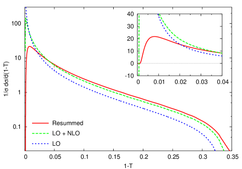
Figure 1: Comparison of the fixed-order (LO, NLO) and resummed (NLL) predictions for the thrust distribution in $e^{+}e^{-}$ at $Q=M_{Z}$. The resummed distribution has been matched ($\ln R$ scheme, see below) so as to include the full LO and NLO contributions. The inset differs from the main plot only in the scales.

To illustrate the impact of resummations we show in figure 1 the LO, NLO and resummed results for the thrust distribution. Not only is the divergence in the LO distribution clearly visible, but one also observes a marked difference in the qualitative behaviour of the LO and NLO results, both of which show large differences relative to the NLL resummed prediction at small $1-T$.

For the practical use of resummed results an important step is that of matching with the fixed-order prediction. At the simplest level one may think of matching as simply adding the fixed-order and resummed predictions while subtracting out the doubly counted (logarithmic) terms. Such a procedure is however too naive in that the fixed-order contribution generally contains terms that are subleading with respect to the terms included in the resummation, but which still diverge. For example when matching NLL and NLO calculations, one finds that the NLO result has a term $\sim R_{21}\alpha_{s}^{2}L$, which in the distribution diverges as $\alpha_{s}^{2}/v$. This is unphysical and the matching procedure must be sufficiently sophisticated so as to avoid this problem, and in fact it should nearly always ensure that the matched distribution goes to zero for $v\to 0$. Several procedures exist, such as $\ln R$ and $R$ matching [56] and multiplicative matching [68] and they differ from one-another only in terms that are NNLO and NNLL, i.e. formally beyond the state-of-the-art accuracy. We note the matching generally ensures that the resummation, in addition to being correct at NLL accuracy (our shorthand for NLL_lnR), is also correct at NNLL_R accuracy. Matching also involves certain other subtleties, for example the ‘modification of the logarithm’, whereby $\ln 1/v$ is replaced with $\ln(1+1/v-1/v_{\max})$, where $v_{\max}$ is the largest kinematically allowed value for the observable. This ensures that the logarithms go to zero at $v_{\max}$, rather than at some arbitrary point (usually $v=1$), which is necessary in order for the resulting matched distribution to vanish at $v_{\max}$.

4 Mean values, hadronisation corrections and comparisons to experiment

Much of the interest in event shapes stems from the wealth of data that is available, covering a large range of centre of mass energies ($e^{+}e^{-}$) or photon virtualities (DIS). The $e^{+}e^{-}$ data comes from the pre-LEP experiments [79], the four LEP experiments [80, 81, 82, 83, 84, 85] [86, 87, 88, 89] [90, 91, 92, 93, 94, 95, 96, 97, 98] [99, 100, 101, 102, 103] and SLD [104]. In addition, because many observables have been proposed only in the last ten or so years and owing to the particular interest (see below) in data at moderate centre of mass energies, the JADE data have been re-analysed [105, 106, 107, 108, 109]. Results in DIS come from both H1 [114, 115, 116] (mean values and distributions) and ZEUS [117] (means), [118] (means and distributions in rapidity gap events).

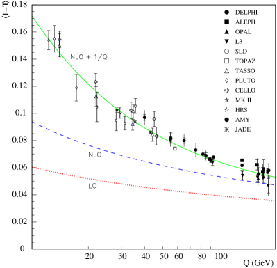
Figure 2: Left: data for the mean value of the $e^{+}e^{-}$ thrust, compared to LO, NLO and NLO+${\cal O}\left(\Lambda/Q\right)$; right: data for the Durham jet resolution $y_{23}$ compared to the NLO prediction (figure taken from [108]).

Let us start our discussion of the data by examining mean values (distributions are left until section 5). As we have already mentioned, one of the most appealing properties of event shapes, in terms of testing QCD, is the fact that they are calculable in perturbation theory and so provide a direct method for the extraction of $\alpha_{s}$ as well as testing other parameters of the theory such as the colour factors $C_{F}$ and $C_{A}$ by using a wealth of available experimental data. However one obstruction to the clean extraction of these fundamental parameters is the presence in many cases, of significant non-perturbative effects that typically fall as inverse powers $\propto 1/Q^{2p}$ of $Q$, the hard scale in the reaction (the centre-of–mass energy in $e^{+}e^{-}$ annihilation and the momentum transfer in DIS). The importance of such power corrections varies from observable to observable. For example, it can be seen from Fig. 2 (left) that the data for the mean value of the thrust variable need a significant component $\sim\Lambda/Q$ in addition to the LO and NLO fixed order perturbative estimates, in order to be described. On the other hand the comparison (right) for the mean value of the Durham jet resolution parameter $y_{23}$ with the NLO prediction alone is satisfactory, without the need for any substantial power correction term. The problem of non-perturbative corrections is so fundamental in event-shape studies that it is worthwhile giving a brief overview of the main approaches that are used.

4.1 Theoretical approaches to hadronisation corrections

No statement can be made with standard perturbative methods about the size of these power corrections and hence the earliest methods adopted to quantify them were phenomenological hadronisation models embedded in Monte Carlo event generators [10, 11, 12]. One of the main issues involved in using such hadronisation models is the existence of several adjustable parameters. This essentially means that a satisfactory description of data can be obtained by tuning the parameters, which does not allow much insight into the physical origin of such power behaved terms which are themselves of intrinsic theoretical interest (for a more detailed critique of hadronisation models see [119]).

However since the mid-nineties there have been developments that have had a significant impact on the theoretical understanding of power corrections. Perhaps the most popular method of estimating power corrections is based on the renormalon model. In this approach one examines high-order terms $\alpha_{s}^{n}$ of the perturbative series that are enhanced by coefficients $b^{n}n!$, where $b$ is the first coefficient of the $\beta$ function. The factorial divergence leads to an ambiguity in the sum of the series of order $(\Lambda/Q)^{2}p$, where the value of $p$ depends on the speed with which the high-order terms diverge. This approach has seen far more applications than can possibly be described here and for a full discussion and further references on renormalons the reader is referred to [13]. The most extensive phenomenological applications of renormalon based ideas have been in the estimation of power corrections for event-shape variables. The reason is that event shapes have much larger (and so experimentally more visible) power corrections (typically $\Lambda/Q$) than most other observables (typically $(\Lambda/Q)^{2}$ or smaller).

For event shape variables in $e^{+}e^{-}$ annihilation in the two-jet limit, renormalon-inspired (or related) studies of power corrections have been carried out in refs. [120, 121, 122, 123, 124, 125, 126, 127, 128, 129, 130, 64, 131, 132, 133, 134, 135, 136, 137, 28, 138, 70, 29, 139, 71, 140, 141, 142, 143]. For the $1+1$ jet limit of DIS, results on power corrections based on the renormalon approach can be found in [144, 145]. Studies in the $3$-jet limit have been given in [32, 34, 36, 18, 66, 146].

4.1.1 Dokshitzer-Webber approach.

The approach that has been most commonly used in comparing theoretical predictions with experimental data is that initiated by Dokshitzer and Webber [127, 128, 147, 129, 130, 64, 133, 134, 135, 136, 137, 144, 145]. Here the full result for the mean value, $\langle v\rangle$, is given by

$$\langle v\rangle=\langle v\rangle_{\mathrm{PT}}+C_{V}{\cal P}_{p}\,,$$ (22)

where $\langle v\rangle_{\mathrm{PT}}$ is the perturbative prediction for the mean value. The hadronisation correction is included through the term $C_{V}{\cal P}_{p}$, where $p$ is related to the speed of divergence of the renormalon series (as discussed above), $C_{V}$ is an observable-dependent (calculable) coefficient and ${\cal P}_{p}$ is a non-perturbative factor, scaling as $(\Lambda/Q)^{2p}$ which is hypothesised to be common across a whole class of observables with the same value of $p$ (strictly speaking the full story is a little more complicated, see e.g. [129]). Most event shapes have $p=1/2$, implying a leading power correction scaling as $\Lambda/Q$, essentially a consequence of the observables’ linearity on soft momenta. For these observables with $p=1/2$ the form for ${\cal P}\equiv{\cal P}_{1/2}$ that has become standard is [128, 134],

$${\cal P}\>\equiv\>\frac{4C_{F}}{\pi^{2}}{\cal M}\frac{\mu_{I}}{Q}\left\{\alpha_{0}(\mu_{I})-\alpha_{s}(\mu_{R})-\beta_{0}\frac{\alpha_{s}^{2}}{2\pi}\left(\ln\frac{\mu_{R}}{\mu_{I}}+\frac{K}{\beta_{0}}+1\right)\right\}\>,$$ (23)

where $\alpha_{s}\equiv\alpha_{\overline{\mbox{\scriptsize MS}}}(\mu_{R})$, $\beta_{0}=\frac{11}{3}C_{A}-\frac{2}{3}n_{f}$ and $K=C_{A}(67/18-\pi^{2}/6)-5n_{f}/9$. In eq. (23) an arbitrary infrared matching scale $\mu_{I}$ has been introduced, intended to separate the perturbative and non-perturbative regions. It is usually taken to be $2$ GeV (and for systematic error estimates it is varied between $1$ and $3$ GeV). The only truly non-perturbative ingredient in eq. (23) is $\alpha_{0}(\mu_{I})$, which can be interpreted as the average value of an infrared finite strong coupling for scales below $\mu_{I}$ (such a concept was first applied phenomenologically in [148]). Though one could imagine estimating it from lattice studies of the coupling (such as [149]), one should keep in mind that the coupling in the infrared is not a uniquely defined quantity. In practice the phenomenological test of the renormalon approach will be that $\alpha_{0}$ has a consistent value across all observables (in the $p=1/2$ class).

The terms with negative sign in the parenthesis in eq. (23) are a consequence of merging standard NLO perturbative results, which include the small spurious contributions from the infrared region (scales up to $\mu_{I}$), with the non-perturbative power correction that accounts correctly for scales from zero to $\mu_{I}$. Carrying out the subtraction of the perturbative terms that arise from the infrared region, below $\mu_{I}$, amounts to inclusion of the negative sign terms in parenthesis above. Note that this subtraction procedure must be carried out to the level of accuracy of the corresponding perturbative estimate. In other words if a perturbative estimate becomes available at $\mathcal{O}\left({\alpha_{s}^{3}}\right)$ then an additional subtraction term proportional to $\alpha_{s}^{3}$ is required. With the subtraction procedure carried out to $\mathcal{O}(\alpha_{s}^{2})$, as above, one expects a residual $\mu_{I}$ dependence $\sim\mathcal{O}\left({\alpha_{s}}^{3}(\mu_{I})\right)$. The scale $\mu_{R}$ is the renormalisation scale, which should be taken of the same order as the hard scale $Q$.

The ‘Milan factor’, ${\cal M}$ in eq. (23), is [133, 134, 136, 137, 145]

$${\cal M}=\frac{3}{64}\frac{(128\pi(1+\ln 2)-35\pi^{2})C_{A}-10\pi^{2}T_{R}n_{f})}{11C_{A}-4T_{R}n_{f}}\simeq 1.49\,,$$ (24)

where the numerical result is given for $n_{f}=3$, since only light flavours will be active at the relevant (low) scales. It accounts for the fact that the usual, ‘naive’, calculation for $C_{V}$ is carried out on the basis of a decaying virtual gluon (i.e. cutting a bubble in the chain of vacuum polarisation insertions that lead to the running of the coupling), but without fully accounting for the non-inclusiveness of that decay when dealing with the observable. It was pointed out in [150] that this is inconsistent and full (two-loop) calculations revealed [133, 134, 145] that if the ‘naive’ $C_{V}$ coefficient is calculated in an appropriate scheme, then the factor ${\cal M}$ comes out to be universal. As discussed in [134] this is essentially a consequence of the fact that regardless of whether one accounts for the virtual gluon decay, the distribution of ‘non-perturbative’ transverse momentum is independent of rapidity (the ‘tube-model’ of [151, 9], based essentially on boost invariance).

While the factor ${\cal M}$ corrects the $C_{V}$ at two-loop level, the question of even higher order corrections is still open, although one can argue that such effects will be suppressed by a factor $\sim\alpha_{0}(\mu_{I})/\pi$ relative to the leading power correction. This argument relies on the hope that the strong coupling remains moderate even in the infrared region.

$V$	$\tau$	$\rho$	$\rho_{h}$	$C$	$B_{T}$	$B_{W}$
$C_{V}$	$2$	$1$	$1$	$3\pi$	$\frac{\pi}{2\sqrt{C_{F}\alpha_{s}}}-\frac{\beta_{0}}{6C_{F}}+\bar{\eta}_{0}$	$\frac{\pi}{4\sqrt{2C_{F}\alpha_{s}}}-\frac{\beta_{0}}{24C_{F}}+\frac{\bar{\eta}_{0}}{2}$

Table 1: coefficients of $1/Q$ power corrections for $e^{+}e^{-}$ event shapes; $\bar{\eta}_{0}\simeq 0.136$.

$V$	$\tau_{tE}$	$\tau_{zE}$	$\rho_{E}$	$C_{E}$	$B_{tE}$	$B_{zE}$
$C_{V}$	$2$	$2$	$1$	$3\pi$	$\frac{\pi}{2\sqrt{C_{F}\alpha_{s}}}-\frac{\beta_{0}}{6C_{F}}+\bar{\eta}_{0}$	$\frac{\pi}{2\sqrt{2C_{F}\alpha_{s}}}-\frac{\beta_{0}}{12C_{F}}+$ $+\frac{\pi}{2C_{F}\alpha_{s}}\frac{d\ln q}{d\ln Q^{2}}+\bar{\eta}_{0}$

Table 2: coefficients of $1/Q$ power corrections for DIS event shapes; notation as in table 1 and additionally $q(x,Q^{2})=\sum_{j}e_{j}^{2}(q_{j}(x,Q^{2})+\bar{q}_{j}(x,Q^{2}))$, with the sum being over quark flavours.

Tables 1 and 2 display the values of the $C_{V}$ coefficients obtained in the 2-jet $e^{+}e^{-}$ and and $1+1$-jet DIS cases respectively. Note the different behaviour, proportional to $1/\sqrt{\alpha_{s}}$, that arises in the case of the jet broadenings in both processes, a consequence of the fact that the broadening is more sensitive to recoil induced by perturbative radiation [135]. The improved theoretical understanding that led to this prediction was strongly stimulated by experimental analysis [152] of features of earlier predictions [147, 134] that were inconsistent with the data. Since the origin of the $1/\sqrt{\alpha_{s}}$ enhancement is a perturbative, non-perturbative interplay best explained with reference to the power correction for the distribution, we delay its discussion to section 5.2.

Another consequence of this interplay of the broadening power correction with perturbative radiation is the fact that the DIS broadening $B_{zE}$ has a Bjorken $x$ dependent term corresponding to DGLAP evolution of the parton densities, as indicated by the term proportional to $d\ln q(x)/d\ln Q^{2}$ [68], where $q(x)$ denotes a parton density function. The coefficients for the other DIS variables are $x$ independent since in those cases the power correction arises from soft emission alone.

We also mention the result for the power correction to another interesting variable, the energy-energy correlation (EEC), in the back-to-back region. Like the broadening this variable exhibits the impact of perturbative-non–perturbative interplay. The results are fractional power corrections that vary as $1/Q^{0.37}$ (for the quark-gluon correlation) and $1/Q^{0.74}$ for the hard quark-antiquark correlation [64], instead of $1/Q$ and $\ln Q^{2}/Q^{2}$ contributions respectively, that would be obtained by considering NP emission without the presence of harder perturbative emissions.

Observables for which the power corrections have yet to be understood include the jet resolution parameters. Renormalon based predictions were given in [147] suggesting a $\Lambda/Q$ correction for $\langle y_{23}^{\mathrm{JADE}}\rangle$ and $(\Lambda/Q)^{2}$ for $\langle y_{23}^{\mathrm{Durham}}\rangle$. However it seems that in both cases there could be significant perturbative non-perturbative interplay which will complicate the picture. Nevertheless, as we have seen in fig. 2 (right) any correction to $\langle y_{23}^{\mathrm{Durham}}\rangle$ is certainly small compared to that for other observables.

A general point to be kept in mind is that the universality of $\alpha_{0}$ can be broken by contributions of order $\Lambda^{2}/m_{h}Q\sim\Lambda/Q$, where $m_{h}$ is the mass scale for hadrons [28]. Whether this happens or not depends on the hadron mass scheme in which the observable is defined (cf. section 2). Most observables are implicitly in the $p$-scheme, which generally involves a small negative breaking of universality (which is almost observable-independent, so that an illusion of universality will persist). The jet masses are an exception and in their usual definitions they have a significant (positive) universality breaking component. The $E$-scheme is free of universality breaking terms, as is the decay scheme (since hadron masses are zero). We also note that the power correction associated with hadron mass effects is enhanced by an anomalous dimension, $(\ln Q)^{A}$ with $A=4C_{A}/\beta_{0}\simeq 1.6$. The normal ‘renormalon’ power correction would also be expected to have an anomalous dimension, but it has yet to be calculated.

4.1.2 Higher moments of two-jet observables.

As well as studies of mean values (first moments) of observables there has also been work on higher-moments, $\langle v^{m}\rangle$ with $m>1$. Simple renormalon-inspired arguments suggest that the $m^{\mathrm{th}}$ moments of event shapes should have as their leading power correction at most a $(\Lambda/Q)^{m}$ contribution (essentially since $v^{m}$ vanishes at $(k_{t}/Q)^{m}$ for small $k_{t}$). However as was pointed out by Webber [153], the fact (to be discussed in section 5.2) that the $\Lambda/Q$ power correction essentially corresponds to a shift of the distribution (for $T$, $C$ and $\rho_{H}$, but not for the broadenings), means that to a first approximation we will have

$$\langle v^{m}\rangle=\langle v^{m}\rangle_{\mathrm{PT}}+m\,\langle v^{m-1}\rangle_{\mathrm{PT}}\,C_{V}{\cal P}+\ldots\,.$$ (25)

Given that $\langle v^{m-1}\rangle_{\mathrm{PT}}$ is of order $\alpha_{s}$, all higher moments of event shapes will receive power corrections of order $\alpha_{s}\Lambda/Q$, which is parametrically larger than $(\Lambda/Q)^{m}$. Strictly speaking it is not possible to guarantee the coefficient of $\alpha_{s}\Lambda/Q$ given in eq. (25), since the shift approximation on which it is based holds only in the $2$-jet region, whereas the dominant contribution to the relevant integral comes from the $3$-jet region. For the $C$-parameter an alternative coefficient for the $\alpha_{s}\Lambda/Q$ power correction has been proposed in [124], however since it also is not based on a full calculation of the power correction in the three-jet region (which does not yet exist), it is subject to precisely the same reservations as eq. (25).

We note also an interesting result by Gardi [139] regarding the exact renormalon analysis of $\langle(1-T)^{2}\rangle$. While it is clear that the physical answer $\alpha_{s}\Lambda/Q$ will not appear in a leading renormalon analysis (the extra factor of $\alpha_{s}$ means that it is associated with a subleading renormalon) the calculation [139] has the surprising result that the leading renormalon contribution is not $(\Lambda/Q)^{2}$ as naively expected but rather $(\Lambda/Q)^{3}$.

4.1.3 Power corrections to three-jet observables.

Considerable progress has been made in recent years in the calculation of power corrections for three-jet observables (those that vanish in the two and the three-jet limits). In the three-jet limit, there exist explicit results for the thrust minor [18] and the $D$-parameter [66] in $e^{+}e^{-}\to 3\;\mathrm{jets}$, the out of plane momentum in Drell-Yan plus jet [36] and in $2+1$-jet DIS [32], as well as azimuthal correlations in DIS [34]. Except for the $D$-parameter, all these calculations involve perturbative, non-perturbative interplay in a manner similar to that of the broadenings and back-to-back EEC. The explicit forms for the results are rather complicated and so we refer the reader to the original publications.

Simpler (though numerical) results have been obtained [146] in the case of the $D$-parameter (confirmed also by [66, 154]) integrated over all 3-jet configurations, where one finds

$$C_{D}\,\simeq\,\left(118.0+34.7\frac{C_{A}}{C_{F}}\right)\frac{\alpha_{s}(\mu_{R})}{2\pi}\,\simeq\,196.0\frac{\alpha_{s}(\mu_{R})}{2\pi}\,.$$ (26)

The power of $\alpha_{s}$ comes from the matrix-element weighting of the $3$-jet configurations and the fact that the $D$-parameter vanishes in the $2$-jet limit.

A final $3$-jet result of interest [146] is that for the $C$-parameter just above the Sudakov shoulder, at $C=3/4$. This is the only case where a proper calculation exists for the power correction to a two-jet observable in the three jet limit:

$$C_{C@\frac{3}{4}}\,\simeq\,2.110\left(1+\frac{C_{A}}{2C_{F}}\right)\,\simeq\,4.484\,.$$ (27)

This is slightly less than half the correction that appears in the two-jet limit ($C_{C}=3\pi$).

A point that emerges clearly from eqs. (26) and (27), but that is relevant for all $3$-jet studies is that the power correction acquires a dependence on $C_{A}$, i.e. there is sensitivity to hadronisation from a gluon. In situations where one selects only three-jet events there is additionally non trivial dependence on the geometry, due to the coherence between the three jets. Comparisons to data for such observables would therefore allow a powerful test of the renormalon-inspired picture. In particular, other models, such as the flux tube model [151, 9] (based essentially on boost invariance along the $q\bar{q}$ axis), which in the $2$-jet limit give the same predictions as renormalon-inspired approaches, cannot as naturally be extended to the $3$-jet case.

4.2 Fits to data

One of the most widespread ways of testing the Dokshitzer-Webber approach to hadronisation is to carry out simultaneous fits to the mean value data for $\alpha_{s}$ and $\alpha_{0}$. Figure 2, where the term labelled $1/Q$ is actually of the form $C_{V}{\cal P}$, shows the good agreement that is obtained with the thrust data. The quality of agreement is similar for other observables (see for example fig. 11 of [89]).

The true test of the approach however lies in a verification of the universality hypothesis, namely that $\alpha_{0}$ is the same for all observables and processes. While there are strong general reasons for expecting universality within $e^{+}e^{-}$ (boost invariance and the flux-tube model), universality across difference processes is less trivial — for example one could imagine DIS hadronisation being modified by interactions between outgoing low-momentum gluons (or hadrons) and the ‘cloud’ of partons that make up the proton remnant (present even for a fast-moving proton, since the longitudinal size of the cloud is always of order $1/\Lambda$).

Figure 3 shows $1$-$\sigma$ contours for fits of $\alpha_{s}$ and $\alpha_{0}$ in $e^{+}e^{-}$ [28] (left, all experiments combined) and DIS (right, H1 [115, 116] and ZEUS [117] merged into one plot). Aside from the different scales used, some care is required in reading the figures because of different treatments of the errors in the different plots. For example H1 include experimental systematic errors whereas ZEUS do not. In the $e^{+}e^{-}$ fit, the systematics are included but treated as uncorrelated, which may underestimate the final error. In neither figure are theoretical uncertainties included: over the available range of $e^{+}e^{-}$ energies, renormalisation scale dependence gives an uncertainty of about $\pm 0.005$ on $\alpha_{s}$, while a ‘canonical’ variation of the Milan factor $\cal M$ by $\pm 20\%$ (to allow for higher-order terms) leads to an uncertainty of ${}^{+0.09}_{-0.06}$ on $\alpha_{0}$ [108]. In DIS the corresponding uncertainties are larger for $\alpha_{s}$ ($\pm 0.09)$, essentially because the fits are dominated by lower $Q$ values, and they vary substantially for $\alpha_{0}$ (larger for photon-axis observables, smaller for the others). Also to be kept in mind is that the DIS figure includes the jet mass, $\rho_{E}$ in the default scheme, and in $e^{+}e^{-}$ the origins of the arrows indicate the default-scheme results for $\rho$ and $\rho_{H}$. Since the default scheme for jet masses breaks universality (cf. section 4.1.1) these results should not be compared directly to those for other observables.

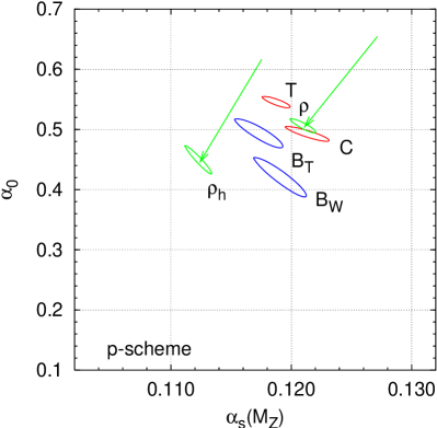
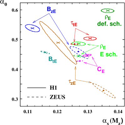
Figure 3: Left: $\alpha_{s}$, $\alpha_{0}$ fit to $e^{+}e^{-}$ data on mean values of event shapes, with the jet masses converted to the $p$-scheme (the arrow indicates the change in going from default to $p$-scheme) [28]. Right: fits to DIS mean event-shape data by H1 [115, 116] and ZEUS [117] (curves taken from figures in [116, 117]). Contours indicate 1-$\sigma$ uncertainties (statistical and experimental systematic, except for the ZEUS results which are just statistical).

Taking into account the uncertainties, which are not necessarily correlated from one observable to another, fig. 3 indicates remarkable success for the renormalon-inspired picture. The results are in general consistent with a universal value for $\alpha_{0}$ in the range $0.45$ to $0.50$. Furthermore the $e^{+}e^{-}$ results for $\alpha_{s}$ are in good agreement with the world average. On the other hand the DIS results for $\alpha_{s}$ seem to be somewhat larger than the world average. The discrepancy is (just) within the theoretical systematic errors, however it remains a little disturbing and one wonders whether it could be indicative of large higher-order corrections, or some other problem (known issues include the fact that the low-$Q$ data can bias the fits, for example because of heavy-quark effects and $\Lambda^{2}/Q^{2}$ corrections; and also at high-$Q$ there is $\gamma/Z$ interference which is not usually accounted for in the fixed-order calculations). There is potentially also some worry about the $\tau_{zE}$ result which has an anomalously low $\alpha_{0}$ and large $\alpha_{s}$ (and additionally shows unexpectedly substantial $x$ dependence [117]).

Another point relates to the default scheme jet masses — though the universality-breaking effects should be purely non-perturbative, they have an effect also on the fit results for $\alpha_{s}$. This is a consequence of the anomalous dimension that accompanies $\Lambda/Q$ hadron mass effects. Similar variations of $\alpha_{s}$ are seen when varying the set of particles that are considered stable [28].

Though as discussed above some issues remain, they should not however be seen as detracting significantly from the overall success of the approach and the general consistency between $e^{+}e^{-}$ and DIS. We also note that the first moment of the coupling as extracted from studies of heavy-quark fragmentation [148, 156] is quite similar to the value found for event shapes.

There have also been experimental measurements of higher moments of event shapes, notably in [97]. The parameters $\alpha_{s}$ and $\alpha_{0}$ are fixed from fits to mean values and then inserted into eq. (25) to get a prediction for the second moments. For $\langle\rho_{H}^{2}\rangle$ this gives very good agreement with the data (though the fact that $\rho_{H}$ is in the default scheme perhaps complicates the situation), while $\langle(1-T)^{2}\rangle$ and $\langle C^{2}\rangle$ show a need for a substantial extra correction. In [97] this extra contribution is shown to be compatible with a $\Lambda^{2}/Q^{2}$ term, though it would be interesting to see if it is also compatible with a $\alpha_{s}{\cal P}$ term with a modified coefficient.

Currently (to our knowledge) no fits have been performed for three-jet event shapes, though we understand that such fits are in progress [157] for the mean value of the $D$-parameter. We look forward eagerly to the results. In the meantime it is possible to verify standard parameters for $\alpha_{s}$ and $\alpha_{0}$ against a single published point at $Q=M_{Z}$ [91, 85] and one finds reasonable agreement within the uncertainties.

4.3 Fits with alternative perturbative estimates.

Two other points of view that have also been used in analysing data on $e^{+}e^{-}$ event shapes are the approach of dressed gluons employed by Gardi and Grunberg [138] and the use of renormalisation group improved perturbation theory [158] as carried out by the DELPHI collaboration [89].

4.3.1 Gardi–Grunberg approach.

In the Gardi-Grunberg approach one uses the basic concept of renormalons (on which the DW model is also based), but one choses to treat the renormalon integral differently to the DW model. This renormalon integral is ill-defined due to the Landau singularity in the running coupling and instead of assuming an infrared finite coupling below some matching scale $\mu_{I}$ as was the case in the DW model, Gardi and Grunberg define the renormalon integral by its principal value (a discussion of the theoretical merits of different approaches has been give in [159]). In doing this they explicitly include higher order renormalon contributions in their perturbative result, rather than including them via power behaved corrections below scale $\mu_{I}$ that result from assuming an infrared finite coupling (though they do also compare to something similar, which they call a ‘cutoff’ approach). However since one is dealing with an ambiguous integral (a prescription other than a principal value one would give a result differing by an amount proportional to a power correction) one must still allow for a power correction term. Gardi and Grunberg studied the mean thrust in $e^{+}e^{-}$ annihilation and used the following form for fitting to the data :

$$\langle 1-T\rangle=\frac{C_{F}}{2}[R_{0}|_{\mathrm{PV}}+\delta_{\mathrm{NLO}}]+\frac{\lambda}{Q}$$ (28)

where the subscript PV denotes the principal value of the renormalon integral $R_{0}$ for the thrust (which includes the full LO contribution and parts of the higher-order contributions) and $\delta_{\mathrm{NLO}}$ is a piece that accounts for the difference between the true NLO coefficient for $1-T$ and the contribution included in $R_{0}$.

Figure 4: The mean value of the thrust distribution in $e^{+}e^{-}$ annihilation as a function of $Q$ with $\alpha_{s}^{\hbox{$\overline{\hbox{\tiny MS}}\,$}}({\rm M_{Z}})=0.110$. The upper (dashed) line corresponds to the principal value result which then is fitted to the data adding a $1/Q$ term. Figure taken from Ref. [160].

The best fit values obtained for $\alpha_{s}^{\hbox{$\overline{\hbox{\tiny MS}}$}}({\rm M_{Z}})$ and $\lambda$ are respectively $0.110\pm 0.006$ and $0.62\pm 0.11$. We note that $\lambda\simeq 0.6$ in this approach corresponds to a smaller power correction than is required in the DW model. This is probably a consequence of the inclusion of pieces of higher perturbative orders via a principal value prescription, although it leads to a somewhat small value (compared to the world average) of the coupling at scale $M_{z}$.

4.3.2 Renormalisation group improved approach.

Next we turn to the renormalisation group improved (RGI) perturbative estimates [158, 161, 162] that have also been used to compare with event shape data for the mean value of different event shapes in $e^{+}e^{-}$ annihilation. The basic idea behind this approach is to consider the dependence of the observable on the scale $Q$, which can be expressed using renormalisation group invariance as

$$Q\frac{dR}{dQ}=-bR^{2}(1+\rho_{1}R+\rho_{2}R^{2}+\cdots)=b\rho(R)$$ (29)

where in the above formula $b=\beta_{0}/2$, $R=2\langle f\rangle/A$, with $\langle f\rangle$ being the mean value of a given event shape and $A$ being the coefficient of $\alpha_{s}/2\pi$ in its perturbative expansion.

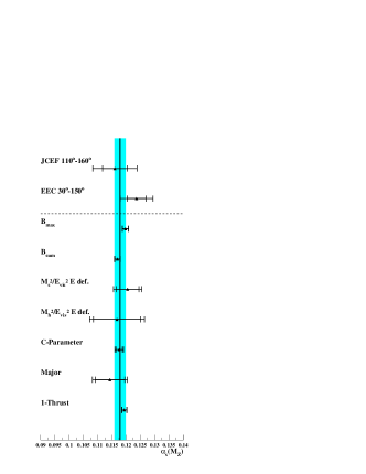
Figure 5: Results for $\alpha_{s}(M_{z})$ from comparisons to $e^{+}e^{-}$ event-shape data using the RGI approach. The band shows the mean value of $\alpha_{s}$ and uncertainty, as obtained from the observables below the dashed line. Figure taken from Ref. [89].

Thus the first term in the perturbative expansion of $R$ is simply $\alpha_{s}/\pi$. The $\rho_{i}$ are renormalisation scheme independent quantities. In particular the quantity $\rho_{1}=\beta_{1}/(2\beta_{0})$ is simply the ratio of the first two coefficients of the QCD $\beta$ function while $\rho_{2}$ additionally depends on the first three (up to NNLO) perturbative coefficients in the expansion of $\langle f\rangle$. Current studies using this method are therefore restricted to an NLO analysis involving $\rho_{1}$ alone. With this simplification, the solution of eq. (29) simply corresponds to the introduction of an observable-specific renormalisation scheme and associated scale parameter $\Lambda_{R}$ which is such that it sets the NLO perturbative term to be zero (and neglects higher perturbative orders). Its relation to the standard $\Lambda_{\overline{\mathrm{MS}}}$ is easily obtained:

$$\frac{\Lambda_{R}}{\Lambda_{\overline{\mathrm{MS}}}}=e^{\frac{r_{1}}{b}}\left(\frac{2c_{1}}{b}\right)^{-\frac{c_{1}}{b}},$$ (30)

where $c_{1}=\rho_{1}$ and $r_{1}=B/2A$, with $B$ being the NLO coefficient in the $\overline{\mathrm{MS}}$ expansion for the observable. The terms in the bracket account for different definitions of the coupling in terms of $\Lambda$ as used in the $R$ and $\overline{\mathrm{MS}}$ schemes.

In the specific case of fits to $e^{+}e^{-}$ event shape mean values, the above approach has met with a considerable success [89]. In particular the introduction of $\Lambda_{R}$ seems to remove any need for a significant power correction. The DELPHI collaboration [89] have performed a combined fit of the parameter $\Lambda_{R}$ and a parameter $K_{0}$ that quantifies the power correction [161, 89]. The value of $K_{0}$ was found to be consistent with zero in most cases and rather small in all cases which indicates that there is no real need for a power behaved correction once the perturbative expansion is fixed through the RGI technique. The agreement between $\alpha_{s}$ values extracted from different observables is impressive (see figure 5) with a spread that is only about half as large as that obtained using the standard perturbative result supplemented by a power correction term, using the DW initiated model.

While it is clear that the size of the power correction piece inevitably depends on how one choses to define the perturbative expansion (in fact all the methods discussed thus far, including the DW model and the Gardi-Grunberg approach, account for this effect), it is nevertheless very interesting that for several different observables, with significantly different perturbative coefficients, one observes after the introduction of RGI, hardly any need for a power correction term. Certainly it is not clear on the basis of any physical arguments, why the genuine non-perturbative power correction should be vanishingly small and that a perturbative result defined in a certain way should lead to a complete description of the data. The clarification of this issue is still awaited and the above findings are worth further attention and study.

A final point to be kept in mind about the RGI approach in the above form, is that it is valid only for inclusive observables that depend on just a single relevant scale parameter $Q$. This makes its applicability somewhat limited and for instance it is not currently clear how to extend the procedure so as to allow a meaningful study of event shape distributions in $e^{+}e^{-}$ annihilation or DIS event shape mean values and distributions (which involve additional scales).

5 Distributions

So far our discussion of comparisons between theory and experiment has been limited to a study of mean values of the event shapes. As we have seen, there is some ambiguity in the interpretation of these comparisons, with a range of different approaches being able to fit the same data. This is in many respects an unavoidable limitation of studies of mean values, since the principal characteristic of the different models that is being tested is their $Q$-dependence, which can also be influenced by a range of (neglected) higher-order contributions. In contrast, the full distributions of event shapes contain considerably more information and therefore have the potential to be more discriminatory.

In section 3 we discussed the perturbative calculation of distributions. As for mean values though, the comparison to data is complicated by the need for non-perturbative corrections. These corrections however involve many more degrees of freedom than for mean values, and there are a variety of ways of including them. Accordingly we separate our discussion into two parts: in section 5.1 we shall consider studies in which hadronisation corrections are taken from Monte Carlo event generators, and where the main object of study is the perturbative distribution, with for example fits of the strong coupling. In section 5.2 we shall then consider studies which involve analytical models for the non-perturbative corrections, and where it is as much the non-perturbative models, as the perturbative calculations that are under study.

5.1 Perturbative studies with Monte Carlo hadronisation

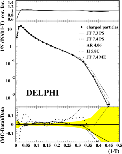
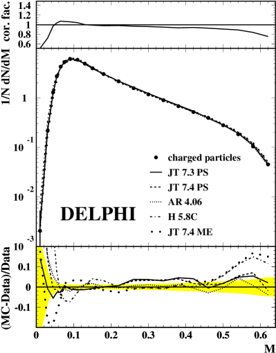
Figure 6: Event shape distributions at $M_{Z}$ compared to a variety of event generators [10, 11, 12]. The shaded band in the lower plot indicates the experimental statistical and systematic errors added in quadrature. Figure taken from [163].

5.1.1 Use of Monte Carlo event generators.

Before considering the purely perturbative studies mentioned above, let us recall that one major use of event shape distributions has been in the testing and tuning [163, 164, 165] of Monte Carlo event generators such as Herwig [10], Jetset/Pythia [11] and Ariadne [12]. Figure 6 shows comparisons for two event shapes, the thrust and thrust major, and the agreement is remarkable testimony to the ability of the event generators to reproduce the data.

The use of event generators to probe the details of QCD is unfortunately rather difficult, essentially because they contain a number of parameters affecting both the non-perturbative modelling and in some cases the treatment of the perturbative shower. Furthermore though considerable progress is being made in matching to fixed order calculations (see for example [166]), event generators are in general able to guarantee neither the NLL accuracy nor the NLO accuracy of full matched NLL-NLO resummed calculations.

Nevertheless, the good agreement of the event generators with the data suggests that the bulk of the dynamics is correct and in particular that a good model for the hadronisation corrections can be had by comparing parton and hadron ‘levels’ of the generator. There has been a very widespread use of event generators in this way to complement the NLL+NLO perturbative calculations.

Such a method has both advantages and drawbacks and it is worth devoting some space to them here. On one hand, the parton level of an event generator is not a theoretically well-defined concept — it is regularised with some effective parton mass or transverse momentum cutoff, which already embodies some amount of non-perturbative correction. In contrast the NLO+NLL partonic prediction integrates down to zero momenta without any form (or need) of regularisation. This too implies some amount of non-perturbative contribution, but of a rather different nature from that included via a cutoff. The resulting difference between the event-generator and the purely perturbative NLO+NLL parton levels means that the ‘hadronisation’ that must be applied to correct them to hadron level is different in the two cases.

There are nevertheless reasons why event-generators are still used for determining the hadronisation corrections. The simplest is perhaps that they give a very good description of the data (cf. fig. 6), which suggests that they make a reasonable job of approximating the underlying dynamics. Furthermore the good description is obtained with a single set of parameters for all event shapes, whereas as we shall see, other approaches with a single (common) parameter are currently able to give equally good descriptions only for a limited number of event shapes at a time. Additionally, the objection that the Monte Carlo parton level is ill-defined can, partially, be addressed by including a systematic error on the hadronisation: it is possible for example to change the internal cutoff on the Monte Carlo parton shower and at the same time retune the hadronisation parameters in such a way that the Monte Carlo description of the hadron-level data remains reasonable. In this way one allows for the fact that the connection between Monte Carlo and NLL+NLO ‘parton-levels’ is not understood. This is the procedure that has been used for example in [104], and the results are illustrated in figure 7 as a hadronisation correction factor $C_{H}$ with an uncertainty corresponding to the shaded band.

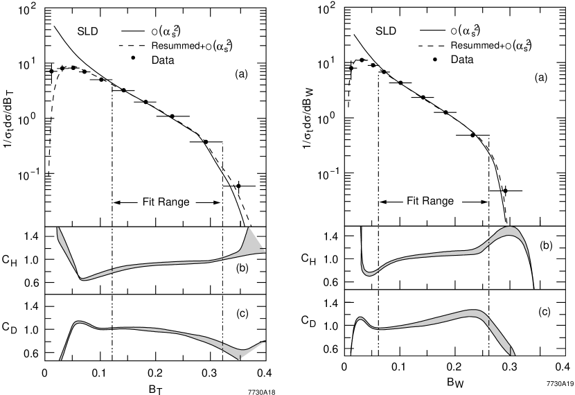
Figure 7: SLD data for the total and wide-jet broadenings, transformed to ‘parton’ level using a multiplicative bin-by-bin factor ($C_{H}$, with uncertainties, as discussed in the text) obtained from the ratio of Jetset parton to hadron-level distributions. It is compared to NLO and NLL+NLO predictions. Also shown is the detector to hadron-level correction factor $C_{D}$. Figure taken from [104].

Two further points are to be made regarding Monte Carlo hadronisation corrections. Firstly, as is starting now to be well known, it is strongly recommended not to correct the data to parton-level, but rather to correct the theoretical perturbative prediction to hadron level. This is because the correction to parton level entails the addition of extra assumptions, which a few years later may be very difficult to deconvolve from the parton-level ‘data’. It is straightforward on the other hand to apply a new hadronisation model to a perturbative calculation.

Secondly it is best not to treat the hadronisation correction as a simple multiplicative factor. To understand why, one should look again at figure 7 (which, dating from several years ago, corrects data to parton level). The multiplicative factor $C_{H}$ (parton$/$hadron) varies very rapidly close to the peak of the distribution and goes from above $1$ to below $1$. This is because the distribution itself varies very rapidly in this region and the effect of hadronisation is (to a first approximation, see below) to shift the peak to larger values of the observable. But a multiplicative factor, rather than shifting the peak, suppresses it in one place and recreates it (from non-peak-like structure) in another. Instead of applying a multiplicative correction, the best way to include a Monte Carlo hadronisation correction is to determine a transfer matrix $M_{ij}$ which describes the fraction of events in bin $j$ at parton level that end up in in bin $i$ at hadron level. Then for a binned perturbative distribution $P_{i}$, the binned hadronised distribution $H_{i}$ is obtained by matrix multiplication, $H_{i}=M_{ij}P_{i}$. This has been used for example in [83, 85].

5.1.2 NLL+NLO perturbative studies.

Having considered the basis and methods for including hadronisation corrections from event generators, let us now examine some of the perturbative studies made possible by this approach. The majority of them use NLL+NLO perturbative calculations to fit for the strong coupling (as discussed below some, e.g. [88], just use NLO results, which exist for a wider range of observables) and such fits can be said to be one of the principal results from event-shape studies. In general there is rather good agreement between the data and the resummed predictions (cf. fig. 7).

Figure 8: Values for $\alpha_{s}$ obtained by fitting NLL+NLO event-shape distributions to L3 data at a range of centre of mass energies (figure taken from [98]). Only experimental uncertainties are shown.

An example of such a study is given in figure 8, which shows results for fits of $\alpha_{s}$ to L3 data at a range of energies (including points below $M_{Z}$ from radiative events which, as discussed earlier, are to be taken with some caution). One important result from such studies is an overall value for $\alpha_{s}$, which in this case is $\alpha_{s}(M_{Z})=0.1227\pm 0.0012\pm 0.0058$ [98], where the first error is experimental and the second is theoretical. Similar results have been given by other collaborations, e.g. $\alpha_{s}(M_{Z})=0.1195\pm 0.0008\pm 0.0034$ from ALEPH [84]. There is also good evidence for the evolution of the coupling, though leaving out the potentially doubtful radiative points leaves the situation somewhat less clearcut, due to the limited statistics at high energies (another resummed study which gives good evidence for the running of the coupling uses JADE and OPAL data [107], however it is limited to jet rates).

These and similar results from the other LEP collaborations and JADE highlight two important points. Firstly at higher energies there is a need to combine results from all the LEP experiments in order to reduce the statistical errors and so improve the evidence for the running of the coupling in the region above $Q=M_{Z}$. Work in this direction is currently in progress [168]. So far only preliminary results are available [169], and as well as improving the picture of the high-energy running of the coupling, they suggest a slightly smaller value of $\alpha_{s}$ than that quoted above, more in accord with world averages [170, 171].

Secondly, in the overall result for $\alpha_{s}(M_{Z})$, by far the most important contribution to the error is that from theoretical uncertainties. However theoretical uncertainties are notoriously difficult to estimate, since they relate to unknown higher orders. Systematic investigations of the various sources of uncertainty have been carried out in [33, 172] and in particular [172] proposes a standard for the set of sources of uncertainty that ought to be considered, together with an approach for combining the different sources into a single overall uncertainty on $\alpha_{s}$. One of the main principles behind the method is that while one may have numerous estimates of sources of theoretical uncertainty, it is not advisable to combine them in quadrature, as one might be tempted to do, because this is likely to lead to a double-counting of uncertainties. Rather, one should examine the different sources of uncertainty across the whole range of the distribution and at each point, take the maximum of all sources to build up an uncertainty envelope or band, represented by the shaded area in figure 9 (shown relative to a reference prediction for a ‘standard’ theory). The overall uncertainty on the coupling (rather than the distribution) is given by the range of variation of $\alpha_{s}$ such that the prediction remains within the band. It is to be noted that this kind of approach is of relevance not just to event-shape studies but also quite generally to any resummed matched calculation, which is inherently subject to many sources of arbitrariness.

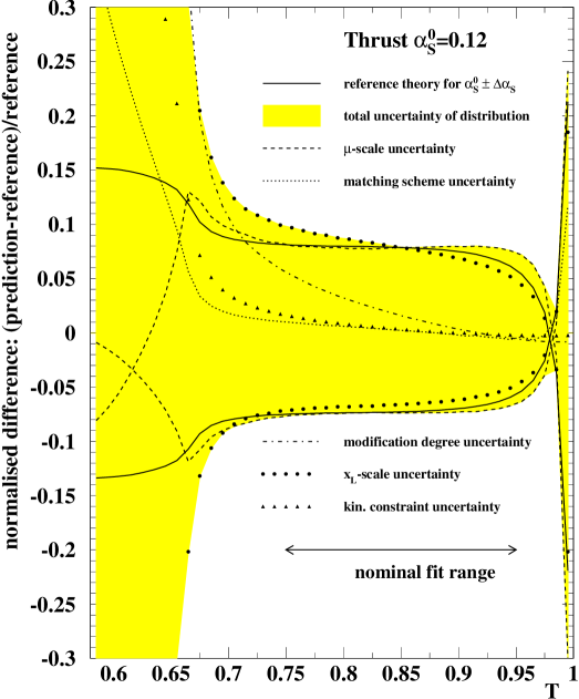
Figure 9: Theoretical uncertainties for the thrust. The shaded area represents the overall theoretical uncertainty on the distribution, determined as the maximum/minimum of all the dashed, dotted, etc. curves; the solid curves indicate the variation of $\alpha_{s}$ allowed such that the prediction stays within the uncertainty band.

5.1.3 Other perturbative studies.

One of the drawbacks of NLL+NLO studies is that the NLL resummed predictions exist for only a fraction of observables. Recently there has been an extensive study by the DELPHI collaboration [88] of 18 event-shape distributions compared to NLO calculations. Since in most cases NLO calculations with a renormalisation scale $\mu_{R}=Q$ tend to describe the data rather poorly, they have examined various options for estimating higher orders so as to improve the agreement. Their main approach involves a simultaneous fit of the coupling and the renormalisation scale, i.e. the renormalisation scale dependence is taken as a way of parameterising possible higher orders. In such a procedure the choice of fit-range for the observable is rather critical, since the true higher-orders may involve have quite a different structure from that parameterised by the $\mu_{R}$ dependence. The DELPHI analysis restricts the fit range to be that in which a good fit can be obtained. With these conditions they find relatively consistent values of $\alpha_{s}$ across their whole range of observables (finding a scatter of a few percent), with a relatively modest theoretical uncertainty, as estimated from the further variation of $\mu_{R}$ by a factor of $1/2$ to $2$ around the optimal scale. Their overall result from all observables treated in this way is $\alpha_{s}=0.1174\pm 0.0026$ (including both experimental and theoretical errors).

They also compare this approach to a range of other ways of ‘estimating’ higher orders. They find for example that some theoretically based methods for setting the scale (principle of minimal sensitivity [173], effective charge [174]) lead to scales that are quite correlated to the experimentally fitted ones, while another method (BLM [175]) is rather uncorrelated. They compare also to resummation approaches, though there is no equivalent renormalisation scale choice that can be made. Instead the comparison involves rather the quality of fit to the distribution and the final spread of final $\alpha_{s}$ values as a measure of neglected higher-order uncertainties. Not surprisingly, they find that while the NLL results work well in the two-jet region, in the three-jet region the combined NLL+NLO predictions fare not that much better than the pure ($\mu_{R}=Q$) NLO results. They go on to argue that NLL+NLO is somewhat disfavoured compared to NLO with an ‘optimal’ scale. This statement is however to be treated with some caution, since the fit range was chosen specifically so as to obtain a good fit for NLO with the ‘optimal’ scale — one could equally have chosen a fit range tuned to the NLL+NLO prediction and one wonders whether the NLO with optimal scale choice would then have fared so well. Regardless of this issue of fit range, it is interesting to note that over the set of observables which can be treated by both methods, the total spread in $\alpha_{s}$ values is quite similar, being $\pm 0.04$ in the case of NLO with optimal scale choice and $\pm 0.05$ for NLL+NLO. This is similar to the spread seen for fits to mean values with analytical hadronisation models (fig. 3), though the RGI fits of [89] have a somewhat smaller error.

The jet rates (especially the Durham and Cambridge algorithms and certain members of the JADE family) are among the few observables for which the pure NLO calculation gives a reasonable description of the distribution (cf. table 3 of [88]). One particularly interesting set of NLO studies makes use of the 3-jet rate as a function of $y_{cut}$ (this is just the integral of the distribution of $y_{23}$) in events with primary $b$-quarks as compared to light-quark events [176, 177, 178, 179, 180] (some of the analyses use other observables, such as the 4-jet rate or the thrust). Using NLO calculations which account for massive quarks [181, 182, 183] makes it possible, in such studies, to extract a value for the $b$ mass at a renormalisation scale of $M_{Z}$, giving first evidence of the (expected) running of the $b$-quark mass, since all the analyses find $M_{b}(M_{Z})$ in the range $2.6$ to $3.3$ GeV (with rather variable estimates of the theoretical error).

5.2 Studies with analytical hadronisation models

We have already seen, in section 4, that analytical models for hadronisation corrections, combined with normal perturbative predictions, can give a rather good description of mean values. There the inclusion of a non-perturbative (hadronisation) correction was a rather simple affair, eq. (22), since it was an additive procedure. In contrast the general relation between the full distribution $D_{V}(v)$ for an observable $V$ and the perturbatively calculated distribution $D_{\mathrm{PT},V}$ is more complicated,

$$D_{V}(v)=\int dx\,f_{V}(x,v,\alpha_{s}(Q),Q)\,D_{\mathrm{PT},V}\left(v-\frac{x}{Q}\right)\,,$$ (31)

where $f_{V}(x,v,\alpha_{s}(Q),Q)$ encodes all the non-perturbative information. Eq. (31) can be seen as a generalised convolution, where the shape of the convolution function depends on the value $v$ of the variable as well as the coupling and hard scale. Such a general form contains far more information however than can currently be predicted, or even conveniently parameterised. Accordingly analytical hadronisation approaches generally make a number of simplifying assumptions, intended to be valid for some restricted range of the observable.

5.2.1 Power correction shift.

The most radical simplification of eq. (31) that can be made is to replace $f_{V}(x,v,\alpha_{s}(Q),Q)$ with a $\delta$-function, $\delta(x-C_{V}\mathcal{P})$, leading to

$$D_{{\mathrm{NP}},V}(v)=D_{{\mathrm{PT},V}}(v-C_{V}\mathcal{P})\,,$$ (32)

This was proposed and investigated in [130], and the combination $C_{V}\mathcal{P}$ is the same that appears in the power correction for the mean value [128], discussed in section 4. Eq. (32) holds for observables with an $\alpha_{s}$ independent power correction in tables 1 and 2, in the region $\Lambda/Q\ll v\ll 1$, where the lower limit ensures that one can neglect the width of the convolution function $f_{V}$, while the upper limit is the restriction that one be in the Born limit (in which the $C_{V}$ were originally calculated). For certain 3-jet observables a similar picture holds, but with a shift that depends on the kinematics of the 3-jet configuration [18, 66].

For the broadenings, the situation is more complicated because the power correction is enhanced by the rapidity over which the quark and thrust axes can be considered to coincide, $\ln 1/\theta_{Tq}$, $\theta_{Tq}$ being the angle between thrust and quark axes — this angle is strongly correlated with the value of the broadening (determined by perturbative radiation) and accordingly the extent of the shift becomes $B$-dependent [135]. The simplest case is the $e^{+}e^{-}$ wide-jet broadening, for which one has

$$\Sigma_{\mathrm{NP},B_{W}}(v)=\Sigma_{\mathrm{PT},B_{W}}\left(v-\frac{D_{1}(v)\mathcal{P}}{2}\right),\qquad D_{1}(v)\sim\ln\frac{1}{v}\,,$$ (33)

where the shift is written for the integrated distribution $\Sigma_{\mathrm{NP},B_{W}}(v)$ in order to simplify the expressions. The $1/\sqrt{\alpha_{s}}$ enhancement for the power correction to the mean broadening (tables 1 and 2) comes about simply because the average value of $\ln\frac{1}{v}$, after integration over $v$ with the resummed distribution, is of order $1\sqrt{\alpha_{s}}$.

The full form for $D_{1}(v)$ and analogous results for the total $e^{+}e^{-}$ and DIS broadenings have been given in [135, 68], with results existing also for the thrust minor [18], and the DIS and Drell-Yan out-of plane momenta [32, 36]. Yet subtler instances of perturbative, non-perturbative interplay arise for observables like the EEC [64] and DIS azimuthal correlation [34], with the appearance of fractional powers of $Q$ in the power correction, as mentioned before.

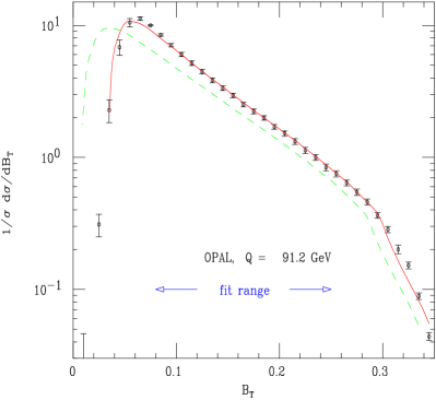
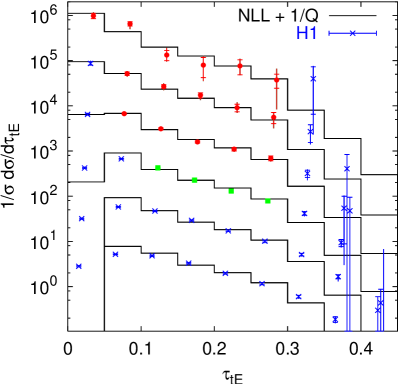
Figure 10: Left: Illustration of the $B_{T}$-dependent non-perturbative shift in the jet broadening distribution for $e^{+}e^{-}$ annihilation. The dashed curve is the perturbative prediction (NLL+NLO), while the solid curve includes a non-perturbative ($B$-dependent) shift. Figure taken from [135]. Right: NLL+NLO distribution with a $1/Q$ shift for $\tau_{tE}=1-T_{tE}$ in DIS at a range of $Q$ values (round dots indicate points used in fits) [33]. The $Q$ values range from 15 GeV (bottom) to 81 GeV (top).

One might a priori have thought that the formal domain of validity of the shift approximation, $\Lambda/Q\ll v\ll 1$, would be somewhat limited. Figure 10 (left) illustrates what happens in the case of $B_{T}$ — quite remarkably the shift describes the data well over a large range of $B_{T}$, with slight problems only in the extreme two-jet region (peak of the distribution) and in the four-jet region ($B_{T}\gtrsim 0.3$). Similar features are seen in the right-hand plot of fig. 10 for $\tau_{tE}$ in DIS at a range of $Q$ values: a large part of the distribution is described for all $Q$ values, and problems appear only in the $3+1$ jet region ($\tau_{tE}\gtrsim 0.3$), and in the $1+1$ jet region for low $Q$. This success is reproduced for quite a range of observables in $e^{+}e^{-}$ and DIS.

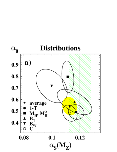
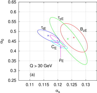
Figure 11: Left: $1$-$\sigma$ contours for simultaneous fits of $\alpha_{s}$ and $\alpha_{0}$ to $e^{+}e^{-}$ event-shape distributions. The error contours account for statistic, systematical and theoretical uncertainties. The shaded band indicates the result for $\alpha_{s}$ when using Monte Carlo hadronisation models. Figure taken from [184]. Right: $1$-$\sigma$ contours from fits to H1 DIS event shape distributions [115] with statistical and systematic errors added in quadrature. Figure taken from [33].

As was the case for mean values, a more systematic test involves carrying out a simultaneous fit of $\alpha_{s}$ and $\alpha_{0}$ for each observable and then checking for consistency between observables and with the corresponding results for mean values. Results from $e^{+}e^{-}$ and DIS are shown in figure 11, taken from [108, 184] and [33]. Other fits that have been carried out in recent years include [84, 89, 185].

Just as for the mean values, one notes that (with exception of $B_{W}$ and $M_{H}^{2}$ in $e^{+}e^{-}$, to be discussed shortly) there is good consistency between observables, both for $e^{+}e^{-}$ and DIS. This statement holds holds also for the EEC, fitted in [89], not shown in fig. 11. There is also good agreement with the results for the mean values, fig. 3, except marginally for DIS $\alpha_{s}$ results, which for distributions are in better accord with the world average.

The good agreement between distributions and mean values is important in the light of alternative approaches to fitting mean values, such as the RGI which, we recall, seems to suggest that the power correction for mean values can just as well be interpreted as higher order contributions. Were this really the case then one would expect to see no relation between $\alpha_{0}$ results for mean values and distributions.

Despite the generally good agreement, some problems do persist. Examining different groups’ results for the $\alpha_{s}$-$\alpha_{0}$ fits one finds that for some observables there is a large spread in the results. For example for the $e^{+}e^{-}$ $B_{T}$, ALEPH [84] find $\alpha_{s}=0.109\pm 0.007$ while the JADE result [184] shown in fig. 11 corresponds to $\alpha_{s}=0.116\pm 0.012$ (and this differs from a slightly earlier JADE result $\alpha_{s}=0.111\pm 0.006$ [108]). While the results all agree to within errors, those errors are largely theoretical and would be expected to be a common systematic on all results. In other words we would expect the results to be much closer together than $1$-$\sigma$. That this is not the case suggests that the fits might be unstable with respect to small changes in details of the fit, for example the fit range (as has been observed when including data in the range $20<Q<30$ in the fit corresponding to the right hand plot of figure 11 [33]). These differences can lead to contradictory conclusions regarding the success of the description of different observables and it would be of value for the different groups to work together to understand the origin of the differences, perhaps in a context such as the LEP QCD working group.

There do remain two cases however where there seems to be clear incompatibility between the data and theoretical prediction: the heavy-jet mass, $\rho_{H}$ (also referred to as $M_{H}^{2}$) and the wide-jet broadening, $B_{W}$. The heavy-jet mass is subject to $\Lambda/Q$ hadron mass effects, as discussed already in the context of mean values, however even after accounting for this by considering $p$ or $E$-scheme data, as has been done by DELPHI [89], the results appear to be rather inconsistent with other observables: $\alpha_{s}$ is too small and $\alpha_{0}$ too large, as for $B_{W}$, though less extreme. The common point between these two observables is that they both select the heavier/wider hemisphere and so are less inclusive than other observables. Studies with event generators [28] suggest that whereas for more inclusive observables the 2-jet limit of the shift works well even into the 3-jet region, for heavy-wide observables the 3-jet limit behaves very differently from the 2-jet limit and these differences becomes relevant even for relatively low values of the observable (some partially related discussion of the problem has been given also in [29]). We will come back to this and other potential explanations below when we discuss shape functions.

Beyond the ‘usual’ observables discussed above, there are some recent results also for the $C$-parameter shoulder at $C=3/4$, where [89] the shoulder position is seen to be consistent with a shift with the usual 2-jet coefficient $C_{C}=3\pi$ — this is in contradiction with the (smaller) result eq. (27) for the shift to the shoulder; however the analysis [89] doesn’t take into account resummation effects at the shoulder which may also contribute to an effective shift. A first analysis of corrections to the $y_{3}$ distribution has been given in [109] which shows evidence for $1/Q^{2}$ contributions in the $y_{3}$ distribution at the two lowest JADE centre of mass energies (14 and 22 GeV).

One last interesting point to discuss regarding the shift approximation for hadronisation is an application to the measurement of the QCD colour factors. The fact that the hadronisation is encoded via just a single parameter, with all the dependence on colour factors available explicitly for the perturbative and non-perturbative contributions, means that it is feasible to carry out a simultaneous fit not only for $\alpha_{s}$ and $\alpha_{0}$ but also for one or more of the QCD colour factors $C_{A}$, $C_{F}$ and $T_{R}$ [187]. This would have been much more difficult using Monte Carlo hadronisation because all the hadronisation parameters would have had to have been retuned for each change of the colour factors. The results for this fit are summarised and compared to other approaches in figure 12 [188], which shows $2$-$\sigma$ contours for $C_{F}$ and $C_{A}$. While other approaches constrain the ratio $C_{A}/C_{F}$, the event-shape approach gives by far the best independent measurement of $C_{A}$ and $C_{F}$. As a result the combination of the results gives rather tight limits on the colour factors, which are in good agreement with the QCD expectation.

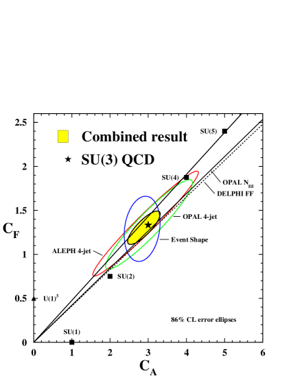
Figure 12: Determination of colour factors from resummed distributions with $1/Q$ (shift) power corrections and a variety of other methods. Figure taken from [188]. The ellipses show correlated measurements from studies of the angular distributions of 4-jet events [189, 190] and event shapes [187], while the lines are obtained from studies of the gluon fragmentation function [191] and from multiplicities in gluon jets [192].

5.2.2 Shape functions.

We have already mentioned that the approximation of a simple shift is valid only in the region $\Lambda/Q\ll v\ll 1$. To better understand the origin of the lower limit, let us expand eq. (32),

$$D_{\mathrm{NP},V}(v)=D_{\mathrm{PT},V}\left(v\right)+\sum_{n=1}^{\infty}(-1)^{n}\frac{(C_{V}{\cal P})^{n}}{n!}D_{\mathrm{PT},V}^{(n)}\left(v\right)$$ (34)

where $D_{\mathrm{PT},V}^{(n)}(v)$ is the $n^{\mathrm{th}}$ derivative of $D_{\mathrm{PT},V}(v)$ with respect to $v$. Since $D_{\mathrm{PT},V}^{(n)}(v)$ goes as $1/v^{n}$ one sees that when the shift $v\sim C_{V}{\cal P}$ all terms in the series are of the same order. While the $n=1$ term can be related to the power correction to the mean value of $V$, the shift merely provides an ansatz for the higher terms. The breakdown for small values of $vQ$ is clearly visible for the (DIS) thrust in fig. 10 (right).

A physically transparent way of dealing with the $n\geq 2$ terms has been developed by Korchemsky, Sterman and collaborators [121, 122, 193, 123, 124, 125]. One approximates $f_{V}(x,v,\alpha_{s},Q)$ in eq. (31) by a shape function [194] $\tilde{f}_{V}(x)$ (rather than the $\delta$-function which corresponds to a pure shift),

$$D_{\mathrm{NP},V}(v)=\int dx{\tilde{f}}_{V}(x)\,D_{\mathrm{PT},V}\left(v-\frac{x}{Q}\right).$$ (35)

In eq. (34), $(C_{V}P)^{n}$ is then replaced by ${\tilde{f}}_{n}/Q^{n}$ where ${\tilde{f}}_{n}$ is the $n^{\mathrm{th}}$ moment of ${\tilde{f}}_{V}(x)$.

There is considerable freedom in one’s choice of the form for the shape function. Accordingly, success in fitting a given event-shape distribution for any single value of $Q$ cannot, alone, be considered strong evidence in favour of the shape-function picture. The true test of the approach comes by determining the shape function at one value of $Q$ and then establishing whether it applies for all values of $Q$. This is illustrated for the $e^{+}e^{-}$ thrust in fig. 13 (left), where the following shape-function has been used [193, 123],

$$f(x)=\frac{2\left(x/\Lambda\right)^{a-1}}{\Lambda\Gamma\left(\frac{a}{2}\right)}\exp\left(-\frac{x^{2}}{\Lambda^{2}}\right)\,,$$ (36)

with two free parameters, $a$ and $\Lambda$ (it has been argued that the behaviour of this function for small $x$ and large $x$ is similar to that expected from a simple physical model for the dynamics at the origin of the shape function [125]). One notes the remarkable agreement, far into the two-jet region, for the whole range of $Q$ values.

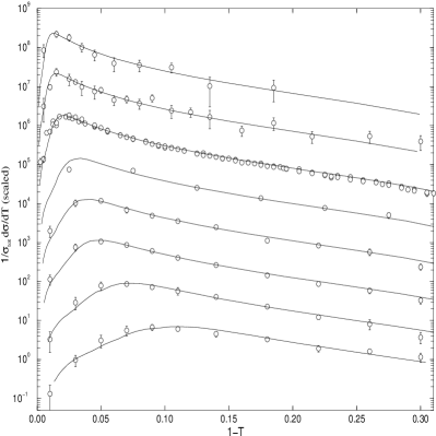
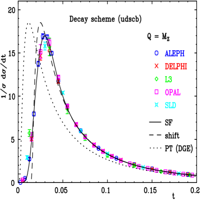
Figure 13: Left: the thrust distribution using the NLL+NLO perturbative distribution with the shape function eq. (36). Shown for $Q=14,22,35,44,55,91,133$ and $161$ GeV. Figure taken from [193]. Right: the thrust distribution at the perturbative (DGE) level, with a non-perturbative shift, and with a shape function. Figure taken from [29].

This is a clear success for the shape-function approach as compared to the simple shift discussed above. However the drawback of shape-functions is that a priori one loses all predictivity (save for the first moment) when going from one observable to another. This predictivity was one of the main strengths of the shift approach. Considerable work has therefore been devoted to understanding both the general properties of shape functions and the relations between shape functions of different observables.

One line of investigation has been to relate the shape functions for the thrust and heavy-jet mass ($\rho_{H}$) — this can be done with the help of the observation [56] that in the two-jet limit the thrust is just the sum of the light and heavy-jet (squared normalised) masses. In [124] Korchemsky and Tafat introduced a shape function ${\tilde{f}}(x_{1},x_{2})$ describing the distribution of non-perturbative radiation in each of the two hemispheres. The shape function for the thrust is then obtained by

$${\tilde{f}}_{T}(x)=\int dx_{1}dx_{2}\tilde{f}(x_{1},x_{2})\delta(x-x_{1}-x_{2}).$$ (37)

Instead for the heavy-jet mass one calculates the full (NP) double differential distribution for the two jet masses and from that derives the heavy-jet mass distribution (this is not quite equivalent to a simple shape-function for $\rho_{H}$). This approach gave a good fit to the thrust and heavy-jet mass data, on the condition that there was significant correlation between the non-perturbative contribution to the two hemispheres. It is difficult to interpret this result however, because as has already been mentioned, the default measurement scheme for the jet masses suffers from extra (universality-breaking) $\Lambda/Q$ corrections, and it is possible that in [124] these are being mimicked by inter-hemisphere correlations.

The thrust and heavy-jet mass have been investigated in great detail also by Gardi and Rathsman [70, 29]. In analogy with the approach for the mean thrust [138], they attempt not only to account for NLL+NLO and power correction contributions, but also for all (perturbative) enhanced effects associated with the running of the coupling, within a formalism that they refer to as Dressed Gluon Exponentiation (DGE). Among the interesting theoretical results (see also [139]) is that the renormalon analysis suggests that the second moment of the shape function should be precisely that expected from a pure shift (the same is true for the $C$-parameter [71]). This observation seems to be consistent with fits to the data, and would explain why the shift approximation works so well, at least for the relevant observables. The right-hand plot of fig. 13 shows the result of their analysis for the thrust, with both a shift and a shape-function. While the shape-function is clearly needed in the immediate vicinity of the peak and below, it is striking to see, above the peak, how well it is approximated by the shift.

One of the other interesting results in [29] relates to the analysis of the heavy-jet mass. In contrast to [124], a common hadron-mass scheme (decay-scheme) is used for the thrust and the heavy-jet mass, and there are no inter-hemisphere correlations in their shape function. Using the same parameters for the thrust and $\rho_{H}$ leads to reasonable fits, suggesting that the true inter-hemisphere correlations may actually be small. (A fit for $\rho_{H}$ alone does however prefer a lower value of $\alpha_{s}$ than for the thrust, as is seen also with the usual shifted NLL+NLO approach [89]).

A puzzle that emerges in the work of [70, 29] is that all the fits lead to quite small values of the coupling, $\alpha_{s}\simeq 0.109$ with a theoretical error of about $\pm 0.005$. A similarly low result was obtained in the analogous analysis of the mean thrust [138]. In contrast a study of $b$-fragmentation using dressed gluon exponentiation finds more standard values, $\alpha_{s}\simeq 0.118$ [195].

Let us close our discussion of shape functions with a recent result by Berger & Sterman [140]. Given that there are no simple relations between the shape functions for most common event shapes, they instead consider a new class of event shapes [65] whose definition involves a parameter $a$ which allows the nature of the event shape to be continuously varied from a broadening ($a=1$) to a thrust-type observable ($a=0$) and beyond. Their observation is that for all variants of the observable with $a<1$, the logarithm of any moment of the shape functions scales as $1/(1-a)$. In practice this scaling is found to hold in Monte Carlo studies of this class of observables — it would therefore be interesting to have data for these observables with which to make a comparison.

6 Outlook

Conceptually, event shapes are rather simple observables, yet they are sensitive to a range of characteristics of QCD radiation. This combination of theoretical simplicity and experimental sensitivity is perhaps one of the main reasons why event shapes have found so many applications. As we have seen, they provide vital inputs in studies of the ingredients of the QCD Lagrangian, such as the coupling and the colour factors; they play an important role in the tuning and testing of event generators; and they are at the heart of recent investigations into analytical approaches to understanding the dynamics of hadronisation.

There remain several directions in which progress may be expected (or at the very least hoped for) in coming years. All the experimental comparisons discussed here have been for event-shapes that vanish in the $2$-jet limit, yet there have been significant theoretical developments in recent years for observables that vanish also in the $3$-jet limit, examples being the $D$-parameter and thrust minor [18, 66, 32, 36, 34, 53, 45, 44, 46, 49]. Studies with jet rates [189] suggest that going to such ‘three-jet’ observables could reduce theoretical errors, though as discussed in [170] this needs to be investigated more systematically. Additionally three-jet observables will allow much more stringent tests of analytical hadronisation approaches since for the first time they introduce sensitivity to predictions about hadronisation from a gluon [18, 66], not just from a quark.

One of the frontiers of event shape studies is their extension to new processes. While $e^{+}e^{-}$ is the traditional domain for event-shape studies, we have seen that studies in DIS are in many respects competitive with $e^{+}e^{-}$ results. Additionally they provide important input on the question of universality of analytical hadronisation models, ruling out for example significant modifications of the hadronisation picture stemming from interactions with the proton remnant. Though so far the question has received only limited study, one interesting application of DIS studies would be in the use of event shapes for obtaining information on parton distribution functions, as suggested in [32].

Currently an option that is attracting growing experimental [37] and theoretical [36, 50, 38] interest is the development of event shapes in hadron-hadron collisions. Though much work remains to be done on this subject, it seems that the sensitivity to parton distributions will be somewhat stronger than in most DIS observables. Furthermore one expects a rich hadronisation structure associated both with the four-jet structure of hadronic dijet events and with the properties of the underlying event. It is to be hoped that the availability of automated resummation methods [38] will make the theoretical aspects of the study of new observables and processes more straightforward than has been the case in the past.

Another frontier on which progress is expected in near future is with respect to the accuracy of theoretical predictions. NNLO perturbative calculations are making rapid progress (for a recent review see [52]) with the main outstanding problem being that of a full subtraction procedure for combining zero, one and two-loop contributions and its implementation in a Monte Carlo integrator. Progress on NNLL resummations is also being made, albeit so far only in inclusive cases [196]. Though technically more involved, an extension to event shape resummations is certainly conceivable in the near future. Aside from the expected gains in accuracy that are the main motivation for these calculations, it will also be interesting to compare the exact higher-order calculations with predictions from approaches such as [70, 138, 161] which aim to identify the physically dominant higher-order contributions and in some cases [161, 89] claim to significantly reduce the theoretical uncertainties on $\alpha_{s}$.

Less predictable is what development can be expected on the subject of hadronisation corrections. As we have seen, much has been learnt from event-shape studies. Yet a variety of open questions remain. At a practical level it would for example be of interest to see an extension of the shape-function approach to a wider range of variables, including the quite subtle case of the broadenings and also to DIS event shapes. The wealth of DIS data at low $Q$, where shape functions are most important, makes the latter especially interesting.

There remain also important issues that are poorly understood even at the conceptual level. For example predictions are currently limited to the domain in which the event-shape is close to vanishing (e.g. $1-T$ in the $2$-jet limit). It is tempting to suggest that problems that persist for a couple of ‘recalcitrant’ observables (specifically, $\rho_{H}$, $B_{W}$) may actually be due to large differences between the power correction in the three-jet region (a significant part of the fit-range) and that in the well-understood two-jet limit (see e.g. fig. 3 of [109]). But techniques that would allow the calculation of the power correction to, say, the thrust or the broadening in the $3$-jet limit do not yet exist. Another (partially related) issue is that of anomalous dimensions — these have so far only been calculated for $\Lambda/Q$ effects that are associated with hadron masses [28]. Yet, as has been pointed out also in [197], they are bound to be present for all classes of power suppressed contributions. One clear physical origin for them is that soft-gluons (or hadrons) with transverse momenta of order $\Lambda$ are radiated not just from the $q\bar{q}$ system but also from all soft perturbative gluons with transverse momenta between $\Lambda$ and $Q$. Accounting for radiation from the latter will clearly lead to enhancements of power corrections by terms $(\alpha_{s}\ln Q/\Lambda)^{n}$. And a final point, not to be forgotten, is that most of the analytical hadronisation approaches are essentially perturbative methods ‘in disguise’. An understanding of how they really relate to hadronisation is very much lacking.

Let us close this review by remarking that one of the characteristics of event shape studies is that progress is made not merely through a better understanding of existing observables and data, but also through critical experimental studies of new observables with (supposedly!) better theoretical properties. The dialogue between experimenters and theorists is crucial in this respect. We look forward to its being as fruitful in coming years as it has been up to now.

References

References

- [1] J. R. Ellis, M. K. Gaillard and G. G. Ross, Nucl. Phys. B 111 (1976) 253 [Erratum-ibid. B 130 (1977) 516].
- [2] E. Farhi, Phys. Rev. Lett. 39 (1977) 1587.
- [3] H. Georgi and M. Machacek, Phys. Rev. Lett. 39 (1977) 1237.
- [4] G. C. Fox and S. Wolfram, Phys. Rev. Lett. 41 (1978) 1581; ibid., Nucl. Phys. B 149 (1979) 413 [Erratum-ibid. B 157 (1979) 543].
- [5] C. L. Basham, L. S. Brown, S. D. Ellis and S. T. Love, Phys. Rev. Lett. 41 (1978) 1585; C. L. Basham, L. S. Brown, S. D. Ellis and S. T. Love, Phys. Rev. D 19 (1979) 2018.
- [6] R. K. Ellis, W. J. Stirling and B. R. Webber, QCD and Collider Physics, Cambridge University Press, 1996.
- [7] D. J. Miller and M. H. Seymour, Phys. Lett. B 435 (1998) 199 [hep-ph/9805413].
- [8] D. J. Miller and M. H. Seymour, Phys. Lett. B 435 (1998) 213 [hep-ph/9805414]
- [9] B. R. Webber, in proceedings of the Summer School on Hadronic Aspects of Collider Physics, Zuoz, Switzerland, 1994, hep-ph/9411384.
- [10] G. Marchesini, B. R. Webber, G. Abbiendi, I. G. Knowles, M. H. Seymour and L. Stanco, Comput. Phys. Commun. 67 (1992) 465. G. Corcella et al., JHEP 0101 (2001) 010 [hep-ph/0011363].
- [11] T. Sjöstrand, Comput. Phys. Commun. 82 (1994) 74; T. Sjöstrand, P. Eden, C. Friberg, L. Lönnblad, G. Miu, S. Mrenna and E. Norrbin, hep-ph/0010017.
- [12] L. Lönnblad, Comput. Phys. Commun. 71 (1992) 15.
- [13] M. Beneke, Phys. Rept. 317 (1999) 1 [hep-ph/9807443].
- [14] S. Brandt, C. Peyrou, R. Sosnowski and A. Wroblewski, Phys. Lett. 12 (1964) 57.
- [15] L. Clavelli, Phys. Lett. B 85 (1979) 111; T. Chandramohan and L. Clavelli, Nucl. Phys. B 184 (1981) 365; L. Clavelli and D. Wyler, Phys. Lett. B 103 (1981) 383.
- [16] S. Catani, G. Turnock and B. R. Webber, Phys. Lett. B 295 (1992) 269.
- [17] D. P. Barber et al. [MARK-J COLLABORATION Collaboration], Phys. Rept. 63 (1980) 337.
- [18] A. Banfi, G. Marchesini, Y. L. Dokshitzer and G. Zanderighi, JHEP 0007 (2000) 002 [hep-ph/0004027]. A. Banfi, Y. L. Dokshitzer, G. Marchesini and G. Zanderighi, Phys. Lett. B 508 (2001) 269 [hep-ph/0010267].
- [19] A. De Rujula, J. R. Ellis, E. G. Floratos and M. K. Gaillard, Nucl. Phys. B 138 (1978) 387.
- [20] R. K. Ellis, D. A. Ross and A. E. Terrano, Nucl. Phys. B 178 (1981) 421.
- [21] G. Parisi, Phys. Lett. B 74 (1978) 65; J. F. Donoghue, F. E. Low and S. Y. Pi, Phys. Rev. D 20 (1979) 2759.
- [22] J. D. Bjorken and S. J. Brodsky, Phys. Rev. D 1 (1970) 1416; G. Hanson et al., Phys. Rev. Lett. 35 (1975) 1609.
- [23] C. Berger et al. [PLUTO Collaboration], Phys. Lett. B 82 (1979) 449.
- [24] W. Bartel et al. [JADE Collaboration], Z. Phys. C 33 (1986) 23.
- [25] S. Catani, Yu. L. Dokshitzer, M. Olsson, G. Turnock and B. R. Webber, Phys. Lett. B 269 (1991) 432.
- [26] S. Bethke, Z. Kunszt, D. E. Soper and W. J. Stirling, Nucl. Phys. B 370 (1992) 310 [Erratum-ibid. B 523 (1998) 681].
- [27] Y. L. Dokshitzer, G. D. Leder, S. Moretti and B. R. Webber, JHEP 9708 (1997) 001 [hep-ph/9707323].
- [28] G. P. Salam and D. Wicke, JHEP 0105 (2001) 061 [hep-ph/0102343].
- [29] E. Gardi and J. Rathsman, Nucl. Phys. B 638 (2002) 243 [hep-ph/0201019].
- [30] R. P. Feynman, Photon Hadron interactions, W. A. Benjamin, New York, 1972; R. D. Peccei and R. Ruckl, Nucl. Phys. B 162 (1980) 125; L. V. Gribov, Y. L. Dokshitzer, S. I. Troian and V. A. Khoze, Sov. Phys. JETP 67 (1988) 1303 [Zh. Eksp. Teor. Fiz. 94 (1988) 12].
- [31] K. H. Streng, T. F. Walsh and P. M. Zerwas, Z. Phys. C 2 (1979) 237.
- [32] A. Banfi, G. Marchesini, G. Smye and G. Zanderighi, JHEP 0111 (2001) 066 [hep-ph/0111157].
- [33] M. Dasgupta and G. P. Salam, JHEP 0208 (2002) 032 [hep-ph/0208073].
- [34] A. Banfi, G. Marchesini and G. Smye, JHEP 0204 (2002) 024 [hep-ph/0203150].
- [35] S. Catani, Y. L. Dokshitzer and B. R. Webber, Phys. Lett. B 285 (1992) 291.
- [36] A. Banfi, G. Marchesini, G. Smye and G. Zanderighi, JHEP 0108 (2001) 047 [hep-ph/0106278].
- [37] I. A. Bertram [D0 Collaboration], Acta Phys. Polon. B 33 (2002) 3141.
- [38] A. Banfi, G. P. Salam and G. Zanderighi, hep-ph/0304148; ibid. in preparation.
- [39] A. Banfi, hep-ph/0309161.
- [40] G. Sterman and S. Weinberg, Phys. Rev. Lett. 39 (1977) 1436.
- [41] P. Nason, unpublished, c. 1991.
- [42] W. T. Giele and E. W. Glover, Phys. Rev. D 46 (1992) 1980.
- [43] S. Catani and M. H. Seymour, Phys. Lett. B 378 (1996) 287 [hep-ph/9602277]; S. Catani and M. H. Seymour, Nucl. Phys. B 485 (1997) 291 [Erratum-imbid. B 510 (1997) 503] [hep-ph/9605323].
- [44] L. J. Dixon and A. Signer, Phys. Rev. D 56 (1997) 4031 [hep-ph/9706285]; A. Signer, Comput. Phys. Commun. 106 (1997) 125.
- [45] S. Weinzierl and D. A. Kosower, Phys. Rev. D 60 (1999) 054028 [hep-ph/9901277].
- [46] J. M. Campbell, M. A. Cullen and E. W. Glover, Eur. Phys. J. C 9 (1999) 245 [hep-ph/9809429].
- [47] E. Mirkes and D. Zeppenfeld, Phys. Lett. B 380 (1996) 205 [hep-ph/9511448].
- [48] D. Graudenz, hep-ph/9710244.
- [49] Z. Nagy and Z. Trocsanyi, Nucl. Phys. B 486 (1997) 189 [hep-ph/9610498]; Z. Nagy and Z. Trocsanyi, Phys. Rev. Lett. 79 (1997) 3604 [hep-ph/9707309]; Z. Nagy and Z. Trocsanyi, Phys. Rev. D 59 (1999) 014020 [Erratum-ibid. D 62 (2000) 099902] [hep-ph/9806317]; Z. Nagy and Z. Trocsanyi, Phys. Rev. Lett. 87 (2001) 082001 [hep-ph/0104315];
- [50] Z. Nagy, Phys. Rev. Lett. 88 (2002) 122003 [hep-ph/0110315]; Z. Nagy, hep-ph/0307268.
- [51] B. Potter, Comput. Phys. Commun. 133 (2000) 105 [hep-ph/9911221]; B. Potter, Comput. Phys. Commun. 119 (1999) 45 [hep-ph/9806437].
- [52] T. Gehrmann, hep-ph/0310178.
- [53] M. Dasgupta and G. P. Salam, Phys. Lett. B 512 (2001) 323 [hep-ph/0104277].
- [54] N. Brown and W. J. Stirling, Phys. Lett. B 252 (1990) 657. G. Leder, Nucl. Phys. B 497 (1997) 334 [hep-ph/9610552].
- [55] S. Catani, G. Turnock, B. R. Webber and L. Trentadue, Phys. Lett. B 263 (1991) 491.
- [56] S. Catani, L. Trentadue, G. Turnock and B. R. Webber, Nucl. Phys. B 407 (1993) 3.
- [57] S. Catani, G. Turnock and B. R. Webber, Phys. Lett. B 272 (1991) 368.
- [58] S. J. Burby and E. W. Glover, JHEP 0104 (2001) 029 [hep-ph/0101226].
- [59] Y. L. Dokshitzer, A. Lucenti, G. Marchesini and G. P. Salam, JHEP 9801 (1998) 011 [hep-ph/9801324].
- [60] S. Catani and B. R. Webber, Phys. Lett. B 427 (1998) 377 [hep-ph/9801350].
- [61] G. Dissertori and M. Schmelling, Phys. Lett. B 361 (1995) 167.
- [62] A. Banfi, G. P. Salam and G. Zanderighi, JHEP 0201 (2002) 018 [hep-ph/0112156].
- [63] Y. L. Dokshitzer and D. Diakonov, Phys. Lett. B 84 (1979) 234. G. Parisi and R. Petronzio, Nucl. Phys. B 154 (1979) 427. J. Kodaira and L. Trentadue, Phys. Lett. B 123 (1983) 335. J. C. Collins and D. E. Soper, Phys. Rev. Lett. 48 (1982) 655. P. E. Rakow and B. R. Webber, Nucl. Phys. B 187 (1981) 254.
- [64] Y. L. Dokshitzer, G. Marchesini and B. R. Webber, JHEP 9907 (1999) 012 [hep-ph/9905339].
- [65] C. F. Berger, T. Kucs and G. Sterman, Phys. Rev. D 68 (2003) 014012 [hep-ph/0303051].
- [66] A. Banfi, Y. L. Dokshitzer, G. Marchesini and G. Zanderighi, JHEP 0105 (2001) 040 [hep-ph/0104162].
- [67] V. Antonelli, M. Dasgupta and G. P. Salam, JHEP 0002 (2000) 001 [hep-ph/9912488].
- [68] M. Dasgupta and G. P. Salam, Eur. Phys. J. C 24 (2002) 213 [hep-ph/0110213].
- [69] R. Bonciani, S. Catani, M. L. Mangano and P. Nason, Phys. Lett. B 575 (2003) 268 [hep-ph/0307035].
- [70] E. Gardi and J. Rathsman, Nucl. Phys. B 609 (2001) 123 [hep-ph/0103217].
- [71] E. Gardi and L. Magnea, “The C parameter distribution in e+ e- annihilation,” JHEP 0308 (2003) 030 [hep-ph/0306094].
- [72] F. Krauss and G. Rodrigo, Phys. Lett. B 576 (2003) 135 [hep-ph/0303038].
- [73] S. Catani and B. R. Webber, JHEP 9710 (1997) 005 [hep-ph/9710333].
- [74] M. Dasgupta and G. P. Salam, JHEP 0203 (2002) 017 [hep-ph/0203009]; C. F. Berger, T. Kucs and G. Sterman, Phys. Rev. D 65 (2002) 094031 [hep-ph/0110004]; A. Banfi, G. Marchesini and G. Smye, JHEP 0208 (2002) 006 [hep-ph/0206076].
- [75] R. B. Appleby and M. H. Seymour, JHEP 0212 (2002) 063 [hep-ph/0211426]; R. B. Appleby and M. H. Seymour, JHEP 0309 (2003) 056 [hep-ph/0308086].
- [76] Y. L. Dokshitzer and G. Marchesini, JHEP 0303 (2003) 040 [hep-ph/0303101].
- [77] M. Dasgupta, hep-ph/0304086; R. B. Appleby and G. P. Salam, hep-ph/0305232.
- [78] H. Weigert, hep-ph/0312050.
-
[79]
I. H. Park et al. (AMY Collaboration),
Phys. Rev. Lett. 62 (1989) 1713;
Y. K. Li et al. (AMY Collaboration), Phys. Rev. D 41 (1990) 2675;
H. J. Behrend et al. (CELLO Collaboration), Z. Phys. C44 (1989) 63;
D. Bender et al. (HRS Collaboration), Phys. Rev. D 31 (1985) 1;
D. P. Barber et al. (Mark J Collaboration), Phys. Rev. Lett. 43 (1979) 830;
A. Petersen et al. (Mark II Collaboration), Phys. Rev. D 37 (1988) 1;
S. Bethke et al. (Mark II Collaboration), Z. Phys. C43 (1989) 325;
C. Berger et al. (PLUTO Collaboration), Z. Phys. C12 (1982) 297;
W. Braunschweig et al. (TASSO Collaboration), Phys. Lett. B214 (1988) 286;
W. Braunschweig et al. (TASSO Collaboration), Z. Phys. C45 (1989) 11;
W. Braunschweig et al. (TASSO Collaboration), Z. Phys. C47 (1990) 187;
I. Adachi et al. (TOPAZ Collaboration), Phys. Lett. B227 (1989) 495;
K. Nagai et al. (TOPAZ Collaboration), Phys. Lett. B278 (1992) 506;
Y. Ohnishi et al. (TOPAZ Collaboration), Phys. Lett. B313 (1993) 475. - [80] D. Decamp et al. [ALEPH Collaboration], Phys. Lett. B 255, 623 (1991).
- [81] D. Decamp et al. [ALEPH Collaboration], Phys. Lett. B 284, 163 (1992).
- [82] D. Buskulic et al. [ALEPH Collaboration], Z. Phys. C 73 (1997) 409.
- [83] R. Barate et al. [ALEPH Collaboration], Phys. Rept. 294 (1998) 1.
- [84] ALEPH Collaboration, “QCD Measurements in Annihilations at Centre-of-Mass Energies between 189 and 202 GeV”, ALEPH 2000-044 CONF 2000-027.
- [85] A. Heister et al. [ALEPH Collaboration], CERN-EP/2003-084; see also http://aleph.web.cern.ch/aleph/QCD/evsh.html.
- [86] P. Abreu et al. [DELPHI Collaboration], Z. Phys. C 73, 229 (1997).
- [87] P. Abreu et al. [DELPHI Collaboration], Phys. Lett. B 456, 322 (1999).
- [88] P. Abreu et al. [DELPHI Collaboration], Eur. Phys. J. C 14, 557 (2000) [hep-ex/0002026].
- [89] J. Abdallah et al. [DELPHI Collaboration], Eur. Phys. J. C 29 (2003) 285 [hep-ex/0307048].
- [90] O. Adriani et al. [L3 Collaboration], Phys. Lett. B 284, 471 (1992).
- [91] B. Adeva et al. [L3 Collaboration], Z. Phys. C 55 (1992) 39.
- [92] O. Adriani et al. [L3 Collaboration], Phys. Rept. 236, 1 (1993).
- [93] M. Acciarri et al. [L3 Collaboration], Phys. Lett. B 411, 339 (1997).
- [94] M. Acciarri et al. [L3 Collaboration], Phys. Lett. B 371, 137 (1996).
- [95] M. Acciarri et al. [L3 Collaboration], Phys. Lett. B 404, 390 (1997).
- [96] M. Acciarri et al. [L3 Collaboration], Phys. Lett. B 444, 569 (1998).
- [97] M. Acciarri et al. [L3 Collaboration], Phys. Lett. B 489, 65 (2000) [hep-ex/0005045].
- [98] P. Achard et al. [L3 Collaboration], Phys. Lett. B 536 (2002) 217 [hep-ex/0206052].
- [99] P. D. Acton et al. [OPAL Collaboration], Z. Phys. C 55 (1992) 1.
- [100] P. D. Acton et al. [OPAL Collaboration], Z. Phys. C 59, 1 (1993).
- [101] G. Alexander et al. [OPAL Collaboration], Z. Phys. C 72, 191 (1996).
- [102] K. Ackerstaff et al. [OPAL Collaboration], Z. Phys. C 75, 193 (1997).
- [103] G. Abbiendi et al. [OPAL Collaboration], Eur. Phys. J. C 16 (2000) 185 [hep-ex/0002012].
- [104] K. Abe et al. [SLD Collaboration], Phys. Rev. D 51 (1995) 962 [hep-ex/9501003].
- [105] P. A. Movilla Fernandez, O. Biebel, S. Bethke, S. Kluth and P. Pfeifenschneider [JADE Collaboration], Eur. Phys. J. C 1, 461 (1998) [hep-ex/9708034].
- [106] O. Biebel, P. A. Movilla Fernandez and S. Bethke [JADE Collaboration], Phys. Lett. B 459, 326 (1999) [hep-ex/9903009].
- [107] P. Pfeifenschneider et al. [JADE collaboration], Eur. Phys. J. C 17, 19 (2000) [hep-ex/0001055].
- [108] P. A. Movilla Fernandez, S. Bethke, O. Biebel and S. Kluth, Eur. Phys. J. C 22 (2001) 1 [hep-ex/0105059].
- [109] S. Kluth, M. Blumenstengel, P. A. Movilla Fernandez, S. Bethke, O. Biebel, C. Pahl and J. Schieck [JADE Collaboration], hep-ex/0305023.
- [110] J. Schieck [for the OPAL collaboration], hep-ex/0312036.
- [111] F. Yuasa et al., Prog. Theor. Phys. Suppl. 138 (2000) 18 [hep-ph/0007053].
- [112] A. Pukhov et al., hep-ph/9908288.
- [113] F. Krauss, R. Kuhn and G. Soff, JHEP 0202 (2002) 044 [hep-ph/0109036].
- [114] C. Adloff et al. [H1 Collaboration], Phys. Lett. B 406 (1997) 256 [hep-ex/9706002].
- [115] C. Adloff et al. [H1 Collaboration], Eur. Phys. J. C 14 (2000) 255 [Addendum-ibid. C 18 (2000) 417] [hep-ex/9912052].
- [116] H. U. Martyn [H1 Collaboration], hep-ex/0010046.
- [117] S. Chekanov et al. [ZEUS Collaboration], Eur. Phys. J. C 27 (2003) 531 [hep-ex/0211040].
- [118] J. Breitweg et al. [ZEUS Collaboration], Phys. Lett. B 421 (1998) 368 [hep-ex/9710027].
- [119] B. R. Webber, Nucl. Phys. Proc. Suppl. 71 (1999) 66 [hep-ph/9712236].
- [120] A. V. Manohar and M. B. Wise, Phys. Lett. B 344 (1995) 407 [hep-ph/9406392].
- [121] G. P. Korchemsky and G. Sterman, Nucl. Phys. B 437 (1995) 415 [hep-ph/9411211].
- [122] G. P. Korchemsky and G. Sterman, hep-ph/9505391.
- [123] G. P. Korchemsky and G. Sterman, Nucl. Phys. B 555 (1999) 335 [hep-ph/9902341].
- [124] G. P. Korchemsky and S. Tafat, JHEP 0010 (2000) 010 [hep-ph/0007005].
- [125] A. V. Belitsky, G. P. Korchemsky and G. Sterman, Phys. Lett. B 515 (2001) 297 [hep-ph/0106308].
- [126] M. Beneke and V. M. Braun, Nucl. Phys. B 454 (1995) 253 [hep-ph/9506452].
- [127] B. R. Webber, Phys. Lett. B 339 (1994) 148 [hep-ph/9408222].
- [128] Y. L. Dokshitzer and B. R. Webber, Phys. Lett. B 352 (1995) 451 [hep-ph/9504219].
- [129] Y. L. Dokshitzer, G. Marchesini and B. R. Webber, Nucl. Phys. B 469 (1996) 93 [hep-ph/9512336].
- [130] Y. L. Dokshitzer and B. R. Webber, Phys. Lett. B 404 (1997) 321 [hep-ph/9704298].
- [131] R. Akhoury and V. I. Zakharov, Nucl. Phys. B 465 (1996) 295 [hep-ph/9507253].
- [132] R. Akhoury and V. I. Zakharov, Phys. Lett. B 357 (1995) 646 [hep-ph/9504248].
- [133] Y. L. Dokshitzer, A. Lucenti, G. Marchesini and G. P. Salam, Nucl. Phys. B 511 (1998) 396 [Erratum-ibid. B 593 (2001) 729] [hep-ph/9707532].
- [134] Y. L. Dokshitzer, A. Lucenti, G. Marchesini and G. P. Salam, JHEP 9805 (1998) 003 [hep-ph/9802381].
- [135] Y. L. Dokshitzer, G. Marchesini and G. P. Salam, Eur. Phys. J. directC 1 (1999) 3 [hep-ph/9812487].
- [136] M. Dasgupta, L. Magnea and G. Smye, JHEP 9911 (1999) 025 [hep-ph/9911316].
- [137] G. E. Smye, JHEP 0105 (2001) 005 [hep-ph/0101323].
- [138] E. Gardi and G. Grunberg, JHEP 9911 (1999) 016 [hep-ph/9908458].
- [139] E. Gardi, JHEP 0004 (2000) 030 [hep-ph/0003179].
- [140] C. F. Berger and G. Sterman, JHEP 0309 (2003) 058 [hep-ph/0307394].
- [141] C. W. Bauer, C. Lee, A. V. Manohar and M. B. Wise, hep-ph/0309278.
- [142] C. W. Bauer, A. V. Manohar and M. B. Wise, Phys. Rev. Lett. 91 (2003) 122001 [hep-ph/0212255].
- [143] Z. Trocsanyi, JHEP 0001 (2000) 014 [hep-ph/9911353].
- [144] M. Dasgupta and B. R. Webber, Eur. Phys. J. C 1 (1998) 539 [hep-ph/9704297].
- [145] M. Dasgupta and B. R. Webber, JHEP 9810 (1998) 001 [hep-ph/9809247].
- [146] G. P. Salam and Z. Trócsányi, Limited Automated Predictor of Power Suppressed Effects (LAPPSE), unpublished work.
- [147] B. R. Webber, hep-ph/9510283.
- [148] Y. L. Dokshitzer, “Why It Seems Too Early To Report On Status Of QCD,” Given at International School of Subnuclear Physics: 31th Course: From Supersymmetry to the Origin of Space-Time, Erice, Italy, 4-12 Jul 1993
- [149] P. Boucaud, J. P. Leroy, J. Micheli, H. Moutarde, O. Pene, J. Rodriguez-Quintero and C. Roiesnel, Nucl. Phys. Proc. Suppl. 106 (2002) 266 [hep-ph/0110171].
- [150] P. Nason and M. H. Seymour, Nucl. Phys. B 454 (1995) 291 [hep-ph/9506317].
- [151] R.P. Feynman, ‘Photon Hadron Interactions’, W.A. Benjamin, New York (1972).
- [152] P. A. Movilla Fernandez, Nucl. Phys. Proc. Suppl. 74 (1999) 384 [hep-ex/9808005].
- [153] B. R. Webber, Nucl. Phys. Proc. Suppl. 71 (1999) 66 [hep-ph/9712236].
- [154] G. Zanderighi, private communication.
- [155] G. J. McCance, hep-ph/9912481.
- [156] P. Nason and B. R. Webber, Phys. Lett. B 395 (1997) 355 [arXiv:hep-ph/9612353].
- [157] S. Banerjee (L3), private communication.
- [158] A. Dhar and V. Gupta, Phys. Rev. D 29 (1984) 2822.
- [159] B. R. Webber, JHEP 9810 (1998) 012 [hep-ph/9805484].
- [160] E. Gardi and G. Grunberg, Nucl. Phys. Proc. Suppl. 86 (2000) 426 [hep-ph/9909226].
- [161] J. M. Campbell, E. W. N. Glover and C. J. Maxwell, Phys. Rev. Lett. 81 (1998) 1568 [hep-ph/9803254]. D. T. Barclay, C. J. Maxwell and M. T. Reader, Phys. Rev. D 49 (1994) 3480.
- [162] M. Beneke, Phys. Lett. B 307 (1993) 154.
- [163] P. Abreu et al. (DELPHI Collaboration), Z. Phys. C73 (1996) 11.
- [164] D. Buskulic et al. (ALEPH Collaboration), Z. Phys. C55 (1992) 209.
- [165] I. G. Knowles et al., “QCD Event Generators,” hep-ph/9601212.
- [166] S. Frixione and B. R. Webber, JHEP 0206 (2002) 029 [hep-ph/0204244]. S. Frixione, P. Nason and B. R. Webber, JHEP 0308 (2003) 007 [hep-ph/0305252].
- [167] S. Gieseke, A. Ribon, M. H. Seymour, P. Stephens and B. Webber, hep-ph/0311208.
- [168] LEP QCD working group, work in progress.
- [169] H. Stenzel, hep-ex/0309061.
- [170] S. Bethke, Nucl. Phys. Proc. Suppl. 121 (2003) 74 [hep-ex/0211012].
- [171] K. Hagiwara et al. [Particle Data Group Collaboration], Phys. Rev. D 66 (2002) 010001.
- [172] R. W. L. Jones, M. Ford, G. P. Salam, H. Stenzel and D. Wicke, JHEP 0312 (2003) 007 [hep-ph/0312016].
- [173] P. M. Stevenson, Phys. Rev. D 23 (1981) 2916.
- [174] G. Grunberg, Phys. Rev. D 29 (1984) 2315.
- [175] S. J. Brodsky, G. P. Lepage and P. B. Mackenzie, Phys. Rev. D 28 (1983) 228.
- [176] P. Abreu et al. [DELPHI Collaboration], Phys. Lett. B 418 (1998) 430.
- [177] G. Abbiendi et al. [OPAL Collaboration], Eur. Phys. J. C 21 (2001) 411 [hep-ex/0105046].
- [178] A. Brandenburg, P. N. Burrows, D. Muller, N. Oishi and P. Uwer, Phys. Lett. B 468 (1999) 168 [hep-ph/9905495].
- [179] R. Barate et al. [ALEPH Collaboration], Eur. Phys. J. C 18 (2000) 1 [hep-ex/0008013].
- [180] P. Bambade, M. J. Coster, J. Fuster and P. Tortosa, Delphi conference note 2003-022-CONF-642 (unpublished).
- [181] W. Bernreuther, A. Brandenburg and P. Uwer, Phys. Rev. Lett. 79 (1997) 189 [hep-ph/9703305].
- [182] G. Rodrigo, A. Santamaria and M. S. Bilenky, Phys. Rev. Lett. 79 (1997) 193 [hep-ph/9703358].
- [183] P. Nason and C. Oleari, Nucl. Phys. B 521 (1998) 237 [hep-ph/9709360].
- [184] P. A. Movilla Fernandez, hep-ex/0209022.
- [185] T. Kluge, hep-ex/0310063.
- [186] G. P. Salam and G. Zanderighi, Nucl. Phys. Proc. Suppl. 86 (2000) 430 [hep-ph/9909324].
- [187] S. Kluth, P. A. Movilla Fernandez, S. Bethke, C. Pahl and P. Pfeifenschneider, Eur. Phys. J. C 21 (2001) 199 [hep-ex/0012044].
- [188] S. Kluth, hep-ex/0309070.
- [189] A. Heister et al. [ALEPH Collaboration], Eur. Phys. J. C 27 (2003) 1.
- [190] G. Abbiendi et al. [OPAL Collaboration], Eur. Phys. J. C 20 (2001) 601 [hep-ex/0101044].
- [191] P. Abreu et al. [DELPHI Collaboration], Eur. Phys. J. C 13 (2000) 573.
- [192] G. Abbiendi et al. [OPAL Collaboration], Eur. Phys. J. C 23 (2002) 597 [hep-ex/0111013].
- [193] G. P. Korchemsky, hep-ph/9806537.
-
[194]
G. Sterman,
Nucl. Phys. B 281 (1987) 310;
S. Catani and L. Trentadue, Nucl. Phys. B 327 (1989) 323;
S. Catani and L. Trentadue, Nucl. Phys. B 353 (1991) 183;
G. P. Korchemsky, Mod. Phys. Lett. A 4 (1989) 1257;
G. P. Korchemsky and G. Marchesini, Phys. Lett. B 313 (1993) 433;
I. I. Y. Bigi, M. A. Shifman, N. G. Uraltsev and A. I. Vainshtein, Int. J. Mod. Phys. A 9 (1994) 2467 [hep-ph/9312359];
R. D. Dikeman, M. A. Shifman and N. G. Uraltsev, Int. J. Mod. Phys. A 11 (1996) 571 [hep-ph/9505397];
M. Neubert, Phys. Rev. D 49 (1994) 3392 [hep-ph/9311325];
M. Neubert, Phys. Rev. D 49 (1994) 4623 [hep-ph/9312311];
G. P. Korchemsky and G. Sterman, Phys. Lett. B 340 (1994) 96 [hep-ph/9407344];
A. G. Grozin and G. P. Korchemsky, Phys. Rev. D 53 (1996) 1378 [hep-ph/9411323]. - [195] M. Cacciari and E. Gardi, Nucl. Phys. B 664 (2003) 299 [hep-ph/0301047].
- [196] G. Bozzi, S. Catani, D. de Florian and M. Grazzini, Phys. Lett. B 564 (2003) 65 [hep-ph/0302104].
- [197] L. Magnea, hep-ph/0211013.