Magnetic Moments of Baryons with a Single Heavy Quark

Abstract

We calculate the magnetic moments of heavy baryons with a single heavy quark in the bound-state approach. In this approach the heavy baryons is considered as a heavy meson bound in the field of a light baryon. The light baryon field is represented as a soliton excitation of the light pseudoscalar and vector meson fields. For these calculations we adopt a model that is both chirally invariant and consistent with the heavy quark spin symmetry. We gauge the model action with respect to photon field in order to extract the electromagnetic current operator and obtain the magnetic moments by computing pertinent matrix elements of this operator between the bound state wavefunctions. We compare our predictions for the magnetic moments with results of alternative approaches for the description of heavy baryon properties.

1 Introduction

There has been recent interest to study properties of baryons that contain heavy quarks. In particular the development of the heavy quark or Isgur-Wise symmetry [1] has generated many studies [2]–[7] on the spectrum of baryons with a single heavy quark in the so–called bound state approach. To set the notation for what we consider a baryon with a single heavy quark we denote heavy quarks (charm or bottom) by “$Q$” and light quarks (up or down) by “$q$”. In the quark language a baryon whose properties we wish to explore has the structure $qqQ$. This defines the quantum numbers of the considered baryon. In general, of course, the structure of such a baryon may be more complicated because additional quark–antiquark–pairs may be excited. In the above mentioned bound state approach the heavy baryon is considered as a heavy spin multiplet of mesons (with structure $Q\bar{q}$) bound in the field of the nucleon, or more generally a light baryon of $qqq$–structure. As suggested by the $1/N_{\rm C}$ expansion [8, 9] of QCD the field of the nucleon emerges as a soliton configuration of light meson fields of $q\bar{q}$ structure. Reviews of the soliton approach to the light baryons are given in refs. [10]–[14] while the bound state approach for the “light” hyperons is discussed in refs. [15]–[18].

The basic idea is to consider an effective meson model that includes both, light degrees of freedom and mesons that contain a heavy quark. In such a model the light components of the heavy meson fields couple the light meson fields according to the rules of chiral symmetry. Thus this it permits not only an expansion of heavy baryon properties in powers of $1/M$, $1/N_{\rm C}$ [19] but also in the number of derivatives acting on the light components of the heavy system. However, this introduces a large number of unknown parameters in the model Lagrangian. We therefore find it more compelling to employ a model with light vector mesons ($\rho$ and $\omega$) to construct the soliton rather than a model with many derivatives of the light pseudoscalar fields. Actually the need for light vector mesons is not surprising since, in the soliton approach, they are necessary to explain, for example, the neutron–proton mass difference [20], the nucleon axial singlet matrix element [21] and the “high–energy” behavior of phase shifts in meson–baryon scattering [12]. Furthermore heavy quark components of the heavy meson field are required to exhibit the heavy quark symmetry as the masses tend to infinity, i.e. spin and flavor independent interactions. Therefore the model also requires both heavy pseudoscalar and heavy vector meson fields. Based on a model [22] that reflects all those features, the heavy baryon mass splittings have been discussed [23], obtaining satisfactory agreement with experiment. Also pentaquarks of structure $qqq{\bar{Q}}q$ have been considered in this model as antimesons (${\bar{Q}}q$) bound in the field of the soliton.

Here we will go one step further and study magnetic moments of baryons with a single heavy quark in the model suggested in ref. [22] as an example for computing static properties. This not only requires to construct the soliton of the light meson fields, to compute the heavy meson bound state wavefunction, and to quantize the the combined system to generate states to be identified as heavy baryons but in addition also to derive of the electromagnetic current 19.12. operator in the model and to subsequently evaluate matrix elements thereof between heavy baryon states. It is important to note that both the light and the heavy sector of the model will contribute to that current and hence to the magnetic moments of heavy baryons. Stated otherwise, these magnetic moments directly vary with the parameters of the light sector and not only indirectly via the soliton profiles as e.g. the spectrum of the heavy baryons does.

This paper is organized as follows. In section 2 we will review the model Lagrangian for both the light and heavy flavor sectors of the model. This will also provide the opportunity to derive covariant expressions for the electromagnetic current. Section 2 also contains a brief discussion the soliton profiles that emerge in the light flavor sector as well the heavy meson bound state profiles. In section 3 we will generate states with good baryon quantum numbers by canonically quantizing collective coordinates that parameterize the (zero–mode) rotations of the combined soliton – heavy meson system. This makes mandatory the discussion of field components that are absent classically but get induced by the collective rotation. Section 4 represents the major progress for the studies of heavy baryons as a heavy meson bound to a soliton as we construct the magnetic moment operator in this model and compute the corresponding matrix elements numerically. Concluding remarks are to be found in section 5. Also we complete the paper by including an appendix that summarizes functionals of the meson profiles that emerge along the computation.

Some preliminary results of this study have already been presented in a conference contribution [24].

2 The model Lagrangian

The model Lagrangian can be divided in two distinct parts. The first part, ${\cal L}_{\rm light}$ describes the interaction of the mesons that are built out of the light quarks up and down. Our model not only contains the pseudoscalar pion fields but also the vector mesons $\omega$ and $\rho$. The interactions among these light mesons is dictated by chiral symmetry. The second part, ${\cal L}_{\rm heavy}$ in addition contains fields that correspond to mesons that are built out of a single heavy quark (charm or bottom) and light quarks. This part of the Lagrangian is consistent with the heavy quark spin flavor symmetry and therefore contains both pseudoscalar and vector degrees of freedom. In the charm quark sector these are $D(1865)$ and $D^{\ast}(2007)$ while $B(5279)$ and $B^{\ast}(5325)$ contain a bottom quark.

The Lagrangian ${\cal L}_{\rm light}$ contains (topological) soliton solutions that are identified with baryons according to the Skyrme–model picture. Substituting this soliton configuration for the light meson fields in ${\cal L}_{\rm heavy}$ generates a potential for the heavy meson fields. The Klein–Gordon equation associated with this potential has solutions with energy less than the rest mass of the considered heavy mesons, i.e. a bound heavy meson. We combine bound heavy mesons with the soliton of the light mesons (i.e. the soliton represents a baryon of light quarks) to obtain representatives for baryons with a single heavy quark. In the soliton description this model for the heavy baryon is that of a heavy meson bound to a light baryon. In this section we will review how this picture emerges and also discuss the basics for computing the magnetic moments of such heavy baryons.

2.1 The light meson Lagrangian

The light sector of the model is given by the chirally invariant Lagrangian discussed in refs. [25, 28]. In addition to the standard Skyrme model, which considers pseudoscalar pion fields only, this Lagrangian also contains vector meson degrees of freedom. In order to efficiently incorporate chiral symmetry it is most useful to employ the non–linear representation of the isovector pion fields ($\vec{\pi}$) via the chiral field $U={\rm exp}\left(i\vec{\pi}\cdot\vec{\tau}/f_{\pi}\right)$ where $f_{\pi}=93{\rm MeV}$ and $\vec{\tau}$ are the pion decay constant and the Pauli matrices, respectively. To begin with, a chirally invariant Lagrangian for vector mesons should contain both, vector and axialvector fields. The chirally covariant elimination of the axialvector introduces the root, $\xi$ of the chiral field, i.e. $\xi^{2}=U$ [28] as well as vector and axialvector currents of the pion fields:

$$v_{\mu}=\frac{i}{2}\left(\xi{\partial_{\mu}}{\xi^{\dagger}}+{\xi^{\dagger}}{\partial_{\mu}}{\xi}\right),\qquad p_{\mu}=\frac{i}{2}\left(\xi{\partial_{\mu}}{\xi^{\dagger}}-{\xi^{\dagger}}{\partial_{\mu}}{\xi}\right)\,.$$ (1)

We comprise the isoscalar $\omega$ and the isovector $\vec{\rho}$ within a single matrix field $\rho_{\mu}=(\vec{\rho\,}_{\mu}\cdot\vec{\tau}+\omega_{\mu}{\mbox{{\sf 1}\rule{0.39993pt}{6.58746pt}}})/2$ and further define

$$F_{\mu\nu}(\rho)=\partial_{\mu}\rho_{\nu}-\partial_{\nu}\rho_{\mu}+ig[\rho_{\mu},\rho_{\nu}]\qquad{\rm and}\qquad R_{\mu}=\rho_{\mu}-\frac{1}{g}v_{\mu}$$ (2)

to compactly write the normal parity part of the Lagrangian for the light mesons

$${\cal L}_{S}=f_{\pi}^{2}{\rm tr}\left[p_{\mu}p^{\mu}\right]+\frac{1}{4}m_{\pi}^{2}f_{\pi}^{2}{\rm tr}\left[U+U^{\dagger}-2\right]-\frac{1}{2}{\rm tr}\left[F_{\mu\nu}(\rho)F^{\mu\nu}(\rho)\right]+m_{\rm V}^{2}{\rm tr}\left[R_{\mu}R^{\mu}\right]\,.$$ (3)

Here $m_{\pi}=138{\rm MeV}$ and $m_{\rm V}=770{\rm MeV}$ are pion and vector meson masses, respectively. The last term in eq. (3) contains the tri–linear vertex $\vec{\rho}_{\mu}\cdot\left(\vec{\pi}\times\partial^{\mu}\vec{\pi}\right)$ and allows to determine the coupling constant $g\approx 5.6$ from the decay $\rho\to\pi\pi$. In addition the light meson Lagrangian contains a part that involves the Levi-Cevita tenor $\epsilon_{\mu\nu\alpha\beta}$. Since this part includes the nonlocal Wess–Zumino–Witten term it is most convenient to write it in action form using differential forms like $p=p_{\mu}dx^{\mu}$

$$\Gamma_{an}(p,R,F) = \frac{2N_{C}}{15\pi^{2}}\int{\rm tr}[p^{5}]$$

$$+\int{\rm tr}\left[\frac{4i}{3}\left(\gamma_{1}+\frac{3}{2}\gamma_{2}\right)Rp^{3}-\frac{g}{2}\gamma_{2}F(\rho)(pR-Rp)-2ig^{2}(\gamma_{2}+2\gamma_{3})R^{3}p\right].$$

Note that we will only consider the physical case of $N_{C}=3$ color degrees of freedom.

In ref. [25] two of the three unknown constants $\gamma_{1,2,3}$ were determined from purely strong interaction processes. Defining $\tilde{h}=-\frac{2\sqrt{2}}{3}\gamma_{1}$, $\tilde{g}_{VV\phi}=g\gamma_{2}$ and $\kappa=\frac{\gamma_{3}}{\gamma_{2}}$ the central values $\tilde{h}=0.4$ and $\tilde{g}_{VV\phi}=1.9$ were found. Within experimental uncertainties (stemming from the uncertainty in the $\omega-\phi$ mixing angle) these may vary in the range $\tilde{h}=-0.15,..,0.7$ and $\tilde{g}_{VV\phi}=1.3,..,2.2$ subject to the constraint $|\tilde{g}_{VV\phi}-\tilde{h}|\approx 1.5$. The third parameter, $\kappa$ could not be fixed in the meson sector, however, from the study [25] of nucleon properties in the $U(2)$ reduction of the model it was argued that $\kappa\approx 1$. To be specific, we will always employ the parameters:

$$g=5.6\,,\quad\tilde{h}=0.3\,,\quad\tilde{g}_{{\rm VV}\phi}=1.8\,,\quad\kappa=1.2\,.$$ (4)

that have been found suitable for describing the low–lying baryons for three light flavors [30].

The total action for the light mesons is the sum

$$\Gamma_{\rm light}[\xi,\rho]=\int d^{4}x{\cal L}_{S}+\Gamma_{\rm an}\,.$$ (5)

The electromagnetic current associated with $\Gamma_{\rm light}$ is most easily obtained by gauging it with the photon field ${\cal A}_{\mu}\,{\cal Q}$ where ${\cal Q}={\rm diag}(2/3,-1/3)$ is the quark charge matrix and extracting the linear term:

$${\cal J}_{\mu}^{\rm light}=\frac{\delta\Gamma[\xi,\rho,{\cal A}]}{\delta{\cal A}^{\mu}}\Big{|}_{{\cal A}=0}\,.$$ (6)

This yields

$${\cal J}_{\mu}^{\rm light} = f_{\pi}^{2}{\rm tr}\left\{{\cal Q}\left[\xi^{\dagger}p_{\mu}\xi-\xi p_{\mu}\xi^{\dagger}\right]\right\}-\frac{m_{V}^{2}}{g}{\rm tr}\left\{{\cal Q}\left[\xi R_{\mu}\xi^{\dagger}+\xi^{\dagger}R_{\mu}\xi\right]\right\}$$ (14)

$$-\frac{2i}{3}\left[\frac{N_{c}}{4\pi^{2}}-\frac{1}{g}\left(\gamma_{1}+\frac{3}{2}\gamma_{2}\right)\right]\epsilon_{\mu\nu\rho\sigma}{\rm tr}\left\{\left[\xi^{\dagger}{\cal Q}\xi+\xi{\cal Q}\xi^{\dagger}\right]p^{\nu}p^{\rho}p^{\sigma}\right\}$$

$$-\frac{2i}{3}\left(\gamma_{1}+\frac{3}{2}\gamma_{2}\right)\epsilon_{\mu\nu\rho\sigma}{\rm tr}\left\{\left[\xi^{\dagger}{\cal Q}\xi-\xi{\cal Q}\xi^{\dagger}\right]\left[R^{\nu}p^{\rho}p^{\sigma}+p^{\nu}p^{\rho}R^{\sigma}-p^{\nu}R^{\rho}p^{\sigma}\right]\right\}$$

$$-\frac{g}{4}\gamma_{2}\epsilon_{\mu\nu\rho\sigma}{\rm tr}\left\{{\cal Q}\left(\xi\left[F^{\nu\rho}R^{\sigma}+R^{\nu}F^{\rho\sigma}-\frac{1}{g}\left(F^{\nu\rho}p^{\sigma}+p^{\nu}F^{\rho\sigma}\right)\right]\xi^{\dagger}\right.\right.$$

$$\left.\left.\qquad\qquad\mp\xi^{\dagger}\left[F^{\nu\rho}R^{\sigma}+R^{\nu}F^{\rho\sigma}+\frac{1}{g}\left(F^{\nu\sigma}p^{\rho}+p^{\nu}F^{\rho\sigma}\right)\right]\xi\right)\right\}$$

$$-ig^{2}\left(\gamma_{2}+2\gamma_{3}\right)\epsilon_{\mu\nu\rho\sigma}{\rm tr}\left\{{\cal Q}\left(\xi\left[R^{\nu}R^{\rho}R^{\sigma}-\frac{1}{g}\left(R^{\nu}R^{\rho}p^{\sigma}+p^{\nu}R^{\rho}R^{\sigma}-R^{\nu}p^{\rho}R^{\sigma}\right)\right]\xi^{\dagger}\right.\right.$$

$$\left.\left.\qquad\qquad-\xi^{\dagger}\left[R^{\nu}R^{\rho}R^{\sigma}+\frac{1}{g}(R^{\nu}R^{\rho}p^{\sigma}+p^{\nu}R^{\rho}R^{\sigma}-R^{\nu}p^{\rho}R^{\sigma})\right]\xi\right)\right\}$$

$$+2d_{1}\epsilon_{\mu\nu\rho\sigma}\partial^{\nu}\{{\rm tr}\left\{{\cal Q}\left[\xi\left(R^{\rho}p^{\sigma}-p^{\rho}R^{\sigma}\right)\xi^{\dagger}+\xi^{\dagger}\left(R^{\rho}p^{\sigma}-p^{\rho}R^{\sigma}\right)\xi\right]\right\}\,.$$

The last term, proportional to $d_{1}$ has no analogue in the pure hadronic part of the action (2.1). This term is of electromagnetic nature and the coupling constant can be related to the light vector meson decay $\omega\rightarrow\pi^{0}\gamma$: $|2d_{1}-\frac{\gamma_{2}}{2}|=0.038\pm 0.002$ [26].

2.2 Solitons

The action for the light degrees of freedom contains static solition solutions. The hedgehog type configuration reads [25]:

$$U(\vec{r\,}) = \exp\left(i\vec{r}\cdot\vec{\tau\,}F(r)\right)\,\quad,{\it i.e.}\quad\xi(\vec{r\,})=\exp\left(i\vec{r}\cdot\vec{\tau\,}\frac{F(r)}{2}\right)\,$$ (15)

$$\rho^{a}_{i}(\vec{r\,}) = \frac{G(r)}{gr}\epsilon_{ija}\hat{r}_{j}\tau_{a}\,,\quad{\rm and}\quad\omega(\vec{r\,})=\frac{\omega(r)}{g}\,,$$ (16)

while all other field components vanish classically. These configurations are invariant under combined spatial and flavor rotations generated by the vector sum $\vec{L}+\vec{S}+\vec{I}$, the so–called grand spin. Assuming the boundary conditions (a prime indicates the derivative with respect to $r$)

$$F(0)=\pi\,,\quad G(0)=-2\,,\quad\omega^{\prime}(0)=0\,,\quad F(\infty)=G(\infty)=\omega(\infty)=0$$ (17)

yields baryon number one solitons by substituting the ansätze (16) into the action (5) and extremizing the resulting functional of the classical mass, $M_{\rm cl}[F,G,\omega]$. For completeness we list the explicit form of that functional in the appendix. Note, that this soliton does not yet describe baryon states with good spin and flavor quantum numbers. Before describing the cranking procedure that generates such states, we will focus on that part of the model Lagrangian that contains the heavy meson fields.

2.3 The relativistic Lagrangian for the heavy mesons

The relativistic Lagrangian ${\cal L}_{\rm heavy}$ which describes the coupling between light and heavy mesons is given by [22]:

$${\cal L}_{\rm heavy} = D_{\mu}P(D^{\mu}P)^{\dagger}-\frac{1}{2}Q_{\mu\nu}(Q^{\mu\nu})^{\dagger}-M^{2}PP^{\dagger}+M^{\ast 2}Q_{\mu}Q^{\mu\dagger}$$ (18)

$$+ 2iMd\left(Pp_{\mu}Q^{\mu\dagger}-Q_{\mu}p^{\mu}P^{\dagger}\right)-\frac{d}{2}\epsilon^{\alpha\beta\mu\nu}\left[Q_{\nu\alpha}p_{\mu}Q_{\beta}^{\dagger}+Q_{\beta}p_{\mu}(Q_{\nu\alpha})^{\dagger}\right]$$ (19)

$$- \frac{2\sqrt{2}icM}{m_{V}}\left\{2Q_{\mu}F^{\mu\nu}(\rho)Q_{\nu}^{\dagger}-\frac{i}{M}\epsilon^{\alpha\beta\mu\nu}\left[D_{\beta}PF_{\mu\nu}(\rho)Q_{\alpha}^{\dagger}+Q_{\alpha}F_{\mu\nu}(\rho)(D_{\beta}P)^{\dagger}\right]\right\}\,.$$ (20)

Here the mass $M$ of the heavy pseudoscalar Meson $P$ differs from the mass $M^{\ast}$ of the heavy vector meson $Q_{\mu}$. We take

$$M = 1865\>MeV\,{\rm(D-meson)}\,,\quad 5279\>MeV\,{\rm(B-meson)},$$ (21)

$$M^{\ast} = 2007\>MeV\,{\rm(D-meson)}\,,\quad 5325\>MeV\,{\rm(B-meson)}\,.$$ (22)

It should be noticed that the heavy meson fields are conventionally defined as row vectors in isospin space. The chirally covariant derivatives of the heavy fields $P$ and $Q$ and the field-strength tensor $Q_{\mu\nu}$ are defined as:

$$D_{\mu}P^{\dagger} = \left[\partial_{\mu}-i\alpha g\rho_{\mu}-i\left(1-\alpha\right)v_{\mu}\right]P^{\dagger}=\left[\partial_{\mu}-iv_{\mu}-ig\alpha R_{\mu}\right]P^{\dagger}\,,$$ (23)

$$D_{\mu}Q_{\nu}^{\dagger} = \left[\partial_{\mu}-iv_{\mu}-ig\alpha R_{\mu}\right]Q_{\nu}^{\dagger}\,,\quad(Q_{\mu\nu})^{\dagger}=D_{\mu}Q_{\nu}^{\dagger}-D_{\nu}Q_{\mu}^{\dagger}.$$ (25)

In eq. (20) we have two sets of two terms each that involve the identical coupling constants $d$ and $c$. Each of these terms is chirally invariant and could thus in principle carry independent coupling constants. However, the condition that the Lagrangian ${\cal L}_{\rm heavy}$ obeys the heavy quark spin symmetry in the limit $M,M^{\ast}\to\infty$ requires the combination of these terms as given in eq. (20) [22]. Note however, that we do not assume infinitely large masses for the heavy meson. The coupling constants $d$, $c$ and $\alpha$ are still not precisely determined. While $d$ and $c$ can be determined from the decay widths of the heavy mesons [29]

$$d=0.53\,,\qquad c=1.60\,,$$ (26)

there is no direct experimental information for the value of $\alpha$. The value of $\alpha$ would be unity if a possible definition of light vector meson dominance for the electromagnetic form factors of the heavy meson was adopted [29].

Due to the electromagnetic gauging of the Lagrangian extra terms appear in the light vector fields $\rho_{\mu}$, $v_{\mu}$ and $p_{\mu}$. The respective electromagnetic and chirally invariant forms read (we choose the electric charge to be unity):

$$\tilde{\rho}_{\mu}=\rho_{\mu}-\frac{1}{g}{\cal Q}{\cal A}_{\mu}\,,\quad\tilde{v}_{\mu}=v_{\mu}+\frac{1}{2}{\cal A}_{\mu}\left(\xi{\cal Q}\xi^{\dagger}+\xi^{\dagger}{\cal Q}\xi-2{\cal Q}\right)\quad{\rm and}\quad\tilde{p}_{\mu}=p_{\mu}-\frac{1}{2}{\cal A}_{\mu}\left(\xi{\cal Q}\xi^{\dagger}-\xi^{\dagger}{\cal Q}\xi\right)\,.$$ (27)

Considering these extra terms, the electromagnetic and chiral covariant derivative of the heavy meson fields has to be modified:

$$D_{\mu}P^{\dagger} = \left(\partial_{\mu}-i\alpha g\tilde{\rho}_{\mu}-i\left(1-\alpha\right)\tilde{v}_{\mu}-i\left({\cal Q}-{\cal C}\right){\cal A}_{\mu}\right)P^{\dagger}$$ (28)

$$= \left(\partial_{\mu}-i\alpha g\rho_{\mu}-i\left(1-\alpha\right)v_{\mu}+ie{\cal A}_{\mu}\left[{\cal C}-\frac{1}{2}\left(1-\alpha\right)\left(\xi{\cal Q}\xi^{\dagger}+\xi^{\dagger}{\cal Q}\xi\right)\right]\right)P^{\dagger}\,,$$ (29)

which makes plausible the above assertion that $\alpha=1$ corresponds to vector meson dominance because for that value there is only the direct coupling to the heavy mesons. The charge of the heavy quark in question is denoted by $\cal C$, i.e. ${\cal C}=\frac{2}{3}$ for the charm sector and ${\cal C}=-\frac{1}{3}$ for the bottom sector. Finally we substitute eq. (29), for $D_{\mu}P^{\dagger}$, its analogue for $(D_{\mu}Q_{\mu})^{\dagger}$ as well as $\tilde{\rho}$, etc. from eq. (27) for $\rho$ into the Lagrangian (20) to obtain the electromagnetic current of the heavy mesons

$${\cal J}_{\mu}^{\rm heavy}=\left.\frac{\delta{\cal L}_{\rm heavy}}{\delta{\cal A}^{\mu}}\right|_{{\cal A}_{\mu}=0} = i\left(P\tilde{C}\left(D_{\mu}P\right)^{\dagger}-D_{\mu}P\tilde{C}P^{\dagger}\right)+i\left(Q^{\nu}\tilde{C}Q_{\mu\nu}^{\dagger}-Q_{\mu\nu}\tilde{C}Q^{\nu\dagger}\right)$$ (34)

$$-ieMd\left(P\left(\xi{\cal Q}\xi^{\dagger}-\xi^{\dagger}{\cal Q}\xi\right)Q_{\mu}^{\dagger}-Q_{\mu}\left(\xi{\cal Q}\xi^{\dagger}-\xi^{\dagger}{\cal Q}\xi\right)P\right)$$

$$-id\epsilon_{\alpha\beta\mu\nu}\left(Q^{\alpha}\tilde{C}p^{\nu}Q^{\beta\dagger}-Q^{\beta}p^{\nu}\tilde{C}Q^{\alpha\dagger}\right.$$

$$\quad\left.+\frac{i}{4}\left[Q^{\nu\alpha}\left(\xi{\cal Q}\xi^{\dagger}-\xi^{\dagger}{\cal Q}\xi\right)Q^{\beta\dagger}+Q^{\beta}\left(\xi{\cal Q}\xi^{\dagger}-\xi^{\dagger}{\cal Q}\xi\right)Q^{\nu\alpha\dagger}\right]\right)$$

$$+i\frac{2\sqrt{2}c}{m_{V}}\epsilon_{\alpha\beta\mu\nu}\left(P\tilde{C}F^{\beta\nu}(\rho)Q^{\alpha\dagger}-Q^{\alpha}F^{\beta\nu}(\rho)\tilde{C}P^{\dagger}\right)\,.$$

Here the abbreviation $\tilde{C}={\cal C}-\frac{1-\alpha}{2}\left(\xi{\cal Q}\xi^{\dagger}+\xi^{\dagger}{\cal Q}\xi\right)$ has been employed. A similar electromagnetic current was also derived in ref. [29] to discuss radiative decays of heavy vector mesons. However, the $d$–type term in eq. (34) was omitted as it does not contribute to such processes.

2.4 Bound states

Substituting the soliton configuration (16) for the light meson fields in ${\cal L}_{\rm heavy}$ generates a potential for the heavy meson fields. The existence of heavy meson bound states in this potential has been established some time ago [23]. Such bound states emerge for both, positive and negative frequency modes. The former correspond to mesons bound to the light quark soliton and thus carry quantum numbers of ordinary three–quark baryons. The latter, however, have antimesons bound to the soliton and their quantum numbers cannot be constructed in a three–quark picture. Rather additional quark–antiquark excitations are required and the resulting heavy baryons possess pentaquark structures.

In the current study we want to compute the magnetic moments of ground state baryons with a single heavy quark, i.e. $\Lambda_{c},\Sigma_{c}$ when the heavy meson is a D–meson and $\Lambda_{b},\Sigma_{b}$ in the case of the B–meson. The ground states, of course, correspond to the most tightly bound state. Due to the hedgehog structure of the background soliton, which has nonzero orbital angular momentum, these bound states emerge in the $P$–wave channels, rather than in the $S$–wave as naïvly assumed. For that reason we will only consider the $P$–wave channel and refer to ref. [23] for details on $S$–wave channel bound states. The appropriate ansatz for the heavy meson multiplet in the P-wave channel reads:

$$P^{\dagger}(\vec{r\,},t) = \frac{1}{\sqrt{4\pi}}\Phi(r)\hat{r}\cdot\vec{\tau}\,\rho(\epsilon)\,{\rm e}^{i\epsilon t}\,,\quad Q_{0}^{\dagger}(\vec{r\,},t)=\frac{1}{\sqrt{4\pi}}\Psi_{0}(r)\,\rho(\epsilon)\,{\rm e}^{i\epsilon t}\,,$$ (35)

$$Q_{i}^{\dagger}(\vec{r\,},t) = \frac{1}{\sqrt{4\pi}}\left[i\Psi_{1}(r)\hat{r}_{i}+\frac{1}{2}\Psi_{2}(r)\epsilon_{ijk}\hat{r}_{j}\tau_{k}\right]\,\rho(\epsilon)\,{\rm e}^{i\epsilon t}\,.$$ (36)

Here $\rho(\epsilon)=\begin{pmatrix}\rho_{1}(\epsilon)\cr\rho_{2}(\epsilon)\end{pmatrix}$ refers to a properly normalized isospinor describing the isospin of the the heavy meson multiplet. Upon canonical quantization the Fourier amplitudes $\rho(\epsilon)$ and $\rho^{\dagger}(\epsilon)$ are elevated to annihilation and creation operators for a heavy meson quantum with the energy eigenvalue $\epsilon$ (see below). We substitute the field configurations (16) and (36) into the Lagrangian given by eqs. (5) and (20) and integrate over coordinates to obtain the Lagrange function of the form

$$L=-M_{cl}[F,G,\omega]+I_{\epsilon}[F,G,\omega;\Phi,\Psi_{0},\Psi_{1},\Psi_{2}]\rho^{\dagger}(\epsilon)\rho(\epsilon)\,.$$ (37)

Here $M_{cl}$ denotes the classical solition mass. Its variation yields the profile functions $F$, $G$ and $\omega$. The heavy meson fields are contained in the functional $I_{\epsilon}$ where the subscript indicates the parameterical dependence on the frequency of the fluctuation heavy meson fields. The explicit expressions for the functionals $M_{cl}$ and $I_{\epsilon}$ are given in the appendix. We vary $I_{\epsilon}$ with respect to $\Phi,\Psi_{0},\Psi_{1}$ and $\Psi_{2}$ to get the equations of motions for the heavy meson fields. These constitute Klein–Gordon type equations with potentials generated by the profile functions $F$, $G$ and $\omega$. We then tune the frequency $\epsilon$ such that these equations yield a normalizable solution with $|\epsilon|<M$. The solution with the smallest such $|\epsilon|$ is the bound state we are looking for. The equations of motions for the heavy meson fields are homogeneous linear differential equations. Hence they provide a solution only up to an overall prefactor. Nonetheless, the equations of motion for the heavy meson fields allow us to extract a metric for a scalar product between different bound states. In particular its diagonal elements can be used to properly normalize the bound state wave functions. The physical interpretation of the normalization condition is that each occupation of the bound state should add the amount $|\epsilon|$ to the total energy and that such a bound states carries unit heavy flavor. Thus we obtain the normalization condition

$$\left|\frac{\partial}{\partial{\epsilon}}I_{\epsilon}[\Phi,\Psi_{0},\Psi_{1},\Psi_{2}]\right|=1$$ (38)

in addition to the canonical commutation relation $[\rho_{i}(\epsilon),\rho_{j}^{\dagger}(\epsilon^{\prime})]=\delta_{ij}\delta_{\epsilon,\epsilon^{\prime}}$ for the Fourier amplitude of the bound state. For further details we again refer to ref. [23].

3 States with Spin and Flavor Quantum Numbers

It is easy to verify that the field configurations for both the light mesons and the heavy mesons are neither eigenfunctions of the spin nor the isospin generators. It is the aim of this section to construct such eigenstates for the bound state system.

3.1 Collective coordinates

We employ the cranking procedure in order to generate states that correspond to physical baryons. In a first step we introduce collective coordinates that parameterize the (iso-) spin orientation of the meson configuration,

$$\xi(\vec{r\,},t)=A(t)\xi_{H}(\vec{r\,})A^{\dagger}(t),\qquad\rho_{i}(\vec{r\,},t)=A(t)\rho_{i\>H}(\vec{r\,})A^{\dagger}(t).$$ (39)

The time dependence of the collective rotations is measured by the angular velocities $\vec{\Omega\,}$:

$$A^{\dagger}(t)\frac{d}{dt}A(t)=\frac{i}{2}\vec{\tau}\cdot\vec{\Omega}\,.$$ (40)

In addition to the collective rotation of the soliton configuration, classically vanishing field components are induced. In the case of the light vector mesons these are given by [26]:

$$\omega_{i}=\frac{1}{g}\varphi(r)\epsilon_{ijk}\Omega_{j}\hat{r}_{k}\,,\quad\rho_{0}^{k}=\frac{1}{g}\left[\xi_{1}(r)\Omega_{k}+\xi_{2}(r)\hat{r}\cdot\vec{\Omega}\hat{r}_{k}\right]\,\,.$$ (41)

After introducing these additional fields the Lagrangian for the light mesons now contains a term which is quadratic in the angular velocities. The constant of proportionality defines the moment of inertia $\alpha^{2}[F,G,\omega;\xi_{1},\xi_{2},\varphi]$. Varying this moment of inertia with respect to the radial functions $\xi_{1}(r)$, $\xi_{2}(r)$ and $\varphi(r)$ yields their equations of motion that are linear, inhomogeneous second order differential equations with the inhomogeneity defined by the classical profile functions $F,G$ and $\omega$. We solve these differential equations subject to boundary conditions that avoid singularities in both the respective equations of motion and the moment of inertia [26]. The moment of inertia as evaluated for this solution is a pure number. For the parameters listed above eq (4) we find $\alpha^{2}=5.01\,{\rm GeV^{-1}}$.

The heavy meson fields also need to be rotated in isospin space, this is done analogously to eq.(39):

$$P^{\dagger}\rightarrow A(t)P^{\dagger},\qquad Q_{\mu}^{\dagger}\rightarrow A(t)Q_{\mu}^{\dagger}\,.$$ (42)

We have now summarized all the collectively rotating fields and are in the position to give the Lagrange function for the collective coordinates Lagrangian ${\cal L}_{\rm light}+{\cal L}_{\rm heavy}$,

$$L_{\rm coll}=-M_{cl}+I_{\epsilon}\rho^{\dagger}\rho+\frac{\alpha^{2}}{2}\vec{\Omega\,}^{2}+\frac{\chi}{2}\rho^{\dagger}\vec{\Omega}\cdot\vec{\tau\,}\rho$$ (43)

that is obtained by integrating ${\cal L}_{\rm light}+{\cal L}_{\rm heavy}$ with the above ansätze substituted. The new quantity is $\chi$ which describes the coupling between the collective rotations and the bound state wave functions. For reasons that will become obvious below, we will refer to $\chi$ as the hyperfine parameter. It is a functional of all radial functions, i.e. it contains both light and heavy meson fields and can straightforwardly be computed once a value for $\alpha$ is chosen, cf. table 1.

The quantization of the Lagrangian (43) proceeds along the bound state approach to the Skyrmion [15]–[18]: Noether charges for spin and flavor have to be constructed. Considering the variation of the fields under infinitesimal symmetry transformations, we find for the isospin transformation transformation:

$$\left[\Phi,i\frac{\tau_{i}}{2}\right]=-D_{ij}(A)\frac{\partial\dot{\Phi}}{\partial\Omega_{j}}+...\,.$$ (44)

Here $\Phi$ refers to any of the given iso-rotating meson fields and the ellipses represent subleading terms in $1/N_{C}$, e.g. time derivatives of the angular velocities which might arise from eq. (41). Furthermore $D_{ij}(A)={1/2}\;tr[\tau_{i}A\tau_{j}A^{\dagger}]$ denotes the adjoint representation of the collective rotations $A$. It is straightforward to conclude from eq. (44) that the total isospin is related to the derivative of the Lagrange function with respect to the angular velocities:

$$I_{i}=-D_{ij}(A)\frac{\partial L}{\partial\Omega_{j}}\,.$$ (45)

The total spin operator $\vec{J}$ contains the grand spin operator $\vec{G}$,

$$G_{i}=J_{i}+D_{ij}^{-1}(A)I_{j}=J_{i}-J_{i}^{sol}\,,$$ (46)

with $\vec{J}^{sol}=\partial L/\partial\vec{\Omega}$. As a consequence of eq. (45) we obtain the relation:

$$(\vec{J}^{sol})^{\>2}=\vec{I}^{\,\,2}=I(I+1).$$ (47)

By construction the light meson fields do not contribute to the grand spin $\vec{G}$. Also those parts of the heavy meson wave functions (42) that are placed between the collective coordinates $A$ and the spinor $\rho$ carry zero grand spin. With the normalization condition (38) one therefore finds for the grandspin operator:

$$\vec{G}=-\rho^{\dagger}\frac{\vec{\tau}}{2}\rho.$$ (48)

This relation connects the operator multiplying the hyperfine parameter in the collective Lagrangian in eq. (43) to the spin and isospin operators. The collective coordinate piece of the Hamiltonian is then obtained from the Legendre transformation:

$$H_{\rm coll}=\vec{\Omega}\cdot\vec{J}^{sol}-L_{\rm coll}=\frac{1}{2\alpha^{2}}\left(\vec{J}^{sol}+\chi\vec{G}\right)^{2}\,.$$ (49)

Since the moment of inertia, $\alpha^{2}$ is of order $N_{C}$, this operator is of order $1/N_{C}$. Finally the mass formula for baryon $B$ with a single heavy quark reads:

$$M_{B}=M_{cl}+|\epsilon|+\frac{1}{2{\alpha^{2}}}\left[\chi J(J+1)+(1-\chi)I(I+1)\right].$$ (50)

Contributions of $O(\chi^{2})$ have been omitted for consistency since these terms are quartic in the heavy meson wavefunctions and have been excluded form the model form the very beginning. Obviously the parameter $\chi$ characterizes the hyperfine splitting. In ref. [23] it has been verified that it vanishes in heavy quark limit $M$, $M^{\ast}\rightarrow\infty$ . This is a consequence of heavy quark spin symmetry that predicts hadrons to be degenerate that only differ by their spin quantum number.

To constrain the unknown parameter $\alpha$ we compute the mass differences of the bound P—wave heavy baryons $\Sigma_{C}$ and $\Sigma_{C}^{\ast}$ to $\Lambda_{C}$. In addition, we calculate the mass differences of $\Lambda_{C}$ to the nucleon and $\Lambda_{B}$. A more detailed comparison containing also S–Wave bound states and radially excited states can be found in ref. [23]. For quite a range of $\alpha$ fair agreement with the empirical data is obtained. The $\Sigma_{C}-\Lambda_{C}$ mass differences suggest a negative value of $\alpha$ while the experimental mass difference between the nucleon and the $\Lambda_{C}$ is reproduced for $\alpha\approx 0.4$. The $\Lambda_{B}-\Lambda_{C}$ mass difference is off by only about 5%.

Table 1: Quantities that enter the mass formula (50) as functions of the unknown parameter $\alpha$. The other model parameters are as in eqs. (4, 22) and (26). The binding energy is defined as $\omega=M-|\epsilon|$, $M$ being the mass of the heavy pseudoscalar meson. We also compare the resulting mass differences to experimental data in cases the latter are available [31]. The superscripts denote the heavy quark flavor under consideration. Energies are measured in MeV and masses are displayed relative to $\Lambda_{C}$.

$\alpha$	-0.3	0.0	0.1	0.2	0.3	0.4	0.5	0.6	0.7	0.8	exp.
$\omega^{C}$	615	548	526	504	483	461	439	418	397	376
$\omega^{B}$	872	797	773	748	724	699	675	651	626	602
$\chi^{C}$	0.165	0.140	0.132	0.123	0.114	0.105	0.096	0.087	0.078	0.069
$\chi^{B}$	0.060	0.053	0.050	0.046	0.045	0.042	0.039	0.037	0.034	0.031
$\Delta M_{\Sigma_{C}}$	167	171	173	175	177	178	180	182	184	186	168
$\Delta M_{\Sigma_{C}}^{\ast}$	216	214	213	212	211	210	209	208	207	207	235
$\Delta M_{N}$	-1187	-1252	-1274	-1295	-1316	-1337	-1358	-1379	-1399	-1419	-1344
$\Delta M_{\Lambda_{B}}$	3164	3172	3173	3176	3178	3181	3182	3185	3188	3191	3339$\pm$9

In the framework of collective coordinate quantization baryon wavefunctions emerge as Wigner–$D$ functions of the collective coordinates. These wavefunctions enter the computation of the magnetic moments to be discussed in the next section. For baryons without heavy flavor components these wavefunctions read

$${\bf\Psi}_{N}(I=J,I_{3},J,J_{3})={\cal N}D_{I_{3},-J_{3}}^{(I=J)}(A)\,,$$ (51)

while for the baryons with a single heavy quark component we need to couple a diquark state ($J^{sol}$ is integer) of collective coordinates with unit occupation of the bound state that carries half–integer spin ($\vec{J}-\vec{J}^{sol}=\vec{G}$)

$${\bf\Psi}_{B}(I,I_{3},J,J_{3})={\cal N}^{\prime}\sum_{J_{3}^{sol},G_{e}}C^{J\>J_{3}}_{I\>J_{3}^{sol},\>\frac{1}{2}\>G_{3}}D_{I_{3},-J_{3}^{sol}}^{I=J^{sol}}(A)|\frac{1}{2},G_{3}\rangle$$ (52)

to total spin according to eq. (46). In the above equations, $C$ is a Clebsch–Gordan coefficient while ${\cal N}$ and ${\cal N}^{\prime}$ are suitable normalization constants.

4 Electromagnetic current and results for magnetic moments

In this section we compute the magnetic moments from matrix elements of the electromagnetic current operator given in eqs. (14) and (34). The defining equation for the magnetic moment operator reads

$$\hat{\mu}=\frac{1}{2}\epsilon_{3ij}\int d^{3}r\,x_{i}\left({\cal J}^{\rm light}_{j}+{\cal J}^{\rm heavy}_{j}\right)\,.$$ (53)

We now substitute the field configurations (16), (36), (41) and (42) into eqs. (14) and (34). We then obtain the operator as sum of terms that are products of integrals over the profile functions and operators that act in the space of the collective coordinates ($A$) and/or as creation and annihilation operators ($\rho$) for the heavy meson bound state,

$$\hat{\mu}=\mu_{S,0}\alpha^{2}\Omega_{3}-\mu_{V,0}D_{33}(A)+\mu_{S,1}\rho^{\dagger}\frac{\tau_{3}}{2}\rho-\mu_{V,1}D_{33}(A)\rho^{\dagger}\rho\,.$$ (54)

We omit the energy argument of the spinor $\rho$, it is understood to be the bound state energy $\epsilon$ The first two terms in eq. (54) do not contain the bound state wavefunction and are those already considered for the two flavor version of the model in ref. [26]. Note that for convenience we factorized the moment of inertia, $\alpha^{2}$ for the isoscalar piece to make contact with the notation in refs. [16, 17]. From eq. (14) we find for this isoscalar piece,

$$\mu_{S,0} = -\frac{8\pi M_{\rm N}}{9\alpha^{2}}\int{drr^{2}}\Bigg{\{}\frac{2m_{V}^{2}}{g^{2}}\phi+\left[\frac{N_{C}}{4\pi^{2}}-\frac{1}{g}(\gamma_{1}+\frac{3}{2}\gamma_{2})\right]F^{\prime}\sin^{2}{F}$$ (58)

$$\hskip 56.9055pt+\frac{1}{2g}\gamma_{2}\left(\sin{F}(G^{\prime}-\xi^{\prime}_{1})+F^{\prime}[G(1-\xi_{1})+\xi_{2}]\right)$$

$$\hskip 56.9055pt+\frac{1}{2g}(\gamma_{2}+2\gamma_{3})F^{\prime}(\xi_{1}-1+\cos{F})(1+G-\cos{F})$$

$$\hskip 56.9055pt+2d_{1}\left[F^{\prime}(\xi_{1}+\xi_{2})-\frac{2}{r}\sin{F}(2+G-\xi_{1}-2\cos{F})\right]\Bigg{\}}\,,$$

while the explicit form of the isovector piece reads

$$\mu_{V,0} = \frac{8\pi M_{\rm N}}{3}\int{drr^{2}}\Bigg{\{}f_{\pi}^{2}\sin^{2}{F}-\frac{m_{V}^{2}}{g^{2}}\cos{F}(1+G-\cos{F})$$ (62)

$$\hskip 56.9055pt+\frac{1}{g}(\gamma_{1}+\frac{3}{2}\gamma_{2})\omega F^{\prime}\sin^{2}{F}-\frac{1}{2g}(\gamma_{2}+2\gamma_{3})F^{\prime}\omega\cos{F}(1+G-\cos{F})$$

$$\hskip 56.9055pt+\frac{1}{2g}\gamma_{2}\sin{F}[\omega^{\prime}(1+G-2\cos{F})-G^{\prime}\omega]$$

$$\hskip 56.9055pt+2d_{1}\left[F^{\prime}\omega+\frac{2}{r}\omega\sin{F}\cos{F}\right]\Bigg{\}}\,.$$

For the parameter set (4) we find numerically $\mu_{S,0}=0.43\,{\rm n.m}$ and $\mu_{V,0}=6.70\,{\rm n.m.}$. On the other hand $\mu_{S,1}$ and $\mu_{V,1}$ are bilinear in the heavy meson bound state wavefunctions. Again, there are isoscalar

$$\mu_{S,1} = -\frac{8M_{N}}{3}\left({\cal C}-\frac{1}{6}\left(1-\alpha\right)\right)\int{drr^{2}}\Bigg{\{}\Phi^{2}\left(1+\frac{R_{\alpha}}{2}\right)$$ (65)

$$+\frac{1}{2}\left[\Psi_{0}\left(R_{\alpha}\Psi_{0}+\left(\epsilon-\frac{\alpha\omega}{2}\right)r\Psi_{2}\right)+\Psi_{2}^{2}\left(1+\frac{R_{\alpha}}{2}\right)-\Psi_{1}\left(\Psi_{2}^{\prime}r+\Psi_{2}+R_{\alpha}\Psi_{1}\right)\right]$$

$$-\frac{d}{2}\Psi_{0}\left(\Psi_{1}\sin{F}-\Psi_{2}\frac{F^{\prime}r}{2}\right)-\frac{\sqrt{2}c}{m_{V}g}\Phi\left(\Psi_{2}\omega^{\prime}r-2\Psi_{0}G^{\prime}\right)\Bigg{\}}\,,$$

and isovector contributions

$$\mu_{V,1} = \frac{2M_{N}}{3}\left(1-\alpha\right)\int{drr^{2}}\cos{F}\Bigg{\{}\Phi_{2}^{2}\left(1+\frac{R_{\alpha}}{2}\right)$$ (70)

$$+\frac{1}{2}\left[-\Psi_{0}\left(R_{\alpha}\Psi_{0}+\left(\epsilon-\frac{\alpha\omega}{2}\right)r\Psi_{2}\right)+\Psi_{2}^{2}\left(1+\frac{R_{\alpha}}{2}\right)+\Psi_{1}\left(\Psi_{2}^{\prime}r+\Psi_{2}+R_{\alpha}\Psi_{1}\right)\right]$$

$$+d\,\Psi_{0}\Psi_{1}\sin{F}-\frac{\sqrt{2}c}{m_{V}g}\Phi\left(\Psi_{2}\omega^{\prime}r-2\Psi_{0}G^{\prime}\right)\Bigg{\}}$$

$$+\frac{dM_{N}}{3}\int{drr^{2}}\Big{\{}r\left(\Psi_{0}\Psi_{2}^{\prime}-\Psi_{0}^{\prime}\Psi_{2}\right)+\Psi_{0}\Psi_{2}+2R_{\alpha}\Psi_{0}\Psi_{1}$$

$$\hskip 85.35826pt+2r\left(\epsilon-\frac{\alpha\omega}{2}\right)\Psi_{1}\Psi_{2}-2Mr\sin{F}\Psi_{2}\Phi\Big{\}}\,,$$

with $R_{\alpha}=$ $\cos{F}-1+\alpha\left(1+G-\cos{F}\right)$. The factor $M_{N}=940{\rm MeV}$ enters because we measure the magnetic moments in nucleon magnetons [n.m.]. Numerical results for both the charm and the bottom sectors are displayed in table 2.

Table 2: Numerical results for the coefficients in the magnetic moment operator (54) that contain the bound state wavefunctions. Data are given units of nucleon magnetons (n.m.). See also table 1.

$\alpha$	-0.3	0.0	0.1	0.2	0.3	0.4	0.5	0.6	0.7	0.8
	Charm Sector
$\mu_{S,1}$	-0.168	-0.186	-0.191	-0.197	-0.203	-0.208	-0.214	-0.219	-0.225	-0.230
$\mu_{V,1}$	-0.037	-0.037	-0.038	-0.038	-0.038	-0.039	-0.039	-0.040	-0.040	-0.041
	Bottom Sector
$\mu_{S,1}$	0.070	0.063	0.061	0.059	0.057	0.054	0.052	0.050	0.048	0.046
$\mu_{V,1}$	-0.006	-0.006	-0.005	-0.004	-0.003	-0.003	-0.002	-0.002	-0.001	-0.001

We now sandwich the operator (54) between the states listed in eqs. (51) and (52) to obtain the magnetic moment of a given baryon as linear combinations of the functionals $\mu_{S,0}$, …,$\mu_{V,1}$. This yields [16, 17]:

$$\mu(p) = \frac{1}{2}\mu_{S,0}+\frac{1}{3}\mu_{V,0}$$

$$\mu(n) = \frac{1}{2}\mu_{S,0}-\frac{1}{3}\mu_{V,0}$$

$$\mu(\Lambda_{Q}) = \frac{1}{2}\tilde{\mu}_{S,1}$$

$$\mu(\Sigma_{Q}^{I_{3}=+1}) = \frac{2}{3}\mu_{S,0}+\frac{1}{3}\mu_{V,0}-\frac{1}{6}\tilde{\mu}_{S,1}+\frac{1}{3}\mu_{V,1}$$ (71)

$$\mu(\Sigma_{Q}^{I_{3}=0}) = \frac{2}{3}\mu_{S,0}-\frac{1}{6}\tilde{\mu}_{S,1}$$

$$\mu(\Sigma_{Q}^{I_{3}=-1}) = \frac{2}{3}\mu_{S,0}-\frac{1}{3}\mu_{V,0}-\frac{1}{6}\tilde{\mu}_{S,1}-\frac{1}{3}\mu_{V,1}$$ (72)

$$\mu(\Sigma_{Q}^{I_{3}=0}\rightarrow\Lambda_{Q}) = -\frac{1}{3}\mu_{V,0}-\frac{1}{3}\mu_{V,1}\,.$$ (73)

The quantity $\tilde{\mu}_{S,1}=\chi\mu_{S,0}-\mu_{S,1}$ arises from the quantization rule $\alpha^{2}\vec{\Omega}=\vec{J}^{sol}+\chi\vec{G}$. For the proton and the neutron only $\mu_{S,0}$ and $\mu_{V,0}$ enter. We immediately get $\mu(p)=2.45\,{\rm n.m.}$ and $\mu(n)=-2.02\,{\rm n.m.}$ which agrees reasonably with the experimental data $\mu(p)=2.79\,{\rm n.m.}({\rm exp.})$ and $\mu(n)=-1.91\,{\rm n.m.}({\rm exp.})$. As is well known [26], the isoscalar combination $\mu_{S,0}=\mu(p)+\mu(n)$ is predicted somewhat too small in this model, $0.43\,{\rm n.m.}$ vs. $0.88\,{\rm n.m.}({\rm exp.})$ while the isovector combination $(2/3)\mu_{V,0}=\mu(p)-\mu(n)$ is off by only a few percent, $4.47\,{\rm n.m.}$ vs. $4.70\,{\rm n.m.}({\rm exp.})$.

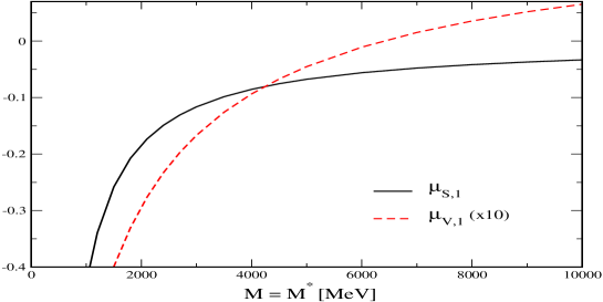
Figure 1: Coefficients $\mu_{S,1}$ and $\mu_{V,1}$ in the magnetic moment operator (54) that are bilinear in the heavy meson wavefunction as functions of the heavy meson masses for $\alpha=0$ in the charm sector, i.e. for ${\cal C}=2/3$.

In figure 1 we show the numerical results for the coefficients $\mu_{S,1}$ and $\mu_{V,1}$ as functions of (equal) heavy meson masses. Obviously these coefficients tend to zero as the mass increases. This behavior is expected from the heavy mass limit since properties, such as the magnetic moments, that are related to spin of the heavy quark are suppressed by inverse powers of the heavy quark mass. Note that also the hyperfine parameter $\chi$ tends to zero in the heavy limit [23] and thus the reduction of $\mu_{S,1}$ implies that of $\tilde{\mu}_{S,1}$. To nevertheless obtain a non–vanishing result in the heavy limit the authors of ref. [32] added an extra term with an undetermined parameter to ${\cal L}_{\rm heavy}$ that is linear in the photon field and thus does only contribute to electromagnetic properties of the heavy baryons [33]. It was argued in ref. [32] that this term would be necessary to describe the radiative decays $Q\to P\gamma$. This term introduces an additional, so far undetermined parameter which may be interpreted as the intrinsic magnetic moment of the heavy meson field. Adopting a canonical value, $1/2M$, leads to $\mu_{\Lambda_{c}}\approx 0.37{\rm n.m.}$ [34], a value considerably larger than our result. It is important to note that the model we consider is capable of describing such radiative decays [29] because it is formulated for finite heavy meson masses rather than in the strict heavy limit. Thus there is no need for any additional photon coupling in our model. The decrease of the $\mu_{S,1}$ and $\mu_{V,1}$ with the increase of the heavy meson mass can also be observed from table 2 where we list these quantities for the physical cases as functions of the undetermined parameter $\alpha$. In this case, of course, the pseudoscalar and vector meson masses are different, cf. eq. (22).

We see that the coefficients $\mu_{S,1}$ and $\mu_{V,1}$ that are bilinear in the heavy meson wavefunctions exhibit quite a pronounced dependence on the undetermined parameter $\alpha$. However, this dependence does not propagate to the magnetic moments of the heavy baryons as seen in tables 3 and 4. One reason is that the total magnetic moments are dominated by $\mu_{S,0}$ and $\mu_{V,0}$, the coefficients that contain only the light mesons profile functions. The other reason is that the combination $\tilde{\mu}_{S,1}=\chi\mu_{S,0}-\mu_{S,1}$ essentially stays constant due to the decrease of $\chi$ with $\alpha$, cf. table 1.

Table 3: Magnetic moments of heavy baryons in the charm sector given in units of nuclear magnetons [n.m.]

$\alpha$	${\quad\Lambda_{C}\quad}$	${\quad\Sigma_{C}^{++}\quad}$	${\quad\Sigma_{C}^{+}\quad}$	${\quad\Sigma_{C}^{0}\quad}$	${\Sigma_{C}^{+}\rightarrow\Lambda_{C}}$
-0.3	0.12	2.46	0.25	-1.96	-2.26
0	0.12	2.45	0.25	-1.96	-2.26
0.3	0.13	2.45	0.24	-1.96	-2.26
0.6	0.13	2.45	0.24	-1.96	-2.26

Table 4: Magnetic moments of heavy baryons in the bottom sector given in units of nuclear magnetons [n.m.]

$\alpha$	${\quad\Lambda_{B}\quad}$	${\quad\Sigma_{B}^{+}\quad}$	${\quad\Sigma_{B}^{0}\quad}$	${\quad\Sigma_{B}^{-}\quad}$	${\Sigma_{B}^{0}\rightarrow\Lambda_{B}}$
-0.3	-0.02	2.52	0.29	-1.93	-2.24
0	-0.02	2.52	0.29	-1.93	-2.24
0.3	-0.02	2.52	0.29	-1.94	-2.24
0.6	-0.02	2.52	0.29	-1.94	-2.23

In table 5 we show the results for the magnetic moments obtained in bound state approach to the Skyrme model. For the charm sector these results are the same as those denoted “SET II” in table 7 of ref. [17]. The calculation in the bottom sector is that of the kaon sector with the replacement $M_{\rm K}\to 5279{\rm MeV}$.

Table 5: Magnetic moments (in nuclear magnetons) of heavy baryons using the bound state approach to the Skyrme model [17]. In this model we find $\mu_{p}=1.97{\rm n.m.}$ and $\mu_{n}=-1.24{\rm n.m.}$.

	${\quad\Lambda_{Q}\quad}$	${\quad\Sigma_{Q}^{I_{3}=1}\quad}$	${\quad\Sigma_{Q}^{I_{3}=0}\quad}$	${\quad\Sigma_{Q}^{I_{3}=-1}\quad}$	${\Sigma_{Q}^{I_{3}=0}\rightarrow\Lambda_{Q}}$
$Q=C$	0.20	1.96	0.42	-1.12	-1.67
$Q=B$	-0.21	2.22	0.56	-1.11	-1.54

Besides the lower scale for the magnetic moments of the light baryons, the essential difference is that the contribution of the heavy meson bound states to the magnetic moments does not decrease as the heavy meson mass increases. Of course, that is expected, as the model of ref. [17] does not reflect the heavy quark spin symmetry.

We finally would like to compare our predictions with those of other descriptions for heavy baryons. Analyses of QCD spectral sum rules yield [35]: $\mu_{\Lambda_{c}}=(0.15\pm 0.05){\rm n.m.}$, $\mu_{\Sigma_{c}^{++}}=(2.1\pm 0.3){\rm n.m.}$, $\mu_{\Sigma_{c}^{+}}=(0.23\pm 0.03){\rm n.m.}$, and $\mu_{\Sigma_{c}^{0}}=(-1.6\pm 0.2){\rm n.m.}$. These values agree nicely with our results. On the other hand, this result for the magnetic moment of $\Lambda_{c}$ is smaller than the one obtained from assuming a canonical intrinsic magnetic moment of the heavy meson fields [34]. In our approach those four magnetic moments ($\mu_{\Lambda_{c}}$, $\mu_{\Sigma_{c}^{++}}$, $\mu_{\Sigma_{c}^{+}}$ and $\mu_{\Sigma_{c}^{0}}$) contain the isoscalar piece $\mu_{{\Sigma}_{Q}^{I_{3}=0}}$ which is dominated by the light meson isoscalar contribution, $\mu_{S,0}$. We therefore compare our results for the transition magnetic moments, $\mu_{{\Sigma}_{Q}^{I_{3}=0}\to\Lambda_{Q}}$ which do not contain $\mu_{{\Sigma}_{Q}^{I_{3}=0}}$, to results from light cone QCD sum rules [36]: $\mu_{{\Sigma}_{C}\to\Lambda_{C}}=-(1.5\pm 0.4){\rm n.m.}$ and $\mu_{{\Sigma}_{B}\to\Lambda_{B}}=-(1.6\pm 0.4){\rm n.m.}$. We find that our predictions are only slightly larger (in magnitude), in addition, those sum rule results have sizable error bars.

5 Summary

In this study we have employed the bound state approach to compute magnetic moments of heavy baryons with a single heavy quark. In this approach the heavy baryon is constructed from a heavy meson field that is bound in the background field of a light baryon. The latter emerges as a soliton of light meson fields. In the model, that we consider here, this soliton contains both light pseudoscalar and light vector meson fields. This extension of the original Skyrme model is known to reasonably describe the phenomenology of light baryons. This is particularly the case for the magnetic moments of proton and neutron. For the heavy sector we have adopted a relativistic Lagrangian which does not directly reflect the heavy quark symmetry. Rather this model embodies the physical values of the heavy meson masses. However, in the limit of infinitely large heavy meson masses it properly reflects the heavy spin flavor symmetry. We have then introduced and canonically quantized the collective coordinates that parameterize the spin–flavor orientation of the soliton and the bound state wavefunction to generate baryon states.

We have extracted the operator of the electromagnetic current from the electromagnetically gauged action. To compute baryon magnetic moments we have sandwiched the appropriate combination of this operator between baryon states. For the magnetic moments of the heavy baryons experimental data do not yet exist, thus we have compared our results with to predictions of other models. Specifically, results are available for spectral sum rule and QCD light cone sum rule analyses. Although our prediction for the transition magnetic moments, $\mu_{{\Sigma}_{Q}^{I_{3}=0}\to\Lambda_{Q}}$ is slightly larger than in the QCD sum rule approach, the overall picture is that the predictions in these two descriptions for heavy baryon properties are very similar. On the other hand, we have seen that the bound state approach to the $SU_{F}(N)$ Skyrme model, which does not respect the heavy spin flavor symmetry, gives significantly different predictions to the magnetic moments of heavy baryons with a single quark. Not surprisingly, these differences are quite distinct for the magnetic moment of $\Lambda_{Q}$ which is most sensitive to the heavy quark contribution to the magnetic moments.

Appendix

In this appendix we list the explicit expressions for the functionals of various meson profiles that parameterize the collective coordinate Lagrangian (43). These functionals have already been reported in the literature [26, 14, 23]. However, because notations do vary within those papers, we list them here for completeness.

First we focus on quantities that only involve the light pseudoscalar and light vector meson profiles, cf. eq. (16). The classical mass is given by

$$M_{\rm cl} = 4\pi\int dr\left\{\frac{f_{\pi}^{2}}{2}(F^{\prime 2}r^{2}+2\sin{F})+m_{\pi}^{2}f_{\pi}^{2}\left(1-\cos{F}\right)\right.$$ (77)

$$\hskip 42.67912pt-\frac{r^{2}}{2g^{2}}(\omega^{\prime 2}+m_{V}^{2}\omega^{2})+\frac{1}{g^{2}}[G^{\prime 2}+\frac{G^{2}}{2r^{2}}(G+2)^{2}]$$

$$\hskip 42.67912pt+\frac{m_{V}^{2}}{g^{2}}(1+G-\cos{F})^{2}+\frac{\gamma_{1}}{g}F^{\prime}\omega\sin^{2}{F}-\frac{2\gamma_{2}}{g}G^{\prime}\omega\sin{F}$$

$$\hskip 42.67912pt\left.+\frac{\gamma_{3}}{g}F^{\prime}\omega G(G+2)+\frac{1}{g}\left(\gamma_{2}+\gamma_{3}\right)F^{\prime}\omega\left[1-2(G+1)\cos{F}+\cos^{2}{F}\right]\right\}\,.$$

Its variation gives the soliton profiles $F$, $G$ and $\omega$. The moment of inertia reads

$$\alpha^{2} = \frac{8\pi}{3}\int dr\Big{\{}f_{\pi}^{2}r^{2}\sin^{2}{F}-\frac{4}{g^{2}}(\varphi^{\prime 2}+2\frac{\varphi^{2}}{r^{2}}+m_{V}^{2}\varphi^{2})+\frac{m_{V}^{2}}{2g^{2}}r^{2}[(\xi_{1}+\xi_{2})^{2}+2(\xi_{1}-1+\cos{F})^{2}]$$ (82)

$$\hskip 42.67912pt+\frac{1}{2g^{2}}[(3\xi_{1}^{\prime 2}+2\xi_{1}^{\prime}\xi_{2}^{\prime}+\xi_{2}^{\prime 2})r^{2}+2(G^{2}+2G+2)\xi_{2}^{2}+4G^{2}(\xi_{1}^{2}+\xi_{1}\xi_{2}-2\xi_{1}-\xi_{2}+1)]$$

$$\hskip 42.67912pt+\frac{4}{g}\gamma_{1}\varphi F^{\prime}\sin^{2}{F}+\frac{4}{g}\gamma_{3}\varphi F^{\prime}[(G-\xi_{1})(1-\cos{F})+(1-\cos{F})^{2}-G\xi_{1}]$$

$$\hskip 42.67912pt+\frac{2\gamma_{2}}{g}\left[\varphi^{\prime}\sin{F}(G-\xi_{1}+2-2\cos{F})+\varphi\sin{F}(\xi_{1}^{\prime}-G^{\prime})\right.$$

$$\hskip 42.67912pt\left.+\varphi F^{\prime}\left(2+2\sin^{2}{F}+(\xi_{1}-G-2)\cos{F}-2(\xi_{1}+\xi_{2})\right)\right]\Big{\}}\,.$$

Again, by variation the profile functions $\xi_{1}$, $\xi_{2}$ and $\varphi$ are obtained. The classical profile functions serve as source fields.

The quantities $I_{\epsilon}$ and $\chi$ are additionally functionals of the heavy meson fields. For the bound state in the P–wave channel one obtains upon substitution of the ansatz (36)

$$I_{\epsilon} = \int drr^{2}\Bigg{(}\Phi^{\prime 2}+\left[M^{2}-\left(\epsilon-\frac{\alpha}{2}\omega\right)^{2}+\frac{2}{r^{2}}\left(1+\frac{1}{2}R_{\alpha}\right)^{2}\right]\Phi^{2}+M^{*2}\left[\Psi_{1}^{2}+\frac{1}{2}\Psi_{2}^{2}-\Psi_{0}^{2}\right]$$ (83)

$$+\frac{1}{2}\left[\Psi_{2}^{\prime}-\frac{1}{r}\Psi_{2}\right]^{2}+\frac{1}{r}R_{\alpha}\Psi_{1}\Psi_{2}^{\prime}+\frac{1}{r^{2}}R_{\alpha}\left(\Psi_{1}+\Psi_{2}\right)\Psi_{2}+\frac{1}{2r^{2}}R_{\alpha}^{2}\left(\Psi_{1}^{2}+\frac{1}{2}\Psi_{2}^{2}\right)$$

$$-\left[\Psi_{0}^{\prime}-\left(\epsilon-\frac{\alpha}{2}\omega\right)\Psi_{1}\right]^{2}-\frac{1}{2}\left[\frac{R_{\alpha}}{r}\Psi_{0}+\left(\epsilon-\frac{\alpha}{2}\omega\right)\Psi_{2}\right]^{2}$$

$$-d\Bigg{\{}\frac{2}{r}{\rm sin}F\left[\Psi_{2}\Psi_{0}^{\prime}-\frac{R_{\alpha}}{r}\Psi_{0}\Psi_{1}-\left(\epsilon-\frac{\alpha}{2}\omega\right)\Psi_{1}\Psi_{2}\right]$$

$$\hskip 28.45274pt+\frac{F^{\prime}}{r}\left[\frac{r}{2}\left(\epsilon-\frac{\alpha}{2}\omega\right)\Psi_{2}^{2}-\left(1-{\rm cos}F\right)\Psi_{0}\Psi_{2}\right]\Bigg{\}}+2Md\left[F^{\prime}\Psi_{1}-\frac{{\rm sin}F}{r}\Psi_{2}\right]\Phi$$

$$+\frac{2\sqrt{2}cM}{gm_{V}}\left[2\omega^{\prime}\Psi_{0}\Psi_{1}-\frac{2G^{\prime}}{r}\Psi_{1}\Psi_{2}+\frac{G}{2r^{2}}\left(G+2\right)\Psi_{2}^{2}\right]$$

$$-\frac{4\sqrt{2}c}{gm_{V}}\Bigg{\{}\frac{1}{r^{2}}\left(\epsilon-\frac{\alpha}{2}\omega\right)\left[G\left(G+2\right)\Psi_{1}-rG^{\prime}\Psi_{2}\right]\Phi-\frac{\omega^{\prime}}{r}\left[1+\frac{R_{\alpha}}{2}\right]\Psi_{2}$$

$$\hskip 56.9055pt+\frac{1}{r^{2}}\left[G\left(G+2\right)\Phi^{\prime}+G^{\prime}\left(2+R_{\alpha}\right)\Phi\right]\Psi_{0}\Bigg{\}}\Bigg{)}\,.$$

Here a prime indicates a derivative with respect to the radial coordinate $r$. Furthermore the abbreviation $R_{\alpha}={\rm cos}F-1+\alpha\left(1+G-{\rm cos}F\right)$ has again been used. The functional $I_{\epsilon}$ leads to the equations of motion for the profile functions $\Phi$, $\Psi_{0}$, $\Psi_{1}$, and $\Psi_{2}$ of the fluctuating heavy meson fields. In these equations the classical fields generate the binding potential. The solution to these equations provides the bound state energy, $\epsilon$ and the bound state wavefunctions that are subsequently normalized according to eq. (38).

Finally, we present the explicit expressions for the hyperfine splitting parameter for the bound state in the $P$–wave, cf. section 4. For convenience we employ additional abbreviations with regard to the light meson profiles defined in eqs (16) and (41)

$$V_{1} = {\rm cos}F-\alpha\left(\xi_{1}-1+{\rm cos}F\right)\ ,$$

$$V_{2} = 1-\alpha\left(\xi_{1}+\xi_{2}\right)\ .$$

The explicit expression for the P–wave hyperfine parameter, which enters the mass formula for the even parity heavy baryon (50), reads

$$\chi = \frac{2}{3}\int_{0}^{\infty}dr\ r^{2}\ \rho_{\chi}(r)$$ (84)

$$\rho_{\chi}(r) = \left[\left(\epsilon-\frac{\alpha}{2}\omega\right)\left(V_{2}-2V_{1}\right)-\frac{2\alpha}{r^{2}}\left(2+R_{\alpha}\right)\varphi\right]\Phi^{2}$$ (85)

$$+\left(2V_{1}+V_{2}\right)\left[\left(\epsilon-\frac{\alpha}{2}\omega\right)\Psi_{1}-\Psi_{0}^{\prime}\right]\Psi_{1}$$

$$-\frac{1}{2}\left(V_{2}\Psi_{2}+\frac{4\alpha}{r}\varphi\Psi_{0}\right)\left[\left(\epsilon-\frac{\alpha}{2}\omega\right)\Psi_{2}+\frac{R_{\alpha}}{r}\Psi_{0}\right]$$

$$+\frac{2\alpha}{r}\varphi\Psi_{1}\left(\Psi_{2}^{\prime}+\frac{1}{r}\Psi_{2}+\frac{R_{\alpha}}{r}\Psi_{1}\right)-\frac{\alpha}{r^{2}}\left(2+R_{\alpha}\right)\varphi\Psi_{2}^{2}+4Md\ {\rm sin}F\Phi\Psi_{0}$$

$$-\frac{d}{r}\left\{{\rm sin}F\left[\left(2+R_{\alpha}+V_{1}\right)\Psi_{1}\Psi_{2}-\frac{4\alpha}{r}\varphi\Psi_{0}\Psi_{1}\right]+F^{\prime}\left[\frac{r}{4}V_{2}\Psi_{2}^{2}+2\alpha\varphi\Psi_{0}\Psi_{2}\right]\right\}$$

$$-\frac{4\sqrt{2}cM}{gm_{V}}\left\{\left(3\xi_{1}^{\prime}+\xi_{2}^{\prime}\right)\Psi_{0}\Psi_{1}+\frac{G}{r}\left(2-2\xi_{1}-\xi_{2}\right)\Psi_{0}\Psi_{2}+\frac{2}{r}\varphi^{\prime}\Psi_{1}\Psi_{2}+\frac{1}{r^{2}}\varphi\Psi_{2}^{2}\right\}$$

$$-\frac{4\sqrt{2}c}{gm_{V}}\Bigg{\{}\left(\epsilon-\frac{\alpha}{2}\omega\right)\left(\frac{4}{r^{2}}\varphi\Psi_{1}+\frac{2}{r}\varphi^{\prime}\Psi_{2}\right)\Phi+\left(V_{1}-\frac{V_{2}}{2}\right)\left[\frac{G}{r^{2}}\left(G+2\right)\Psi_{1}-\frac{G^{\prime}}{r}\Psi_{2}\right]\Phi$$

$$+\frac{G}{r^{2}}\left(2+R_{\alpha}\right)\left(2\xi_{1}+\xi_{2}-2\right)\Phi\Psi_{1}+\frac{2}{r^{2}}\left[2\varphi\Phi^{\prime}+\left(2+R_{\alpha}\right)\varphi^{\prime}\Phi-\alpha G^{\prime}\varphi\Phi\right]\Psi_{0}$$

$$-\frac{1}{r}\left[\left(G+2\right)\xi_{2}\Phi^{\prime}+\left(1+\frac{1}{2}R_{\alpha}\right)\left(\xi_{1}^{\prime}+\xi_{2}^{\prime}\right)\Phi-\alpha\omega^{\prime}\varphi\Phi\right]\Psi_{2}\Bigg{\}}\,.$$

Substituting the bound state profiles as well as the soliton yields numerical results which are used to compute the heavy baryon spectrum according to eq. (50).

References

-
[1]
E. Eichten and F. Feinberg,
Phys. Rev. D23 (1981) 2724;
M. B. Voloshin and M. A. Shifman, Yad. Fiz. 45 (1987) 463 (Sov. J. Nucl. Phys. 45 (1987) 292);
N. Isgur and M. B. Wise, Phys. Lett. B232 (1989) 113; B237 (1990) 527;
H. Georgi, Phys. Lett. B240 (1990) 447. -
[2]
E. Jenkins and A. V. Manohar,
Phys. Lett. B294 (1992) 273;
Z. Guralnik, M. Luke, and A. V. Manohar, Nucl. Phys. B390 (1993) 474;
E. Jenkins, A. V. Manohar, and M. B. Wise, Nucl. Phys. B396 (1993) 27; ibid. 38. -
[3]
M. Rho, in
Baryons as Skyrme Solitons, World Scientific, 1994,
edited by G. Holzwarth, page 183, arXiv:hep-ph/9210268.
D. P. Min, Y. Oh, B. Y Park, and M. Rho, hep-ph/9209275;
H. K. Lee, M. A. Novak, M. Rho, and I. Zahed, Ann. Phys. (N.Y.) 227 (1993) 175;
M. A. Novak, M. Rho, and I. Zahed, Phys. Lett. B303 (1993) 130.
D. P. Min, Y. Oh, B. Y Park, and M. Rho, Intl. J. Mod. Phys. E4 (1995) 47;
L. P. Gamberg, H. Weigel, U. Zuckert, and H. Reinhardt, Phys. Rev. D54 (1996) 5812;
M. Harada, F. Sannino, J. Schechter, and H. Weigel, Phys. Rev. D56 (1997) 4098 - [4] K. S. Gupta, M. A. Momen, J. Schechter, and A. Subbaraman, Phys. Rev. D47 (1993) R4835.
- [5] M. A. Momen, J. Schechter, and A. Subbaraman, Phys. Rev. D49 (1994) 5970.
- [6] Y. Oh, B. Y. Park, and D. P Min, Phys. Rev. D49 (1994) 4649.
- [7] Y. Oh, B. Y. Park, and D. P Min, Phys. Rev. D50 (1994) 3350.
- [8] G. t’ Hooft, Nucl. Phys. B72 (1974) 461; B75 (1975) 461.
- [9] E. Witten, Nucl. Phys. B160 (1979) 57.
-
[10]
G. Holzwarth and B. Schwesinger,
Rep. Prog. Phys. 49 (1986) 825;
I. Zahed and G. E. Brown, Phys. Rep. 142 (1986) 1. - [11] Ulf-G. Meißner, Phys. Rep. 161 (1988) 213.
- [12] B. Schwesinger, H. Weigel, G. Holzwarth, and A. Hayashi, Phys. Rep. 173 (1989) 173.
-
[13]
R. Alkofer, H. Reinhardt, and H. Weigel,
Phys. Rep. 265 (1996) 139;
C. Christov et al., Prog. Part. Nucl. Phys. 37 (1996) 91. - [14] H. Weigel, Intl. J. Mod. Phys. A11 (1996) 2419.
-
[15]
C. Callan and I. Klebanov,
Nucl. Phys. B262 (1985) 365;
C. Callan, K. Hornbostel, and I. Klebanov, Phys. Lett. B202 (1988) 269;
K. M. Westerberg and I. Klebanov, Phys. Rev. D50 (1994) 5834. - [16] J. Kunz and P.J. Mulders, Phys. Lett. B231 (1989) 335.
- [17] Y.S. Oh, D.P. Min, M. Rho, and N.N. Scoccola, Nucl. Phys. A534 (1991) 493.
-
[18]
J. Blaizot, M. Rho, and N. Scoccola,
Phys. Lett. B209 (1988) 27;
N. Scoccola, H. Nadeau, M. A. Novak, and M. Rho, Phys. Lett. B201 (1988) 425;
D. Kaplan and I. Klebanov, Nucl. Phys. B335 (1990) 45;
Y. Kondo, S. Saito, and T. Otofuji, Phys. Lett. B256 (1991) 316;
M. Rho, D. O. Riska, and N. Scoccola, Z. Phys. A341 (1992) 343;
H. Weigel, R. Alkofer, and H. Reinhardt, Nucl. Phys. A576 (1994) 477. - [19] Z. Aziza Baccouche, C.K. Chow, T.D. Cohen, and B.A. Gelman, Phys. Lett. B514 (2001) 346
- [20] P. Jain et. al, Phys. Rev. D40 (1989) 855.
- [21] R. Johnson et. al, Phys. Rev. D42 (1990) 2998
- [22] J. Schechter and A. Subbaraman, Phys. Rev. D48 (1993) 332.
-
[23]
J. Schechter, A. Subbaraman, S. Vaidya, and H. Weigel,
Nucl. Phys. A590 (1995) 655;
E: Nucl. Phys. A598 (1996) 583;
M. Harada et. al, Nucl. Phys. A625 (1997) 789; Phys. Lett. B390 (1997) 329; - [24] H. Weigel and S. Scholl, AIP Conf. Proc. 687 (2003) 62.
- [25] P. Jain et. al, Phys. Rev. D37 (1988) 3252.
- [26] Ulf-G. Meißner, N. Kaiser, H. Weigel, and J. Schechter, Phys. Rev. D39 (1989) 1956.
-
[27]
T.H. Skyrme, Proc. Roy. Soc. Lond. A260 (1961) 127;
G.S. Adkins, C.R. Nappi, and E. Witten, Nucl. Phys. B228 (1983) 552. - [28] Ö. Kaymakcalan, S. Rajeev, and J. Schechter, Phys. Rev. D30 (1984) 594.
- [29] P. Jain, A. Momen, and J. Schechter, Int. J. Mod. Phys. A10 (1995) 2467.
- [30] N.W. Park and H. Weigel, Nucl. Phys. A541 (1992) 453.
- [31] K. Hagiwara et al., [Particle Data Group Collaboration], Phys. Rev. D66 (2002) 010001.
- [32] Y. Oh and B. Y. Park, Mod. Phys. Lett. A11 (1996) 653.
-
[33]
H.Y. Cheng et al.,
Phys. Rev. D 47 (1993) 1030;
P.L. Cho and H. Georgi, Phys. Lett. B 296 (1992) 408 [Erratum-ibid. B 300 (1993) 410];
J.F. Amundson et al., Phys. Lett. B 296 (1992) 415. - [34] M.J. Savage, Phys. Lett. B 326 (1994) 303.
- [35] S. L. Zhu, W. Y. Hwang, and Z. S. Yang, Phys. Rev. D56 (1997) 7273.
- [36] T. M. Aliev, A. Ozpineci, and M. Savci, Phys. Rev. D65 (2002) 096004.