Phenomenology of a 5D Orbifold $SU(3)_{W}$ Unification model

Abstract

We study the phenomenology of a 5D $SU(3)_{W}$ model on a $S_{1}/(Z_{2}\times Z^{\prime}_{2})$ orbifold in which the minimal scalar sector plays an essential role of radiatively generating neutrino Majorana masses without the benefits of right-handed singlets. We carefully examine how do the exotic scalars affect the renormalization group (RG) equations for the gauge couplings and the 5D $SU(3)_{W}$ unification. We found that the compactification scale of extra dimension is in the range of $1/R\sim 1.5-5$ TeV. The possibility of the existence of relatively low mass Kaluza-Klein excitations makes the phenomenology of near term interest. Some possible bilepton signatures can be searched for in future colliders and in neutrino scattering experiments with intense neutrino beams. The low energy constraints from muon physics and lepton number violating decay process induced by bilepton are also discussed. These constraints can provide new information on the structure of Yukawa couplings which might be useful for future model building.

I Introduction

In 1971, an electroweak that unifies the $SU(2)\times U(1)$ symmetry of the standard model(SM) into $SU(3)_{W}$ was suggested Weinberg:1971nd . Here each family of the SM leptons is grouped to form a $SU(3)_{W}$ fundamental representation which is akin to the forgotten Konopinski-Mahmoud Konopinski:1953gq assignments. The model predicts the weak mixing angle to be $\sin^{2}\theta_{\rm W}=0.25$ at the tree level. This is tantalizingly close to the measured value of $\sin^{2}\theta_{\rm W}=0.2311$. Although the prediction is appealing, it was soon abandoned because the insurmountable theoretical difficulty to embed the quarks into any $SU(3)_{W}$ multiplet. Another relevant attempt suggested by 331model is the so called 3-3-1 model. In this model, the gauge group is extended to $SU(3)_{c}\times SU(3)_{W}\times U(1)$ such that the quarks can be embedded into it. This unification came with a hefty price. Firstly, three extra exotic quarks were introduced to complete the $SU(3)_{W}$ multiplets. Secondly, the scalar potential which consists of three triplets and one sextet had to be fine tuned to get the symmetry breaking pattern right. Finally, the third family quarks had to be put in a representation which is different from the first two generations.

Recently, the development of orbifold grand unified theory(GUT) models in the extra dimension brane world scenario has opened up a new direction for model building. The old $SU(3)_{W}$ idea was revived by several groups orbifold_SU3 by promoting it to a five dimensional (5D) model. The $SU(3)_{W}$ is a gauge symmetry in the full 5D bulk space. It is broken to the SM electroweak $SU(2)_{L}\times U(1)_{Y}$ by suitable choice of orbifold parities. Then the $SU(2)_{L}\times U(1)_{Y}$ symmetry is further reduced to $U(1)_{\rm EM}$ via the usual Higgs mechanism. In such a construction, the tree-level prediction of $\sin^{2}\theta_{\rm W}=1/4$ is preserved and the quarks can be placed at the orbifold fixed point where only the SM symmetry manifests; thus avoiding the long standing quark embedding problem. Clearly a dichotomy between quarks and leptons still exists but it is no longer inconsistent. A closer look at the Yukawa sector requires at least one bulk scalar in ${\bf 3}$ representation and one more bulk scalar in the symmetrical ${\bf\bar{6}}$ representation to give viable charged lepton mass pattern. As a result, the electroweak symmetry breaking pattern is controlled by the vacuum expected values(VEVs) of these two bulk scalars.

Meanwhile there are new developments in the area of experimental neutrino physics. There is now strong evidence for neutrino oscillations and nonzero neutrino masses provided recently by many experiments SuperK ; SNO ; KamL ; WMAP which clearly demands new physics beyond the SM for their explanation. The most popular suggestion for giving the active neutrino masses is the seesaw mechanism in GUTs in which one right-handed SM singlet fermion with a mass around GUT scale per SM family is introduced. Each right-handed singlet either belong to the fundamental representation, like in $SO(10)$ GUT, or be put in by hand as in $SU(5)$ GUT. Usually, extra family symmetry is required to obtain neutrino masses and mixing angles that are in accord with the known experimental measurements. In extra dimensional models with right-handed bulk singlet(s), the small four dimensional ( 4D ) effective Dirac masses can be a natural outcome of large extra dimension volume dilution effect. Compared to bulk neutrino model, in a 4D model, the neutrino masses can still emerge by incorporating the right-handed singlet(s) but extreme fine tuning is required. Both of above mentioned methods require a right-handed singlet going into action. An alternative way to give light neutrino masses is through 1-loop quantum corrections. The prototype model was constructed some time agoZee in which the presence of a $SU(2)$ singlet as the lepton number violating source is crucial. The early version of this kind of model gives at most the bi-maximal mixing angle which is ruled out by the latest SNO data. At the expense of introducing more exotic Higgs fields this kind of models can be made to agree with observation again. However, all these constructions suffer from being ad hoc.

Simultaneously confronting $\sin^{2}\theta_{W}$ problem and recent neutrino data, we investigated a radiative mechanism for neutrino mass based on 5D orbifold $SU(3)_{W}$ GUT SU3:triumf . We found that it is possible to accommodate large mixing angle MSW solution to the neutrino data with a minimum scalar sector, in the sense that the charged lepton mass hierarchy can be accounted for, without much fine tuning of parameters. This idea is further pursued by us and has been extended to 5D non-supersymmetric $SU(5)$ model SU5:TRIUMF . But due to the high compactification scale, $1/R>10^{14}$ GeV, the $SU(5)$ version is phenomenologically less interesting . The non-supersymmetric $SU(3)_{W}$ model on the other hand implies a large extra dimension with the compactification scale, $1/R$, in the range of $1.5-5$ TeV. Thus, the stability problem of the Higgs sector is not as severe as many other theories. This point also justifies why the supersymmetry need not be introduced in this model. The theoretical consistency, see the discussion in section III, sets a upper bound on $1/R$ to be around $5$ TeV with the actual value depending weakly on a few free parameters. Obviously, the low value of $1/R$ makes it interesting for colliders and low energy physics tests of the validity of the model are meaningful. Interestingly, all the new physics effects appear mainly in the lepton sectors which makes it distinguishable from other GUT models. For a brief review of these models see JR .

The purpose of this paper is to carefully consider the phenomenological consequences of the 5D $SU(3)_{W}$ GUT. Nontrivial result already can be drawn from analyzing renormalization group equations (RGEs) and unification altered by the extended scalar sector.

The characteristic phenomenology of $SU(3)_{W}$ GUT arises from the presence of vector or scalar bileptons. There exists many phenomenology surveys on the general bilepton case Cuypers ; bilepton_gen . Also there are studies that focused either on the 3-3-1 model 331pheno ; Dion:1998pw or other GUTs bilepton_GUT . The presence of Kaluza-Klein ( KK ) excitations of bileptons or SM gauge bosons in this 5D $SU(3)_{W}$ model makes our study very different from the existing analysis. The KK excitations will affect the effective gauge and Yukawa couplings. Signatures in high energy collider experiments can come from direct production of new particles if they are light enough. They can also come from modification of the expected SM signature. Depending on the mixings which can occur among the vector bileptons and also the leptons, we found the deviation of angular distributions from SM expectations can be as high as few tens percent in the Bhabha and Møller scatterings which could be probed by the future linear colliders. Also, in low energy neutrino scattering the KK excitations play a role.

Current low energy leptonic experiment such as rare muon processes already impose many constraints on this model, especially on the Yukawa sector as we will show.

Here is our plan for the paper. In the next section, we give necessary details of the 5D orbifold $SU(3)_{W}$ model. The coupling of the bilepton gauge bosons to leptons will be spelled out explicitly. The RGEs for the gauge couplings are examined in section III. This is done in greater detail than available in the literature. Then the tree-level decay widths of KK excitations are given in section IV. The low energy constraint will be discussed in section V, where muon decay, muonium-antimuonium transition, and lepton flavor violating processes are discussed. Section VI is devoted to the study of collider signatures, focusing on the Bhabha and Møller scatterings. Also, we comment on the possible bilepton direct production in various colliders. The low energy neutrino electron scattering receives correction from the KK excitations of SM gauge bosons and the vector bileptons. This will be discussed in section VII. We give the conclusion at section VIII. Some handy formulas are collected in the Appendix.

II The 5D orbifold $SU(3)_{W}$ model

The $SU(3)_{W}$ unification model is defined on the orbifold $M_{4}\times S_{1}/(Z_{2}\times Z^{\prime}_{2})$ with the 4D Minkowski space $M_{4}$ coordinates denoted by $x^{\mu}(\mu=0,1,2,3)$ and the extra spatial dimension by $y$. The latter is compactified into a circle $S_{1}$ of radius $R$, or $y=[-\pi R,\pi R]$, and is orbifolded by a $Z_{2}$ which identifies points $y$ and $-y$. The resulting space is further divided by a second $Z_{2}^{\prime}$ acting on $y^{\prime}=y-\pi R/2$ to give the final geometry. Therefore, two parity eigenvalues, plus or minus one, can be assigned to the bulk fields under the transformations $P:y\leftrightarrow-y$ and $P^{\prime}:y^{\prime}\leftrightarrow-y^{\prime}$.

The SM lepton left-handed doublet and the right-handed singlet in each family can be embedded into the $SU(3)_{W}$ fundamental representation as

$$L=\left(\begin{array}[]{c}e\\ \nu\\ e^{c}\end{array}\right)_{\mathrm{L}}.$$ (1)

In our convention, $T_{3}=-\lambda_{3}/2$ and $Y=-\sqrt{3}\lambda_{8}/2$ in terms of the standard Gell-Man matrices and ${\mathrm{L}}=(1-\gamma_{5})/2$. The $SU(3)_{W}$ gauge bosons are bulk fields and the 5D field strength is given by

$$G_{MN}=\partial_{M}{\cal A}_{N}-\partial_{N}{\cal A}_{M}-{i\tilde{g}\over\sqrt{M^{*}}}[{\cal A}_{M},{\cal A}_{N}]$$ (2)

with gauge matrix ${\cal A}_{M}=\sum_{a=1}^{8}A^{a}_{M}T^{a}$, the generator $T^{a}=\frac{1}{2}\lambda^{a}$ and $M,N=\{\mu,y\}$. It’s more convenient to express the gauge matrix ${\cal A}_{M}$ in gauge boson’s mass basis:

$${\cal A}_{M}={1\over\sqrt{2}}\left(\begin{array}[]{ccc}0&W^{-}_{M}&U^{-2}_{M}\\ W^{+}_{M}&0&V^{-}_{M}\\ U^{+2}_{M}&V^{+}_{M}&0\end{array}\right)$$ (6)

$$+{Z_{M}\over c_{W}}\left(\begin{array}[]{ccc}{c_{W}^{2}-s_{W}^{2}\over 2}&0&0\\ 0&-\frac{1}{2}&0\\ 0&0&s_{W}^{2}\end{array}\right)+A_{M}\left(\begin{array}[]{ccc}s_{W}&0&0\\ 0&0&0\\ 0&0&-s_{W}\end{array}\right)$$ (13)

where

$$\left(\begin{array}[]{c}Z_{M}\\ A_{M}\end{array}\right)=\left(\begin{array}[]{cc}c_{W}&-s_{W}\\ s_{W}&c_{W}\end{array}\right)\left(\begin{array}[]{c}A^{3}_{M}\\ A^{8}_{M}\end{array}\right)$$ (14)

and $\tilde{e}=\tilde{g}\sin\theta_{W}$. The key to orbifold symmetry breaking is that the individual components of a gauge multiplet need not share the same $(P,P^{\prime})$ parities. It is only required that the all the assignments to bulk fields are consistent with group theory and $P,P^{\prime}$ which are inner automorphisms of $SU(3)_{W}$. The parity matrices ${\rm P}=diag\{+++\}$ and ${\rm P}^{\prime}=diag\{++-\}$ and the parity of $SU(3)_{W}$ gauge fields

$${\cal A}_{\mu}(y)={\rm P}{\cal A}_{\mu}(-y){\rm P}^{-1}\,, {\cal A}_{\mu}(y^{\prime})={\rm P}^{\prime}{\cal A}_{5}(-y^{\prime}){\rm P}^{\prime-1}$$

$${\cal A}_{5}(y)=-{\rm P}{\cal A}_{\mu}(-y){\rm P}^{-1}\,, {\cal A}_{5}(y^{\prime})={\rm P}^{\prime}{\cal A}_{5}(-y^{\prime}){\rm P}^{\prime-1}$$ (15)

are chosen to break the bulk $SU(3)_{W}$ symmetry into $SU(2)\times U(1)$. Then the $(Z_{2},Z^{\prime}_{2})$ parities of the SM gauge bosons and $SU(3)_{W}/(SU(2)\times U(1))$ gauge bosons denoted by $U^{\pm 2},V^{\pm}$, are $(++)$ and $(+-)$ respectively. In other words, only SM gauge bosons have zero modes. Both the $U,V$ gauge bosons and all the $y-$components are heavy KK excitations. Note that the KK modes of the fifth components of gauge bosons are real scalars.

The $SU(3)_{W}$ symmetry is explicitly broken to $SU(2)_{L}\times U(1)$ at the $y=\pi R/2$ fixed point, where the 4D quarks field are forced to live on it. On the other hand, the lepton fields can be placed anywhere in the bulk or on either two fixed points. We choose to put the 4D lepton triplets at $y=0$ which is a $SU(3)_{W}$ symmetric fixed point so that they enjoy the $SU(3)_{W}$ symmetry. This also avoids possible proton decay contact interactions.

As mentioned before, one Higgs triplet $\mathbf{3}$ plus one Higgs anti-sextet $\bar{\mathbf{6}}$ , denoted as $\phi_{6}$, is the minimal scalar set to give viable charged fermion masses (see SU3:triumf ). The parity of scalar fields are chosen to be

$$\phi_{3}(y)={\rm P}\phi_{3}(-y)\,, \phi_{3}(y^{\prime})={\rm P}^{\prime}\phi_{3}(-y^{\prime})$$

$$\phi_{6}(y)={\rm P}\phi_{6}(-y){\rm P}^{-1}\,, \phi_{6}(y^{\prime})=-{\rm P}^{\prime}\phi_{6}(-y^{\prime}){\rm P}^{\prime-1}.$$ (16)

This will allow the appropriate neutral fields to develop VEVs and also avoids tree-level neutrino masses. Another Higgs triplet $\mathbf{3^{\prime}}$ with parities $(+-)$ is introduced to transmit lepton number violation essential for generating Majorana neutrino mass through 1-loop diagrams SU3:triumf . This comes from a triple Higgs interaction of the type of ${\mathbf{3}^{\prime}}^{T}\bar{{\mathbf{6}}}{\mathbf{3}}$ which is consistent with the symmetry of the background geometry.

Now we have all the ingredients to write down explicitly the 5D Lagrangian density

$${\cal L}_{5} = -\frac{1}{2}\mbox{\sl{Tr}}[G_{MN}G^{MN}]+\mbox{\sl{Tr}}[(D_{M}\phi_{6})^{\dagger}(D^{M}\phi_{6})]$$ (17)

$$+ (D_{M}\phi_{3})^{\dagger}(D^{M}\phi_{3})+(D_{M}\phi^{\prime}_{3})^{\dagger}(D^{M}\phi^{\prime}_{3})$$

$$+ \delta(y)\left[\epsilon_{abc}\frac{f_{ij}^{3}}{\sqrt{M^{*}}}\overline{(L^{a}_{i})^{\mathbf{c}}}L^{b}_{j}\phi_{3}^{c}+\epsilon_{abc}\frac{f_{ij}^{{}^{\prime}3}}{\sqrt{M^{*}}}\overline{(L^{a}_{i})^{\mathbf{c}}}L^{b}_{j}\phi_{3}^{{}^{\prime}c}\right.$$

$$+ \left.\frac{f^{6}_{ij}}{\sqrt{M^{*}}}\overline{(L^{a}_{i})^{\mathbf{c}}}\phi_{6\{ab\}}L^{b}_{j}+\bar{L}i\gamma^{\mu}D_{\mu}L\right]$$

$$- V_{0}(\phi_{6},\phi_{3},\phi^{\prime}_{3})-\frac{m}{\sqrt{M^{*}}}\phi_{3}^{T}\phi_{6}\phi^{\prime}_{3}+H.c.$$

$$+ \mbox{quark sector}.$$

The 5D covariant derivatives are given by

$$D_{M}\phi_{3}=(\partial_{M}-i{\tilde{g}\over\sqrt{M^{*}}}{\cal A}_{M})\phi_{3},$$ (18)

$$D_{M}\phi_{6}=\partial_{M}\phi_{6}-i{\tilde{g}\over\sqrt{M^{*}}}[{\cal A}_{M}\phi_{6}+({\cal A}_{M}\phi_{6})^{T}]\,.$$ (19)

The notations are self explanatory. The cutoff scale $M^{*}$ is introduced to make the coupling constants dimensionless. The quark sector is not relevant now and will be left out. The complicated scalar potential is gauge invariant and orbifold symmetric and will not be specified since it is not needed here. Since we will only concentrate on tree level processes in this paper, the gauge fixing term is not specified here. This can be done either covariantly or non-covariantly GF .

The branching rules of bulk fields and the labels to each components are summarized below:

$$8^{\mu} = \underbrace{(1,0)_{++}}_{B^{\mu}}+\underbrace{(3,0)_{++}}_{A^{\mu}}+\underbrace{(2,-3/2)_{+-}+(2,+3/2)_{+-}}_{(U,V)^{\mu}}$$

$$8^{5} = \underbrace{(1,0)_{-+}}_{B^{5}}+\underbrace{(3,0)_{-+}}_{A^{5}}+\underbrace{(2,-3/2)_{--}+(2,+3/2)_{--}}_{(U,V)^{5}}$$

$$\mathbf{3} = \underbrace{(2,-1/2)_{++}}_{H_{W1}}+\underbrace{(1,1)_{+-}}_{H_{S}}$$

$$\mathbf{3}^{\prime} = \underbrace{(2,-1/2)_{+-}}_{H^{\prime}_{W1}}+\underbrace{(1,1)_{++}}_{H^{\prime}_{S}}$$

$$\mathbf{\bar{6}} = \underbrace{(3,+1)_{+-}}_{H_{T}}+\underbrace{(2,-1/2)_{++}}_{H_{W2}}+\underbrace{(1,-2)_{+-}}_{H_{S2}}$$

where the SM quantum numbers are $(SU(2)_{L},U(1)_{Y})$ and the subscripts label the parities $P,P^{\prime}$. Then it is straightforward to obtain the 4D effective interaction by integrating over $y$. In the following we list some relevant Lagrangian for our phenomenological study.

The 4D effective gauge coupling can be identified as $g_{2}=\frac{\tilde{g}}{\sqrt{2\pi RM^{*}}}$ which gives the following charged current interaction

$${\cal L}_{\rm CC}={g_{2}\over\sqrt{2}}\sum_{n=0}\kappa_{n}\left[\overline{e_{L}}\gamma^{\mu}\nu_{L}W^{-}_{n,\mu}+\overline{e_{L}}\gamma_{\mu}e_{R}^{\mathbf{c}}U^{-2}_{n,\mu}\right.$$

$$\left.+\overline{\nu_{L}}\gamma^{\mu}e^{\mathbf{c}}_{R}V^{-1}_{n,\mu}+H.c.\right]$$ (20)

where $\kappa_{n}=(\sqrt{2})^{1-\delta_{n,0}}$. Similarly, the neutral current interactions are worked out to be

$${\cal L}_{\rm NC}=\sum_{n=0}\kappa_{n}{g_{2}\over\cos\theta}\bar{l}\gamma_{\mu}(g^{l}_{L}P_{L}+g^{l}_{R}P_{R})lZ^{\mu}_{n}$$

$$-\sum_{n=0}\kappa_{n}e(\bar{l}\gamma_{\mu}l)A^{\mu}_{n}+\sum_{n=0}\kappa_{n}{g_{2}\over 2\cos\theta}(\bar{\nu}\gamma_{\mu}P_{L}\nu)Z^{\mu}_{n}\,.$$ (21)

The usual SM relations hold: $e=g_{2}\sin\theta_{W}$, $g^{l}_{L/R}=T_{3}(l_{L/R})-\sin^{2}\theta_{\rm W}Q(l_{L/R})$, and there is no extra neutral current except for the KK modes of the photon and the Z boson. The explicit expression of the Yukawa interactions is given by

$${\cal L}_{\rm Y} = {f^{3}_{ij}\over\sqrt{2\pi RM^{*}}}\sum_{n=0}\kappa_{n}\left[\overline{e^{\mathbf{c}}_{L,i}}\nu_{L,j}H^{+}_{S,n}+\overline{e_{R,i}}e_{L,j}H^{0}_{W1,n}+\overline{e_{R,j}}\nu_{L,i}H^{-}_{W1,n}-(i\Leftrightarrow j)\right]$$ (22)

$$+ {f^{{}^{\prime}3}_{ij}\over\sqrt{2\pi RM^{*}}}\sum_{n=0}\kappa_{n}\left[\overline{e^{\mathbf{c}}_{L,i}}\nu_{L,j}H^{{}^{\prime}+}_{S,n}+\overline{e_{R,i}}e_{L,j}H^{{}^{\prime}0}_{W1,n}+\overline{e_{R,j}}\nu_{L,i}H^{{}^{\prime}-}_{W1,n}-(i\Leftrightarrow j)\right]$$

$$+ {f^{6}_{ij}\over\sqrt{2\pi RM^{*}}}\sum_{n=0}\kappa_{n}\left[\overline{e^{\mathbf{c}}_{L,i}}e_{L,j}H^{+2}_{T,n}+(\overline{e^{\mathbf{c}}_{L,i}}\nu_{L,j}+\overline{\nu^{\mathbf{c}}_{L,i}}e_{L,j})H^{+}_{T,n}+\overline{\nu^{\mathbf{c}}_{L,i}}\nu_{L,j}H^{0}_{T,n}\right.$$

$$+ \left.(\overline{e_{R,i}}e_{L,j}+\overline{e_{L,i}}e_{R,j})H^{0}_{W2,n}+(\overline{e_{R,i}}\nu_{L,j}+\overline{\nu_{L,i}}e_{R,j})H^{-}_{W2,n}+\overline{e_{R,i}}e^{\mathbf{c}}_{R,j}H^{-2}_{S2,n}\right]+H.c.$$

After spontaneously symmetry breaking, the $\mathbf{3}$ and the $\bar{\mathbf{6}}$ acquire non-zero VEVs:

$$<\mathbf{3}>=\frac{v_{3}^{3/2}}{\sqrt{2}}\left(\begin{array}[]{c}0\\ 1\\ 0\end{array}\right),<\mathbf{\bar{6}}>=\frac{v_{6}^{3/2}}{\sqrt{2}}\left(\begin{array}[]{ccc}0&0&{1\over\sqrt{2}}\\ 0&0&0\\ {1\over\sqrt{2}}&0&0\end{array}\right)$$ (23)

which are related to the 4D VEV as

$$v_{0}^{2}=2\pi R(v_{6}^{3}+v_{3}^{3})\sim(250\mbox{GeV})^{2}$$ (24)

The gauge boson masses can be derived to be:

$$M_{Wn}^{2} = M_{W0}^{2}+\frac{4n^{2}}{R^{2}},$$ (25)

$$M_{Zn}^{2} = M_{Z0}^{2}+\frac{4n^{2}}{R^{2}},$$ (26)

$$M_{Vn}^{2} = M_{W0}^{2}+\frac{(2n-1)^{2}}{R^{2}},$$ (27)

$$M_{Un}^{2} = {4M_{W0}^{2}\over 1+v_{3}^{3}/v_{6}^{3}}+\frac{(2n-1)^{2}}{R^{2}}\,.$$ (28)

Unless we specify otherwise, in later numerical estimations we shall ignore the zero mode masses for KK excitations. The two VEVs, $v_{3}$ and $v_{6}$, are free parameters. There is no good reason for them to be very different. For the sake of economy we assume $v_{3}=v_{6}$; this also implies that all flavor information are encoded in the Yukawa couplings.

Denoting $l=(e,\mu,\tau)^{T}$, the charged leptons acquire masses through VEVs as usual with

$$(\overline{l_{R}})^{T}{\cal M}_{l}l_{L}+H.c.$$ (29)

and the mass matrix is given by

$${\cal M}_{l}={v_{0}\over\sqrt{2\pi RM^{*}}}\left(\begin{array}[]{ccc}0&f^{3}_{12}&f^{3}_{13}\\ -f^{3}_{12}&0&f^{3}_{23}\\ -f^{3}_{13}&-f^{3}_{23}&0\end{array}\right)$$ (33)

$$+{v_{0}\over 2\sqrt{\pi RM^{*}}}\left(\begin{array}[]{ccc}f^{6}_{11}&f^{6}_{12}&f^{6}_{13}\\ f^{6}_{12}&f^{6}_{22}&f^{6}_{23}\\ f^{6}_{13}&f^{6}_{23}&f^{6}_{33}\end{array}\right)\,.$$ (37)

The above mass matrix can be diagonalized by a bi-unitary rotation with $\psi_{L/R}=U_{L/R}\psi^{\prime}_{L/R}$ where the fields with prime are weak eigenbasis. In this convention,

$$U_{R}{\cal M}_{l}{\cal M}_{l}^{\dagger}U_{R}^{\dagger}=U_{L}{\cal M}^{\dagger}_{l}{\cal M}_{l}U_{L}^{\dagger}={\cal M}^{2}_{diag}\,.$$ (38)

It is straightforward to modify Feynman rules by incorporating the mixing matrices. For example, the lagrangian of charged current in charged leptons’ mass eigenstate becomes:

$${\cal L}_{\rm CC}=g_{2}\sum_{n=1}\overline{e_{Li}}\gamma^{\mu}P_{L}(U_{L}^{\dagger}U_{R}^{*})_{ij}e^{\mathbf{c}}_{Rj}U^{-2}_{n,\mu}+H.c.$$

$$+g_{2}\sum_{n=1}\overline{\nu_{Li}}\gamma^{\mu}P_{L}(U_{L}^{\dagger}U_{R}^{*})_{ij}e^{\mathbf{c}}_{Rj}V^{-1}_{n,\mu}+H.c.$$ (39)

where the subscripts $L$ and $R$ are kept for book keeping. For later use, we define the mixing matrix

$${\cal U}=U_{L}^{\dagger}U_{R}^{*}$$ (40)

which is a CKM-like unitary matrix. By using the identities in the Appendix, the above expression can be rewritten as

$${\cal L}_{\rm CC} = {g_{2}\over 2}\sum_{n=1}\overline{e_{i}}\gamma^{\mu}[P_{L}{\cal U}-P_{R}{\cal U}^{T}]_{ij}e^{\mathbf{c}}_{j}U^{-2}_{n,\mu}+H.c.$$ (41)

$$+ \frac{g_{2}}{2}\sum_{n=1}\overline{\nu_{i}}\gamma^{\mu}[P_{L}{\cal U}-P_{R}{\cal U}^{T}]_{ij}e^{\mathbf{c}}_{j}V^{-1}_{n,\mu}+H.c.$$

The corresponding Feynman diagrams are shown in Fig.1, note that the $W$ vertex is always flavor diagonal.

Figure 1: Feynman rules for charged current vertices.

For completeness, we present the resulting neutrino overall mass scale. This is calculated to be SU3:triumf

$$\bar{m}_{\nu}\sim{gv_{0}\over 16\pi^{2}M_{W}}{m|f^{{}^{\prime}3}|\over(\pi RM^{*})}{m_{\tau}^{2}\ln(M_{2}^{2}/M_{1}^{2})\over M_{1}^{2}-M_{2}^{2}}$$ (42)

where $M_{1}$ and $M_{2}$ are the masses of $H_{W2}$ in $\mathbf{\bar{6}}$ and $H^{\prime}_{S}$ in $\mathbf{3}^{\prime}$ for the leading contribution.

III The RG running of coupling constants

Below the scale $1/R$ the RG running of the gauge couplings are the same as the 4D field theory. When $\mu\gg 1/R$, the inverse fine structure constants obey the following equation:

$${1\over\alpha_{i}(\mu)}={1\over\alpha_{i}(M_{Z})}-{a_{i}\over 2\pi}\ln{\mu\over M_{Z}}-{a^{H}_{i}\over 2\pi}\ln{\mu\over M_{H}}$$

$$-{\tilde{a}\over 4\pi}(\mu R-\ln 2)+{\tilde{a}_{i}^{e}\over 4\pi}\ln\left({\pi\mu R\over 2}\right)$$ (43)

where the beta function coefficients are denoted generically by $a$ and the subscript $i$ is for either $SU(2)$ or $U(1)$. Those with a tilde on top are from KK modes. Also $\tilde{a}\equiv\tilde{a}^{e}+\tilde{a}^{o}$ where $\tilde{a}_{i}^{e,o}$ is the beta function coefficient from the even(odd)-KK mode. By even(odd) we refer to the component fields with $(Z_{2},Z^{\prime}_{2})$ parity $(++)$ or $(--)$ ( $(+-)$ or $(-+)$ ) and tree level KK masses of $2n/R$ ( $(2n-1)/R$ ). The well known power law running was first noticed by Dienes which can also be understood by summing up KK modes contribution level by level and then applying the Stirling’s approximation SU5:TRIUMF . Note that the coefficient in front of the power law running term, $(\mu R-2)$, is universal for every subgroup and plays no role in determining the point of unification. This is no surprise because when $\mu\gg 1/R$ all the acting particles can be clustered into some kind of GUT multiplets. The effect of even- and odd-components splitting in a GUT multiplet shows up in the last term. As unification is concerned, $\tilde{a}^{e}_{i}$ can be equivalently replaced by $-\tilde{a}^{o}_{i}$. The beta function coefficient $a_{i}$ is determined by the well-known formula:

$$a_{i}=\left[-\frac{11}{3}S^{i}_{2}(G)+\frac{2}{3}S^{i}_{2}(F)+\frac{1}{6}S_{2}^{i}(S)\right]$$ (44)

obtained from gauge boson self-energy corrections. In Eq.(44) the first term comes from the gauge boson loops (G); the second one is from Weyl fermion (F) loops; the last one is due to real scalar (S) loops and for complex scalars this should be doubled. $S_{2}$ are standard group theory factors and they depend on the group representations of the respective particles in the loop. The hypercharge coupling is normalized to the unified gauge coupling as $g_{Y}=g_{GUT}/\sqrt{3}$, and the tree level prediction of $\sin^{2}\theta_{\rm W}=1/4$ follows immediately. The contributions from individual fields and their KK modes are listed below in Table 1.

Sources	Component	$a_{1}$	$a_{2}$	Whole multiplet
$\mathbf{3}(+,\pm)$	$(2,-1/2)_{(+,\pm)}$	$1/18$	$1/6$	$1/6$
	$(1,1)_{(+,\mp)}$	$1/9$	$0$
$\mathbf{\bar{6}}(+,-)$	$(2,-1/2)_{(++)}$	$1/18$	$1/6$	$5/6$
	$(3,1)_{(+-)}$	$1/3$	$2/3$
	$(1,-2)_{(+-)}$	$4/9$	$0$
$8^{\mu}(++)$	$(3,0)_{(++)}$	$0$	$-22/3$	$-11$
	$(1,0)_{(++)}$	$0$	$0$
	$(2,-3/2)_{(+-)}$	$-11/2$	$-11/6$
	$(2,+3/2)_{(+-)}$	$-11/2$	$-11/6$
$L^{i}$	$(1,2,-1/2)_{b}$	$1/9$	$1/3$	$(20/27,4/3)$
$e_{R}^{i}$	$(1,1,-1)_{b}$	$2/9$	$0$
$Q^{i}$	$(3,2,1/6)_{b}$	$1/27$	$1$
$u_{R}^{i}$	$(3,1,2/3)_{b}$	$8/27$	$0$
$d_{R}^{i}$	$(3,1,-1/3)_{b}$	$2/27$	$0$
KK	Even component	$\tilde{a}^{e}_{1}$	$\tilde{a}^{e}_{2}$	$\tilde{a}$
$\mathbf{3}(++)$	$(2,-1/2)$	$1/18$	$1/6$	$1/6$
$\mathbf{3}^{\prime}(+-)$	$(1,1)$	$1/9$	$0$	$1/6$
$\mathbf{\bar{6}}(+-)$	$(2,-1/2)$	$1/18$	$1/6$	$5/6$
$8^{\mu}(++)$	$(3,0)$	$0$	$-22/3$	$-11$
	$(1,0)$	$0$	$0$
$8^{5}(-+)$	$(2,-3/2)$	$1/4$	$1/12$	$1/2$
	$(2,+3/2)$	$1/4$	$1/12$

Table 1: Beta function coefficients form varies particles.

The unification condition can be expressed as

$${1\over\alpha_{1}(M_{Z})}-{1\over\alpha_{2}(M_{Z})}={a_{1}-a_{2}\over 2\pi}\ln{\mu\over M_{G}}$$

$$+{a^{H_{3}}_{1}-a^{H_{3}}_{2}\over 2\pi}\ln{M_{H_{3}}\over M_{G}}+{a^{H_{6}}_{1}-a^{H_{6}}_{2}\over 2\pi}\ln{M_{H_{6}}\over M_{G}}$$

$$-{\tilde{a}_{1}^{e}-\tilde{a}_{2}^{e}\over 4\pi}\ln\left({\pi RM_{G}\over 2}\right)$$ (45)

where $M_{H_{3}}$ and $M_{H_{6}}$ are the zero mode masses for $\mathbf{3}^{\prime}$ and $\mathbf{\bar{6}}$ respectively. Plugging in the numbers, $a=(41/18,-19/6)$ $=3\times(20/27,4/3)$ $+(0,-22/3)+(1/18,1/6)$, $a_{H}^{3}=(1/9,0)$, $a_{H}^{6}=(1/18,1/6)$ and $\tilde{a}^{e}=(13/18,-41/6)$, we have

$${2\pi\over\alpha_{1}(M_{Z})}-{2\pi\over\alpha_{2}(M_{Z})}=-{49\over 9}\ln{M_{Z}\over M_{G}}+{1\over 9}\ln{M_{H_{6}}\over M_{H_{3}}}$$

$$-{34\over 9}\ln\left({\pi RM_{G}\over 2}\right).$$ (46)

Note that the dependence of $M_{H_{3}}$ and $M_{H_{6}}$ is very weak since they appear in a ratio in the above although they are strictly unknown parameters of the model.

The values of the couplings at $M_{Z}$ are very accurately measured and is given by $\alpha^{-1}(M_{Z})=127.934(7)$ and $\sin^{2}\theta_{W}=0.23113(15)$. Using

$$\alpha_{1}={3\alpha\over\cos^{2}\theta_{W}}=0.03049(2),\,\alpha_{2}={\alpha\over\sin^{2}\theta_{W}}=0.03382(2)\,.$$ (47)

Eq.(46) can be further simplified numerically to

$$8.2398=\ln{M_{G}\over(\mbox{GeV})}+{1\over 49}\ln{M_{H_{6}}\over M_{H_{3}}}-{34\over 49}\ln\left({\pi RM_{G}\over 2}\right)$$ (48)

which can be easily solved. Some typical solutions are given in Tab.2. The compactified extra space is large and of order few TeV as advertised earlier. The results agrees with previous estimations orbifold_SU3 . Since we do not expect a large hierarchy in the scalar masses this is fairly robust. Note that upper bound of $1/R$ is determined by the requirement of theory consistency, namely $M_{G}>1/R$.

$M_{H_{6}}/M_{H_{3}}$	$(\pi RM_{G})$	$1/R$ (TeV)
	$\pi$	$5.43$
$0.1$	$10$	$3.81$
	$50$	$2.33$
	$100$	$1.88$
	$200$	$1.52$
	$\pi$	$5.18$
$1.0$	$10$	$3.64$
	$50$	$2.22$
	$100$	$1.80$
	$200$	$1.45$
	$\pi$	$5.07$
$3.0$	$10$	$3.56$
	$50$	$2.17$
	$100$	$1.76$
	$200$	$1.42$
	$\pi$	$4.95$
$10.0$	$10$	$3.47$
	$50$	$2.12$
	$100$	$1.71$
	$200$	$1.39$

Table 2: Some typical solutions of unification.

IV Decays of KK modes

Next, we study the decays of KK excitations and begin with KK photons.

A KK photon can decay into any charged brane fermions and lower charged KK fields if kinematics and KK number selection rules allow it. Firstly, we will discuss the case for it to decay into brane fermions. The process is governed by the effective lagrangian: $\sqrt{2}eA^{\mu}_{n}\bar{f}\gamma_{\mu}f$ which leads to the decay rate

$$\Gamma^{f\bar{f}}_{A}={N_{c}\over 12\pi}(\sqrt{2}eq_{f})^{2}M_{n}\sqrt{1-4y_{f}}(1+2y_{f})$$ (49)

where $y_{f}=m_{f}^{2}/M_{n}^{2}$, $N_{c}$ is the color factor of fermion $f$ and $q_{f}$ is the fermion charge in the unit of electron charge. Compared with $1/R\sim 1.5-5$TeV all fermion masses can be ignored, even that of the t-quark. Summing over the SM charged fermions, the total decay width is

$$\Gamma^{f\bar{f}}_{A} = 3{2\alpha\over 3}M_{n}\left[(-1)^{2}+3\left(\frac{2}{3}\right)^{2}+3\left(-\frac{1}{3}\right)^{2}\right]$$ (50)

$$= {16\alpha\over 3}\frac{2n}{R}\,.$$

Secondly , we check whether a given KK photon can decay into final states with lighter KK modes. For the n-th KK photon, the KK number conservation allows it to decay into a pair of KK $W$ bosons such as $W_{m}W_{n-m}$ with the integer $m<n$ or into two channels with $U,V$ final states, see appendix for details. But one of the $U,V$ channel is forbidden by kinematics. At this stage, we do not need to consider KK masses splitting due to quantum corrections except to note that they are small. The tree level masses relation predicts that $M^{A}_{n}\sim M^{U}_{m}+M^{U}_{n-m+1}$ for the decay of $A_{n}\rightarrow U^{\pm 2}_{m}+U^{\mp 2}_{n-m+1}$. The phase space of this process is fully saturated and leave no room for it to happen. Similar consideration applies to any lower KK number final states at tree level. We conclude that decays of all KK excitations are dominated by the final states with brane fermions. So the decay widths are the standard ones times two, due to $\sqrt{2}$ factor in the couplings, with the masses substituted by KK masses:

$$\Gamma_{W}^{(n)} = {(\sqrt{2}g_{2})^{2}M_{Wn}\over 48\pi}(3+3\sum_{ij}|V_{ij}|^{2})$$ (51)

$$= {2\alpha\over s_{W}^{2}}\frac{2n}{R}\,,$$

$$\Gamma_{Z}^{(n)} = {M_{Zn}\over 24\pi}({\sqrt{2}g_{2}\over c_{W}})^{2}\sum_{f}N_{c}^{f}(g_{Lf}^{2}+g_{Rf}^{2})$$ (52)

$$= {2\alpha\over s_{W}^{2}c_{W}^{2}}\left(1-2s_{W}^{2}+\frac{8}{3}s_{W}^{4}\right)\frac{2n}{R}\,,$$

$$\Gamma_{V}^{(n)} = \Gamma_{U}^{(n)}\sim{(\sqrt{2}g_{2}/\sqrt{2})^{2}M_{Un}\over 24\pi}\times 3$$ (53)

$$= {\alpha\over 2s_{W}^{2}}\frac{2n-1}{R}\,,$$

where $s_{W}(c_{W})$ denotes $\sin\theta_{W}(\cos\theta_{W})$ and

$$\Gamma_{H}^{(n)}={M_{Hn}\over 4\pi}\sum_{ij}N_{c}{|f_{ij}|^{2}\over\pi RM^{*}}$$ (54)

for the KK scalars. Since the $f_{ij}$ are expected to be small, we expect them to be narrow resonances. In the above expressions all the SM masses are ignored.

V Low energy constraints

V.1 Muon Decays

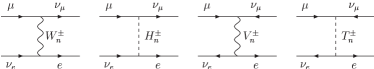
Figure 2: The tree-level Feynman diagrams for muon decays

The muon decay is dominated by exchanging $W^{\pm},V^{\pm}$ gauge boson and their KK excitations, see Fig.2. It also gets small contributions from exchanging physical charged Higgs from the doublet, the triplet and the anti-sextet. We can ignore these scalars contribution because they are suppressed by their Yukawa couplings.

The KK excitations of $W^{\pm}$ and $V^{\pm}$ give extra effective 4-fermion interactions as follows

$$\triangle H \sim \sum_{n=1}{g_{2}^{2}R^{2}}\left[{1\over(2n)^{2}}(\bar{\nu}_{\mu}\gamma^{\mu}P_{L}\mu)(\bar{e}\gamma_{\mu}P_{L}\nu_{e})\right.$$ (55)

$$+ \left.{{\cal U}^{*}_{ee}{\cal U}_{\mu\mu}\over(2n-1)^{2}}(\bar{\nu}_{\mu}\gamma^{\mu}P_{L}\mu^{\mathbf{c}})(\bar{e^{\mathbf{c}}}\gamma_{\mu}P_{L}\nu_{e})\right]$$

$$= g^{2}_{2}{\pi^{2}R^{2}\over 24}\left[(\bar{\nu}_{\mu}\gamma^{\mu}P_{L}\nu_{e})(\bar{e}\gamma_{\mu}P_{L}\mu)\right.$$

$$- \left.3\,{\cal U}^{*}_{ee}{\cal U}_{\mu\mu}(\bar{\nu}_{e}\gamma^{\mu}P_{L}\nu_{\mu})(\bar{e}\gamma_{\mu}P_{R}\mu)\right]$$

where ${\cal U}=U_{L}^{\dagger}U_{R}^{*}$ and $U_{L}$ is the unitary matrix that rotates the $SU(2)$ doublet leptons into their mass eigenstates, as discussed in section II.

The first term adds to the contribution from $W$ boson which is the zero mode and gives the dominant renormalization of the usual Fermi coupling $G_{F}^{\mu}$ BMar :

$$G_{F}^{\mu}\sim{\sqrt{2}g_{2}^{2}\over 8M_{W}^{2}}\left[1+{\pi^{2}M_{W}^{2}R^{2}\over 12}\right].$$ (56)

This correction is universal for all leptons and quarks. The contribution of $V$ gives non-zero $g^{S}_{RR}$ coefficient

$$g^{S}_{RR}={(\pi M_{W}R)^{2}\over 2}{\cal U}^{*}_{ee}{\cal U}_{\mu\mu}$$

in the notations of PDG . It has an upper bound $|g^{S}_{RR}|<{(\pi M_{W}R)^{2}\over 2}<0.018$. This in turn will modify the Michel parameters $\xi$ and $\rho$ to

$$\xi=1-{|g^{S}_{RR}|^{2}\over 4},\,\rho=\frac{3}{4}\left(1+{|g^{S}_{RR}|^{2}\over 4}\right).$$ (57)

But the deviations from the SM are $-8.1\times 10^{-5}<(\xi-1)<0$ and $0<(\rho-0.75)<6.1\times 10^{-5}$. They are beyond the reach of currently available experiments. Also the branch ratio of lepton number violation $\mu^{+}\rightarrow e^{+}\bar{\nu_{e}}\nu_{\mu}$ decay can be estimated to be $\sim|g^{S}_{RR}|^{2}<10^{-4}$. This is insufficient to account for the LSND neutrino anomaly LSND .

V.2 Muonium-antimuonium conversion and $\mu\rightarrow 3e$

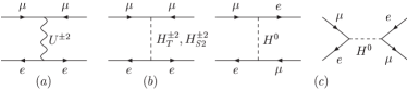
Figure 3: Tree-level diagrams for Muonium-antimuonium conversion.

The transition of muonium($M\equiv\mu^{+}e^{-}$) into antimuonium ($\overline{M}\equiv\mu^{-}e^{+}$) can be induced by the exchange of $U^{\pm 2}$ gauge boson or the scalar KK modes ${H_{T}}^{\pm 2},H_{S2}^{\pm 2}$ which belong to the $\bar{\mathbf{6}}$ ( see Fig.3(a,b)). It also can be induced by lepton number conserving but flavor changing neutral scalars or pseudoscalars as in Fig.3(c).

The $M-\overline{M}$ transition amplitude is written in terms of the mixing

$${\delta\over 2}\equiv\left\langle\overline{M}|H_{M\overline{M}}|M\right\rangle.$$ (58)

Using this, the transition possibility is calculated to be $P_{M\overline{M}}\sim\delta^{2}/2\Gamma_{\mu}^{2}$ normalized to muon decay rate $\Gamma_{\mu}=G_{F}^{2}m_{\mu}^{5}/192\pi^{3}$. The mixing $\delta$ is sensitive to the helicity structure of the interaction $H_{M\overline{M}}$ and the total spin of the muonium, for details see MAMC . Fig.3(a), gives a $(V\pm A)(V\mp A)$-type of effective Hamiltonian:

$$H^{U}_{M\overline{M}}={G^{U}_{M\overline{M}}\over\sqrt{2}}[\bar{\mu}\gamma^{\nu}(1-\gamma_{5})e][\bar{\mu}\gamma^{\nu}(1+\gamma_{5})e]+H.c.$$ (59)

with the effective Fermi constant given by

$${G^{U}_{M\overline{M}}\over\sqrt{2}}=\sum_{n=1}{(\sqrt{2}g_{2})^{2}\over 8M_{Un}^{2}}|{\cal U}^{*}_{ee}{\cal U}_{\mu\mu}|={g_{2}^{2}\pi^{2}R^{2}\over 32}|{\cal U}^{*}_{ee}{\cal U}_{\mu\mu}|.$$ (60)

Assuming that the external magnetic field is zero, we have $\delta^{U}_{3}=-8G^{U}_{M\overline{M}}/\sqrt{2}\pi a^{3}$ for the triplet muonium state and $\delta^{U}_{1}=+24G^{U}_{M\overline{M}}/\sqrt{2}\pi a^{3}$ for the singlet muonium where $a=(\alpha m_{e})^{-1}$ is the Bohr radius.

The relevant lepton number violating scalar interaction, see Fig. 3(b), can be parameterized as

$${\cal L}_{\not L}=\sum_{n=1}\left[f^{T}_{ij}\bar{l^{\mathbf{c}}}_{i}P_{L}l_{j}H^{+2}_{T,n}+f^{S}_{ij}\bar{l^{\mathbf{c}}}_{i}P_{R}l_{j}H^{+2}_{S2,n}\right]+H.c.$$ (61)

which leads to $(V\pm A)^{2}$-type effective Hamiltonian. With the help of Fierz transformations, we obtain the effective Hamiltonian

$$H^{\not L}_{M\overline{M}}=\sum_{n=1}f^{T}_{\mu\mu}f^{T}_{ee}{[\bar{\mu}\gamma^{\nu}(1-\gamma_{5})e]^{2}\over 8M^{2}_{Tn}}$$

$$+\sum_{n=1}f^{S}_{\mu\mu}f^{S}_{ee}{[\bar{\mu}\gamma^{\nu}(1+\gamma_{5})e]^{2}\over 8M^{2}_{Sn}}+H.c.$$ (62)

where $f^{T}=(U_{L}^{T}f_{6}U_{L})/\sqrt{2\pi RM^{*}}$ and $f^{S}=(U_{R}^{T}f_{6}U_{R})/\sqrt{2\pi RM^{*}}$. Since $(V+A)^{2}$ and $(V-A)^{2}$ give same contribution to the mixing matrix element, we can simply add them up and arrive at

$${G^{\not L}_{M\overline{M}}\over\sqrt{2}}\sim{\pi^{2}R^{2}\over 64}(f^{T}_{\mu\mu}f^{T}_{ee}+f^{S}_{\mu\mu}f^{S}_{ee}).$$ (63)

The lepton number violating interaction due to doubly charged scalars contributes an amount $\delta^{\not L}=16G^{\not L}_{M\overline{M}}/\sqrt{2}\pi a^{3}$ to the $M-\overline{M}$ mixing for both muonium singlet and triplet states. Despite the appearance note that the relative sign between contributions from $U$ gauge boson and $H_{S2},H_{T}$ scalars is not determined until the details of Yukawa couplings and mixing matrix ${\cal U}$ are known.

Next, we turn our attention to the transition due to flavor changing neutral scalars, see Fig.3(c). First, let us parameterize the interaction as

$${\cal L}_{\rm FC}=f^{\mu e}_{i}\sum_{i,n=0}\kappa_{n}\bar{\mu}eH^{0}_{in}+if^{\mu e}_{P_{i}}\sum_{i,n=0}\kappa_{n}\bar{\mu}\gamma_{5}eH^{0}_{P_{i}n}+H.c.$$ (64)

where $H^{0}_{in}$ stands for the n-th KK mode of physical neutral scalar-$i$ and $H_{P}$ is the physical pseudoscalar-$i$. In this model, we have two physical neutral scalar zero modes and one physical pseudoscalar zero mode. Generally speaking, one linear combination of the fifth component of gauge boson and the two scalar KK modes will be the Goldstone boson that is the KK gauge boson longitudinal component. So we are still left with three physical neutral KK scalars and three KK pseudoscalar for each KK level from $\phi_{3},\phi_{3}^{\prime}$ and $\phi_{6}$. The linear combination depends on the details of how the 5D gauge is fixed, such details can be ignored for we just need a qualitative analysis here.

The above lagrangian induces a effective Hamiltonian

$$H_{SP}={G^{S}_{M\overline{M}}\over\sqrt{2}}(\bar{\mu}e)^{2}-{G^{P}_{M\overline{M}}\over\sqrt{2}}(\bar{\mu}\gamma_{5}e)^{2}+H.c.$$ (65)

with

$${G^{S}_{M\overline{M}}\over\sqrt{2}} \sim \sum_{i}(f^{\mu e}_{++i})^{2}\left[{1\over M^{2}_{Hi}}+{(\pi R)^{2}\over 12}\right]$$

$$+ (f^{\mu e}_{+-})^{2}{(\pi R)^{2}\over 4}$$

$${G^{P}_{M\overline{M}}\over\sqrt{2}} \sim (f^{\mu e}_{++P})^{2}\left[{1\over M^{2}_{P}}+{(\pi R)^{2}\over 12}\right]$$

$$+ \sum_{i}(f^{\mu e}_{+-P_{i}})^{2}{(\pi R)^{2}\over 4}$$

where $M_{Hi}$ and $M_{P}$ are the zero mode masses for $(++)$-parity scalars and pseudoscalar.

The resulting mixings are

$$\delta^{SP}_{1}=(4G^{S}_{M\overline{M}}-8G^{P}_{M\overline{M}})/\sqrt{2}\pi a^{3}$$ (66)

for singlet state and

$$\delta^{SP}_{3}=-4G^{S}_{M\overline{M}}/\sqrt{2}\pi a^{3}$$ (67)

for the triplet state.

Clearly, more information on the new physics can be obtained if experiments can be done with separated muonium singlet and triplet states. To make things simple, we will just assume the muonium is prepared in a statistical mixture; namely $25\%$ is in singlet state and $75\%$ is in triplet state. Then we derive the transition probability to be:

$$P(\overline{M})\sim 64^{2}\left({6\pi^{2}\alpha^{3}\over G_{F}m_{\mu}^{2}}\right)^{2}\left({m_{e}\over m_{\mu}}\right)^{6}\left({\overline{G}_{M\overline{M}}\over G_{F}}\right)^{2}$$

$$=1.75\times 10^{-6}\left({\overline{G}_{M\overline{M}}\over G_{F}}\right)^{2}$$ (68)

where the effective 4 fermion coupling constant is

$$\overline{G}^{2}_{M\overline{M}}=\frac{1}{4}\left[-2G^{U}_{M\overline{M}}+4G_{M\overline{M}}^{\not L}+G_{M\overline{M}}^{S}-2G_{M\overline{M}}^{P}\right]^{2}$$

$$+\frac{3}{4}\left[6G_{M\overline{M}}^{U}+4G_{M\overline{M}}^{\not L}-G_{M\overline{M}}^{S}\right]^{2}\,.$$ (69)

The present experimental bound $P_{M\overline{M}}<8.3\times 10^{-11}$ Willmann:1998gd requires that $\overline{G}_{M\overline{M}}<6.9\times 10^{-3}G_{F}$. Obviously, the actual number of $\overline{G}_{M\overline{M}}$ strongly depend on the pattern of Yukawa couplings. For brevity, we will just discuss constraints from two simplified Yukawa patterns: (1) The diagonal $f_{6}$ case as discussed in SU3:triumf and (2) the democratic patterns which will be discussed below.

First, we will consider the diagonal Yukawa pattern with $f^{6}_{ij}\propto\delta_{ij}m_{i}/M_{W}$ and $f_{3}\sim f^{\prime}_{3}\ll f^{6}$. Since the charged lepton masses are mainly controlled by the Yukawa couplings of the $\bar{\mathbf{6}}$ all the Yukawa couplings are expected to be suppressed by $m_{l}/M_{W}$ and the transition is mainly due to $U$ gauge boson. In this case, the effective $\overline{G}_{M\overline{M}}$ can be simplified to:

$${\overline{G}_{M\overline{M}}\over G_{F}}\sim\sqrt{28}{G^{U}_{M\overline{M}}\over G_{F}}=-20.93\times 10^{-3}\left({2\mbox{TeV}\over 1/R}\right)^{2}\times|{\cal U}^{*}_{ee}{\cal U}_{\mu\mu}|\,.$$ (70)

Here the lepton mass eigenstates and gauge eigenstates almost coincide, the mixing is nearly diagonal ${\cal U}^{*}_{ee}\sim{\cal U}_{\mu\mu}\sim 1$. To stay under the experimental bound one requires $1/R>3.48$ TeV. From the discussion of unification we see that such high compactification scale is not impossible when the factor $\pi RM_{G}$ is less than $10$. Note that the unification scale $M_{G}$ needs not be the fundamental scale $M^{*}$. Therefore, even in this case one can still have large volume dilution factor required by the strong coupling assumption.

But this argument does not apply to the flavor changing channel mediated by neutral scalars whose Yukawa couplings are not proportional to lepton masses. For example, in this model $\phi^{\prime}_{3}$ has nothing to do with charged lepton masses and the flavor changing Yukawa coupling is roughly of the amount $f^{\prime}_{3}|f^{3}/f^{6}|$ which is not a severe suppression factor. Also, there are two physical neutral scalars and one physical pseudoscalar which have zero modes with masses around a few hundred GeV. This is to be compared to the masses of $U^{\pm 2}$ which is around few TeV. If these scalars have approximately two orders of magnitude enhanced couplings they can be as important as the $U$’s. Moreover, the resulting constraints can be relaxed or tighten depends on the relative sign between the contribution of vector bileptons and the flavor changing neutral scalars. Hence, no firm conclusion with regard to these scalars. We shall proceed by assuming they do not make important contributions.

Next, we study the following so called democratic Yukawa structure whose leading order is:

$$f_{6}\sim 0.1\left(\begin{array}[]{ccc}1&1&1\\ 1&1&1\\ 1&1&1\end{array}\right),\hskip 8.53581ptf_{3}\sim 0.01\left(\begin{array}[]{ccc}0&1&1\\ -1&0&1\\ -1&-1&0\end{array}\right)\,.$$ (71)

Our numerical search indicates that it is easy to get realistic solutions which yield observed charged lepton mass hierarchy and give $|{\cal U}^{*}_{ee}{\cal U}_{\mu\mu}|<0.1$. In that case, basically the $M-\bar{M}$ conversion posts no constraint on $1/R$. One might wonder if this Yukawa pattern will change neutrino mass pattern. Correspondingly, we found a simple pattern of $y^{\prime}_{3}$ with $f^{{}^{\prime}3}_{12}:f^{{}^{\prime}3}_{13}:f^{{}^{\prime}3}_{23}\sim 1:m_{\mu}/m_{\tau}:m_{e}/m_{\tau}$ which can gives desired bi-large mixing neutrino mass matrix of inverted hierarchy type.

Nevertheless, we expect the constraint can be loosen once the contributions from the Higgs sectors are included. The Yukawa coupling pattern can be arranged such that either the coupling of $U$ is tiny or the scalars come in and play a significant role to balance the contribution form $U^{\pm 2}$ gauge boson. To find such a pattern is a nontrivial task which we shall leave it to future investigations and assume $1/R\sim 1.5-3.5$ TeV is viable for the rest part of the paper.

We note in passing that the supersymmetrical version of this model will push the unification scale $1/R$ to $\sim 6$ TeVorbifold_SU3 . Which will significantly suppress this process but make it less interesting for collider search.

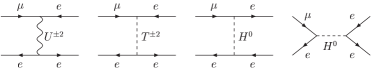
Figure 4: Tree-level diagrams for $\mu\rightarrow 3e$.

The diagrams of Fig. 4 will lead to $\mu\rightarrow 3e$ transition. The amplitude is

$$i{\cal M} = (ig)^{2}\sum_{n=1}{-2i\over u-M_{Un}^{2}}\left[\bar{e}\gamma^{\mu}{P_{L}-P_{R}\over 2}{\cal U}_{ee}e^{\mathbf{c}}\right]\left[\bar{e^{\mathbf{c}}}\gamma_{\mu}{P_{L}{\cal U}^{*}_{\mu e}-P_{R}{\cal U}^{*}_{e\mu}\over 2}\mu\right]$$ (72)

$$+ (i\sqrt{2}(f_{T})_{e\mu})(i\sqrt{2}(f_{T}^{\dagger})_{ee})\sum_{n=1}{2i\over u-M_{Tn}^{2}}\left[\bar{e^{\mathbf{c}}}P_{L}\mu\right]\left[\bar{e}P_{R}e^{\mathbf{c}}\right]+\ldots$$

where the dots represent the possible flavor changing neutral current ( FCNC ) scalar couplings. After Fierz rearrangement, we have the effective Lagrangian for the decay:

$${\cal L} = \sum_{n=1}{g_{2}^{2}{\cal U}_{ee}\over M_{Un}^{2}}\left\{(\bar{e}\gamma^{\mu}P_{L}\mu)(\bar{e}\gamma_{\mu}P_{R}e){\cal U}^{*}_{\mu e}+(\bar{e}\gamma^{\mu}P_{R}\mu)(\bar{e}\gamma_{\mu}P_{L}e){\cal U}^{*}_{e\mu}\right\}$$ (73)

$$+\sum_{n=1}{2(f_{T})_{e\mu}(f_{T}^{*})_{ee}\over M_{Tn}^{2}}[(\bar{\mu}\gamma^{\mu}P_{L}e)(\bar{e}\gamma_{\mu}P_{L}e)]+H.c.+\ldots$$

$$= {(g_{2}\pi R)^{2}\over 8}\left\{(\bar{e}\gamma^{\mu}P_{L}\mu)(\bar{e}\gamma_{\mu}P_{R}e){\cal U}_{ee}{\cal U}^{*}_{\mu e}+(\bar{e}\gamma^{\mu}P_{R}\mu)(\bar{e}\gamma_{\mu}P_{L}e){\cal U}_{ee}{\cal U}^{*}_{e\mu}\right.$$

$$\left.+2(f_{T})_{e\mu}(f_{T}^{*})_{ee}(\bar{\mu}\gamma^{\mu}P_{L}e)(\bar{e}\gamma_{\mu}P_{L}e)\right\}+H.c.+\ldots$$

The branching ratio is given by

$$Br(\mu\rightarrow 3e)={(g_{2}\pi R)^{4}\over 512G_{F}^{2}}\left\{(|{\cal U}_{\mu e}|^{2}+|{\cal U}_{e\mu}|^{2})|{\cal U}_{ee}|^{2}+8|(f_{T})_{e\mu}(f_{T}^{*})_{ee}|^{2}+\ldots\right\}\,.$$

Note that the scalar contribution here is positive. For simplicity, we will only keep the contribution of $U^{\pm 2}$ for estimation:

$$Br(\mu\rightarrow 3e)\sim 1.56\times 10^{-5}\left(2\mbox{TeV}\over 1/R\right)^{4}\left(|{\cal U}_{\mu e}|^{2}+|{\cal U}_{e\mu}|^{2}\right)|{\cal U}_{ee}|^{2}\,.$$ (74)

The experimental limit $Br(\mu\rightarrow 3e)<1.0\times 10^{-12}$ leads to the requirement that the mixing combination $(|{\cal U}_{\mu e}|^{2}+|{\cal U}_{e\mu}|^{2})|{\cal U}_{ee}|^{2}$ to be very small. In the diagonal $f_{6}$ case, ${\cal U}_{ee}\sim 1$ but the mixing ${\cal U}_{\mu e}$ and ${\cal U}_{e\mu}$ are suppressed by a factor of $\sim(f_{3}/f_{6})$ of small $\phi_{3}$ Yukawa coupling. Since theory consistence set a upper bound of $1/R\sim 5$ TeV, the FCNC couplings must satisfy $|{\cal U}_{\mu e}|,|{\cal U}_{\mu e}|<1.1\times 10^{-3}$. On the other hand, in the democrat Yukawa case the mixing can be made very small so as to evade this constraint. This demonstrates that in future model building these constraints has to be taken into account and Yukawa couplings are not totally arbitrary.

Similarly, we have the following rare decay branching ratios for $\tau$:

$$Br(\tau\rightarrow 3\mu) = 1.56\times 10^{-5}\left(2\mbox{TeV}\over 1/R\right)^{4}\left(|{\cal U}_{\tau\mu}|^{2}+|{\cal U}_{\mu\tau}|^{2}\right)|{\cal U}_{\mu\mu}|^{2}\,,$$ (75)

$$Br(\tau\rightarrow 3e) = 1.56\times 10^{-5}\left(2\mbox{TeV}\over 1/R\right)^{4}\left(|{\cal U}_{\tau e}|^{2}+|{\cal U}_{e\tau}|^{2}\right)|{\cal U}_{ee}|^{2}\,,$$ (76)

$$Br(\tau\rightarrow\bar{\mu}ee) = 1.56\times 10^{-5}\left(2\mbox{TeV}\over 1/R\right)^{4}\left(|{\cal U}_{\tau\mu}|^{2}+|{\cal U}_{\mu\tau}|^{2}\right)|{\cal U}_{ee}|^{2}\,,$$ (77)

$$Br(\tau\rightarrow\mu\mu\bar{e}) = 1.56\times 10^{-5}\left(2\mbox{TeV}\over 1/R\right)^{4}\left(|{\cal U}_{\tau e}|^{2}+|{\cal U}_{e\tau}|^{2}\right)|{\cal U}_{\mu\mu}|^{2}\,,$$ (78)

$$Br(\tau\rightarrow\mu e\bar{e}) = 1.95\times 10^{-6}\left(2\mbox{TeV}\over 1/R\right)^{4}\left(|{\cal U}_{\tau e}|^{2}+|{\cal U}_{e\tau}|^{2}\right)\left(|{\cal U}_{e\mu}|^{2}+|{\cal U}_{\mu e}|^{2}\right)\,,$$ (79)

$$Br(\tau\rightarrow e\mu\bar{\mu}) = 1.95\times 10^{-6}\left(2\mbox{TeV}\over 1/R\right)^{4}\left(|{\cal U}_{\tau\mu}|^{2}+|{\cal U}_{\mu\tau}|^{2}\right)\left(|{\cal U}_{e\mu}|^{2}+|{\cal U}_{\mu e}|^{2}\right)\,.$$ (80)

But the current limit $\sim 3\times 10^{-6}$ does not impose strong constraint on the mixing. Because the scalar sector gives positive contribution to these rare decays, from the unitarity of ${\cal U}$ the model predicts an interesting lower bond for a given $1/R$

$$Br(\tau\rightarrow 3e)>3.12\times 10^{-5}\left(2\mbox{TeV}\over 1/R\right)^{4}|{\cal U}_{ee}|^{2}\left(1-|{\cal U}_{ee}|^{2}\right)\,.$$ (81)

If one wants to keep compactification scale $1/R$ low, say $\sim 1.5$ TeV, it is required that $|{\cal U}_{ee}|$ to be either close to zero or one. Furthermore, if we take the upper bound of $1/R<5$ TeV derived from unification seriously we obtain

$$Br(\tau\rightarrow 3e)>8.0\times 10^{-7}|{\cal U}_{ee}|^{2}\left(1-|{\cal U}_{ee}|^{2}\right)\,.$$ (82)

On the other hand, if we assume that the bilepton exchange is the dominate FCNC source, another interesting upper bond can be derived:

$$Br(\tau\rightarrow 3e)<7.8\times 10^{-6}\left(2\mbox{TeV}\over 1/R\right)^{4}.$$ (83)

An observation of this decay will shed light on the Yukawa structure.

VI Collider Signatures

In collider experiments the bilepton signals can be directly probed. For simplicity, in the following discussion we will not consider the contribution from scalar bileptons due to the Yukawa suppression.

VI.1 $l^{+}l^{-}$ scattering

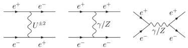
Figure 5: Feynman diagrams for $e^{+}e^{-}$ scattering.

First we consider the high energy Bhabha scattering, $e^{-}(p_{1})e^{+}(p_{2})\rightarrow e^{-}(p_{3})e^{+}(p_{4})$, see Fig.5. The amplitude from $u$-channel $U^{\pm 2}$ KK tower exchange is given by:

$$i{\cal M}_{U}=\sum_{n=1}{-i(ig_{2})^{2}(2!)^{2}|{\cal U}_{ee}|^{2}\over u-M_{n}^{2}+iM_{n}\Gamma_{n}}\left(\bar{u}(p_{3})\gamma_{\mu}{P_{L}-P_{R}\over 2}C\bar{v}^{T}(p_{2})\right)\left(-v^{T}(p_{4})C^{-1}\gamma^{\mu}{P_{L}-P_{R}\over 2}u(p_{1})\right)\,.$$ (84)

By Fierz transformation, it can be rearranged to

$${\cal M}_{U}=\left.\sum_{n=1}{-g_{2}^{2}|{\cal U}_{ee}|^{2}\over u-M_{n}^{2}+iM_{n}\Gamma_{n}}\right[\bar{u}(p_{3})\gamma_{\mu}P_{L}u(p_{1})\bar{v}(p_{2})\gamma^{\mu}P_{R}v(p_{4})+\bar{u}(p_{3})\gamma_{\mu}P_{R}u(p_{1})\bar{v}(p_{2})\gamma^{\mu}P_{L}v(p_{4})$$

$$\left.-\bar{u}(p_{3})\gamma_{\mu}P_{L}v(p_{4})\bar{v}(p_{2})\gamma^{\mu}P_{R}u(p_{1})-\bar{u}(p_{3})\gamma_{\mu}P_{R}v(p_{4})\bar{v}(p_{2})\gamma^{\mu}P_{L}u(p_{1})\stackrel{{\scriptstyle\mbox{$\,$ }}}{{\mbox{}}}\right]\,.$$ (85)

The minus signs in front of the last two terms are due to Fermi statistics. We use the Mandelstam variables in the following and combine all the contribution from $U,\gamma,Z$ and their KK excitations. The total transition amplitude can be written as

$${\cal M}(e^{+}e^{-}\rightarrow e^{+}e^{-})=$$ (86)

$$g_{2}^{2}G^{B}_{\lambda,\lambda^{\prime}}\bar{u}(p_{3})\gamma^{\mu}P_{\lambda}v(p_{4})\bar{v}(p_{2})\gamma_{\mu}P_{\lambda^{\prime}}u(p_{1})$$

$$- g_{2}^{2}F^{B}_{\lambda,\lambda^{\prime}}\bar{v}(p_{2})\gamma^{\mu}P_{\lambda}v(p_{4})\bar{u}(p_{3})\gamma_{\mu}P_{\lambda^{\prime}}u(p_{1})$$

where $\lambda,\lambda^{\prime}=L,R$. The coefficients are the sums of all KK excitation as well as SM gauge bosons and they read

$$G^{B}_{\lambda,\lambda^{\prime}} = s_{W}^{2}\sum_{n=0}{\kappa_{n}^{2}\over s-M_{\gamma n}^{2}+iM_{\gamma n}\Gamma_{\gamma n}}$$ (87)

$$+ {g_{\lambda}g_{\lambda^{\prime}}\over c_{W}^{2}}\sum_{n=0}{\kappa_{n}^{2}\over s-M_{Zn}^{2}+iM_{Zn}\Gamma_{Zn}}$$

$$- (1-\delta_{\lambda,\lambda^{\prime}})\sum_{n=1}{g^{B}_{\lambda,\lambda^{\prime}}\over u-M_{Un}^{2}+iM_{Un}\Gamma_{Un}}$$

where $g^{B}_{\lambda,\lambda^{\prime}}=|{\cal U}_{ee}|^{2}$, $g_{L}=s_{W}^{2}-1/2$ and $g_{R}=s_{W}^{2}$. Similarly,

$$F^{B}_{\lambda,\lambda^{\prime}} = s_{W}^{2}\sum_{n=0}{\kappa_{n}^{2}\over t-M_{\gamma n}^{2}+iM_{\gamma n}\Gamma_{\gamma n}}$$ (88)

$$+ {g_{\lambda}g_{\lambda^{\prime}}\over c_{W}^{2}}\sum_{n=0}{\kappa_{n}^{2}\over t-M_{Zn}^{2}+iM_{Zn}\Gamma_{Zn}}$$

$$- (1-\delta_{\lambda,\lambda^{\prime}})\sum_{n=1}{f^{B}_{\lambda,\lambda^{\prime}}\over u-M_{Un}^{2}+iM_{Un}\Gamma_{Un}}$$

with $f^{B}_{\lambda,\lambda^{\prime}}=|{\cal U}_{ee}|^{2}$.

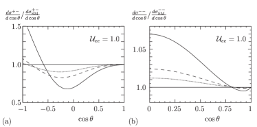
Figure 6: The ratio of differential cross section to that of SM at $\sqrt{s}=500$ GeVfor(a) the Bhabha and (b)Møller scattering. The mixing ${\cal U}_{ee}$ is set to 1.Solid:$1/R=1.5$ TeV, Dash:$1/R=2.5$ TeV; Dotted: $1/R=3.5$ TeV.

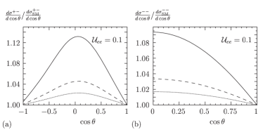
Figure 7: Same as previous fig.6 but ${\cal U}_{ee}=0.1$.

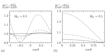
Figure 8: Same as figure 6 with $1/R=2.5$TeV and ${\cal U}_{ee}=0.5$. The center of mass energy of collider $\sqrt{s}=500$ GeV(Solid), $800$ GeV(Dash) and $1.5$TeV(Dotted).

The differential cross section can be calculated straightforwardly

$${d\sigma^{+-}\over d\cos\theta} = {\pi\alpha^{2}s\over 2s_{W}^{4}}\left[|F^{B}_{RL}|^{2}+|F^{B}_{LR}|^{2}+(|G^{B}_{RL}|^{2}+|G^{B}_{LR}|^{2}){t^{2}\over s^{2}}\right.$$ (89)

$$+ \left.{u^{2}\over s^{2}}(|G^{B}_{LL}+F^{B}_{LL}|^{2}+|G^{B}_{RR}+F^{B}_{RR}|^{2})\right]$$

with $F^{B}_{LR}=F^{B}_{RL}$ and $G^{B}_{LR}=G^{B}_{RL}$. The deviation from the SM prediction are displayed in the panel-(a) of Figs.6, 7, 8 for some typical parameter sets.

Of course, in $e^{+}e^{-}$ experiments, a signal of flavor changing scattering $e^{+}e^{-}\rightarrow l^{+}_{i}l^{-}_{j},i\neq j$ is clearly beyond SM. In this model, it could be mediated by flavor changing coupling of $U^{\pm 2}$ gauge bosons. Also, there is possible small contribution from $t-$channel FCNC Higgs and scalar bilepton diagrams. From our discussion above, the cross section is already at hand. We just substitute it with the following nonzero variables

$$F^{B}_{\lambda,\lambda^{\prime}}=-\sum_{n=1}{(1-\delta_{\lambda,\lambda^{\prime}})f^{B}_{\lambda,\lambda^{\prime}}\over u-M_{Un}^{2}+iM_{Un}\Gamma_{Un}}$$

$$G^{B}_{\lambda,\lambda^{\prime}}=-\sum_{n=1}{(1-\delta_{\lambda,\lambda^{\prime}})g^{B}_{\lambda,\lambda^{\prime}}\over u-M_{Un}^{2}+iM_{Un}\Gamma_{Un}}$$

in different cases:

$$i,j\neq e : f^{B}_{RL}={{\cal U}^{*}_{ei}{\cal U}_{je}\over 4},\,f^{B}_{LR}={{\cal U}^{*}_{ie}{\cal U}_{ej}\over 4},$$ (90)

$$g^{B}_{RL}={{\cal U}^{*}_{ei}{\cal U}_{ej}\over 4},\,g^{B}_{LR}={{\cal U}^{*}_{ie}{\cal U}_{je}\over 4}\,,$$

$$j=e : f^{B}_{RL}=g^{B}_{RL}={{\cal U}_{ee}{\cal U}^{*}_{ei}\over 2},$$ (91)

$$f^{B}_{LR}=g^{B}_{LR}={{\cal U}_{ee}{\cal U}^{*}_{ie}\over 2}\,,$$

$$i=e : f^{B}_{RL}=g^{B}_{LR}={{\cal U}^{*}_{ee}{\cal U}_{je}\over 2},$$ (92)

$$f^{B}_{LR}=g^{B}_{RL}={{\cal U}^{*}_{ee}{\cal U}_{ej}\over 2}\,.$$

Then the different flavor violating scattering channels can be used to fix off-diagonal entities of mixing matrix $\cal U$.

VI.2 $l^{-}l^{-}$ scattering

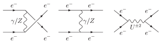
Figure 9: Diagrams for $e^{-}e^{-}$ scattering.

Similarly, the amplitude for Møller scattering, see fig.9, is expressed as

$${\cal M}(e^{-}e^{-}\rightarrow e^{-}e^{-})=$$ (93)

$$g_{2}^{2}G^{M}_{\lambda,\lambda^{\prime}}\bar{u}(p_{4})\gamma^{\mu}P_{\lambda}u(p_{2})\bar{u}(p_{3})\gamma_{\mu}P_{\lambda^{\prime}}u(p_{1})$$

$$- g_{2}^{2}F^{M}_{\lambda,\lambda^{\prime}}\bar{u}(p_{3})\gamma^{\mu}P_{\lambda}u(p_{2})\bar{u}(p_{4})\gamma_{\mu}P_{\lambda^{\prime}}u(p_{1})$$

where

$$F^{M}_{\lambda,\lambda^{\prime}} = s_{W}^{2}\sum_{n=0}{\kappa_{n}^{2}\over u-M_{\gamma n}^{2}+iM_{\gamma n}\Gamma_{\gamma n}}$$ (94)

$$+ {g_{\lambda}g_{\lambda^{\prime}}\over c_{W}^{2}}\sum_{n=0}{\kappa_{n}^{2}\over u-M_{Zn}^{2}+iM_{Zn}\Gamma_{Zn}}$$

$$- (1-\delta_{\lambda,\lambda^{\prime}})\sum_{n=1}{f^{M}_{\lambda,\lambda^{\prime}}\over s-M_{Un}^{2}+iM_{Un}\Gamma_{Un}}$$

and

$$G^{M}_{\lambda,\lambda^{\prime}} = s_{W}^{2}\sum_{n=0}{\kappa_{n}^{2}\over t-M_{\gamma n}^{2}+iM_{\gamma n}\Gamma_{\gamma n}}$$ (95)

$$+ {g_{\lambda}g_{\lambda^{\prime}}\over c_{W}^{2}}\sum_{n=0}{\kappa_{n}^{2}\over t-M_{Zn}^{2}+iM_{Zn}\Gamma_{Zn}}$$

$$- (1-\delta_{\lambda,\lambda^{\prime}})\sum_{n=1}{g^{M}_{\lambda,\lambda^{\prime}}\over s-M_{Un}^{2}+iM_{Un}\Gamma_{Un}}$$

with $f^{M}_{\lambda,\lambda^{\prime}}=g^{M}_{\lambda,\lambda^{\prime}}=|{\cal U}_{ee}|^{2}$. The differential cross section is

$${d\sigma^{--}\over d\cos\theta}={\pi\alpha^{2}s\over 4s_{W}^{4}}\left[|G^{M}_{LL}+F^{M}_{LL}|^{2}+|G^{M}_{RR}+F^{M}_{RR}|^{2}\right.$$

$$\left.+{u^{2}\over s^{2}}(|G^{M}_{LR}|^{2}+|G^{M}_{RL}|^{2})+{t^{2}\over s^{2}}(|F^{M}_{LR}|^{2}+|F^{M}_{RL}|^{2})\right]\,.$$ (96)

The angular distribution is also different from the SM prediction, see panel-(b) of Figs.6, 7, 8 illustrated with some typical parameter sets. Besides comparing the angular distribution with the SM prediction, the flavor changing production $e^{-}e^{-}\rightarrow l^{\prime-}l^{-},\,(l^{\prime},l\neq e)$ in a linear collider will be a very clean signal which can only be due to bilepton exchange. For example, the $e^{-}e^{-}\rightarrow\mu^{-}\mu^{-}$ cross section is given by

$${d\sigma\over d\cos\theta}={g_{2}^{4}\over 32\pi s}(1+\cos\theta^{2})\left|\sum_{n=1}{s{\cal U}^{*}_{ee}{\cal U}_{\mu\mu}\over s-M_{Un}^{2}+iM_{Un}\Gamma_{Un}}\right|^{2}$$ (97)

where $\cos\theta$ goes from $0$ to $1$ due to the final states are identical particles. If we take ${\cal U}^{*}_{ee}{\cal U}_{\mu\mu}=1$, the total cross section is $(2.5,0.3,0.1)fb$ at $\sqrt{s}=100$ GeV for $1/R=(1.5,2.5,3.5)$TeV respectively, but increase to $(74.1,8.4,2.1)$fb at $\sqrt{s}=500$ GeV and $(666.7,42.2,9.5)fb$ at $\sqrt{s}=1$ TeV. The same expression, with the appropriate substitutions for the mixing factors, applies also to $e^{-}e^{-}\rightarrow\tau^{-}\tau^{-}$ and $\mu^{-}\mu^{-}\rightarrow\tau^{-}\tau^{-}$ cross sections. These will be unmistakable existence signals of bilepton $U^{\pm 2}$. For other flavor changing scattering, $e^{-}e^{-}\rightarrow e^{-}\mu^{-},\tau^{-}\mu^{-},\cdots$ etc, it is easy to get the corresponding expression from Eq. (97).

VI.3 Gauge bosons pair production signature in colliders

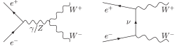
Figure 10: Diagrams for $W$ pair production in $e^{+}e^{-}$ collider.

The SM $W$-pair production is an important test of the SM. The tree level diagrams are shown in Fig.10 where we do not display the Higgs exchange graph. Here we discuss how will it be affected in the $SU(3)_{W}$ model. The first correction is due to exchanging KK photons and KK $Z$ bosons. But since the two final state $W^{\pm}$ are zero modes the KK number conservation at the triple gauge vertex forces the virtual neutral gauge boson to be a zero mode too. Since the fermions are 4D brane fields in this model, nothing will be added to the $t-$channel neutrino diagram. Thus, we conclude there is no tree-level correction to the SM $W$-pair production process.

Next, can the $W_{1}^{\pm}W^{\mp}$ be produced in a linear collider? This can proceed through the $s$ channel photon and $Z$ exchange $e^{+}e^{-}\rightarrow\gamma_{1}/Z_{1}\rightarrow W_{1}^{\pm}W^{\mp}$ and the $t$-channel neutrino exchanging diagrams. Both are allowed by KK number conservation. But the $W_{1}$ mass $\sim 2/R$ requires a linear collider with $\sqrt{s}>3$ TeV. If the collider is available, we shall also observe the pair production of the first KK modes of $U^{\pm 2}$ or $V^{\pm}$ gauge bosons. For example, $e^{+}e^{-}\rightarrow U^{+2}_{1}U^{-2}_{1}$ can be mediated by the zero modes and the first KK excitation of photon and $Z$ with distinctive signatures of $U^{\pm 2}$ bileptonic decays.

The pair production of bileptons can also be searched in the hadron collider through virtual photon or $Z$ coming from $\bar{q}q\rightarrow\gamma^{*}/Z^{*}\rightarrow U^{+2}U^{-2}$ or virtual $W$ from $\bar{q}q^{\prime}\rightarrow W^{*}\rightarrow UV$. For completeness, we also give triple gauge couplings in the appendix. Due to the high masses involved, a detail phenomenological analysis involving hadron machines is premature now.

VII $\nu e$ scattering

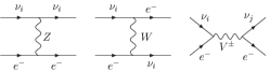
Figure 11: The Feynman diagrams for $\nu e$ scattering.

The low energy neutrino electron scattering is another place to look for new physics signals. The $\nu^{i}e\rightarrow\nu^{j}e$ process receives corrections form KK modes of $Z,W^{\pm}$ and $V^{\pm}$ gauge bosons, see Fig.11. The scattering amplitude reads

$$i{\cal M} = \sum_{n=0}\left({ig_{2}\kappa_{n}\over c_{W}}\right)^{2}{-i\over(p_{1}-p_{3})^{2}-M_{Zn}^{2}}(\bar{\nu}_{i}\gamma^{\mu}g_{L}^{\nu}P_{L}\nu_{i})(\bar{e}\gamma_{\mu}[g_{L}P_{L}+g_{R}P_{R}]e)$$

$$+ \sum_{n=0}\left({ig_{2}\kappa_{n}\over\sqrt{2}}\right)^{2}{-i\over(p_{1}-p_{4})^{2}-M_{Wn}^{2}}(\bar{\nu}_{i}\gamma^{\mu}P_{L}\nu_{i})(\bar{e}\gamma_{\mu}P_{L}e)+\sum_{n=1}\left({ig_{2}\kappa_{n}\over\sqrt{2}}\right)^{2}{-i{\cal U}_{ie}{\cal U}^{\dagger}_{je}\over(p_{1}+p_{3})^{2}-M_{Vn}^{2}}(\bar{\nu}_{j}\gamma^{\mu}P_{L}e^{\mathbf{c}})(\bar{e^{\mathbf{c}}}\gamma_{\mu}P_{L}\nu_{i})\,.$$

The momenta transfers can be ignored compared to the gauge boson masses we can rewrite it as

$${\cal M} \simeq -{g_{2}^{2}\over 2c_{W}^{2}}\left(\frac{1}{M_{Z}^{2}}+{\pi^{2}R^{2}\over 12}\right)(\bar{\nu}_{i}\gamma^{\mu}P_{L}\nu_{i})(\bar{e}\gamma_{\mu}[g_{L}P_{L}+g_{R}P_{R}]e)$$ (98)

$$- {g_{2}^{2}\over 2}\left(\frac{1}{M_{W}^{2}}+{\pi^{2}R^{2}\over 12}\right)(\bar{\nu}_{i}\gamma^{\mu}P_{L}\nu_{i})(\bar{e}\gamma_{\mu}P_{L}e)+{g_{2}^{2}\over 2}{{\cal U}_{ie}{\cal U}^{\dagger}_{je}\pi^{2}R^{2}\over 4}(\bar{\nu}_{j}\gamma^{\mu}P_{L}\nu_{i})(\bar{e}\gamma_{\mu}P_{R}e)\,.$$

We parameterize it in the standard effective Hamiltonian form with the effective Fermi constant $G_{F}^{\mu}$ given by Eq. (56):

$$H_{eff}={G^{\mu}_{F}\over\sqrt{2}}(\bar{\nu}_{i}\gamma^{\mu}(1-\gamma_{5})\nu_{j})(\bar{e}\gamma_{\mu}(g^{ij}_{V}-g^{ij}_{A}\gamma_{5})e)$$ (99)

with

$$g_{V}^{ee}\sim(2s_{W}^{2}-\frac{1}{2})\left(1+\epsilon t^{2}_{W}\right)+1-3\epsilon|{\cal U}_{ee}|^{2}\,,$$ (100)

$$g_{A}^{ee}\sim-\frac{1}{2}\left(1+\epsilon t^{2}_{W}\right)+1+3\epsilon|{\cal U}_{ee}|^{2}\,,$$ (101)

$$g_{V}^{\mu\mu}\sim(2s_{W}^{2}-\frac{1}{2})\left(1+\epsilon t^{2}_{W}\right)-3\epsilon|{\cal U}_{\mu e}|^{2}\,,$$ (102)

$$g_{A}^{\mu\mu}\sim-\frac{1}{2}\left(1+\epsilon t^{2}_{W}\right)+3\epsilon|{\cal U}_{\mu e}|^{2}\,,$$ (103)

$$g_{V}^{\tau\tau}\sim(2s_{W}^{2}-\frac{1}{2})\left(1+\epsilon t^{2}_{W}\right)-3\epsilon|{\cal U}_{\tau e}|^{2}\,,$$ (104)

$$g_{A}^{\tau\tau}\sim-\frac{1}{2}\left(1+\epsilon t^{2}_{W}\right)+3\epsilon|{\cal U}_{\tau e}|^{2}$$ (105)

where $t_{W}^{2}=\sin^{2}\theta_{W}/\cos^{2}\theta_{W}$ and $\epsilon\equiv(\pi RM_{W})^{2}/12$. In this model, only $V^{\pm}$ gauge bosons pay tribute to the neutrino flavor changing scattering and give

$$-g_{V}^{ji}=g_{A}^{ji}\sim 3\epsilon{\cal U}_{ie}{\cal U}^{\dagger}_{je}\,,\,i\neq j.$$ (106)

If seen, it is clearly physics beyond SM.

We are interested in the situation that the incoming neutrino scatters off the electron at rest, $\nu^{i}(E_{\nu})+e\rightarrow\nu^{j}+e(E_{e})$, as been measured in the current neutrino experiments. Define the electron recoil energy as $T=E_{e}-m_{e}$ then the effective Hamiltonian leads to the following cross section 'tHooft:ht in the regime $q^{2}\ll M_{W}^{2}$

$${d\sigma\over dT}={2G_{\mu}^{2}m_{e}\over\pi}\sum_{j}\left\{(g_{L}^{ij})^{2}+(g_{R}^{ij})^{2}\left(1-\frac{T}{E_{\nu}}\right)^{2}\right.$$

$$\left.-g_{L}^{ij}g_{R}^{ij}{m_{e}T\over E_{\nu}^{2}}\right\}$$ (107)

where $g_{L}^{ij}=(g_{V}^{ij}+g_{A}^{ij})/2$ and $g_{R}^{ij}=(g_{V}^{ij}-g_{A}^{ij})/2$. The sum over final neutrino species is taken as they are not detected in such experiments. For incoming anti-neutrino, as in the reactor neutrino experiments, the cross section for $\bar{\nu}^{i}e$ scattering is simply

$${d\sigma\over dT}={2G_{\mu}^{2}m_{e}\over\pi}\sum_{j}\left\{(g_{R}^{ij})^{2}+(g_{L}^{ij})^{2}\left(1-\frac{T}{E_{\nu}}\right)^{2}\right.$$

$$\left.-g_{L}^{ij}g_{R}^{ij}{m_{e}T\over E_{\nu}^{2}}\right\}.$$ (108)

Labeling $\phi$ as the angle which recoiled electron is deflected from the incident neutrino, it relates to $T$ as

$$\cos\phi={E_{\nu}+m_{e}\over E_{\nu}}\sqrt{{T\over T+2m_{e}}}.$$ (109)

The electron recoil energy is in the range of $0\leq T\leq E_{\nu}^{2}/(E_{\nu}+m_{e}/2)$. We denote $\xi(T)$ as the ratio of the modified differential cross section to the SM as follows

$${d\sigma\over dT}={d\sigma_{SM}\over dT}(1+\xi(T)).$$ (110)

For $|{\cal U}_{ee}|=1$, the plot of $\xi(T)$ vs $T$ for two ${}^{7}Be$ neutrino lines is given in fig.12. This model gives compatible but opposite corrections to the SM radiative correction Bahcall:1995mm on the electron recoil energy spectrum. This could be searched for in future neutrino experiments. For zero mixing $|{\cal U}_{ee}|=0$, $\xi(T)$ is nearly flat, but not zero due to KK photon and $Z$. The value of $\xi(T)$ is reduced to $-0.0008,-0.0003$ and $-0.0002$ for both neutrino lines at $1/R=1.5,2.5,3.5$ TeV respectively.

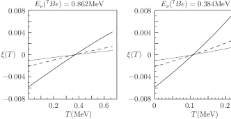
Figure 12: The ratio of electron recoil spectrum from $0.862$-MeV and $0.384$-MeV ${}^{7}Be$ neutrino line to the SM tree-level prediction. The mixing ${\cal U}_{ee}$ is set to unity and $1/R=1.5,2.5,3.5$ TeV for solid, dash and dotted curves respectively.

For neutrino source with continuous energy distribution, the averaged differential scattering cross section as a function of $T$ is experimentally interesting.

$$\left\langle{d\sigma\over dT}\right\rangle_{T}=\int^{E_{max}}_{E_{min}}dE_{\nu}\lambda(E_{\nu}){d\sigma\over dT}$$ (111)

where $\lambda(E_{\nu})$ is the probability distribution in terms of neutrino energy. The minimum energy of incident neutrino to give electron recoil energy $T$ is

$$E_{min}={T+\sqrt{T(T+2m_{e})}\over 2}.$$ (112)

Similarly, we define

$$\left\langle{d\sigma\over dT}\right\rangle_{T}\equiv\left\langle{d\sigma_{\rm SM}\over dT}\right\rangle_{T}(1+\bar{\xi}(T))\,.$$ (113)

For water Cerenkov type experiments, the dominate solar neutrinos come from the decay process ${}^{8}B\rightarrow\,^{7}Be^{*}+e^{+}+\nu_{e}$ and the small fraction of $hep$ neutrinos from process ${}^{3}He+p\rightarrow\,^{4}He+e^{+}+\nu_{e}$ can be ignored. We give plots on $\bar{\xi}(T)$ for solar ${}^{8}B$ neutrinos in Fig.13 with the $\lambda(E_{\nu})$ adopted form BahcallB . In the best case scenario, i.e. low $1/R$ and maximal mixing, the deviation could reach level of a percent at low recoil energies. This is comparable to the radiative correction suppression at high recoil energies Bahcall:1995mm . When the mixing vanishes, vector bilepton $V^{\pm}$ has no contribution, we are left with the effect from KK $W$ and $Z$ which gives a roughly constant correction $\bar{\xi}(T)\sim\{-0.0005,-0.0002,-0.0001\},\{0.0014,0.0005,0.0003\}$ for $\nu_{e,\mu}-e$ scattering with $1/R=\{1.5,2.5,3.5\}$ TeV respectively. Note that unitarity condition requires $|{\cal U}_{ee}|^{2}+|{\cal U}_{\mu e}|^{2}+|{\cal U}_{\tau e}|^{2}=1$, so the bilepton effects always show up in some flavor combination.

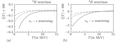
Figure 13: The recoil spectrum distortion for (a) $\nu_{e}-e$ and (b) $\nu_{\mu}-e$ scattering from solar ${}^{8}B$ neutrino. The mixing $|{\cal U}_{ee,\mu e}|$ is set to unity for (a,b) and $1/R=1.5,2.5,3.5$ TeV for solid, dash and dotted curves respectively.

VIII Conclusion

We have carefully gone through the possible phenomenology of the 5D orbifold $SU(3)_{W}$ GUT model SU3:triumf . The RGEs and unification has been examined in section III, we found that the compactification scale, $1/R$, is around $1.5-5$ TeV which makes phenomenology interesting.

Due to KK number conservation and tree-level mass relations, the decays of KK excitations are dominated by the final states constituted by brane fermions, i.e. the SM fermions, only. At the tree level, this results in a universal prediction of $\Gamma^{KK}_{n}/M^{KK}_{n}\sim 2\Gamma^{SM}/M_{SM}$ for any KK state and level $n$.

The scalar and vector bileptons come naturally with the $SU(3)_{W}$ gauge symmetry, which induces many testable signatures. The couplings between vector bilepton and leptons are modulated by a CKM like unitary mixing matrix , ${\cal U}$, which is controlled by the details of Yukawa sector. In principle, the ${\cal U}$ can give CP violation in the lepton sector which will be addressed elsewhere. Lepton flavor changing processes stem from non-diagonal ${\cal U}$. Among them, we found that the muonium-antimuonium conversion and $\mu\rightarrow 3e$ experiments put the most stringent constraints on the model. The existing constraints already hint at Yukawa couplings must exhibit some special patterns in order that the model remains viable. We gave two extreme examples to demonstrate how the Yukawa patterns help to ameliorate the constraints from experimental. Alternatively, if the main features of the model were to be confirmed knowledge of Yukawa structure will be obtained from precise flavor violating experiments.

Now we summarize the possible signatures of this model:

1. For very low energy, the neutrino-electron scattering will receive corrections from all kinds of KK excitation. These corrections can be as large as the SM quantum corrections but with opposite trends. Neutrino flavor changing scattering clearly indicate new physics beyond SM but the rate is estimated to be too small for detection.

2. With the linear colliders with $\sqrt{s}<1/R$, say $\sim 500$ GeV, the Bhabha and Møller scattering spectrum can be very different from SM. The smoking gun evidence for bileptons will be flavor changing scattering, $e^{-}e^{-}\rightarrow e^{-}\mu^{-},\tau^{-}\mu^{-},\cdots$ and $e^{+}e^{-}\rightarrow e^{+}\mu^{-},\mu^{+}\mu^{-},\cdots$. The rates depend on the off-diagonal entities of ${\cal U}$ which cannot be predicted in this model.

3. For a linear collider with $\sqrt{s}$ around $1/R$, there will be strong resonance enhancement for $e^{-}e^{-}\rightarrow\mu^{-}\mu^{-},\tau^{-}\tau^{-}$ and $e^{+}e^{-}\rightarrow e^{+}\mu^{-}$ and so on. This are unmistakable signals of vector bilepton.

4. With a multi-TeV linear collider that has energy reach of $\sqrt{s}\sim 2/R>3$ TeV, we can see the direct productions of gauge exotic bosons: $e^{+}e^{-}\rightarrow U^{\pm 2}U^{\mp 2},V^{\pm}V^{\mp}$ and $e^{+}e^{-}\rightarrow W_{0}^{\pm}W_{1}^{\mp}$. The extra $W_{1}W_{0}$ channel will distinguish this 5D model from the 4D models with bileptons. And at the same effective $\sqrt{s}$ range, the hadron collider can produce single $W_{1}^{\pm}$ KK mode but not $V^{\pm}$ KK mode.

Hopefully these can be seen in the next generation of experiments.

Appendix A KK decomposition and KK number conservation law

On the $S_{1}/(Z_{2}\times Z^{\prime}_{2})$ orbifold, the bulk fields can be decomposed in terms of eigen-modes( $n>0$),

$$\phi^{++}_{n}(y) = {1\over\sqrt{\pi R}}\cos\frac{2ny}{R}$$ (114)

$$\phi^{+-}_{n}(y) = {1\over\sqrt{\pi R}}\cos\frac{(2n-1)y}{R}$$ (115)

$$\phi^{-+}_{n}(y) = {1\over\sqrt{\pi R}}\sin\frac{(2n-1)y}{R}$$ (116)

$$\phi^{--}_{n}(y) = {1\over\sqrt{\pi R}}\sin\frac{2ny}{R}$$ (117)

and the only zero mode $\phi^{++}_{0}(y)=1/\sqrt{2\pi R}$. To simplify the notation, we will use $\{e^{n}_{1},o^{n}_{1},o^{n}_{2},e^{n}_{2}\}$ to denote the $n-$th modes of $\phi^{++}$, $\phi^{+-}$, $\phi^{-+}$ and $\phi^{--}$ respectively. The physical space is $y\in[0,\pi R/2]$. But the integration has to be carried over the whole space $y\in[0,2\pi R]$ such that they form a orthonormal basis:

$$\langle e^{n}_{1}|e^{m}_{1}\rangle=\langle e^{n}_{2}|e^{m}_{2}\rangle=\langle o^{n}_{1}|o^{m}_{1}\rangle=\langle o^{n}_{2}|o^{m}_{2}\rangle=\delta_{m,n}\,,$$

$$\langle e^{n}_{1}|e^{m}_{2}\rangle=\langle e^{n}_{1}|o^{m}_{1}\rangle=\langle e^{n}_{1}|o^{m}_{2}\rangle=0\,,$$

$$\langle e^{n}_{2}|o^{m}_{1}\rangle=\langle e^{n}_{2}|o^{m}_{2}\rangle=\langle o^{n}_{1}|o^{m}_{2}\rangle=0\,.$$

It can be found that

$$e_{1}^{n}e_{1}^{m}={e_{1}^{n+m}+e_{1}^{n-m}\over 2},\,e_{2}^{n}e_{2}^{m}={e_{1}^{n-m}-e_{1}^{n+m}\over 2},$$

$$o_{1}^{n}o_{1}^{m}={e_{1}^{n+m-1}+e_{1}^{n-m}\over 2},o_{2}^{n}o_{2}^{m}={e_{1}^{n-m}-e_{1}^{n+m-1}\over 2},$$

$$e_{1}^{n}e_{2}^{m}={e_{2}^{n+m}-e_{2}^{n-m}\over 2},\,e_{1}^{n}o_{1}^{m}={o_{1}^{n+m}+o_{1}^{n-m+1}\over 2},$$

$$e_{1}^{n}o_{2}^{m}={o_{2}^{n+m}-o_{2}^{n-m+1}\over 2},\,e_{2}^{n}o_{1}^{m}={o_{2}^{n+m}+o_{2}^{n-m+1}\over 2},$$

$$e_{2}^{n}o_{2}^{m}={-o_{1}^{n+m}+o_{1}^{n-m+1}\over 2},o_{1}^{n}o_{2}^{m}={e_{2}^{n+m-1}-e_{2}^{n-m}\over 2}.$$

Note that the KK number conservation rule now is

$$2n^{e}_{1}\pm 2n^{e}_{2}\pm\cdots\pm(2n^{o}_{1}-1)\pm(2n^{o}_{2}-1)\pm\cdots=0$$ (118)

where $n^{e}_{i}$($n^{o}_{i}$) is the KK number of the $i-$th even(odd) mode. This is different from the $S_{1}/Z_{2}$ case. Taking 3 bulk fields (with KK number $l,m,n$) interaction as an example, besides the usual $m\pm n\pm l=0$ rule there is another $m\pm n\pm l=1$ rule for two odd-modes fuse with one even-mode. It is easily understood since the transformation of $Z_{2}$ followed by $Z_{2}^{\prime}$ is equal to the translation, $y\rightarrow y+2\pi R$, which will modify KK number by one.

Appendix B Some handy formulas

Here we collect some useful identities for calculation. The charge conjugation is defined as $\psi^{\mathbf{c}}=C\bar{\psi}^{T}$ and the matrix $C$ satisfies:

$$C^{\dagger}C=1,\,C^{T}=-C,\,C\gamma^{T}_{\mu}C^{-1}=-\gamma_{\mu}$$ (119)

and also

$$C\sigma_{\mu\nu}^{T}C^{-1}=\sigma_{\mu\nu},\,C\gamma_{5}^{T}C^{-1}=\gamma_{5},\,C(\gamma_{\mu}\gamma_{5})C^{-1}=\gamma_{\mu}\gamma_{5}\,.$$ (120)

We use the representation : $C=-i\gamma^{2}\gamma^{0}$. Also $\bar{\psi^{\mathbf{c}}}=-\psi^{T}C^{-1}$, and the helicity projections are $P_{L/R}=(1\mp\gamma^{5})/2$. The following relations can be derived

$$\bar{\psi^{\mathbf{c}}_{1}}P_{L/R}\psi_{2}=\bar{\psi^{\mathbf{c}}_{2}}P_{L/R}\psi_{1}\,,$$ (121)

$$\bar{\psi_{1}}P_{L/R}\psi^{\mathbf{c}}_{2}=+\bar{\psi_{2}}P_{L/R}\psi_{1}^{\mathbf{c}}\,,$$ (122)

$$\bar{\psi_{1}}\gamma^{\mu}P_{L/R}\psi^{\mathbf{c}}_{2}=-\bar{\psi_{2}}\gamma^{\mu}P_{R/L}\psi^{\mathbf{c}}_{1}\,,$$ (123)

$$\bar{\psi_{1}^{\mathbf{c}}}\gamma^{\mu}P_{L/R}\psi_{2}=-\bar{\psi_{2}^{\mathbf{c}}}\gamma^{\mu}P_{R/L}\psi_{1}\,,$$ (124)

$$\bar{\psi_{1}^{\mathbf{c}}}P_{L/R}\psi_{2}^{\mathbf{c}}=\bar{\psi_{2}}P_{L/R}\psi_{1}\,,$$ (125)

$$\bar{\psi_{1}^{\mathbf{c}}}\gamma^{\mu}P_{L/R}\psi_{2}^{\mathbf{c}}=-\bar{\psi_{2}}\gamma^{\mu}P_{R/L}\psi_{1}\,,$$ (126)

$$(\bar{\psi_{1}}P_{L}\psi_{3})(\bar{\psi_{2}}P_{R}\psi_{4})=$$

$$-\frac{1}{2}(\bar{\psi_{1}}\gamma^{\mu}P_{R}\psi_{4})(\bar{\psi_{2}}\gamma_{\mu}P_{L}\psi_{3})\,,$$ (127)

$$(\bar{\psi_{1}}\gamma^{\mu}P_{L/R}\psi_{3})(\bar{\psi_{2}}\gamma_{\mu}P_{L/R}\psi_{4})=$$

$$(\bar{\psi_{1}}\gamma^{\mu}P_{L/R}\psi_{4})(\bar{\psi_{2}}\gamma_{\mu}P_{L/R}\psi_{3})\,.$$ (128)

Appendix C Triple gauge coupling

The Feynman rules for triple gauge boson coupling are summarized in the following table.

a	$A$	$A$	$A$	$Z$	$Z$	$Z$	$W^{-}$
b	$W^{+}$	$V^{+}$	$U^{+2}$	$W^{+}$	$V^{+}$	$U^{+2}$	$U^{+2}$
c	$W^{-}$	$V^{-}$	$U^{-2}$	$W^{-}$	$V^{-}$	$U^{-2}$	$V^{-}$
$d_{abc}$	$s_{W}$	$s_{W}$	$2s_{W}$	$c_{W}$	$-{1\over 2c_{W}}$	${1-4s_{W}^{2}\over 2c_{W}}$	$\frac{1}{\sqrt{2}}$

Where $a,b,c$ denote the gauge boson species and $d_{abc}$ can be easily determined by group structure. The indices $l,m,n$ collectively represent their corresponding KK numbers and $(Z_{2},Z^{\prime}_{2})$ parity. $\kappa$ is totally symmetric and is determined by

$$\kappa_{lmn}=\sqrt{2\pi R}\int^{2\pi R}_{0}dy\phi_{l}(y)\phi_{m}(y)\phi_{n}(y).$$ (129)

For example, $\kappa_{0_{++},n_{+-},n_{+-}}=\kappa_{0_{++},n_{++},n_{++}}=1$, and $\kappa_{2n_{++},n_{++},n_{++}}=1/\sqrt{2}$. In fact, $\kappa=1$ when any one of the three is a zero mode and all the other allowed combinations which respect KK number conservation and $Z_{2}\times Z^{\prime}_{2}$ parity give $\pm 1/\sqrt{2}$.

References

- (1) S. Weinberg, Phys. Rev. D 5, 1962 (1972).
- (2) E. J. Konopinski and H. M. Mahmoud, Phys. Rev. 92 (1953) 1045.
- (3) P. H. Frampton, Phys. Rev. Lett. 69, 2889 (1992). F. Pisano and V. Pleitez, Phys. Rev. D 46, 410 (1992) [arXiv:hep-ph/9206242].
-
(4)
L. J. Hall and Y. Nomura,
Phys. Lett. B 532, 111 (2002)
[arXiv:hep-ph/0202107].
T. j. Li and W. Liao, Phys. Lett. B 545, 147 (2002) [arXiv:hep-ph/0202090].
S. Dimopoulos and D. E. Kaplan, Phys. Lett. B 531, 127 (2002) [arXiv:hep-ph/0201148].
S. Dimopoulos, D. E. Kaplan and N. Weiner, Phys. Lett. B 534, 124 (2002) [arXiv:hep-ph/0202136].
- (5) Y. Fukuda et al. [Super-Kamiokande Collaboration], Phys. Rev. Lett. 8119981562 [hep-ex/9807003].
- (6) Q. R. Ahmad et al. [SNO Collaboration], Phys. Rev. Lett. 892002011301 [nucl-ex/0204008].
- (7) K. Eguchi et al. [KamLAND Collaboration], Phys. Rev. Lett. 902003021802 [hep-ex/0212021].
- (8) C. L. Bennett et al., [astro-ph/0302207].
-
(9)
A. Zee,
Phys. Lett. B 93, 389 (1980)
[Erratum-ibid. B 95(1980)461];
A. Zee, Phys. Lett. B 161, 141 (1985). - (10) C. H. Chang, W. F. Chang and J. N. Ng, Phys. Lett. B 558, 92 (2003) [arXiv:hep-ph/0301271].
- (11) W. F. Chang and J. N. Ng, JHEP 0310, 036 (2003) [arXiv:hep-ph/0308187].
-
(12)
K. R. Dienes, E. Dudas and T. Gherghetta,
Nucl. Phys. B 537, 47 (1999)
[arXiv:hep-ph/9806292];
K. R. Dienes, E. Dudas and T. Gherghetta, Phys. Lett. B 436, 55 (1998) [arXiv:hep-ph/9803466];
K. R. Dienes, E. Dudas and T. Gherghetta, [arXiv:hep-th/0210294]. - (13) J. N. Ng, [arXiv:hep-ph/0311352].
- (14) For a comprehensive review of bileptons, see F. Cuypers and S. Davidson, Eur. Phys. J. C 2, 503 (1998) [arXiv:hep-ph/9609487], and references therein.
- (15) J. N. Ng, Phys. Rev. D 31, 464 (1985). D. Ng, Phys. Rev. D 49, 4805 (1994) [arXiv:hep-ph/9212284]. N. Lepore, B. Thorndyke, H. Nadeau and D. London, Phys. Rev. D 50, 2031 (1994) [arXiv:hep-ph/9403237]. F. Cuypers and M. Raidal, Nucl. Phys. B 501, 3 (1997) [arXiv:hep-ph/9704224]. P. H. Frampton and A. Rasin, Phys. Lett. B 482, 129 (2000) [arXiv:hep-ph/0002135].
- (16) P. H. Frampton and D. Ng, Phys. Rev. D 45, 4240 (1992). V. Pleitez, Phys. Rev. D 61, 057903 (2000) [arXiv:hep-ph/9905406].
- (17) B. Dion, T. Gregoire, D. London, L. Marleau and H. Nadeau, Phys. Rev. D 59, 075006 (1999) [arXiv:hep-ph/9810534].
-
(18)
J. C. Pati and A. Salam,
Phys. Rev. D 10, 275 (1974).
R. N. Mohapatra and J. C. Pati, Phys. Rev. D 11, 2558 (1975).
G. Senjanovic and R. N. Mohapatra, Phys. Rev. D 12, 1502 (1975).
P. H. Frampton and B. H. Lee, Phys. Rev. Lett. 64, 619 (1990). -
(19)
K. R. Dienes, E. Dudas and T. Gherghetta,
Nucl. Phys. B 537, 47 (1999)
[arXiv:hep-ph/9806292].
J. Papavassiliou and A. Santamaria, Phys. Rev. D 63, 125014 (2001) [arXiv:hep-ph/0102019].
W. F. Chang, I. L. Ho and J. N. Ng, Phys. Rev. D 66, 076004 (2002) [arXiv:hep-ph/0203212].
A. Muck, A. Pilaftsis and R. Ruckl, Phys. Rev. D 65, 085037 (2002) [arXiv:hep-ph/0110391]. - (20) W.J. Marciano, Phys. Rev. D 60 , 093006 (1999)
-
(21)
K. Hagiwara et al. [Particle Data Group Collaboration],
Phys. Rev. D 66 (2002) 010001.
W. Fetscher, H. J. Gerber and K. F. Johnson, Phys. Lett. B 173, 102 (1986). -
(22)
C. Athanassopoulos et al. [LSND Collaboration],
Phys. Rev. C 54, 2685 (1996)
[arXiv:nucl-ex/9605001].
C. Athanassopoulos et al. [LSND Collaboration], Phys. Rev. Lett. 77, 3082 (1996) [arXiv:nucl-ex/9605003].
A. Aguilar et al. [LSND Collaboration], Phys. Rev. D 64, 112007 (2001) [arXiv:hep-ex/0104049]. -
(23)
G. Feinberg and S. Weinberg,
Phys. Rev. Lett. 6, 381(1961);
Phys. Rev. 123, 1439(1961).
D. Chang and W. Y. Keung, Phys. Rev. Lett. 62, 2583 (1989).
K. Horikawa and K. Sasaki, Phys. Rev. D 53, 560 (1996) [arXiv:hep-ph/9504218].
H. Fujii, Y. Mimura, K. Sasaki and T. Sasaki, Phys. Rev. D 49, 559 (1994) [arXiv:hep-ph/9309287].
W. S. Hou and G. G. Wong, Phys. Rev. D 53, 1537 (1996) [arXiv:hep-ph/9504311]. - (24) L. Willmann et al., Phys. Rev. Lett. 82, 49 (1999) [arXiv:hep-ex/9807011].
- (25) G. ’t Hooft, Phys. Lett. B 37 (1971) 195.
- (26) J. N. Bahcall, M. Kamionkowski and A. Sirlin, Phys. Rev. D 51, 6146 (1995) [arXiv:astro-ph/9502003].
- (27) J. N. Bahcall, Neutrino Astrophysics,Cambridge University Press, 1990.