The hadronic potential at short distance

Abstract

A fictitious discussion is taken as a point of origin to present novel physical insight into the nature of gauge theory and the potential energy of QCD and QED at short distance. Emphasized is the considerable freedom in the cut-off function which eventually can modify the Coulomb potential of two charges at sufficiently small distances. Emphasized is also that the parameters of the regularization function (the “cut-off scale”) should not be driven to infinity but kept constant in line with the modern interpretation of renormalization theory. The paper restricts to general aspects. The technical paraphernalia and the comparison with experiment are shifted to a sequence of 4 subsequent stand-alone and sufficiently small papers to be published immediatelely hereafter.

1 Introduction: Highlights of a discussion

In the aftermath of recent conference contributions Pau03a , I had to survive serious discussions whose highlights should be interesting for a larger audience. In a way, the arguments of a fictitious anonymous represent the state of the art public opinion of the high energy physics community. I let play him the role of the devils advocate. Here are some of his points:

1. QCD interactions at short distances are scale invariant – up to the logarithmic asymptotic freedom corrections predicted from the running coupling. This near conformal scaling of QCD is well tested in quark-quark scattering and other jet physics measurements at colliders.

2. Certainly $\Lambda_{QCD}$ sets the scale of the hadronic parameters. It is relevant to QCD interactions at large distances.

3. Evidence is accumulating that the running coupling – as defined from the Landau gauge gluon propagator or observables – is well regulated at small $Q^{2}$. Some relevant papers are vonSmekal:1997is ; Howe:2002rb ; Mattingly:1994 ; Brodsky:2002nb .

4. It might be worthwhile to look at the Fourier transform of ${\alpha_{s}(Q^{2})}/{Q^{2}}$ where $\alpha_{s}(Q^{2})$ is the Shirkov form, as given for example in the paper Baldicchi:2002 .

5. Pauli uses a cut-off $\lambda$ to motivate a modification of the short distance $r\to 0$ QCD interaction. — Let us compare the Yukawa ${1}/{(Q^{2}+\lambda^{2})}$ and Coulomb ${1}/{Q^{2}}$ interactions. They are identical at large $Q^{2}$. — Their respective Fourier transforms potentials are the ${\mathrm{e}^{-\lambda r}}/{r}$ and $1/r$. They are identical at short distances $r\to 0$!

Here is a summary of my points:

1. Relating large momentum transfers to short distances is often only a figure of speech. The relation between a scattering amplitude $T(Q^{2})$ and an interaction $V(r)$ is a highly non-trivial matter.

2. Colliders measure the scattering amplitude $\alpha_{s}(Q^{2})/Q^{2}$ at large $Q^{2}$. The interaction is the Fourier transform of ${\alpha_{s}(Q^{2})}/{Q^{2}}$, all $Q^{2}$ are needed, and not only the large ones.

3. We should be more careful about our terms of speaking, and specify by operational prescriptions what we mean by ‘interaction’ and/or ‘potential’.

4. The $q\bar{q}$ potential at short distance simply cannot go like $\alpha_{s}/r$, whatever the numerical value of the strong coupling ‘constant’ $\alpha_{s}$ is.

5. The literature has too many $\Lambda$’s! The same mathematical symbol refers to completely different physics.

In this short note, I will work out to some detail why and to which extent I will arrive at conclusions different from the public opinion.

I use this opportunity as the port of entry for presenting novel insights on the nature of the gauge field interaction at short distance. In Pau03b I will present a possible solution to the problem of the non perturbative renormalization in a gauge theory. In Pau03c , the technical details of the fine and hyperfine interaction on the light cone will be discussed. In Pau03d and Pau03e I will calculate the ground state masses and mass spectra of all flavor off diagonal pseudo scalar and pseudo vector mesons, analytically, for a linear and for a quadratic potential.

2 Taking Fourier transforms

Collider physics is consistent with asymptotic freedom,

$$\alpha_{s}(Q^{2})=\frac{4\pi}{\beta_{0}\mathrm{ln}(Q^{2}/\Lambda^{2}_{QCD})}\,,$$ (1)

at sufficiently large $Q^{2}$, with the famous $\beta_{0}=11n_{c}-2n_{f}$. What is its Fourier transform?

Let us be specific. Consider

$$V(r) = -\frac{1}{2\pi^{2}}\int\!d^{3}q\;\frac{\alpha_{c}(q^{2})}{q^{2}}\;\mathrm{e}^{-i\vec{q}\vec{r}},$$ (2)

where $\alpha_{c}(q^{2})=\frac{4}{3}\alpha_{s}(q^{2})$ given by Eq.(1) with the Feynman four momentum transfer $Q^{2}$ substituted by the three momentum transfer $q^{2}=(\vec{k}-\vec{k}^{\prime})^{2}$. Integrating over the angles gives

$$V(r) = -\frac{1}{\pi}\int_{0}^{\infty}\!dq\;q^{2}\;\frac{\alpha_{c}(q^{2})}{q^{2}}\;\int_{-1}^{+1}\!\!\!\!d(\cos\theta)\;\mathrm{e}^{-iqr\cos\theta}$$ (3)

$$= -\frac{2}{\pi}\int_{0}^{\infty}\!dq\;{\alpha_{c}(q^{2})}\;\frac{\sin qr}{qr}.$$

But this integral does not exist!

The problem is as absent for short distances $r\to 0$, as long as $\alpha_{c}(q^{2})$ is integrable. The available ‘effective’ $\alpha_{c}(q^{2})$ in vonSmekal:1997is ; Howe:2002rb ; Mattingly:1994 ; Brodsky:2002nb may or may not allow for $\int_{0}\!dq\;{\alpha_{c}(q^{2})}$.

The problem resides at the upper limit. A Fourier transform of a function is defined only if its limes superior exists, that is, it exists only if

$$\int^{\infty}\!\frac{dq}{q}\;{\alpha_{c}(q^{2})}\;$$

is a well defined expression. But Eq.(3) it not well defined. It diverges at the upper limit, since:

$$\int\!\frac{dq}{q\ln q}=\ln\ln q\,.$$ (4)

Knowing that asymptotic freedom is too weak a regulator, I have not even attempted in the past, to carry out point 4 of the advocate. Baldicchi and Prosperi Baldicchi:2002 also know about the problem, but they veil it by inserting a linear potential as a regulator, by hand and out of desperation.

One concludes that the integral, Eq.(2), must be regulated. What are possible alternatives?

Cutting-off at the upper limit à la $\int^{q_{0}}\!dq$ makes not much sense sense. A sharp cut-off with the step function $R(q)=\Theta(q^{2}-\lambda^{2})$ generates uncontrollable oscillations. A soft regulator function, as for example

$$R(q)=\frac{\lambda^{2}}{\lambda^{2}+q^{2}}\,,$$ (5)

satisfies however all important requirements, among them $R(q)\Longrightarrow 1$ for $\lambda\Longrightarrow\infty$ and no extra physical dimensions. It is dimensionless.

In consequence one replaces Eq.(2) by

$$V(r) = -\frac{1}{2\pi^{2}}\int\!d^{3}q\;\frac{\alpha_{c}(q^{2})}{q^{2}}\;R(q)\;\mathrm{e}^{-i\vec{q}\vec{r}},$$ (6)

and Eq.(3) by

$$V(r) = -\frac{2}{\pi}\int_{0}^{\infty}\!dq\;{\alpha_{c}(q^{2})}\;R(q)\;\frac{\sin qr}{qr}.$$ (7)

One faces now a well defined mathematical problem.

But one faces another problem: The integrand behaves like:

$$\frac{4\pi}{\beta_{0}\mathrm{ln}(q^{2}/\Lambda^{2}_{QCD})}\;\frac{\lambda^{2}}{\lambda^{2}+q^{2}}\;\frac{\sin qr}{qr}.$$

The large q behavior is dominated completely by the regulator and the rapid oscillations of the sine function. As compared to them, the logarithm is hyper slowly varying. A mathematician would treat the problem by replacing the slowly varying term by a constant $\alpha^{\prime}_{c}$ and take it out of the integral. (He would call this step the saddle point approximation.) He thus would get

$$V(r) = -\frac{2\alpha^{\prime}_{c}}{\pi}\int_{0}^{\infty}\!dq\;R(q)\;\frac{\sin qr}{qr}$$ (8)

$$= \displaystyle\alpha^{\prime}_{c}\Big{[}\frac{\mathrm{e}^{-\lambda r}}{r}-\frac{1}{r}\Big{]}\,.$$ (9)

Here are the Coulomb’s and Yukawas which the advocate refers to in his point 5. He is right, of course, in stating that they are identical at short distances $r\to 0$.

The notion ‘identical’ is misleading: The leading singularities cancel, but still $V(r\to 0)$ is non-zero. The systematic expansion for short distances rather gives

$$V(r) = -a+b\;r\,,$$ (10)

plus possible higher terms to which I shall come below.

The numerical values of $a$ and $b$ are less important for the argument. But for completeness, here they are:

$$a = \alpha^{\prime}_{c}\;\lambda\,,$$ (11)

$$b = \alpha^{\prime}_{c}\;\lambda^{2}/2\,.$$ (12)

The considerations, which lead to Eq.(10), also highlight another aspect. The only piece of non ambiguous experimental information is the coupling constant at very high momentum transfer: The ‘running’ constant at the $Z$ mass $M_{Z}\simeq 91.2\mbox{ GeV}$. Its experimental value is $\alpha_{s}(M_{Z})\simeq 0.118$. The coupling constant $\alpha_{s}^{\prime}=\alpha_{s}(q_{0})$ can thus be taken at comparatively large values of $q_{0}$. The argument of $\alpha^{\prime}_{s}=\alpha_{s}(Q=0)$ in Pau03a is false, since $\alpha^{\prime}_{s}=\alpha_{s}(q_{0})$, but the preliminary value

$$\alpha^{\prime}_{s}=0.1695\,,$$ (13)

taken from Pau03a , is a useful first guess subject to later re adjustment. The numerical value of $\alpha^{\prime}_{s}$ is comparatively small, much smaller in any case than the often quoted value $\alpha^{\prime}_{s}=0.7$. Setting the scale, like in Pau03a ,

$$\lambda=200\mbox{ MeV}\,,$$ (14)

determines all parameters.

The above argument shows that the asymptotic scale $\Lambda_{QCD}$ in Eq.(1) is conceptually different from the regularization scale $\lambda$ in Eq.(5). It is $\lambda$, not $\Lambda_{QCD}$, which sets the scale of the problem – contrary to point 2 of the advocate. The confusion arises since both scales are often quoted with the same numerical value of about $200\mbox{ MeV}$, corresponding to a length scale of about $1\mbox{ fm}$.

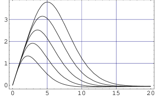
Figure 1: The dimensionless Coulomb potential $W_{N}(y;0,1,0)$ is plotted versus the radius parameter $y=\lambda r$. The different $N=4,5,6,7,8$ are drawn by the curves from bottom to top.

3 The generalized regulator function

It should be emphasized that the limit $\lambda\to\infty$ may not be taken in Eq.(9): For $\lambda\to\infty$, one is back to the undefined problem of Eq.(3).

The same conclusion will also be reached with the renormalization group equations Pau03b . The renormalization group equations Pau03b require also that the regulator function has well defined derivatives with respect to $\lambda$. This excludes the step function of the sharp cut-off from the class of admitted regulator functions. The theta function is a distribution with only ill defined derivatives. Having understood these essentials, one can phrase things in a very simple way.

Do the above statements imply that the ‘soft’ regulator in Eq.(5) is the only one admitted? — Of course not.

In fact, one has a large class of ‘generalized regulator functions’ Pau03a :

$$R(q)=\left[1+\sum_{n=1}^{N}(-1)^{n}s_{n}\lambda^{n}\frac{\partial^{n}}{\partial\lambda^{n}}\right]\frac{\lambda^{2}}{\lambda^{2}+q^{2}}\,.$$ (15)

The partials $\lambda^{n}\,\partial^{n}/\partial\lambda^{n}$ are dimensionless and independent of a change in $\lambda$. The arbitrarily many coefficients $s_{1},\dots,s_{N}$ are renormalization group invariants and, as such, subject to be determined by experiment.

The generalized regulator yields immediately the generalized Coulomb potential

$$V(r) = -\frac{\alpha_{c}}{r}\Big{[}1+\sum_{n=1}^{N}(-1)^{n}s_{n}\lambda^{n}\frac{\partial^{n}}{\partial\lambda^{n}}\Big{]}\Big{(}1-\mathrm{e}^{-\lambda r}\Big{)}$$ (16)

$$= \phantom{-}\frac{\alpha_{c}}{r}\Big{[}-1+\mathrm{e}^{-{\lambda r}}\sum_{n=0}^{N}s_{n}({r\lambda})^{n}\Big{]},$$

with $s_{0}\equiv 1$. This result illustrates an other important point: The power series in front of the exponential are nothing but a spelled out version of Laguerre polynomials. Laguerre polynomials are a complete set of functions. Eq.(16) is thus potentially able to reproduce an arbitrary function of $r$. The description in terms of a generating function, as in Eqs.(15) or (16), is therefore complete.

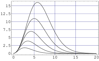
Figure 2: The dimensionless Coulomb potential $W_{N}(y;0,0,1)$ is plotted versus the radius parameter $y=\lambda r$. The different $N=4,5,6,7,8$ are drawn by the curves from bottom to top.

The large number of parameter in Eq.(16) can be controlled by the following construction: The coefficients $s_{n}$ in Eq.(16) are expressed in terms of only three parameters $a$, $b$, and $c$, by

$$s_{n}=\frac{1}{n!}+\frac{a}{(n-1)!}+\frac{b}{(n-2)!}+\frac{c}{(n-3)!}\,.$$ (17)

The first few coefficients are then explicitly

$$\begin{array}[]{rc rc rc rc rc rc }s_{0}&=&1&,&\\ s_{1}&=&1&+&a&,&\\ s_{2}&=&\frac{1}{2}&+&a&+&b&,&\\ s_{3}&=&\frac{1}{6}&+&\frac{a}{2}&+&b&+&c&,&\\ s_{4}&=&\frac{1}{24}&+&\frac{a}{6}&+&\frac{b}{2}&+&c&.&\end{array}$$ (23)

As a consequence, the dimensionless Coulomb potential depends on $r$ only through the dimensionless combination $y=\lambda r$:

$$W_{N}(y;a,b,c)=\frac{V(r)}{\alpha_{c}\lambda}=\frac{1}{y}\Big{(}-1+\mathrm{e}^{-y}\sum_{n=0}^{N}s_{n}y^{n}\Big{)}\,.$$ (24)

In the near zone, it is a quadratic function of $y$,

$$W_{N}(y;a,b,c)=a+by+cy^{2}\,,$$ (25)

independent of the value of $N$. The remainder starts at most with power $y^{N+1}$. A value of $a=c=0$ and $b=1$ should yield a linear set of functions $W_{N}(y;0,1,0)\simeq y$ in the near zone. As shown in Fig. 1 with the original Mathematica plot, this happens to be true for surprisingly large values of $y$, i.e. not only for $y\ll 1$. The value of $N$ essentially controls the height of a barrier. Similarly, $W_{N}(y;0,0,1)=y^{2}$ generates a set of functions which are strictly quadratic in the near zone. Again, $N$ controls the height of a barrier.

The physical picture which develops is illustrated in Fig. 3. In the far zone, for sufficiently large $r$, the potential energy coincides with the conventional Coulomb potential $-\frac{\alpha_{c}}{r}$. Since the potential is attractive, it can host bound states which are probably those realized in weak binding. In the near zone, for sufficiently small $r$, the potential behaves like a power series $c_{0}+c_{1}r+c_{2}r^{2}$ which potentially can host the bound states of strong coupling, provided the actual parameter values allow for that. In the intermediate zone, the actual potential must interpolate between these two extremes, since Eq.(16) is an analytic function of $r$. Most likely this is done by developing a barrier of finite height, depending on the actual parameter values. The onset of the near and intermediate regimes must occur for relative distances of the quarks, which are comparable to the Compton wave length associated with their reduced mass. If the distance is smaller, one expects deviations from the classical regime by elementary considerations on quantum mechanics, indeed.

4 Conclusions and remaining mysteries

Once the arguments in Sec. 2 are accepted for Quantum Chromodynamics (QCD), one must accept them also for Quantum Electrodynamics (QED). The integral in Eq.(3) for QED diverges even stronger than for QCD. I thus arrive at the incredible conclusion that the potential energy between a muon and an electron is linear (or quadratic!) for sufficiently short distance.

Do I want to overthrow everything? — As a matter of fact: no! The scales are such that the hadronic length scale $R_{H}=\hbar/\lambda c\sim 1\mbox{ fm}$ is very much smaller than the Bohr scale $R_{B}=\hbar/m_{e}c\cdot 1/\alpha\sim 386\cdot 137\mbox{ fm}$. The electron simply ‘does not see’ the details at short distance except for a small perturbation. We know that from the hydrogen atom where the finite size of the proton gives only a small finite size correction.

The second important conclusion is that linear (or quadratic!) confinement can not go on forever. Confinement must be short distance phenomenon, in sharp contrast to the teleological or theological beliefs of the community. The hadronic potential allows for continuous spectra.

The only mystery remaining is that Lattice Gauge Theories and their representatives insist on a singularity at short distance,

$$V(r) = -\frac{\alpha^{\prime}_{c}}{r}+b\;r\neq-a+b\;r\,,$$ (26)

although inherently to the method, Lattice Gauge Theory can not carry out calculations at the singularity $r=0$. The value of the constant $a$ can take arbitrarily large values, but it must be finite, by definition. I have insufficient working knowledge to comment any further on these questions.

“Subtle is the Lord, but nasty is he not.”

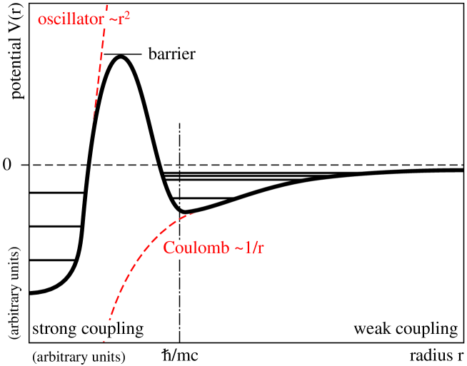
Figure 3: Schematic behavior of the renormalized Coulomb potential, see also the discussion in the text.

- (1) H. C. Pauli, Successful renormalization of a QCD-inspired Hamiltonian. PiHPP, Trieste, 12 - 16 May 2003; arXiv:hep-ph/0310294. NUPP with CEBAF, Dubrovnik, 26 - 31 May, 2003. Light-cone meeting, Durham, 5 - 9 August, 2003.
- (2) L. von Smekal, R. Alkofer and A. Hauck, The infrared behavior of gluon and ghost propagators in Landau gauge QCD, Phys. Rev. Lett. 79, 3591 (1997).
- (3) D. M. Howe and C. J. Maxwell, All-orders infra-red freezing of R(e+e-) in perturbative QCD, Phys. Lett. B 541, 129 (2002); see also arXiv:hep-ph/0303163.
- (4) A. C. Mattingly and P. M. Stevenson, Optimization of R(e+e-) and ’freezing’ of the QCD couplant at low energies, Phys. Rev. D 49, 437 (1994).
- (5) S. J. Brodsky, S. Menke, C. Merino and J. Rathsman, On the behavior of the effective QCD coupling at low scales, Phys. Rev. D 67, 055008 (2003).
- (6) M. Baldicchi, G. M. Prosperi, Infrared behavior of the running coupling constant and bound states in QCD, Phys. Rev. D 66, 074008 (2002).
- (7) H. C. Pauli, Possible solution to the problem of the non perturbative renormalization in a gauge theory (II), arXiv:hep-ph/0312xxx.
- (8) H. C. Pauli, On the fine and hyperfine interaction on the light cone (III), arXiv:hep-ph/0312xxx.
- (9) H. C. Pauli, A linear potential in a light cone QCD inspired model (IV), arXiv:hep-ph/0312xxx.
- (10) H. C. Pauli, A quadratic potential in a light cone QCD inspired model (V), arXiv:hep-ph/0312xxx.