Nov 2003

Numerical evaluation of the general massive
2-loop 4-denominator self-mass master integral
from differential equations.

M. Caffo^ab, H. Czyż ^c, A. Grzelińska^c and E. Remiddi^ba

• INFN, Sezione di Bologna, I-40126 Bologna, Italy

• Dipartimento di Fisica, Università di Bologna, I-40126 Bologna, Italy

• Institute of Physics, University of Silesia, PL-40007 Katowice, Poland

e-mail: caffo@bo.infn.it
             czyz@us.edu.pl
             grzel@joy.phys.us.edu.pl
             remiddi@bo.infn.it

The differential equation in the external invariant $p^{2}$ satisfied by the master integral of the general massive 2-loop 4-denominator self-mass diagram is exploited and the expansion of the master integral at $p^{2}=0$ is obtained analytically. The system composed by this differential equation with those of the master integrals related to the general massive 2-loop sunrise diagram is numerically solved by the Runge-Kutta method in the complex $p^{2}$ plane. A numerical method to obtain results for values of $p^{2}$ at and close to thresholds and pseudo-thresholds is discussed in details.

——————————-
PACS 11.10.-z Field theory,  PACS 11.10.Kk Field theories in dimensions other than four,
PACS 11.15.Bt General properties of perturbation theory,  PACS 12.20.Ds Specific calculations,
PACS 12.38.Bx Perturbative calculations.

1 Introduction.

Precise measurements of particles properties require that the corresponding theoretical calculations have to include up to (at least) two-loop radiative corrections. In this paper we investigate a fast and flexible numerical method for their accurate evaluation.

A commonly used procedure in modern radiative correction calculations is to express the result as a combination of a limited number of Master Integrals (MI’s), using the integration by parts identities [1]. In this framework, it is necessary to obtain a precise determination of the MI’s, even if the analytical values cannot be obtained due to the large number of different scales occurring in each of the MI’s (internal masses and external momenta or Mandelstam variables), as it happens in electroweak theory.

The general massive 2-loop self-mass diagram has four MI’s related to the sunrise (3-denominator) diagram, only one independent MI related to the 4-denominator diagram, and again only one new MI related to the 5-denominator diagram [2, 3, 4, 5].

Several procedures for a precise numerical evaluation of the MI’s have been and still are investigated, such as multiple expansions [6], numerical integration [6, 7, 8, 9, 10, 11, 12, 13, 14], or difference equations [15].

Another method based on differential equations [16, 17] was proposed in [18], where it was shown how to use Runge-Kutta method [19] to solve numerically the system of linear differential equations in the external invariant $p^{2}$ satisfied by sunrise master integrals.

Figure 1: The general massive 2-loop 4-denominator self-mass diagram.

The method was extended to 2-loop 4-denominator and 5-denominator cases in [20], where it was also suggested how to evaluate numerically the MI’s nearby thresholds and pseudo-thresholds. We give in this paper an accurate implementation of that approach for the sunrise and the 4-denominator MI’s.

In Section 2, the $(n-4)$ expansions of the MI’s are constructed, in Section 3 initial conditions for the differential equations for the Master Integrals (or Master Differential Equations, MDE’s) are discussed. Some results of the program, showing characteristic behaviour of the studied MI’s are presented in Section 4. In Section 5, a method for the numerical evaluation of the MI’s near thresholds and pseudo-thresholds is discussed in detail, while Section 6 is devoted to comparisons with existing results.

Finally, in Section 7, our conclusions on the application of the method to present and further work are presented.

2 The MDE and the expansion in $(n-4)$ of the MI

We use here the following definition of the MI related to the general massive 2-loop 4-denominator self-mass diagram, shown in Fig.1,

$$F_{4}(n,m_{1}^{2},m_{2}^{2},m_{3}^{2},m_{4}^{2},p^{2}) = \frac{\mu^{8-2n}}{((2\pi)^{n-2})^{2}}{\kern 20.0pt}\int d^{n}k_{1}\int d^{n}k_{2}$$ (1)

$${\kern-165.0pt}\frac{1}{(k_{1}^{2}+m_{1}^{2})\ [(p-k_{1})^{2}+m_{4}^{2}]\ (k_{2}^{2}+m_{2}^{2})\ [(p-k_{1}-k_{2})^{2}+m_{3}^{2}]}\ ,$$

where integration is performed in $n-$dimensional Euclidean space.

Wherever necessary to avoid ambiguities, the usual imaginary displacements in the masses $m_{i}^{2}\to m_{i}^{2}-i\epsilon$, where $\epsilon$ is an infinitesimal positive number, are understood. The arbitrary mass scale $\mu$ accounts for the continuous value of the dimensions $n$. In numerical calculations, we choose $\mu=m_{1}+m_{2}+m_{3}$, one of the natural scales of the problem, corresponding to the 3-body threshold, while for simplicity in all analytic formulae we put $\mu=1$. To recover results for arbitrary $\mu$, one has to substitute $m_{i}\to{m_{i}}/{\mu}$ and $p^{2}\to{p^{2}}/{\mu^{2}}$.

The master equation reads

$${\kern-30.0pt}R^{2}(-p^{2},m_{1}^{2},m_{4}^{2})\ p^{2}\ \frac{\partial}{\partial p^{2}}F_{4}(n,m_{1}^{2},m_{2}^{2},m_{3}^{2},m_{4}^{2},p^{2})=$$

$$\phantom{+}\frac{n-4}{2}R^{2}(-p^{2},m_{1}^{2},m_{4}^{2})F_{4}(n,m_{1}^{2},m_{2}^{2},m_{3}^{2},m_{4}^{2},p^{2})$$

$$-(n-3)\left[(m_{1}^{2}+m_{4}^{2})p^{2}+(m_{1}^{2}-m_{4}^{2})^{2}\right]F_{4}(n,m_{1}^{2},m_{2}^{2},m_{3}^{2},m_{4}^{2},p^{2})$$

$$+(3p^{2}-m_{1}^{2}+m_{4}^{2})m_{1}^{2}F_{1}(n,m_{1}^{2},m_{2}^{2},m_{3}^{2},p^{2})$$

$$+(p^{2}-m_{1}^{2}+m_{4}^{2})\Biggl{[}\frac{3n-8}{2}F_{0}(n,m_{1}^{2},m_{2}^{2},m_{3}^{2},p^{2})$$

$${\kern 30.0pt}+m_{2}^{2}F_{2}(n,m_{1}^{2},m_{2}^{2},m_{3}^{2},p^{2})+m_{3}^{2}F_{3}(n,m_{1}^{2},m_{2}^{2},m_{3}^{2},p^{2})$$

$${\kern 30.0pt}-\frac{1}{2}(n-2)V(n,m_{2}^{2},m_{3}^{2},m_{4}^{2})\Biggr{]}\ ,$$ (2)

where

$$R^{2}(-p^{2},m_{1}^{2},m_{4}^{2}) = p^{4}+m_{1}^{4}+m_{4}^{4}+2m_{1}^{2}p^{2}+2m_{4}^{2}p^{2}-2m_{1}^{2}m_{4}^{2}$$ (3)

$$= [p^{2}+(m_{1}+m_{4})^{2}][p^{2}+(m_{1}-m_{4})^{2}]\ .$$

The $F_{j}(n,m_{1}^{2},m_{2}^{2},m_{3}^{2},p^{2}),j=0,1,2,3$ are the massive 2-loop sunrise self-mass master amplitudes, discussed in [4] and numerically calculated in [18],

$$F_{j}(n,m_{1}^{2},m_{2}^{2},m_{3}^{2},p^{2}) = \frac{\mu^{8-2n}}{((2\pi)^{n-2})^{2}}{\kern 20.0pt}\int d^{n}k_{1}\int d^{n}k_{2}$$ (4)

$${\kern-150.0pt}\frac{1}{(k_{1}^{2}+m_{1}^{2})^{\alpha_{1}(j)}(k_{2}^{2}+m_{2}^{2})^{\alpha_{2}(j)}((p-k_{1}-k_{2})^{2}+m_{3}^{2})^{\alpha_{3}(j)}}\ ,\quad j=0,1,2,3$$

where: for $j=0,\ i=1,2,3,\ \alpha_{i}(0)=1;\$ for $j,i=1,2,3,\$ $\alpha_{i}(j)=1$, if $i\neq j$; $\alpha_{i}(j)=2$, for $i=j$. The function $V(n,m_{1}^{2},m_{2}^{2},m_{3}^{2})$, finally, is the massive 2-loop sunrise vacuum amplitude defined in [4] (see also [21, 22])

$$V(n,m_{1}^{2},m_{2}^{2},m_{3}^{2})=\frac{\mu^{8-2n}}{((2\pi)^{n-2})^{2}}\int d^{n}k_{1}\int d^{n}k_{2}\frac{1}{(k_{1}^{2}+m_{1}^{2})\ (k_{2}^{2}+m_{2}^{2})\ [(k_{1}+k_{2})^{2}+m_{3}^{2}]}\ .$$ (5)

In the following we also use the massive 1-loop self-mass

$$S(n,m_{1}^{2},m_{4}^{2},p^{2})=\frac{\mu^{4-n}}{(2\pi)^{n-2}}\int d^{n}k\ \frac{1}{(k^{2}+m_{1}^{2})\ [(p-k)^{2}+m_{4}^{2}]}\ ,$$ (6)

with minor changes in the notation with respect to [17].

The expansion in $(n-4)$ of the solution of Eq.(2) reads

$$F_{4}(n,m_{1}^{2},m_{2}^{2},m_{3}^{2},m_{4}^{2},p^{2}) = C^{2}(n)\Biggl{\{}\frac{1}{(n-4)^{2}}F_{4}^{(-2)}(m_{1}^{2},m_{2}^{2},m_{3}^{2},m_{4}^{2},p^{2})$$ (7)

$${\kern-140.0pt}+\frac{1}{(n-4)}F_{4}^{(-1)}(m_{1}^{2},m_{2}^{2},m_{3}^{2},m_{4}^{2},p^{2})+F_{4}^{(0)}(m_{1}^{2},m_{2}^{2},m_{3}^{2},m_{4}^{2},p^{2})+{\cal O}(n-4)\Biggr{\}}\ ,$$

where the coefficient

$$C(n)=\left(2\sqrt{\pi}\right)^{(4-n)}\Gamma\left(3-\frac{n}{2}\right)\ ,$$ (8)

is not expanded to simplify analytical results. Similar Laurent-expansions in $(n-4)$ of $F_{j}(n,m_{1}^{2},m_{2}^{2},m_{3}^{2},p^{2})$, (for $j=0,1,2,3$) and $V(n,m_{1}^{2},m_{2}^{2},m_{3}^{2})$ were presented in [4], where explicit analytic expressions for the expansion coefficients $F_{j}^{(-2)}(m_{1}^{2},m_{2}^{2},m_{3}^{2},p^{2})$, $F_{j}^{(-1)}(m_{1}^{2},m_{2}^{2},m_{3}^{2},p^{2})$, $V^{(-2)}(m_{1}^{2},m_{2}^{2},m_{3}^{2})$, $V^{(-1)}(m_{1}^{2},m_{2}^{2},m_{3}^{2})$ and $V^{(0)}(m_{1}^{2},m_{2}^{2},m_{3}^{2})$ are also given, while the $F_{j}^{(0)}(m_{1}^{2},m_{2}^{2},m_{3}^{2},p^{2})$ (for $j=0,1,2,3$) can be found numerically following the algorithm outlined in [18]. By substituting the expansions of all the amplitudes in the MDE Eq.(2) and using the results of [4], the first coefficients are found to be

$$F_{4}^{(-2)}(m_{1}^{2},m_{2}^{2},m_{3}^{2},m_{4}^{2},p^{2}) = +\frac{1}{8}$$

$$F_{4}^{(-1)}(m_{1}^{2},m_{2}^{2},m_{3}^{2},m_{4}^{2},p^{2}) = -\frac{1}{16}-\frac{1}{2}S^{(0)}(m_{1}^{2},m_{4}^{2},p^{2})\ ,$$ (9)

where $S^{(0)}(m_{1}^{2},m_{4}^{2},p^{2})$ is the finite part, at $n=4$, of the expansion of the MI from Eq.(6)

$$S(n,m_{1}^{2},m_{4}^{2},p^{2})=C(n)\Biggl{\{}-\frac{1}{2}\frac{1}{(n-4)}+S^{(0)}(m_{1}^{2},m_{4}^{2},p^{2})+{\cal O}(n-4)\Biggr{\}}\ .$$ (10)

Its analytic value is

$$S^{(0)}(m_{1}^{2},m_{4}^{2},p^{2}) = \frac{1}{2}-\frac{1}{4}\log(m_{1}m_{4})$$ (11)

$${\kern-80.0pt}+\frac{1}{4p^{2}}\Biggl{[}R(-p^{2},m_{1}^{2},m_{4}^{2})\log(u(p^{2},m_{1}^{2},m_{4}^{2}))+(m_{1}^{2}-m_{4}^{2})\log{\frac{m_{1}}{m_{4}}}\Biggl{]}\ ,$$

where $R(-p^{2},m_{1}^{2},m_{4}^{2})=\sqrt{R^{2}(-p^{2},m_{1}^{2},m_{4}^{2})}\$ and

$$u(p^{2},m_{1}^{2},m_{4}^{2})=\frac{\sqrt{p^{2}+(m_{1}+m_{4})^{2}}-\sqrt{p^{2}+(m_{1}-m_{4})^{2}}}{\sqrt{p^{2}+(m_{1}+m_{4})^{2}}+\sqrt{p^{2}+(m_{1}-m_{4})^{2}}}\ .$$

The function $F_{4}^{(0)}(m_{1}^{2},m_{2}^{2},m_{3}^{2},m_{4}^{2},p^{2})$ is not known analytically, but it satisfies the differential equation

$${\kern-20.0pt}R^{2}(-p^{2},m_{1}^{2},m_{4}^{2})\ p^{2}\ \frac{\partial}{\partial p^{2}}F_{4}^{(0)}(m_{1}^{2},m_{2}^{2},m_{3}^{2},m_{4}^{2},p^{2})=-(m_{1}^{2}+m_{4}^{2})p^{2}F_{4}^{(0)}(m_{1}^{2},m_{2}^{2},m_{3}^{2},m_{4}^{2},p^{2})$$

$$-(m_{1}^{2}-m_{4}^{2})^{2}\left(F_{4}^{(0)}(m_{1}^{2},m_{2}^{2},m_{3}^{2},m_{4}^{2},p^{2})-\frac{1}{4}S^{(0)}(m_{1}^{2},m_{4}^{2},p^{2})\right)$$

$$-(m_{1}^{2}-m_{4}^{2})\Biggl{[}2F_{0}^{(0)}(m_{1}^{2},m_{2}^{2},m_{3}^{2},p^{2})+m_{1}^{2}F_{1}^{(0)}(m_{1}^{2},m_{2}^{2},m_{3}^{2},p^{2})$$

$$+m_{2}^{2}F_{2}^{(0)}(m_{1}^{2},m_{2}^{2},m_{3}^{2},p^{2})+m_{3}^{2}F_{3}^{(0)}(m_{1}^{2},m_{2}^{2},m_{3}^{2},p^{2})-V^{(0)}(m_{2}^{2},m_{3}^{2},m_{4}^{2})\Biggr{]}$$

$$+\frac{m_{1}^{2}}{4}\left[-\frac{3}{4}(m_{2}^{2}+m_{3}^{2})+\frac{5}{4}m_{4}^{2}-m_{1}^{2}\right]+\frac{m_{4}^{2}}{16}\left[3(m_{2}^{2}+m_{3}^{2})-m_{4}^{2}\right]$$

$$+\frac{(m_{1}^{2}-m_{4}^{2})}{8}\left[\frac{3}{2}m_{1}^{2}\log(m_{1}^{2})+m_{2}^{2}\log(m_{2}^{2})+m_{3}^{2}\log(m_{3}^{2})-\frac{1}{2}m_{4}^{2}\log(m_{4}^{2})\right]$$

$$+p^{2}\Biggl{[}2F_{0}^{(0)}(m_{1}^{2},m_{2}^{2},m_{3}^{2},p^{2})+3m_{1}^{2}F_{1}^{(0)}(m_{1}^{2},m_{2}^{2},m_{3}^{2},p^{2})+m_{2}^{2}F_{2}^{(0)}(m_{1}^{2},m_{2}^{2},m_{3}^{2},p^{2})$$

$$+m_{3}^{2}F_{3}^{(0)}(m_{1}^{2},m_{2}^{2},m_{3}^{2},p^{2})-V^{(0)}(m_{2}^{2},m_{3}^{2},m_{4}^{2})+\frac{15}{64}m_{1}^{2}+\frac{3}{16}(m_{2}^{2}+m_{3}^{2})$$

$$-\frac{3}{64}m_{4}^{2}-\frac{3}{16}m_{1}^{2}\log(m_{1}^{2})-\frac{1}{8}\left(m_{2}^{2}\log(m_{2}^{2})+m_{3}^{2}\log(m_{3}^{2})\right)+\frac{1}{16}m_{4}^{2}\log(m_{4}^{2})\Biggr{]}$$

$$+p^{4}\left(\frac{1}{64}-\frac{1}{4}S^{(0)}(m_{1}^{2},m_{4}^{2},p^{2})\right)\ .$$ (12)

Although the coefficient $S^{(0)}(m_{1}^{2},m_{4}^{2},p^{2})$ is given analytically above, we report here also the differential equation, as it is used in the numerical program, for the related quantity $\bar{S}^{(0)}(m_{1}^{2},m_{4}^{2},p^{2})=S^{(0)}(m_{1}^{2},m_{4}^{2},p^{2})-S^{(0)}(m_{1}^{2},m_{4}^{2},0)$,

$$p^{2}\frac{\partial}{\partial p^{2}}\bar{S}^{(0)}(m_{1}^{2},m_{4}^{2},p^{2})=-\bar{S}^{(0)}(m_{1}^{2},m_{4}^{2},p^{2})$$

$$+\frac{p^{2}}{[p^{2}+(m_{1}-m_{4})^{2}]}\frac{1}{2}\Biggl{\{}\bar{S}^{(0)}(m_{1}^{2},m_{4}^{2},p^{2})+\frac{1}{4}\Biggl{[}-1+\frac{m_{1}m_{4}}{(m_{1}^{2}-m_{4}^{2})}\log\left(\frac{m_{1}^{2}}{m_{4}^{2}}\right)\Biggr{]}\Biggr{\}}$$

$$+\frac{p^{2}}{[p^{2}+(m_{1}+m_{4})^{2}]}\frac{1}{2}\Biggl{\{}\bar{S}^{(0)}(m_{1}^{2},m_{4}^{2},p^{2})+\frac{1}{4}\Biggl{[}-1-\frac{m_{1}m_{4}}{(m_{1}^{2}-m_{4}^{2})}\log\left(\frac{m_{1}^{2}}{m_{4}^{2}}\right)\Biggr{]}\Biggr{\}}\ .$$ (13)

3 Initial conditions (expansion at $p^{2}\simeq 0$ ).

To start the Runge-Kutta advancing solution method we choose as initial point the special point $p^{2}=0$, which allows the analytic calculation. However, as this is one of the points where the coefficient multiplying the derivative of $F_{4}^{(0)}$ vanishes (Eq.(12)), it is necessary to know also the second term in the expansion at $p^{2}\simeq 0$.

The general massive 1-loop self-mass expansion at $p^{2}\simeq 0$, was presented in [17], but we report here the explicit formulae to uniform the notation

$$S^{(0)}(m_{1}^{2},m_{4}^{2},p^{2})=S_{0}^{(0)}(m_{1}^{2},m_{4}^{2})+p^{2}S^{(0)}_{1}(m_{1}^{2},m_{4}^{2})+{\cal O}((p^{2})^{2})\ ,$$ (14)

where

$$S_{0}^{(0)}(m_{1}^{2},m_{4}^{2})\equiv S^{(0)}(m_{1}^{2},m_{4}^{2},0) = -\frac{1}{4}\left[\frac{m_{1}^{2}}{(m_{1}^{2}-m_{4}^{2})}\log(m_{1}^{2})-\frac{m_{4}^{2}}{(m_{1}^{2}-m_{4}^{2})}\log(m_{4}^{2})-1\right],$$

$$S^{(0)}_{1}(m_{1}^{2},m_{4}^{2}) = \frac{1}{4}\Biggl{[}\frac{m_{1}^{2}m_{4}^{2}}{(m_{1}^{2}-m_{4}^{2})^{3}}\log\left(\frac{m_{1}^{2}}{m_{4}^{2}}\right)-\frac{m_{1}^{2}+m_{4}^{2}}{2(m_{1}^{2}-m_{4}^{2})^{2}}\Biggr{]}\ .$$ (15)

As $p^{2}=0$ is a regular point, we define the expansion at $p^{2}\simeq 0$ of the MI from Eq.(1) as

$$F_{4}(n,m_{1}^{2},m_{2}^{2},m_{3}^{2},m_{4}^{2},p^{2}) = F_{4,0}(n,m_{1}^{2},m_{2}^{2},m_{3}^{2},m_{4}^{2})$$ (16)

$$+ F_{4,1}(n,m_{1}^{2},m_{2}^{2},m_{3}^{2},m_{4}^{2})\ p^{2}+{\cal O}((p^{2})^{2})$$

The value at $p^{2}=0$ is easily found from Eq.(1) and reads

$$F_{4,0}(n,m_{1}^{2},m_{2}^{2},m_{3}^{2},m_{4}^{2}) \equiv F_{4}(n,m_{1}^{2},m_{2}^{2},m_{3}^{2},m_{4}^{2},0)$$ (17)

$$= \frac{V(n,m_{2}^{2},m_{3}^{2},m_{4}^{2})-V(n,m_{1}^{2},m_{2}^{2},m_{3}^{2})}{m_{1}^{2}-m_{4}^{2}}\ .$$

It can be in turn expanded in $(n-4)$ in the usual way

$$F_{4,0}(n,m_{1}^{2},m_{2}^{2},m_{3}^{2},m_{4}^{2})=C^{2}(n)\Biggl{\{}\frac{1}{(n-4)^{2}}F_{4,0}^{(-2)}(m_{1}^{2},m_{2}^{2},m_{3}^{2},m_{4}^{2})$$

$${\kern-15.0pt}+\frac{1}{(n-4)}F_{4,0}^{(-1)}(m_{1}^{2},m_{2}^{2},m_{3}^{2},m_{4}^{2})+F_{4,0}^{(0)}(m_{1}^{2},m_{2}^{2},m_{3}^{2},m_{4}^{2})+{\cal O}(n-4)\Biggr{\}}\ ,$$ (18)

with

$$F_{4,0}^{(-2)}(m_{1}^{2},m_{2}^{2},m_{3}^{2},m_{4}^{2}) = +\frac{1}{8}$$

$$F_{4,0}^{(-1)}(m_{1}^{2},m_{2}^{2},m_{3}^{2},m_{4}^{2}) = -\frac{1}{16}-\frac{1}{2}S_{0}^{(0)}(m_{1}^{2},m_{4}^{2})$$

$$F_{4,0}^{(0)}(m_{1}^{2},m_{2}^{2},m_{3}^{2},m_{4}^{2}) = \frac{V^{(0)}(m_{2}^{2},m_{3}^{2},m_{4}^{2})-V^{(0)}(m_{1}^{2},m_{2}^{2},m_{3}^{2})}{m_{1}^{2}-m_{4}^{2}}\ .$$ (19)

The expansion in $(n-4)$ of the coefficient of $p^{2}$ in Eq.(16) is

$$F_{4,1}(n,m_{1}^{2},m_{2}^{2},m_{3}^{2},m_{4}^{2}) = C^{2}(n)\Biggl{\{}\frac{1}{(n-4)^{2}}F_{4,1}^{(-2)}(m_{1}^{2},m_{2}^{2},m_{3}^{2},m_{4}^{2})$$

$$+\frac{1}{(n-4)}F_{4,1}^{(-1)}(m_{1}^{2},m_{2}^{2},m_{3}^{2},m_{4}^{2}) +F_{4,1}^{(0)}(m_{1}^{2},m_{2}^{2},m_{3}^{2},,m_{4}^{2})+{\cal O}(n-4)\Biggr{\}}\ ,$$ (20)

with

$$F_{4,1}^{(-2)}(m_{1}^{2},m_{2}^{2},m_{3}^{2},m_{4}^{2}) = 0$$

$$F_{4,1}^{(-1)}(m_{1}^{2},m_{2}^{2},m_{3}^{2},m_{4}^{2}) = -\frac{1}{2}S^{(0)}_{1}(m_{1}^{2},m_{4}^{2})$$

$$F_{4,1}^{(0)}(m_{1}^{2},m_{2}^{2},m_{3}^{2},m_{4}^{2}) = \frac{m_{1}^{2}}{(m_{1}^{2}-m_{4}^{2})^{2}R^{2}(m_{1}^{2},m_{2}^{2},m_{3}^{2})}\Biggl{\{}$$ (21)

$${\kern-120.0pt}\frac{m_{2}^{2}(m_{3}^{2}-m_{1}^{2}-m_{2}^{2})}{8}\Biggl{[}7+\frac{1}{2}\log(m_{1}^{2})\log\left(\frac{m_{3}^{2}}{m_{2}^{2}}\right)+\log(m_{2}^{2})\left(\log(m_{3}^{2})-\frac{3}{2}+\frac{1}{4}\log(m_{2}^{2})\right)$$

$$+\log(m_{3}^{2})\frac{3}{2}\left(-3+\frac{1}{2}\log(m_{3}^{2})\right)\Biggr{]}$$

$${\kern-120.0pt}+\frac{m_{2}^{4}}{8}\Biggl{[}7+\frac{1}{2}\log^{2}(m_{2}^{2}m_{3}^{2})-3\log(m_{2}^{2}m_{3}^{2})\Biggr{]}$$

$${\kern-120.0pt}+\frac{m_{1}^{2}m_{2}^{2}}{4}\Biggl{[}7+\log(m_{1}^{2})\left(-\frac{1}{2}\log(m_{2}^{2})+\log(m_{3}^{2})-\frac{3}{2}+\frac{1}{4}\log(m_{1}^{2})\right)$$

$$+\log(m_{3}^{2})\left(\frac{1}{2}\log(m_{2}^{2})-\frac{9}{2}+\frac{3}{4}\log(m_{3}^{2})\right)\Biggr{]}$$

$${\kern-120.0pt}+\frac{m_{1}^{2}(m_{3}^{2}-m_{1}^{2}-m_{2}^{2})}{16}\Biggl{[}7+\frac{1}{2}\log^{2}(m_{1}^{2}m_{3}^{2})-3\log(m_{1}^{2}m_{3}^{2})\Biggr{]}$$

$${\kern-120.0pt}+(m_{3}^{2}-m_{1}^{2}+m_{2}^{2})\ V^{(0)}(m_{1}^{2},m_{2}^{2},m_{3}^{2})\ \Biggr{\}}$$

$${\kern-120.0pt}-\frac{1}{(m_{1}^{2}-m_{4}^{2})}\Bigg{\{}\frac{1}{32}\left(-\frac{3}{4}+\log(m_{4}^{2})\right)+F_{0,1}^{(0)}(m_{1}^{2},m_{2}^{2},m_{3}^{2})$$

$${\kern-120.0pt}+\frac{m_{1}^{2}}{2}F_{1,1}^{(0)}(m_{1}^{2},m_{2}^{2},m_{3}^{2})+\frac{m_{2}^{2}}{2}F_{2,1}^{(0)}(m_{1}^{2},m_{2}^{2},m_{3}^{2})+\frac{m_{3}^{2}}{2}F_{3,1}^{(0)}(m_{1}^{2},m_{2}^{2},m_{3}^{2})\Bigg{\}}$$

$${\kern-120.0pt}+\frac{m_{1}^{2}}{(m_{1}^{2}-m_{4}^{2})^{2}}\frac{1}{4}\Biggl{\{}1-\frac{3}{8}\log(m_{1}^{2})-\frac{3}{4}\log(m_{3}^{2})+\frac{1}{8}\left[\log(m_{4}^{2})+\log^{2}(m_{1}^{2}m_{3}^{2})\right]\Biggr{\}}$$

$${\kern-120.0pt}+\frac{m_{1}^{2}}{(m_{1}^{2}-m_{4}^{2})^{3}}\left[V^{(0)}(m_{1}^{2},m_{2}^{2},m_{3}^{2})-V^{(0)}(m_{2}^{2},m_{3}^{2},m_{4}^{2})\right]\ .$$

The above expression for $F_{4,1}^{(0)}(m_{1}^{2},m_{2}^{2},m_{3}^{2},m_{4}^{2})$, although not at a glance, is symmetric in the exchange of $m_{2}^{2}$ and $m_{3}^{2}$.

The coefficient of the double expansion, at $n\simeq 4$ and $p^{2}\simeq 0$, $F_{0,1}^{(0)}(m_{1}^{2},m_{2}^{2},m_{3}^{2})$ is explicitly given in Eq.(51) of [4], while the other coefficients $F_{1,1}^{(0)}(m_{1}^{2},m_{2}^{2},m_{3}^{2})$, $F_{2,1}^{(0)}(m_{1}^{2},m_{2}^{2},m_{3}^{2})$, $F_{3,1}^{(0)}(m_{1}^{2},m_{2}^{2},m_{3}^{2})$, can be easily found by using the relations $F_{i}=-\frac{\partial}{\partial m_{i}^{2}}F_{0},(i=1,2,3)$.

4 Numerics.

As already illustrated for the case of the 2-loops sunrise graph in [18], one can use the Runge-Kutta method [19] to advance the solution of the MDE, in this particular case Eq.(12), from the known initial conditions at $p^{2}\simeq 0$, following a complex $p^{2}$-path in the lower half-plane. We add Eq.(12) and Eq.(13) to the system of the four MDE for the four sunrise MI’s [18], as they are present also in Eq.(12) , and we solve the system at the same time for all the MI’s in the same numerical program.

All the features discussed in [18] regarding precision and organization of the program remain unchanged. Of course the execution time increases as the system of equations is bigger.

Again for convenience, we use reduced masses and a reduced external momentum squared

$$m_{i,r}\equiv\frac{m_{i}}{\mu},\quad,\quad p_{r}^{2}\equiv\frac{p^{2}}{\mu^{2}},\quad,\quad\mu=m_{1}+m_{2}+m_{3}\ ,$$ (22)

where the choice for $\mu$ is motivated by faster numerical calculations.

As discussed in [18], close to a special point, different from $p_{r}^{2}=0$, numerical problems arise. For $F^{(0)}_{4}(m_{1}^{2},m_{2}^{2},m_{3}^{2},m_{4}^{2},p_{r}^{2})$ the special points are: $p_{r}^{2}=\infty$ (analytically discussed in [5]), $p_{r}^{2}=0$, the 2-body threshold $p_{r}^{2}\equiv p_{2b,th,r}^{2}=-(m_{1,r}+m_{4,r})^{2}$, the 3-body threshold $p_{r}^{2}\equiv p_{3b,th,r}^{2}=-(m_{1,r}+m_{2,r}+m_{3,r})^{2}$ and the 2-body and 3-body pseudo-thresholds $p_{r}^{2}\equiv p_{2b,ps,r}^{2}=-(m_{1,r}-m_{4,r})^{2}$, $p_{r}^{2}\equiv p_{3b,ps1,r}^{2}=-(m_{1,r}+m_{2,r}-m_{3,r})^{2}$, $p_{r}^{2}\equiv p_{3b,ps2,r}^{2}=-(m_{1,r}-m_{2,r}+m_{3,r})^{2}$, $p_{r}^{2}\equiv p_{3b,ps3,r}^{2}=-(m_{1,r}-m_{2,r}-m_{3,r})^{2}$. To obtain values of the MI’s for $p_{r}^{2}$ close to thresholds and pseudo-thresholds we use the method discussed in detail in the next section.

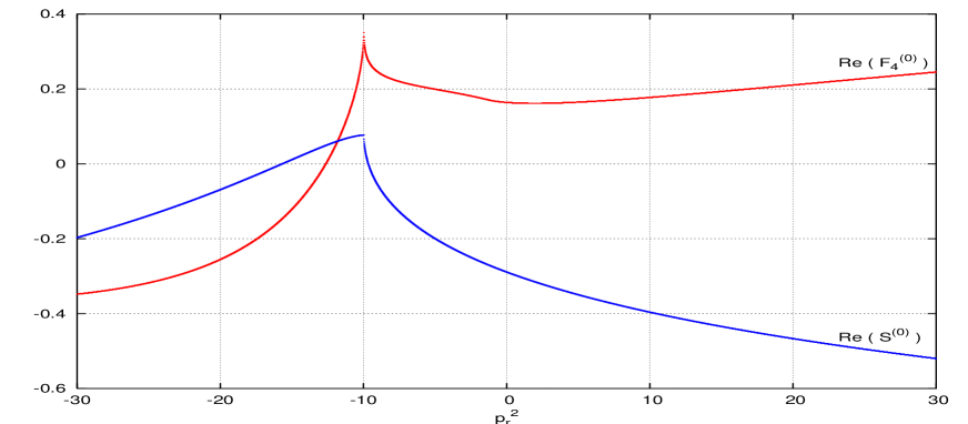
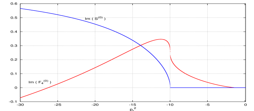
To illustrate some results of the program, and in the same time to show the behaviour of the function $F_{4}$ over a wide range of the variable $p_{r}^{2}$, we present here plots for two different sets of masses. In Fig. 2 we plot the values of $\hbox{Re~{}}F^{(0)}_{4}$ and $\hbox{Re~{}}S^{(0)}$ as functions of $p_{r}^{2}$, for the choice of the mass-values $m_{1}=2$, $m_{2}=1$, $m_{3}=4$, $m_{4}=20.1$ (arbitrary units). The 2-body threshold, $p^{2}=-(m_{1}+m_{4})^{2})\ ,$ corresponds to $p_{2b,th,r}^{2}=-9.96755102$. The presence of the 3-body threshold ($p_{3b,th,r}^{2}=-1,\$ due to the very definition of the scale $\mu$) is hardly visible from the $\hbox{Re~{}}F^{(0)}_{4}$ plot, but clearly from its imaginary part plotted in Fig.3. Its behaviour around the 2-body threshold is more ‘fuzzy’ due to the presence of root terms in the threshold expansion (see next section for an explicit form of the threshold expansion). The strikingly different behaviour of $F_{4}^{(0)}$ and $S^{(0)}$ near the 2-body threshold is due to additional logarithmic terms in the expansion of $F_{4}^{(0)}$, which are absent in $S^{(0)}$ expansion.

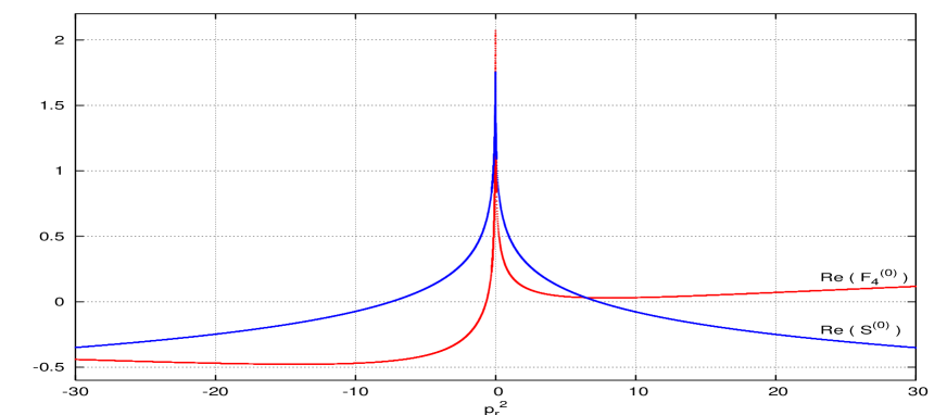
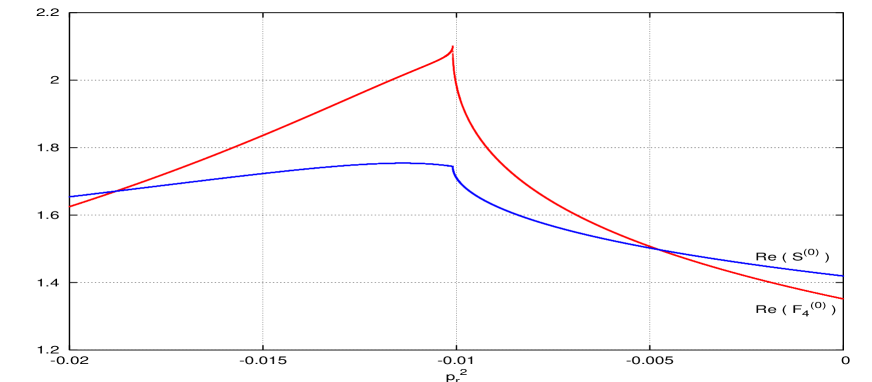
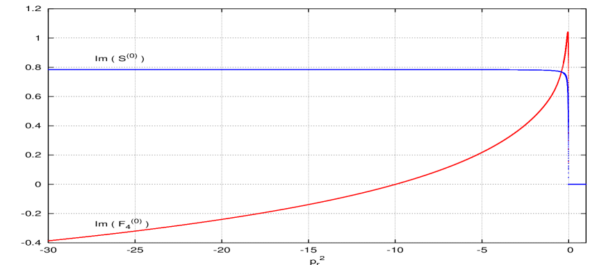
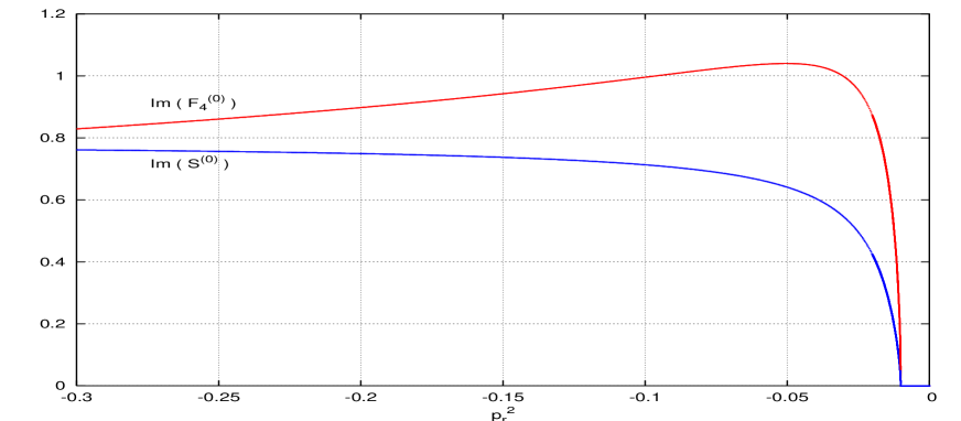
In Fig. 4 are plotted the values of $\hbox{Re~{}}F^{(0)}_{4}$ and $\hbox{Re~{}}S^{(0)}$ as a function of $p_{r}^{2}$, for the second choice of the mass-values, where one of the masses is considerably bigger than the others $m_{1}=1$, $m_{2}=9$, $m_{3}=200$, $m_{4}=20.1$. This time the higher threshold is the 2-body threshold at $p_{2b,th,r}^{2}=-0.010095465$, while the 3-body threshold is as always at $p_{3b,th,r}^{2}=-1$. Both functions show pronounced peaks around the 2-body threshold, and the ’zoom’ of the peaks in Fig. 5 shows that the qualitative behaviour of both functions nearby the 2-body threshold does not depend on masses (compare Fig. 2).

The imaginary part of $\hbox{Im~{}}F^{(0)}_{4}$ starts to be non vanishing at the 2-body threshold, as shown in Fig. 6, but this time no visible modification comes in at the 3-body threshold. The peaking behaviour of the imaginary parts is shown enlarged in Fig. 7.

In Table 1 are reported the benchmark values of $\hbox{Re~{}}F^{(0)}_{4}(m_{1}^{2},m_{2}^{2},m_{3}^{2},m_{4}^{2},p_{r}^{2})$ and $\hbox{Im~{}}F^{(0)}_{4}(m_{1}^{2},m_{2}^{2},m_{3}^{2},m_{4}^{2},p_{r}^{2})$ for the masses $m_{1}=1$, $m_{2}=9$, $m_{3}=200$, $m_{4}=20.1$, $\mu=m_{1}+m_{2}+m_{3}$.

The values at thresholds and pseudo-thresholds are obtained with the method discussed in the next section, the value at $p_{r}^{2}=0$ is from the analytic formula.

	$p^{2}_{r}$	$\hbox{Re~{}}F^{(0)}_{4}$	$\hbox{Im~{}}F^{(0)}_{4}$
	-30.	-0.44092793813(5)	-0.38633149701(4)
	-15.	-0.47753230147(5)	-0.13848347339(5)
	-1.5	-0.19215624308(2)	0.5235669521(1)
$p_{3b,th,r}^{2}$ =	-1.0	-0.0990578391(1)	0.60473101562(7)
	-0.99	-0.09669632676(2)	0.6066658942(1)
$p_{3b,ps3,r}^{2}$=	-0.981043	-0.094558472357(8)	0.60841511708(6)
	-0.9	-0.07412586818(2)	0.6249850792(1)
$p_{3b,ps2,r}^{2}$=	-0.835918	-0.056354400576(6)	0.63914196276(5)
	-0.825	-0.05316178728(1)	0.6416578704(1)
$p_{3b,ps1,r}^{2}$=	-0.818594	-0.051264529466(5)	0.64314892655(5)
	-0.8	-0.04565273027(1)	0.6475413524(1)
	-0.1	0.65325134562(1)	0.99590695379(1)
$p_{2b,th,r}^{2}$ =	-0.010095	2.101104208(4)	0.0
$p_{2b,ps,r}^{2}$ =	-0.008272	1.697672304903(6)	0.0
	0.0	1.351553692518424	0.0
	1.0	0.21346230166(6)	0.0
	30.0	0.117099162908(6)	0.0

Table 1: The benchmark values of $\hbox{Re~{}}F^{(0)}_{4}(m_{1}^{2},m_{2}^{2},m_{3}^{2},m_{4}^{2},p_{r}^{2})$ and $\hbox{Im~{}}F^{(0)}_{4}(m_{1}^{2},m_{2}^{2},m_{3}^{2},m_{4}^{2},p_{r}^{2})$ for the masses $m_{1}=1$, $m_{2}=9$, $m_{3}=200$, $m_{4}=20.1$, $\mu=m_{1}+m_{2}+m_{3}$.

5 Thresholds and pseudo-thresholds.

The numerical calculation with the system of MDE does not allow for $p_{r}^{2}$ much closer than $10^{-4}$ to the thresholds and pseudo-thresholds (special points), due to the numerical instability of the equations in these surrounding-domains. So a special treatment is required to get precise values of the MI’s there.

For the sunrise MI’s the analytical expansions at pseudo-thresholds [23] and at threshold [24] were previously obtained. In [18] these results were used as starting points for the system of MDE’s for the sunrise MI’s to get reliable results in the surrounding-domain of these points. However this method is not universal, as it requires a separate analytic calculation of the MI expansion at these points, which is difficult and probably not always possible.

We discuss here in detail the features, advantages and limitations of an approximation method, which is rather precise, universal and easy to use. This method was recently proposed in [20]. However the ’universal’ approximant suggested by the author applies only to some cases and fails at the 2-body threshold relevant for the present calculations.

The method consists in the construction of a suitable approximant of the MI, which due to the smallness of the surrounding-domain is naturally the expansion of the MI around the considered special point. The proper form of the expansion (with undetermined coefficients) around each special point can easily be deduced from the MDE’s themselves [25].

The coefficients of the approximant are calculated using numerical values of the MI, obtained solving the system of MDE for some points nearby the special point, but outside its surrounding-domain to avoid numerical instability. The approximant is used to get the values of the MI at the special point and within its surrounding-domain. Note that the proper form of the expansion around a special point is crucial to produce right results around special points. With the wrong choice of the approximant one may still get the values at the special points right, when the points chosen for the approximant ‘construction’ are symmetrically distributed around the special point. The values obtained for the surrounding-domains will be however wrong.

To test the precision of this approximation method, we compare its result at the special point with that obtained from analytic result there, when available, and in the surrounding-domain with the result given by the advanced numerical solution of the MDE’s started from the special point. Of course the approximation method can be used also in a region where a MI does not contain a special point to test the precision of the method.

The 2 and 3-body pseudo-thresholds are the simplest points to be treated in this way: as they are regular points the approximant can simply be the power expansion. For each MI ($F_{i}^{(0)},\ i=0,1,2,3,4$ and $S^{(0)}$) in each of its pseudo-thresholds can be used an approximant of the type

$$F(x)=a_{0}+a_{1}x+a_{2}x^{2}+a_{3}x^{3}\ ,$$ (23)

where $x=p_{r}^{2}-p_{ps,r}^{2}$ and $p_{ps,r}^{2}$ is the value of $p_{r}^{2}$ at the pseudo-threshold. As we want to use $x$ well below $10^{-4}$, in Eq.(23) it is enough to use four terms in the expansion, the truncation causing a relative error of the order of $x^{4}=10^{-16}$. The actual implementation of $F(x)$ uses the four points $x=\pm 10^{-4},\pm 0.5\cdot 10^{-4}$ to calculate the four coefficients $a_{i},\ \ i=0,1,2,3$, the error associated to its value is dominated by the error coming from the numerical calculation of the MI at these points. It has to be noted that the coefficients of the expansion Eq.(23) can be complex if the expanded function is complex valued – as it is the case above threshold(s).

The values of the sunrise MI’s $\ F_{i}^{(0)},\ i=0,1,2,3$ at the 3-body pseudo-thresholds and of the 1-loop self-mass MI $\ S^{(0)}$ at the 2-body pseudo-threshold, can be obtained from known analytical formulas [23, 17]. The approximation method can reach in the implemented program a relative error of the order of $10^{-11}-10^{-12}$ and its results are always in agreement with the analytical ones within this error.

In the surrounding-domain (where $x<0.5\cdot 10^{-4}$) of the 3-body pseudo-threshold approximation method results for the sunrise MI’s are in agreement with the results obtained from MDE advancing solution starting from the pseudo-threshold [18] within a relative accuracy of the order of $10^{-9}$, which is the best accuracy obtainable by the MDE advancing solution program in this region. However, as the approximation method values for $F_{i}^{(0)},\ i=0,1,2,3$, and $S^{(0)}$ reproduce well the values from analytical formulas at the pseudo-thresholds, and from MDE advancing solution program starting from $p_{r}^{2}=0$ in all tested points outside the surrounding-domain (where $x\geq 0.5\cdot 10^{-4}$), we are confident that the approximation method is better and that the stated relative accuracy of order $10^{-11}-10^{-12}$ is a safe estimate.

At the 3-body threshold the proper approximants for the $F_{i}^{(0)},\ i=0,1,2,3,4\$ are

$$F_{i}^{(0)}(x)=a_{i,0}+\left(a_{i,1}+b_{i,1}\log(x)\right)x+\left(a_{i,2}+b_{i,2}\log(x)\right)x^{2}+\left(a_{i,3}+b_{i,3}\log(x)\right)x^{3}\ ,$$ (24)

where $x=p_{r}^{2}-p_{3b,th,r}^{2}$ and $p_{3b,th,r}^{2}=-(m_{1,r}+m_{2,r}+m_{3,r})^{2}=-1$. We use $x=\pm 0.5\cdot 10^{-4},\pm 10^{-4},\pm 1.5\cdot 10^{-4},\pm 2\cdot 10^{-4}$ to obtain numerically the coefficients $a_{i,j},\ i=0,1,2,3,4,\ j=0,1,2,3$ and $b_{i,k},\ k=1,2,3$. Again all the coefficients in the expansion of $F_{4}^{(0)}$ can be complex depending on the values of the 2-body and 3-body thresholds. For $S^{(0)}$ we use Eq.(23) as it is regular at the 3-body threshold.

Comparisons with the analytical results for the sunrise MI at the 3-body threshold [18] and other tests like those at pseudo-thresholds were performed with the same conclusions, so again a precision of the order of $10^{-11}-10^{-12}$ can be assumed.

At the 2-body threshold the proper approximants for $S^{(0)}$ and $F_{4}^{(0)}$ are

$$\kern-10.0ptS^{(0)}=a_{S,0}+a_{S,1}x+a_{S,2}x^{2}+a_{S,3}x^{3}+\sqrt{x}\ \left(b_{S,0}+b_{S,1}x+b_{S,2}x^{2}+b_{S,3}x^{3}\right)\ ,$$

$$\kern-10.0ptF_{4}^{(0)}=a_{4,0}+a_{4,1}x+a_{4,2}x^{2}+a_{4,3}x^{3}+\sqrt{x}\ \biggl{[}b_{4,0}+b_{4,1}x+b_{4,2}x^{2}+b_{4,3}x^{3}\biggr{]}$$

$$\kern 14.0pt+\sqrt{x}\log(x)\biggl{[}c_{4,0}+c_{4,1}x+c_{4,2}x^{2}+c_{4,3}x^{3}\biggr{]}$$ (25)

where $x=p_{r}^{2}-p_{2b,th,r}^{2}$ and $p_{2b,th,r}^{2}=-(m_{1,r}+m_{4,r})^{2}$. The threshold expansion can be easily derived from Eq.(12) for $F_{4}^{(0)}$, while for $S^{(0)}$ it was given in [17]. The real constants $a_{S,j},\ b_{S,j}$ and real or complex constants $a_{4,j},\ b_{4,j},c_{4,j},\ j=0,1,2,3$ (see discussion above) are obtained calculating numerically with the MDE advancing solution the values of $S^{(0)}$ at $x=\pm i\cdot 10^{-3}$, $x=\pm i\cdot 0.5\cdot 10^{-3}$, $x=\pm i\cdot 0.25\cdot 10^{-3}$, $x=\pm i\cdot 0.125\cdot 10^{-3}$, and of $F_{4}^{(0)}$ there and also at $x=\pm i\cdot 0.0625\cdot 10^{-3}$, $x=\pm i\cdot 0.03125\cdot 10^{-3}$. The choice of imaginary values for $x$ allows to overcome the numerical problems arising in the present case for real values of $x$ when $|x|<10^{-4}$ with the usual MDE advancing solution program starting from $p_{r}^{2}=0$, due to the steep behaviour of the functions $S^{(0)}$ and $F_{4}^{(0)}$ nearby the 2-body threshold, as can be seen in Fig. 5. On the other hand the MI values at $|x|<10^{-4}$ are needed to get enough precise values for the coefficients in the approximants. For $F_{i}^{(0)},\ (i=0,1,2,3)$ we use Eq.(23) as approximants.

For the $S^{(0)}$ approximant values a relative precision of the order of $10^{-11}-10^{-12}$ is obtained as before, confirmed by the comparisons with the analytic result.

For the $F_{4}^{(0)}$ approximant values the contrasting requirements does not allow a relative precision better than $10^{-8}-10^{-9}$.

6 Comparisons.

Numerical values for the MI of Eq.(1) for non-vanishing values of the masses are reported in literature, only for small values of time-like $p^{2}$, in [7] and more extensively in [8]. More precisely there was calculated the quantity

$$T_{1234N}(\bar{p}^{2};\bar{m}_{1}^{2},\bar{m}_{2}^{2},\bar{m}_{3}^{2},\bar{m}_{4}^{2})\equiv T_{1234}(\bar{p}^{2};\bar{m}_{1}^{2},\bar{m}_{2}^{2},\bar{m}_{3}^{2},\bar{m}_{4}^{2},\mu^{2})-T_{1234}(\bar{p}^{2};\bar{m}_{1}^{2},\bar{m}_{2}^{2},0,0,\mu^{2})$$

$$=16F_{4}^{(0)}(m_{1}^{2},m_{2}^{2},m_{3}^{2},m_{4}^{2},p^{2},\mu^{2})-T_{1234}^{(0)}(-p^{2};m_{4}^{2},m_{1}^{2},0,0,\mu^{2})+\frac{1}{2}\zeta(2)\ ,$$ (26)

with $T-$functions defined in [7, 8]. The function $T_{1234N}(\bar{p}^{2};\bar{m}_{1}^{2},\bar{m}_{2}^{2},\bar{m}_{3}^{2},\bar{m}_{4}^{2})$ is finite in the $n\to 4$ limit and it is independent from $\mu^{2}$, the arbitrary mass scale introduced in Eq.(1). Here the $\mu^{2}$ dependence is explicitly shown, whenever present. The quantity $T_{1234}(\bar{p}^{2};\bar{m}_{1}^{2},\bar{m}_{2}^{2},\bar{m}_{3}^{2},\bar{m}_{4}^{2},\mu^{2})$ is like the MI of Eq.(1), with a different normalization factor, which results in the factor $16$ and the additive quantity $\zeta(2)/2$, the second line of Eq.(26). The analytical expression for $T_{1234}(\bar{p}^{2};\bar{m}_{1}^{2},\bar{m}_{2}^{2},0,0,\mu^{2})$ is given in [26].

Due to the different assignment of the mass indexes ($m_{i}$) to the lines in our Fig.1 with respect to the correspondent ones ($\bar{m}_{j}$) in [7, 8, 26], we have the correspondence $m_{1}=\bar{m}_{2}=3$, $m_{2}=\bar{m}_{4}=7$, $m_{3}=\bar{m}_{3}=5$, $m_{4}=\bar{m}_{1}=1$, where the numerical values are for the comparison with Table 1 of [8]. One has also $\bar{p}^{2}=-p^{2}$, due to Minkowski-Euclidean space transformation. In the second line of Eq.(26) $F_{4}^{(0)}(m_{1}^{2},m_{2}^{2},m_{3}^{2},m_{4}^{2},p^{2},\mu^{2})$ is calculated through the differential equation Eq.(12) and $T_{1234}^{(0)}(-p^{2};m_{4}^{2},m_{1}^{2},0,0,\mu^{2})$ is the finite part in the $n\to 4$ limit of $T_{1234}(-p^{2};m_{4}^{2},m_{1}^{2},0,0,\mu^{2})$ from [26].

$p^{2}$	A	B
-2.66667	-8.45038098750(31)	-8.45038
-1.77778	-8.28747181582(32)	-8.28747
-1.18519	-8.18480592994(33)	-8.18481
-0.790124	-8.11877664655(31)	-8.11878
-0.526749	-8.07577187774(28)	-8.07577
-0.351166	-8.04753658726(33)	-8.04754
-0.234111	-8.02890161217(30)	-8.02890
-0.156074	-8.01656069505(26)	-8.01656
-0.104049	-8.00836962582(21)	-8.00837
-0.069366	-8.00292496915(41)	-8.00292
-0.046244	-7.99930227781(36)	-7.99930
-0.030829	-7.99689023488(21)	-7.99689
-0.020553	-7.99528370180(10)	-7.99528
-0.013702	-7.99421324511(10)	-7.99421
-0.009135	-7.99349993358(10)	-7.99350
-0.006090	-7.99302446227(10)	-7.99302

Table 2: Values of $T_{1234N}(\bar{p}^{2};\bar{m}_{1}^{2},\bar{m}_{2}^{2},\bar{m}_{3}^{2},\bar{m}_{4}^{2})$ for small values of $\bar{p}^{2}=-p^{2}$. The masses are $m_{1}=\bar{m}_{2}=3$, $m_{2}=\bar{m}_{4}=7$, $m_{3}=\bar{m}_{3}=5$, $m_{4}=\bar{m}_{1}=1$. In column A are reported the results of the present method, with in brackets the error in the last digits, in column B are reported the results from column D of Table 1 of [8], to whom barred notation refers.

Our results are shown in column A of Table 2 and are in complete agreement with the results in column D of Table 1 of [8], obtained from a one-dimensional integral representation and reported also here in column B for the reader’s convenience. The results are purely real for small values of $|p^{2}|$, i.e. smaller than the smallest threshold value, which for the chosen values of the masses is the 3-body threshold of $T_{1234}^{(0)}(-p^{2};m_{4}^{2},m_{1}^{2},0,0,\mu^{2})$, corresponding to $p^{2}=-(m_{1}+0+0)^{2}=-9$.

Recently in [20] a calculation with the same method has provided the MDE and the expansion at $p^{2}=0$ for all the 2-loop self-mass MI. Some numerical results are presented there for the function $U$ corresponding to $F_{4}^{(0)}$, that we have verified up to the 9 digits reported in [20]. The comparison is by no means simple, due to the different definition of the pole-term in the 4-denominator function in [20]. The finite terms of $U$ and $F_{4}$ differ and the term proportional to $(n-4)$ of the Laurent-expansion of the 1-loop self-mass MI, that we take from [27], is necessary to account for that difference.

7 Conclusions.

We presented the results of the analytical expansion around $p^{2}=0$ and of the numerical calculation of the MI related to the general massive 2-loop 4-denominator self-mass diagram, using the 4-th order Runge-Kutta advancing solution method applied to the MDE satisfied by the MI.

An approximation method, suggested in [20], was properly developed here, allowing for precise numerical evaluation of the MI’s even in the surrounding-domains of the special points.

The relative precision reached by the developed numerical program is of the order of 10^-11–10^-12 for all points, but the surrounding-domain of the 2-body threshold, where the relative precision is ‘only’ of the order of 10^-8–10^-9.

It is to be emphasized that the method requires only the knowledge of Master Differential Equations (MDE’s) satisfied by the MI’s. The initial conditions follow from requirement of the regularity of MI at $p^{2}=0$ and MDE, while the form of the approximants used in the surrounding-domains of the special points follows from the MDE only.

Acknowledgments. Henryk Czyż and Agnieszka Grzelińska are grateful to the Bologna Section of INFN and to the Department of Physics of the Bologna University for support and kind hospitality.

Figure 2: Plots of $\hbox{Re~{}}F^{(0)}_{4}(m_{1}^{2},m_{2}^{2},m_{3}^{2},m_{4}^{2},p_{r}^{2})$ and $\hbox{Re~{}}S^{(0)}(m_{1}^{2},m_{4}^{2},p_{r}^{2})$ as a function of $p_{r}^{2}$ for $m_{1}=2$, $m_{2}=1$, $m_{3}=4$, $m_{4}=20.1$ and $\mu=m_{1}+m_{2}+m_{3}$.

Figure 3: Plots of $\hbox{Im~{}}F^{(0)}_{4}(m_{1}^{2},m_{2}^{2},m_{3}^{2},m_{4}^{2},p_{r}^{2})$ and $\hbox{Im~{}}S^{(0)}(m_{1}^{2},m_{4}^{2},p_{r}^{2})$ as a function of $p_{r}^{2}$ for $m_{1}=2$, $m_{2}=1$, $m_{3}=4$, $m_{4}=20.1$ and $\mu=m_{1}+m_{2}+m_{3}$.

Figure 4: Plots of $\hbox{Re~{}}F^{(0)}_{4}(m_{1}^{2},m_{2}^{2},m_{3}^{2},m_{4}^{2},p_{r}^{2})$ and $\hbox{Re~{}}S^{(0)}(m_{1}^{2},m_{4}^{2},p_{r}^{2})$ as a function of $p_{r}^{2}$ for $m_{1}=1$, $m_{2}=9$, $m_{3}=200$, $m_{4}=20.1$ and $\mu=m_{1}+m_{2}+m_{3}$.

Figure 5: Enlargements for the peaks of the plots of $\hbox{Re~{}}F^{(0)}_{4}(m_{1}^{2},m_{2}^{2},m_{3}^{2},m_{4}^{2},p_{r}^{2})$ and $\hbox{Re~{}}S^{(0)}(m_{1}^{2},m_{4}^{2},p_{r}^{2})$ as a function of $p_{r}^{2}$ for $m_{1}=1$, $m_{2}=9$, $m_{3}=200$, $m_{4}=20.1$ and $\mu=m_{1}+m_{2}+m_{3}$.

Figure 6: Plots of $\hbox{Im~{}}F^{(0)}_{4}(m_{1}^{2},m_{2}^{2},m_{3}^{2},m_{4}^{2},p_{r}^{2})$ and $\hbox{Im~{}}S^{(0)}(m_{1}^{2},m_{4}^{2},p_{r}^{2})$ as a function of $p_{r}^{2}$ for $m_{1}=1$, $m_{2}=9$, $m_{3}=200$, $m_{4}=20.1$ and $\mu=m_{1}+m_{2}+m_{3}$.

Figure 7: Enlargements for the peaks of the plots of $\hbox{Im~{}}F^{(0)}_{4}(m_{1}^{2},m_{2}^{2},m_{3}^{2},m_{4}^{2},p_{r}^{2})$ and $\hbox{Im~{}}S^{(0)}(m_{1}^{2},m_{4}^{2},p_{r}^{2})$ as a function of $p_{r}^{2}$ for $m_{1}=1$, $m_{2}=9$, $m_{3}=200$, $m_{4}=20.1$ and $\mu=m_{1}+m_{2}+m_{3}$.

References

- [1] F.V. Tkachov, Phys. Lett.B 100, 65 (1981); K.G. Chetyrkin and F.V. Tkachov, Nucl. Phys.B 192, 159 (1981).
- [2] O.V. Tarasov, Nucl. Phys.B 502, 455 (1997), hep-ph/9703319.
- [3] R. Mertig and R. Scharf, Comput. Phys. Commun.111, 265 (1998), hep-ph/9801383.
- [4] M. Caffo, H. Czyż, S. Laporta and E. Remiddi, Nuovo Cim.A 111, 365 (1998), hep-th/9805118.
- [5] M. Caffo, H. Czyż, S. Laporta and E. Remiddi, Acta Phys. Pol.B 29, 2627 (1998), hep-th/9807119.
- [6] F.A. Berends, M. Böhm, M. Buza and R. Scharf, Z. Phys.C 63, 227 (1994).
- [7] F.A. Berends and J.B. Tausk, Nucl. Phys.B 421, 456 (1994).
- [8] S. Bauberger, F.A. Berends, M. Böhm and M. Buza, Nucl. Phys.B 434, 383 (1995), hep-ph/9409388.
- [9] A. Ghinculov and J.J. van der Bij, Nucl. Phys.B 436, 30 (1995), hep-ph/9405418.
- [10] P. Post and J.B. Tausk, Mod. Phys. Lett.A 11, 2115 (1996), hep-ph/9604270.
- [11] S. Groote, J.G. Körner and A.A. Pivovarov, Eur. Phys. J.C 11, 279 (1999), hep-ph/9903412; Nucl. Phys.B 542, 515 (1999), hep-ph/9806402.
- [12] G. Amorós, J. Bijnens and P. Talavera, Nucl. Phys.B 568, 319 (2000), hep-ph/9907264.
- [13] G. Passarino, Nucl. Phys.B 619, 257 (2001), hep-ph/0108252.
- [14] G. Passarino and S. Uccirati, Nucl. Phys.B 629, 97 (2002), hep-ph/0112004.
- [15] S. Laporta, Int. J. Mod. Phys.A 15, 5087 (2000), hep-ph/0102033; Phys. Lett.B 504, 188 (2001), hep-ph/0102032.
- [16] A.V. Kotikov, Phys. Lett.B254, 158 (1991), hep-ph/9807440 (1998).
- [17] E. Remiddi, Nuovo Cim.A110, 1435 (1997), hep-th/9711188 (1997).
- [18] M. Caffo, H. Czyż and E. Remiddi, Nucl. Phys.B 634, 309 (2002), hep-ph/0203256.
- [19] W.H. Press, S.A. Teukolsky, W.T. Vetterling, B.P. Flannery Numerical Recipes in FORTRAN. The Art of Scientific Computing., Cambridge University Press, 1994.
- [20] S.P. Martin, Phys. Rev.D 68, 075002 (2003), hep-ph/0307101.
- [21] C. Ford, I. Jack and D.R.T. Jones, Nuc. Phys. B 387, 373 (1992)
- [22] A.I. Davydychev and J.B. Tausk, Nuc. Phys. B 397, 123 (1993); A.I. Davydychev, V.A. Smirnov and J.B. Tausk, Nuc. Phys. B 410, 325 (1993), hep-ph/9307371
- [23] M. Caffo, H. Czyż and E. Remiddi, Nucl. Phys.B 581, 274, (2000), hep-ph/9912501, see also the Appendix of [18].
- [24] M. Caffo, H. Czyż and E. Remiddi, Nucl. Phys.B 611, 503, (2001), hep-ph/0103014, see also the Appendix of [18].
- [25] E.L. Ince, Ordinary differential equations, Dover Publications, New York, 1956.
- [26] R. Scharf and J.B. Tausk, Nucl. Phys.B 412, 523 (1994).
- [27] F. Jegerlehner, M. Yu. Kalmykov and O. Veretin, Nucl. Phys.B 641, 285 (2002), hep-ph/0105304.