BU-HEPP-03-11,UTHEP-03-1101
Nov, 2003

Massive Elementary Particles and Black Holes^†

B.F.L. Ward
Department of Physics,
Baylor University, Waco, Texas 76798-7316, USA
and
Department of Physics and Astronomy,
The University of Tennessee, Knoxville, Tennessee 37996-1200, USA

Abstract

An outstanding problem posed by Einstein’s general theory of relativity to the quantum theory of point particle fields is the fate of a massive point particle; for, in the classical solutions of Einstein’s theory, such a system should be a black hole. We use exact results in a new approach to quantum gravity to show that this conclusion is obviated by quantum loop effects. Phenomenological implications are discussed.

Submitted to JCAP

• Work partly supported by the US Department of Energy Contract DE-FG05-91ER40627 and by NATO Grant PST.CLG.977751.

The ideas of Albert Einstein in the special theory of relativity have been incorporated into quantum mechanics so that we can say the union of Niels Bohr and Albert Einstein has been achieved in the theory of special relativistic point particle quantum fields. Indeed, the proto-typical example of such a theory is the Standard Model ( SM ) [1, 2] and its successes are a true triumph of the 20th century. However, for Einstein’s theory of general relativity, the situation regarding its union with quantum mechanics is markedly different; for, even though his general theory of relativity has had also many successes [3, 4], it has so far evaded a complete, direct application of quantum mechanics. All of the accepted treatments of the complete quantum loop corrections to Einstein’s theory involve recourse to as yet phenomenologically unfounded theoretical paradigms [5, 6] which seem to imply even the modification of quantum mechanics itself. In Ref. [7], we have introduced a new approach to quantum gravity wherein we use resummation of large higher order radiative corrections to ameliorate the apparently bad UV behavior of the theory. This new approach, which relies on phenomenologically well-founded theoretical paradigms and which does not involve any modification of quantum mechanics itself, allows us to analyze truly complete finite quantum loop effects in Einstein’s general theory of relativity. In this paper, we present such an analysis.

It is important to put our approach in the proper context of the current literature on quantum general relativity, which is an extensive literature indeed [8]. The situation was already summarized by Weinberg in Ref. [9]. There, Weinberg argued that there are basically four approaches to the bad UV behavior of quantum general relativity:

• extended theories of gravitation: supersymmetric theories - superstrings

• resummation

• composite gravitons

• asymptotic safety: fixed point theory ( see Ref. [10] )

In what follows, we discuss a new version of the resummation approach based on the methods of Yennie, Frautschi and Suura (YFS) in Ref. [11]. Since these methods are not generally familiar, we review their essence as well in what follows.

The key element in the YFS approach to resummation is the rearrangement of the respective series in such away that the large real and virtual corrections from the infrared regime are summed up to all orders. In Abelian gauge theories, the resummation results in exponential factors which contain all of the IR singularities and these exactly cancel between real and virtual corrections in the exponential factors for physical observables. In non-Abelian gauge theories, not all IR singularities exponentiate in the YFS expansion so that, after the YFS rearrangement, the respective residuals still exhibit a final cancellation [12] between real and virtual corrections in the physical observables order by order in the loop expansion. In the quantum theory of general relativity, wherein the symmetry group is non-Abelian, application of the YFS methods then allows us to isolate the large IR contributions to the loop expansion which do exponentiate and resum them in an exact rearrangement of the respective loop expansion [7]. The remarkable result is that, having done this, the remaining expansion becomes much more convergent in the ultra-violet (UV) regime than was the original expansion. Indeed, the UV infinities are completely removed by the YFS resummation. It is this result that we will apply in the discussion which follows.

It may seem somewhat paradoxical that the infrared regime of a theory could produce, upon resummation, an exact rearrangement of the respective perturbation series in which the ultra-violet regime of the resummed series is much better behaved than the original series. What one needs to recall here is that, in the loop expansion, the integration over the 4-dimensional loop momentum, $\int d^{4}k$, generates enhanced contributions in point particle quantum field theory in three regimes:

• the infrared regime (IR)

• the collinear regime (CL)

• the ultra-violet regime (UV).

The usual renormalization program subtracts the UV divergent parts of the integration and thereby renders the integral convergent in the UV regime were it not already so. The remaining large contributions from the IR and CL regimes then also make an enhanced contribution to the result of the integration whenever they are divergent or posses would-be mass singularities that would render them divergent when a mass goes to zero. The latter result in big logs, $L\equiv\ln Q^{2}/m^{2}$, $\ell\equiv\ln Q^{2}/\lambda^{2}$, appearing to an attendant power as a result of the integration, where we treat $Q$ as a generic hard scale in the problem, m a typical external light particle mass, and $\lambda$ as an infrared regulator mass for massless non-zero integer spinning particles. These big logs are just as large in general as any big logs left-over from the UV subtraction in the renormalization program and hence are just as important, if not more important, than the latter. It is the YFS rearrangement of these important IR terms in the virtual corrections that the new approach to quantum gravity in Ref. [7] uses to tame the UV behavior of quantum general relativity. It follows that, as the graviton couples to all point particles, this type of improvement of the UV behavior found in Ref. [7] applies to all renormalizable point particle quantum field theories and to a large class of non-renormalizable point particle quantum field theories that includes quantum general relativity, of course.

Here, we need to stress that, while we are making a YFS resummation of the theory of quantum general relativity, we are in fact focusing on the UV regime of the theory, the regime of sub-Planck length physics. This should be compared with the rather complementary efforts in Refs.  [13], which use the analog of the chiral perturbation theory familiar from the strong interaction and address then large distance limit of quantum general relativity. We see no contradiction between the new resummed approach in Ref. [7] and the large distance, effective Lagrangian methods of Refs. [13]. The relationship between the two is the same as the relationship between the use of perturbative QCD ( Quantum Chromodynamics [2] ) for the hard strong interactions and the use of chiral perturbation theory for the soft, large distance strong interactions, where there should be then a matching between the respective large distance and short distance formalisms at some appropriate intermediate scale – sometimes in QCD this has to be done using fully non-perturbative methods and we see no reason why the similar situation might not hold in the quantum theory of general relativity. We hope to come back to these types of analyses elsewhere [14].

Currently, the only really accepted approach to quantum general relativity is that embodied in the well-known but incompletely understood superstring theory [5, 6]. Therefore, one of the main results of the resummed quantum gravity theory of Ref. [7], using the superstring as a benchmark, is to provide an alternative view of the important problem of quantum general relativity. There is one fundamental difference between the two approaches: in the superstring theory, the Planck length is special, and one really can not readily consider physics below it whereas in the new, resummed quantum gravity there is no problem at all to discuss sub-Planck scale physics. The situation reminds one of the old string theory [15] approach to the strong interaction in the 1960’s and early 1970’s, wherein the size of a hadron, $\sim 1$fm, was special and it was difficult to discuss sub-fermi physics. We of course have since learned that the old string theory of the strong interaction was just a phenomenological model for the point particle field theory of QCD, the truly fundamental description of the strong interaction. Evidently, our new, resummed quantum gravity theory suggests that the same story may occur again – namely, the extended object theory, the superstring in this case, is really just a phenomenological model for a more fundamental point particle quantum field theory that describes quantum general relativity to sub-Planck scale distances as well. Presumably, the superstring theory can help us determine just what this truly fundamental theory, which would describe all the known forces to arbitrary distances below the Planck scale, would be. Here, we refer to it as TUT, the ultimate theory. We hope to participate in its construction elsewhere [14].

At this point, the reader may be wondering how, if ever, observations could probe the sub-Planck scale regime? We do know that quantum loop corrections do probe arbitrary scales so that sufficiently precise measurements of appropriately chosen quantities must be sensitive to sub-Planck scale physics. It is also natural to speculate that the the early universe may provide such observables? Here, however, there is controversy. In Ref. [16], it is stated that there are about 8 orders of magnitude between what scale astrophysical observations can easily probe today and the Planck scale. This is not an insurmountable difference in scales, as either appropriate observables and/or appropriate precision can easily overcome as many as 16 orders of magnitude, as in proton decay studies [17]. We do, however, need to find other arenas in which to try to develop tests of the physics in the sub-Planck scale regime governed by TUT. We return to this discussion elsewhere.

There will be some immediate results that the new resummed theory can provide that amount to cross checks on it that are outside of the regime of applicability of the superstring, for example. In the new approach, a point particle is something fundamental, in the superstring, a point particle is a large distance approximation. Therefore, in the new theory there will be questions to answer that do not occur in the superstring. One of these concerns the issue of the black hole character of a massive point particle in the classical theory of general relativity. For, in Einstein’s theory, a point particle of non-zero rest mass $m$ has a non-zero Schwarzschild radius $r_{S}=2(m/M_{Pl})(1/M_{Pl})$, where $M_{Pl}$, $1.22\times 10^{19}$ GeV, is the Planck mass, so that such a particle should be a black hole [3] in the classical solutions of Einstein’s theory, unable to communicate “freely” with the world outside of its Schwarzschild radius, except for some thermal effects first pointed-out by Hawking [18]. Surely, this poses a problem for the Standard Model phenomenology: it seems these point particles are communicating freely their entire selves in their interactions with each other. Can our new quantum theory of gravity reconcile this apparent contradiction? It this question that we address here.

We start our analysis by setting up our new approach to quantum gravity. As we explain in Ref. [7], we follow the idea of Feynman [19, 20] and treat Einstein’s theory as a point particle field theory in which the metric of space-time undergoes quantum fluctuations just like any other point particle does. On this view, the Lagrangian density of the observable world is

$${\cal L}(x)=-\frac{1}{2\kappa^{2}}\sqrt{-g}R+\sqrt{-g}L^{\cal G}_{SM}(x)$$ (1)

where $R$ is the curvature scalar, $-g$ is the negative of the determinant of the metric of space-time $g_{\mu\nu}$, $\kappa=\sqrt{8\pi G_{N}}\equiv\sqrt{8\pi/M_{Pl}^{2}}$, where $G_{N}$ is Newton’s constant, and the SM Lagrangian density, which is well-known ( see for example, Ref. [1, 21] ) when invariance under local Poincare symmetry is not required, is here represented by $L^{\cal G}_{SM}(x)$ which is readily obtained from the familiar SM Lagrangian density as described in Ref. [22]. It is well-known that there are many massive point particles in (1). According to classical general relativity, they should all be black holes, as we noted above. Are they black holes in our new approach to quantum gravity? To study this question, we continue to follow Feynman in Ref. [19, 20] and treat spin as an inessential complication [23], as the question of whether a point particle with mass is or is not a black hole should not depend too severely on whether or not it is spinning. We can come back to a spin-dependent analysis elsewhere [14].

Thus, we replace $L^{\cal G}_{SM}(x)$ in (1) with the simplest case for our question, that of a free scalar field , a free physical Higgs field, $\varphi(x)$, with a rest mass believed [24] to be less than $400$ GeV and known to be greater than $114.4$ GeV with a 95% CL. We are then led to consider the representative model

$$\begin{split}{\cal L}(x)&=-\frac{1}{2\kappa^{2}}R\sqrt{-g}+\frac{1}{2}\left(g^{\mu\nu}\partial_{\mu}\varphi\partial_{\nu}\varphi-m_{o}^{2}\varphi^{2}\right)\sqrt{-g}\\ &=\quad\frac{1}{2}\left\{h^{\mu\nu,\lambda}\bar{h}_{\mu\nu,\lambda}-2\eta^{\mu\mu^{\prime}}\eta^{\lambda\lambda^{\prime}}\bar{h}_{\mu_{\lambda},\lambda^{\prime}}\eta^{\sigma\sigma^{\prime}}\bar{h}_{\mu^{\prime}\sigma,\sigma^{\prime}}\right\}\\ &\qquad+\frac{1}{2}\left\{\varphi_{,\mu}\varphi^{,\mu}-m_{o}^{2}\varphi^{2}\right\}-\kappa{h}^{\mu\nu}\left[\overline{\varphi_{,\mu}\varphi_{,\nu}}+\frac{1}{2}m_{o}^{2}\varphi^{2}\eta_{\mu\nu}\right]\\ &\quad-\kappa^{2}\left[\frac{1}{2}h_{\lambda\rho}\bar{h}^{\rho\lambda}\left(\varphi_{,\mu}\varphi^{,\mu}-m_{o}^{2}\varphi^{2}\right)-2\eta_{\rho\rho^{\prime}}h^{\mu\rho}\bar{h}^{\rho^{\prime}\nu}\varphi_{,\mu}\varphi_{,\nu}\right]+\cdots\\ \end{split}$$ (2)

Here, $\varphi(x)_{,\mu}\equiv\partial_{\mu}\varphi(x)$, and $g_{\mu\nu}(x)=\eta_{\mu\nu}+2\kappa h_{\mu\nu}(x)$ where we follow Feynman and expand about Minkowski space so that $\eta_{\mu\nu}=diag\{1,-1,-1,-1\}$. Following Feynman, we have introduced the notation $\bar{y}_{\mu\nu}\equiv\frac{1}{2}\left(y_{\mu\nu}+y_{\nu\mu}-\eta_{\mu\nu}{y_{\rho}}^{\rho}\right)$ for any tensor $y_{\mu\nu}$. Thus, $m_{o}$ is the bare mass of our free Higgs field and we set the small tentatively observed [25] value of the cosmological constant to zero so that our quantum graviton has zero rest mass. The Feynman rules for (2) have been essentially worked out by Feynman [19, 20], including the rule for the famous Feynman-Faddeev-Popov [19, 26] ghost contribution that must be added to it to achieve a unitary theory with the fixing of the gauge ( we use the gauge of Feynman in Ref. [19], $\partial^{\mu}\bar{h}_{\nu\mu}=0$ ), so we do not repeat this material here. We turn instead directly to the issue of the effect of quantum loop corrections on the black hole character of our massive Higgs field.

We initiate our approach by calculating the effects of the diagrams in Fig. 1 on the graviton propagator. These effects give the possible one-loop corrections to Newton’s law that would follow from the matter in (2) and will directly impact our black hole issue.

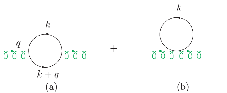
Figure 1: The scalar one-loop contribution to the graviton propagator. $q$ is the 4-momentum of the graviton.

In Ref. [7], we have shown that, while the naive power counting of the graphs gives their degree of divergence as +4, YFS [11] resummation of the soft graviton effects in the propagators in Fig. 1 renders the graphs ultra-violet (UV) finite. Indeed, for example, for Fig. 1a, we get without YFS resummation the result

$$i\Sigma(q)^{1a}_{\bar{\mu}\bar{\nu};\mu\nu}=\kappa^{2}\frac{\int d^{4}k}{2(2\pi)^{4}}\frac{\left(k^{\prime}_{\bar{\mu}}k_{\bar{\nu}}+k^{\prime}_{\bar{\nu}}k_{\bar{\mu}}\right)\left(k^{\prime}_{\mu}k_{\nu}+k^{\prime}_{\nu}k_{\mu}\right)}{\left({k^{\prime}}^{2}-m^{2}+i\epsilon\right)\left(k^{2}-m^{2}+i\epsilon\right)}$$ (3)

, where we set $k^{\prime}=k+q$ and we take for definiteness only fully transverse, traceless polarization states of the graviton to be act on $\Sigma$ so that we have dropped the traces from its vertices. Clearly, (3) has degree of divergence +4. When we take into account the resummation as calculated in Ref. [7], the free scalar propagators are improved to their YFS-resummed values,

$$i\Delta^{\prime}_{F}(k)|_{\text{resummed}}=\frac{ie^{B^{\prime\prime}_{g}(k)}}{(k^{2}-m^{2}+i\epsilon)}$$ (4)

, where the virtual graviton function $B^{\prime\prime}_{g}(k)$ is, for Euclidean momenta,

$$B^{\prime\prime}_{g}(k)=\frac{\kappa^{2}|k^{2}|}{8\pi^{2}}\ln\left(\frac{m^{2}}{m^{2}+|k^{2}|}\right),$$ (5)

so that we get instead of (3) the result ( here, $k\rightarrow(ik^{0},\vec{k})$ by Wick rotation )

$$i\Sigma(q)^{1a}_{\bar{\mu}\bar{\nu};\mu\nu}=i\kappa^{2}\frac{\int d^{4}k}{2(2\pi)^{4}}\frac{\left(k^{\prime}_{\bar{\mu}}k_{\bar{\nu}}+k^{\prime}_{\bar{\nu}}k_{\bar{\mu}}\right)e^{\frac{\kappa^{2}|{k^{\prime}}^{2}|}{8\pi^{2}}\ln\left(\frac{m^{2}}{m^{2}+|{k^{\prime}}^{2}|}\right)}\left(k^{\prime}_{\mu}k_{\nu}+k^{\prime}_{\nu}k_{\mu}\right)e^{\frac{\kappa^{2}|k^{2}|}{8\pi^{2}}\ln\left(\frac{m^{2}}{m^{2}+|k^{2}|}\right)}}{\left({k^{\prime}}^{2}-m^{2}+i\epsilon\right)\left(k^{2}-m^{2}+i\epsilon\right)}.$$ (6)

Evidently, this integral converges; so does that for Fig.1b when we use the improved resummed propagators. This means that we have a rigorous quantum loop correction to Newton’s law from Fig.1 which is finite and well defined.

What is the true difference between our new approach and just introducing a cut-off of the form suggested by our resummed propagators by hand into the Feynman series? The difference is in the respective YFS residuals defined in Ref. [7] and the references therein. In our new theory, these residuals are defined in such a way that the resummed series is exactly equal to the original Feynman series. In a by-hand cut-off, variants of which are often employed in the renormalization program for a renormalizable theory for example, the series with the cut-off only approaches the original series as the cut-off is removed: as long as the cut-off is present, the two series are not equal. We can not stress this difference too much.

To see how our new result for Fig. 1 impacts the black hole character of our massive point particle, we continue to work in the transverse, traceless space for the graviton self-energy $\Sigma$ and we get, to leading order, that the graviton propagator denominator becomes

$$q^{2}+\frac{1}{2}q^{4}\Sigma^{T(2)}+i\epsilon$$ (7)

where the transverse, traceless self-energy function $\Sigma^{T}(q^{2})$ follows from eq.(6) for Fig. 1a and its analog for Fig. 1b by the standard methods. For the coefficient of $q^{4}$ in $\Sigma^{T}(q^{2})$ for $|q^{2}|>>m^{2}$ we have the result

$$-\frac{1}{2}\Sigma^{T(2)}\cong\frac{c_{2}}{360\pi M_{Pl}^{2}}$$ (8)

for

$$c_{2}=\int^{\infty}_{0}dxx^{3}(1+x)^{-4-\lambda_{c}x}\cong 72.1$$ (9)

where $\lambda_{c}=\frac{2m^{2}}{\pi M_{Pl}^{2}}$. When we Fourier transform the inverse of (7) we find the potential

$$\Phi_{Newton}(r)=-\frac{G_{N}M_{1}M_{2}}{r}(1-e^{-ar})$$ (10)

where $a=1/\sqrt{-\frac{1}{2}\Sigma^{T(2)}}\simeq 3.96M_{Pl}$ in an obvious notation, where for definiteness, we set $m\cong 120$GeV.

At this point, let us note that the integral in (9) can be represented for our purposes by the analytic expression [14]

$$c_{2}\cong\ln\frac{1}{\lambda_{c}}-\ln\ln\frac{1}{\lambda_{c}}-\frac{\ln\ln\frac{1}{\lambda_{c}}}{\ln\frac{1}{\lambda_{c}}-\ln\ln\frac{1}{\lambda_{c}}}-\frac{11}{6}$$ (11)

and we used this result to check the numerical result given in (9). It is clear that, without resummation, we would have $\lambda_{c}=0$ and our result in (9) would be infinite and, since this is the coefficient of $q^{4}$ in the inverse propagator, no renormalization of the field and of the mass could be used to remove such an infinity. In our new approach to quantum gravity, this infinity is absent.

In Ref. [22], we have made a check on the gauge invariance of our result by comparing with the pioneering gauge invariant analysis of Ref. [27], where the complete results for the one-loop divergences of our scalar field coupled to Einstein’s gravity have been computed. As we show in Ref. [22], when the proper mapping of our $\lambda_{c}$ into the dimensional regularization parameter $2-n/2$ is done, we get complete agreement between our result in (8) and the results in Ref. [27]. Here, $n$ is the analytically continued dimension of space-time in the dimensional regularization scheme [28] of ’t Hooft and Veltman and is understood to be considered as $n\rightarrow 4$.

In the SM, there are now believed to be three massive neutrinos [29], with masses that we estimate at $\sim 3$ eV, and the remaining members of the known three generations of Dirac fermions $\{e,\mu,\tau,u,d,s,c,b,t\}$, with masses given by  [30], $m_{e}\cong 0.51$ MeV, $m_{\mu}\cong 0.106$ GeV, $m_{\tau}\cong 1.78$ GeV, $m_{u}\cong 5.1$ MeV, $m_{d}\cong 8.9$ MeV, $m_{s}\cong 0.17$ GeV, $m_{c}\cong 1.3$ GeV, $m_{b}\cong 4.5$ GeV and $m_{t}\cong 174$ GeV, as well as the massive vector bosons $W^{\pm},~{}Z$, with masses $M_{W}\cong 80.4$ GeV, $M_{Z}\cong 91.19$ GeV. Using the general spin independence of the graviton coupling to matter at relatively low momentum transfers, we see that we can take the effects of these degrees of freedom into account approximately by counting each Dirac fermion as 4 degrees of freedom, each massive vector boson as 3 degrees of freedom and remembering that each quark has three colors. Using the result (11) for each of the massive degrees of freedom in the SM, we see that the effective value of $c_{2}$ in the SM is approximately

$$c_{2,eff}\cong 9.26\times 10^{3}$$ (12)

so that the effective value of $a$ in the SM is

$$a_{eff}\cong 0.349M_{Pl}.$$ (13)

To make direct contact with black hole physics, note that, for $r\rightarrow r_{S}$, $a_{eff}r\ll 1$ so that $|2\Phi_{Newton}(r)|_{M_{1}=m}/M_{2}|\ll 1$. This means that in the respective solution for our metric of space-time, $g_{00}\cong 1+2\Phi_{Newton}(r)|_{M_{1}=m}/M_{2}$ remains positive as we pass through the Schwarzschild radius. Indeed, it can be shown that this positivity holds to $r=0$. Similarly, $g_{rr}$ remains negative through $r_{S}$ down to $r=0$. To get these results, note that in the relevant regime for r, the smallness of the quantum corrected Newton potential means that we can use the linearized Einstein equations for a small spherically symmetric static source $\rho(r)$ which generates $\Phi_{Newton}(r)|_{M_{1}=m}/M_{2}$ via the standard Poisson’s equation. The usual result [31, 3, 4] for the respective metric solution then gives $g_{00}\cong 1+2\Phi_{Newton}(r)|_{M_{1}=m}/M_{2}$ and $g_{rr}\cong-1+2\Phi_{Newton}(r)|_{M_{1}=m}/M_{2}$ which remain respectively time-like and space-like to $r=0$.

It follows that the quantum corrections have obviated the classical conclusion that a massive point particle is a black hole [3].

The reader may wonder rightfully about the connection, if any, between our resummed theory and the asymptotic safety approach, as in both cases there is improved UV behavior. The similarity is even deeper because the results in eq.(7)-eq.(10) and eq.(13) imply that we can interpret our result for the correction to Newton’s law as a running Newton’s constant

$$G_{N}(k)=G_{N}/(1+\frac{k^{2}}{a_{eff}^{2}})\qquad\qquad$$

and this implies fixed point behavior for $k^{2}\rightarrow\infty$. Indeed, even the value we get for $a_{eff}$ is similar to that found in Ref. [32] where an explicit realization of the asymptotic safety approach is presented. One can see that our approach gives another explicit realization of asymptotic safety which however does not involve any unknown parameters or arbitrary cut-off functions.

Indeed, the result that a point particle of the SM with non-zero rest mass does not have a horizon is similar to the result in Ref. [32], derived using the asymptotic safety approach, that a black hole with mass less than a critical mass $M_{cr}\sim M_{Pl}$ does not have a horizon. The basic mechanism that drives the two results is the same, the effective value of Newton’s constant for the sub-Planck scale regime is very weak because $G_{N}(k)$ vanishes for $k^{2}\rightarrow\infty$.

The agreement between our approach and the results in Ref. [32] goes further. In Ref. [32], the final state of the Hawking radiation of an originally very massive black hole was found to be a Planck scale remnant. Here, if we use the results in Ref. [32] for the connection between $k$ and $r$ for the regime in which the lapse function vanishes, then the similarity in our values for the coefficient of $k^{2}$ in the denominator of $G_{N}(k)$ leads us exactly to the same Hawking radiation phenomenology for massive black holes as was found in Ref. [32]: as the black hole evaporates, it reaches a critical mass $M_{cr}\sim M_{Pl}$ at which the Bekenstein-Hawking temperature vanishes, leaving a Planck scale remnant as the final state of the Hawking evaporation process.

We do not wish to suggest that the value of $a_{eff}$ given here is complete, as there may be as yet unknown massive particles beyond those already discovered. Including more particles in the computation of $a_{eff}$ would make it smaller and hence would not change the conclusions of our analysis. For example, in the Minimal Supersymmetric Standard Model we expect approximately that $a_{eff}\rightarrow\frac{1}{\sqrt{2}}a_{eff}$. In addition, we point-out that, using the appropriate mapping between $\lambda_{c}$ and $2-n/2$ as discussed above, one can also use the results for the complete one-loop corrections in Ref. [27] to the theory treated here to see that the remaining interactions at one-loop order not discussed here (vertex corrections, pure gravity self-energy corrections, etc. ) also do not increase the value of $a_{eff}$ [14] ( This follows from the use of the equations of motion and the comparison of the coefficient of $R_{\mu\nu}^{2}$ in eqs.(5.22) and (5.23) in Ref. [27]. ). We can thus think of $a_{eff}$ as a parameter which is bounded from above by the estimates we give above and which should be determined from cosmological and/or other considerations. Further such implications will be taken up elsewhere.

References

- [1] S.L. Glashow, Nucl. Phys. 22 (1961) 579; S. Weinberg, Phys. Rev. Lett. 19 (1967) 1264; A. Salam, in Elementary Particle Theory, ed. N. Svartholm (Almqvist and Wiksells, Stockholm, 1968), p. 367; G. ’t Hooft and M. Veltman, Nucl. Phys. B44,189 (1972) and B50, 318 (1972); G. ’t Hooft, ibid. B35, 167 (1971); M. Veltman, ibid. B7, 637 (1968).
- [2] D. J. Gross and F. Wilczek, Phys. Rev. Lett. 30 (1973) 1343; H. David Politzer, ibid.30 (1973) 1346; see also , for example, F. Wilczek, in Proc. 16th International Symposium on Lepton and Photon Interactions, Ithaca, 1993, eds. P. Drell and D.L. Rubin (AIP, NY, 1994) p. 593, and references therein.
- [3] C. Misner, K.S. Thorne and J.A. Wheeler, Gravitation,( Freeman, San Francisco, 1973 ).
- [4] S. Weinberg, Gravitation and Cosmology: Principles and Applications of the General Theory of Relativity,( John Wiley, New York, 1972).
- [5] See, for example, M. Green, J. Schwarz and E. Witten, Superstring Theory, v. 1 and v.2, ( Cambridge Univ. Press, Cambridge, 1987 ) and references therein.
- [6] See, for example, J. Polchinski, String Theory, v. 1 and v. 2, (Cambridge Univ. Press, Cambridge, 1998), and references therein.
- [7] B.F.L. Ward, Mod. Phys. Lett. A17 (2002) 2371.
- [8] See for example V.N. Melnikov, Gravit. Cosmol. 9 (2003) 118; L. Smolin, hep-th/03-03185, and rferences therein.
- [9] S. Weinberg, inGeneral Relativity, eds. S.W. Hawking and W. Israel,( Cambridge Univ. Press, Cambridge, 1979) p.790.
- [10] O. Lauscher and M. Reuter, hep-th/0205062, and references therein.
-
[11]
D. R. Yennie, S. C. Frautschi, and H. Suura, Ann. Phys. 13 (1961) 379;
see also K. T. Mahanthappa, Phys. Rev. 126 (1962) 329, for a related analysis. - [12] B.F.L. Ward and S. Jadach, in Proc. ICHEP02, eds. S. Bentvelsen et al.,( North Holand, Amsterdam, 2003) p.275; Acta. Phys. Pol. B33 (2002) 1543, and refrences therein.
- [13] See for example J. Donoghue, Phys. Rev. Lett. 72 (1994) 2996; Phys. Rev. D50 (1994) 3874; preprint gr-qc/9512024; J. Donoghue et al., Phys. Lett. B529 (2002) 132, and references therein.
- [14] B.F.L. Ward, to appear.
- [15] See, for example, J. Schwarz, in Proc. Berkeley Chew Jubilee, 1984, eds. C. DeTar et al. ( World Scientific, Singapore, 1985 ) p. 106, and references therein.
- [16] E. W. Kolb, talk presented at University of Munich, 2002.
- [17] See for example B. Bajc, A. Melfo and G. Senjanovic, hep-ph/0304051, and references therein.
- [18] S. Hawking, Nature ( London ) 248 (1974) 30; Commun. Math. Phys. 43 ( 1975 ) 199.
- [19] R. P. Feynman, Acta Phys. Pol. 24 (1963) 697.
- [20] R. P. Feynman, Feynman Lectures on Gravitation, eds. F.B. Moringo and W.G. Wagner (Caltech, Pasadena, 1971).
- [21] D. Bardin and G. Passarino,The Standard Model in the Making : Precision Study of the Electroweak Interactions , ( Oxford Univ. Press, London, 1999 ).
- [22] B.F.L. Ward, hep-ph/0305058; Mod. Phys. Lett. A, 2003, in press.
- [23] M.L. Goldberger, private communication, 1972.
- [24] D. Abbaneo et al., hep-ex/0212036; see also, M. Gruenewald, hep-ex/0210003, in Proc. ICHEP02, in press, 2003.
- [25] S. Perlmutter et al., Astrophys. J. 517 (1999) 565; and, references therein.
- [26] L. D. Faddeev and V.N. Popov, ITF-67-036, NAL-THY-57 (translated from Russian by D. Gordon and B.W. Lee); Phys. Lett. B25 (1967) 29.
- [27] G. ’t Hooft and M. Veltman, Ann. Inst. Henri Poincare XX, 69 (1974).
- [28] See G. ’t Hooft and M. Veltman in Ref. [1].
- [29] See for example D. Wark, in Proc. ICHEP02, in press; and, M. C. Gonzalez-Garcia, hep-ph/0211054, in Proc. ICHEP02, in press, and references therein.
- [30] K. Hagiwara et al., Phys. Rev. D66 (2002) 010001; see also H. Leutwyler and J. Gasser, Phys. Rept. 87 (1982) 77, and references therein.
- [31] R. Adler, M. Bazin and M. Schiffer, Introduction to General Relativity ,( McGraw-Hill, New York, 1965 ).
- [32] A. Bonnanno and M. Reuter, Phys. Rev. D62 (2000) 043008.