Probing Minimal 5D Extensions of the
Standard Model: From LEP to an $e^{+}e^{-}$ Linear Collider
Alexander Mück${}^{\,a}$, Apostolos Pilaftsis${}^{\,b}$ and Reinhold Rückl${}^{\,a}$
^aInstitut für Theoretische Physik und Astrophysik, Universität Würzburg,
Am Hubland, 97074 Würzburg, Germany
^bDepartment of Physics and Astronomy, University of Manchester,
Manchester M13 9PL, United Kingdom

ABSTRACT

We derive new improved constraints on the compactification scale of minimal 5-dimensional (5D) extensions of the Standard Model (SM) from electroweak and LEP2 data and estimate the reach of an $e^{+}e^{-}$ linear collider such as TESLA. Our analysis is performed within the framework of non-universal 5D models, where some of the gauge and Higgs fields propagate in the extra dimension, while all fermions are localized on a $S^{1}/Z_{2}$ orbifold fixed point. Carrying out simultaneous multi-parameter fits of the compactification scale and the SM parameters to the data, we obtain lower bounds on this scale in the range between 4 and 6 TeV. These fits also yield the correlation of the compactification scale with the SM Higgs mass. Investigating the prospects at TESLA, we show that the so-called GigaZ option has the potential to improve these bounds by about a factor 2 in almost all 5D models. Furthermore, at the center of mass energy of 800 GeV and with an integrated luminosity of $10^{3}$ fb^-1, linear collider experiments can probe compactification scales up to 20–30 TeV, depending on the control of systematic errors.

1 Introduction

The Kaluza and Klein (KK) paradigm [1] that our world may realize more than four dimensions has been a central theme of the last ten years [2, 3, 4, 5]. The additional dimensions have to be sufficiently compact to explain why they have escaped detection so far, their allowed size is however highly model-dependent. For example, if gravity is the only force that feels the existence of additional space dimensions, the size of the compactification radius $R$ could be as large as $10^{-3}$ mm [4], without being in conflict with phenomenological limits from collider experiments [6] and cosmological constraints [7]. This bound gets much stronger, if fields charged under the Standard Model (SM) gauge group propagate in the extra dimensions as well. Again, the actual value of the lower bound on the compactification scale $M=R^{-1}$ crucially depends on the details of the model. If all SM fields experience the existence of one extra compact dimension as in the so-called universal extra-dimensional scenario [2, 5, 8, 9, 10], the lower limit on $M$ is rather weak. Mainly from the KK loop contributions to the $\rho$ parameter [8] and the decay $Z\to b\bar{b}$ [10], one finds $M\stackrel{{\scriptstyle>}}{{{}_{\sim}}}300$ GeV. However, if some of the SM fields, in particular the fermions, are confined to the familiar 4-dimensional world, $M$ is constrained much more strongly, namely $M\stackrel{{\scriptstyle>}}{{{}_{\sim}}}4$ TeV [11]. This order of magnitude increase of the bound in non-universal 5-dimensional (5D) settings of the SM can be attributed to the fact that single KK excitations couple at tree-level to light SM modes on the brane. In universal models these couplings are forbidden by selection rules.

In this paper we improve the constraints on the compactification scale $M$ derived earlier [11] in a wide class of non-universal 5D models by taking the latest LEP2 data into account. Furthermore, we carry out a multi-parameter global fit of $M$ simultaneously with the SM parameters. This allows us to properly include the correlations of the compactification scale with the SM parameters, in particular with the Higgs-boson mass $m_{H}$ and the top-quark mass $m_{t}$. In [12], it has been argued that the value of $m_{H}$, bounded from below by direct Higgs searches ($m_{H_{\rm SM}}\stackrel{{\scriptstyle>}}{{{}_{\sim}}}114$ GeV) [13] and from above by perturbative unitarity ($m_{H_{\rm SM}}\stackrel{{\scriptstyle<}}{{{}_{\sim}}}1$ TeV) [14], may have significant effects on the limits on $M$ derived by a global analysis of electroweak precision data, and vice versa. Finally, we systematically investigate the sensitivity of future experiments at a 500-800 GeV linear $e^{+}e^{-}$ collider such as TESLA. In this analysis, we also study the improvements which can be expected from the so-called GigaZ option of TESLA, where the machine is operated at the $Z$ pole with a luminosity 100 times larger than that of LEP.

The general theoretical framework of our investigations is provided by 5D extensions of the SM (5DSM) compactified on an $S^{1}/Z_{2}$ orbifold, where all fermions are localized on one of the two orbifold fixed points. As far as the gauge fields are concerned, we consider three possible scenarios: (i) all gauge fields propagate in the extra dimension, i.e., the bulk; (ii) only the SU(2)_L gauge bosons are bulk fields, while the U(1)_Y gauge field is confined to the orbifold fixed point where the fermions live; (iii) only the U(1)_Y boson propagates in the bulk, while the SU(2)_L bosons are restricted to the brane. As has been shown in [11], the above 5D models can be consistently quantized using appropriate 5D gauge-fixing conditions that lead, after the KK reduction, to the known class of $R_{\xi}$ gauges.

Although it is not our intention to put forward an explicit string-theoretic construction of these non-universal 5D models, we note that they may result from the intersection of higher-dimensional $p$-branes [15, 16] within the context of type I and type II string theories [17]. The SU(2)_L and U(1)_Y gauge groups of the SM may be associated with two separate intersecting higher-dimensional spaces ($Dp$ branes) that have different compactification radii. If the SU(2)_L compactification radius is so small that the KK states become heavy enough to decouple from the low-energy observables of interest, the low-energy sector of such a model would effectively look like a scenario with SU(2)_L gauge bosons confined to a 3-dimensional brane. In this construction, all SM fermions are assumed to be localized on the intersection of the SU(2)_L and U(1)_Y branes that constitutes our observable 3-dimensional world. Localized brane interactions may also be induced by radiative effects from KK bosons in the bulk. They are omitted in our analysis. Detailed discussions on this topic may be found in [18].

The article is organized as follows. In Section 2 we summarize the main features of the minimal non-universal 5D extensions of the SM studied in detail in [11], and sketch the phenomenological consequences. Section 3 describes our approach to probing 5D models and presents the constraints on the compactification scale $M$ obtained from multi-parameter fits to electroweak precision data, including error correlations. In Section 4 we analyze the 5D effects on the total cross sections and asymmetries of fermion-pair and $W$-pair production at LEP2 and evaluate the corresponding bounds on $M$. In addition, we give combined electroweak and LEP2 bounds. The sensitivity to $M$ at a future $e^{+}e^{-}$ linear collider is discussed in Section 5. Section 6 highlights the main conclusions. Finally, the novel couplings of the KK bosons entering $W$-pair production and Higgsstrahlung are presented in Appendices A and B.

2 Theoretical Framework

In this section, we briefly review the minimal 5D extensions of the SM under study. Further details may be found in [11]. We start by considering the so-called bulk-bulk model where all gauge fields propagate in the extra dimension. The gauge and Higgs sector of this model is described by the 5D Lagrangian

$${\mathcal{L}}(x,y) = -\,\frac{1}{4}\,B_{MN}\,B^{MN}\>-\>\frac{1}{4}\,F^{a}_{MN}F^{aMN}\>+\>\big{(}D_{M}\,\Phi_{1}\big{)}^{\dagger}\,\big{(}D^{M}\,\Phi_{1}\big{)}$$ (2.1)

$$+\>\delta(y)\big{(}D_{\mu}\,\Phi_{2}\big{)}^{\dagger}\,\big{(}D^{\mu}\,\Phi_{2}\big{)}\,,$$

where $B_{MN}$ denotes the U(1)_Y field strength and $F^{a}_{MN}$ ($a=1,2,3$) the SU(2)_L field strength. The covariant derivative $D_{M}$ is defined by

$$D_{M}\ =\ \partial_{M}\,-\,i\,\frac{g_{5}}{2}\,A^{a}_{M}\,\tau^{a}\,-i\,\frac{g_{5}^{\prime}}{2}\,B_{M}\,,$$ (2.2)

where $\tau^{a}$ denote the Pauli matrices, and analogously for $D_{\mu}$. In (2.1) the Higgs potential, gauge-fixing and ghost terms are omitted for brevity. Throughout the paper, the 5D Lorentz indices are denoted with capital Roman letters, in the above $M,N=0,1,2,3,5$, while for the respective 4D indices Greek letters are used, in the above $\mu=0,1,2,3$. The Higgs doublet $\Phi_{2}$ is restricted to a brane at the orbifold fixed-point $y=0$, while the doublet $\Phi_{1}$ propagates in the bulk. The zero-mode of $\Phi_{1}$ and $\Phi_{2}$ acquire the vacuum expectation values (VEV) $v_{1}$ and $v_{2}$, respectively. As usual, we define $\tan\beta=v_{2}/v_{1}$ and $v=\sqrt{v_{1}^{2}+v_{2}^{2}}$. In the phenomenological analysis we will often focus on the cases $\sin\beta=0$ or $\sin\beta=1$.

Different minimal 5D extensions of the SM can be obtained by restricting either the SU(2)_L or the U(1)_Y gauge boson to the brane at $y=0$. In the first case, one has

$${\mathcal{L}}(x,y)=-\,\frac{1}{4}\,B_{MN}\,B^{MN}\ +\,\delta(y){\left[\,-\,\frac{1}{4}\,F^{a}_{\mu\nu}F^{a\mu\nu}\ +\,{\left(\,D_{\mu}\,\Phi\,\right)}^{\dagger}\,{\left(\,D^{\mu}\,\Phi\,\right)}\,\right]}\,,$$ (2.3)

while in the second model

$${\mathcal{L}}(x,y)=-\,\frac{1}{4}\,F^{a}_{MN}F^{aMN}\ +\,\delta(y){\left[\,-\,\frac{1}{4}\,B_{\mu\nu}\,B^{\mu\nu}\ +\,{\left(\,D_{\mu}\,\Phi\,\right)}^{\dagger}\,{\left(\,D^{\mu}\,\Phi\,\right)}\,\right]}\,.$$ (2.4)

We will refer to (2.3) as the brane-bulk model and to (2.4) as the bulk-brane model. Here, any Higgs doublet has to be confined to the brane because of gauge invariance. In all the above models, the fermionic degrees of freedom are localized on the brane.

Compactification and integration over the extra dimension is performed most easily by expanding the bulk fields in KK modes which respect the symmetries of the $S^{1}/Z_{2}$ orbifold. The $Z_{2}$-parity of the bulk fields is chosen such that the theory is gauge invariant at the classical level and the light degrees of freedom (the zero modes of a Fourier expansion) coincide with those of the SM spectrum.

The resulting effective 4-dimensional theory contains heavy KK vector and scalar particles with masses that are multiples of the compactification scale $M$, in addition to the usual SM degrees of freedom. Electroweak symmetry breaking by a VEV of a brane Higgs field leads to mixing between different KK-modes including the zero modes which shifts the masses and the couplings to fermions. These shifts are especially important for observables at the $Z$ pole where effects from the exchange of heavier KK modes, dominating at high energies, are negligible.

In our phenomenological analysis, we proceed as follows. The prediction of the 5DSM for a given observable $\mathcal{O}^{{\mathrm{5DSM}}}$ is related to the SM prediction $\mathcal{O}^{{\mathrm{SM}}}$ by

$${\cal O}^{\rm 5DSM}\ =\ {\cal O}^{\rm SM}\,\big{(}1\>+\>\Delta^{\rm 5DSM}_{\cal O}\big{)}\,,$$ (2.5)

where $\Delta^{\rm 5DSM}_{\cal O}$ is the tree-level effect due to the compactified extra dimension. The SM radiative corrections are included in $\mathcal{O}^{{\mathrm{SM}}}$. However, SM loop effects on $\Delta^{\rm 5DSM}_{\cal O}$ as well as KK loop effects are neglected. For compactification scales in the TeV range this is well justified. The tree-level calculation of $\Delta^{\rm 5DSM}_{\cal O}$ is performed in terms of the compactification scale $M$ and the usual SM input parameters, that is the electromagnetic fine structure constant $\alpha$, the Fermi constant $G_{F}$, and the $Z$-boson mass $m_{Z(0)}$. The index $(0)$ indicates that the observed $Z$ boson is to be identified with the lightest mode of the corresponding KK tower. The remaining SM parameters $m_{t}$, $m_{H}$, and the strong coupling constant $\alpha_{s}(m_{Z})$ enter in $\mathcal{O}^{{\mathrm{SM}}}$, but do not influence the calculation of $\Delta^{\rm 5DSM}_{\cal O}$ in this approximation.

Furthermore, one has to take into account that the tree relations between the SM input parameters and other SM parameters like gauge couplings and VEVs are also affected by the extra dimension. An exception is the fine structure constant

$$\alpha=e^{2}/4\pi\,.$$ (2.6)

To order $1/M^{2}$, one finds

$$m^{2}_{Z(0)}\ =\ \frac{(g^{2}+g^{\prime}{}^{2})v^{2}}{4}\,{\left(\,1\>+\>\Delta_{Z}\,X\,\right)}\,$$ (2.7)

and

$$G_{F}\ =\ \frac{\pi\alpha}{\sqrt{2}\sin^{2}\theta_{W}\,\cos^{2}\theta_{W}\,m_{Z(0)}^{2}}\,{\left(\,1\>+\>\Delta_{G}\,X\,\right)}\,,$$ (2.8)

where

$$g=g_{5}/\sqrt{2\pi R}=e/\sin\theta_{W}\,,\quad g^{\prime}=g^{\prime}_{5}/\sqrt{2\pi R}=e/\cos\theta_{W}\,$$ (2.9)

are the usual 4D gauge couplings. Inverting (2.8), one obtains

$$\sin^{2}\theta_{W}\ =\ \sin^{2}\hat{\theta}_{W}\,{\left(\,1\>-\>\frac{\cos^{2}\hat{\theta}_{W}}{\sin^{2}\hat{\theta}_{W}-\cos^{2}\hat{\theta}_{W}}\,\Delta_{G}\,X\,\right)}\,,$$ (2.10)

where $\hat{\theta}_{W}$ denotes the SM value of the weak mixing angle following from

$$G_{F}\ =\ \frac{\pi\alpha}{\sqrt{2}\sin^{2}\hat{\theta}_{W}\,\cos^{2}\hat{\theta}_{W}\,m_{Z(0)}^{2}}\,.$$ (2.11)

In the above, the shifts with respect to the SM relations are parameterized by the model-dependent, but mass-independent coefficients $\Delta_{Z}$ and $\Delta_{G}$ and the dimensionless factor

$$X=\frac{\pi^{2}}{3}\,\frac{m_{Z(0)}^{2}}{M^{2}}\ll 1\,.$$ (2.12)

For the bulk-bulk, the brane-bulk, and the bulk-brane model one has, respectively,

$$\Delta_{Z} = \bigg{\{}-\,s^{4}_{\beta}\,,\ -\,\hat{s}^{2}_{W}\,,\ -\,\hat{c}^{2}_{W}\,\bigg{\}}\,,$$ (2.13)

$$\Delta_{G} = \bigg{\{}\,\hat{c}^{2}_{W}\bigg{(}1\>-\>2s^{2}_{\beta}\>-\>\frac{\hat{s}^{2}_{W}}{\hat{c}^{2}_{W}}s^{4}_{\beta}\,\bigg{)}\,,\ -\,\hat{s}^{2}_{W}\,,\ -\,\hat{c}^{2}_{W}\,\bigg{\}}\,,$$ (2.14)

where the abbreviations of the trigonometric functions are obvious. It is the shift in $\sin^{2}\theta_{W}$ given in (2.10) which provides very sensitive tests of the above 5D models as will be seen in Section 5.1. Similarly for other observables, we will also expand the shift $\Delta^{\rm 5DSM}_{\cal O}$ in $X$ and keep only the linear term. Exact analytic expressions for 5D shifts in masses and couplings to all orders in $X$ are presented in [11].

After compactification, the couplings of the KK modes of the gauge bosons to the SM brane fermions are determined by their SM quantum numbers. In the interaction or weak basis, these couplings are generically given by

$${\mathcal{L}}_{\rm int}(x)\ =\ g\,\overline{\Psi}\,\gamma^{\mu}\,{\left(\,g_{V}-g_{A}\gamma^{5}\,\right)}\,\Psi\,\Big{(}A_{(0)\mu}\,+\,\sqrt{2}\,\sum_{n=1}^{\infty}A_{(n)\mu}\Big{)}\,,$$ (2.15)

where $g_{V}$ and $g_{A}$ are the usual vector and axial vector coupling constants, and $A_{(n)\mu}$ denotes the nth KK mode of a given gauge field. However, in the presence of a nonzero VEV of a brane Higgs field, the KK Fourier-modes mix to form mass eigenstates $\hat{A}_{(n)\mu}$. The couplings of these physical fields can then be parameterized as follows:

$${\mathcal{L}}_{\rm int}(x)\ =\ \sum_{n=0}^{\infty}g_{(n)}\,\overline{\Psi}\,\gamma^{\mu}\,{\left(\,g_{V(n)}-g_{A(n)}\gamma^{5}\,\right)}\,\Psi\,\hat{A}_{(n)\mu}\,\,.$$ (2.16)

For $\hat{A}_{(n)\mu}=W_{(n)\mu}$, one has $g_{V(n)}=g_{A(n)}=1$ and $g_{(n)}=g_{W(n)}/(2\sqrt{2})$, where for the observed $W$ boson

$$g_{W(0)}\ =\ g\,\bigg{\{}1\>-\>s^{2}_{\beta}\,\hat{c}^{2}_{W}\,X\,,\quad 1\,,\quad 1\>-\>\hat{c}^{2}_{W}\,X\bigg{\}}$$ (2.17)

in the bulk-bulk, brane-bulk, and bulk-brane model, respectively. In the brane-bulk model, there are of course no higher KK modes of the $W$. Similarly for the $Z$ modes, one obtains $g_{V(n)}=T_{3f(n)}-2Q_{f(n)}s_{W}^{2}$, $g_{A(n)}=T_{3f(n)}$, and $g_{(n)}=g_{Z(n)}/2c_{W}$, where, focusing on the observed $Z$ boson,

$$\begin{split}g_{Z(0)}\,&=\,\,\,g\,\,\,\bigg{\{}1\>-\>s^{2}_{\beta}\,X\,,\quad 1\,,\quad 1\bigg{\}}\,,\\ T_{3f(0)}\,&=\,T_{3f}\bigg{\{}1\,,\quad 1\,-\,\hat{s}^{2}_{W}\,X\,,\quad 1\,-\,\hat{c}^{2}_{W}\,X\bigg{\}}\,,\\ Q_{f(0)}\,&=\,Q_{f}\,\bigg{\{}1\,,\quad 1\,-\,X\,,\quad 1\bigg{\}}\,.\end{split}$$ (2.18)

Here, $Q_{f}$ and $T_{3f}$ are the fermion charge ($Q_{e}=-1$) and 3-component of the weak isospin ($T_{3e}=-1/2$). The photon is not affected by electroweak symmetry breaking and, hence, $g_{V(n)}=1$, $g_{A(n)}=0$, and $e_{(n)}=e$ for $n=0$ and $\sqrt{2}e$ for $n\geq 1$. In the brane-bulk and the bulk-brane models, the higher photon KK modes are absent. The coupling parameters $g_{W(n)}$, $g_{Z(n)}$, $T_{3f(n)}$, and $Q_{f(n)}$ for the higher KK modes ($n\geq 1$) can also be obtained from Appendix B of [11]. To first order in $X$, they are given by

$$\begin{split}g_{W(n)}\,&=\,\,g\,\,\,\bigg{\{}\sqrt{2}\left(1\>-\>\frac{3}{2\pi^{2}n^{2}}\,s^{2}_{\beta}\,\hat{c}^{2}_{W}\,X\right),\quad\mathrm{no\,\,KK\,\,modes}\,,\quad\sqrt{2}\left(1\>-\>\frac{3}{2\pi^{2}n^{2}}\,\hat{c}^{2}_{W}\,X\right)\bigg{\}}\,,\\[4.30554pt] g_{Z(n)}\,&=\,\,\,g\,\,\,\bigg{\{}\sqrt{2}\left(1\>-\>\frac{3}{2\pi^{2}n^{2}}\,s^{2}_{\beta}\,X\right),\quad 1\,,\quad 1\bigg{\}}\,,\\[4.30554pt] T_{3f(n)}\,&=\,T_{3f}\bigg{\{}1,\,\,\sqrt{2}\,s_{W}\left(1+(\hat{c}^{2}_{W}-\frac{1}{2}\hat{s}_{W}^{2})\frac{3}{\pi^{2}n^{2}}\,X\right),\,\,\sqrt{2}\,c_{W}\left(1+(\hat{s}^{2}_{W}-\frac{1}{2}\hat{c}_{W}^{2})\frac{3}{\pi^{2}n^{2}}\,X\right)\bigg{\}},\\[4.30554pt] Q_{f(n)}\,&=\,Q_{f}\,\bigg{\{}1,\quad\frac{\sqrt{2}}{s_{W}}\left(1\>-\>\hat{s}^{2}_{W}\frac{3}{2\pi^{2}n^{2}}\,X\right)\,,\quad\sqrt{2}\,\hat{c}_{W}\,\frac{3}{\pi^{2}n^{2}}\,X\bigg{\}}\,.\end{split}$$ (2.19)

3 Electroweak Constraints Revisited

In order to extract bounds on $M$ from the available data, one can proceed in two ways. For the set of precision observables specified in [11] (mostly from LEP), one may fix the SM parameters at their current best fit values and calculate the 5DSM predictions ${\cal O}^{\rm 5DSM}$ using (2.5) and taking the SM expectations $\mathcal{O}^{{\mathrm{SM}}}$ from [13]. Then, one can perform a one-parameter $\chi^{2}$-analysis for $M$ or equivalently $X$ defined in (2.12). The $\chi^{2}$-function is given by

$$\chi^{2}(X)=\sum_{i,j}\,{\left(\,\mathcal{O}_{i}^{{\mathrm{exp}}}\>-\>\mathcal{O}_{i}^{{\mathrm{5DSM}}}\,\right)}V^{-1}_{ij}{\left(\,\mathcal{O}_{j}^{{\mathrm{exp}}}\>-\>\mathcal{O}_{j}^{{\mathrm{5DSM}}}\,\right)}$$ (3.1)

with the covariance matrix $V_{ij}=\Delta\mathcal{O}_{i}\,\rho_{ij}\,\Delta\mathcal{O}_{j}$, $\Delta\mathcal{O}_{i}$ being the measurement error of a given observable $\mathcal{O}_{i}^{{\mathrm{exp}}}$ and $\rho_{ij}$ being the matrix of correlation coefficients. This approach is widely used in the literature. It has also been followed in our previous analysis [11]. However, in this approach possible correlations between the SM parameters and the size of the extra dimension are ignored, and hence the bounds on $M$ may be overestimated. Therefore, it is interesting to follow a more general approach in which $X$ is fitted simultaneously with the SM parameters $\alpha_{{\mathrm{em}}}(m_{Z})$, $G_{F}$, $m_{Z}$, $\alpha_{s}(m_{Z})$, $m_{t}$, $m_{H}$ to the data. The SM predictions $\mathcal{O}_{i}^{{\mathrm{SM}}}$ in (2.5) are obtained from ZFITTER [19], while the 5D corrections $\Delta^{\rm 5DSM}_{\cal O}$ are taken from [11]. The multi-parameter minimization of $\chi^{2}$ is performed with the program MINUIT [20].

The bounds on $X$ can be derived from (3.1) by either using Bayesian statistics or by simply requiring

$$\Delta\chi^{2}=\chi^{2}(X)-\chi^{2}_{{\mathrm{min}}}<n^{2}\,$$ (3.2)

for $X$ not to be excluded at the $n\,\sigma$ confidence level. In the above, $\chi^{2}(X)$ is the minimum for a given $X$ with respect to all other fit parameters requiring $m_{H}\geq 114$ GeV, while $\chi^{2}_{{\mathrm{min}}}$ is the overall minimum in the physically allowed region $X\geq 0$, $m_{H}\geq 114$ GeV. If the best fit value of $X$ is not too far in the unphysical region, both methods lead to similar results and approximate well the results of the unified approach [21]. We will present the bounds as obtained from (3.2).

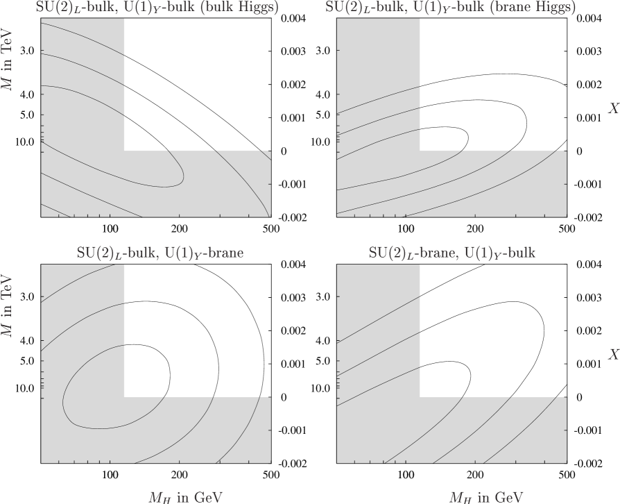
Figure 1: Contours of $\Delta\chi^{2}=1,\,4,\,9$ (eq. 3.2) derived from multi-parameter fits to electroweak precision data. The shaded regions of the parameter space correspond to $m_{H}<114$ GeV and/or $M^{2}<0$.

	brane-bulk	bulk-brane	bulk-bulk (brane Higgs)	bulk-bulk (bulk Higgs)
one-parameter fit	4.9	3.2	5.5	4.2
multi-parameter fit	3.1	3.1	4.2	3.7

Table 1: 2$\sigma$ bounds on $M$ in TeV derived from electroweak precision measurements [13].

Having described the methods, we will now discuss the resulting bounds on the compactification scale $M$ listed in Table 1. Superseding the one-parameter fit in [11], we use the latest experimental data [13] and take into account the error correlations which had previously been ignored. The error correlations have only a small effect, shifting the bounds by no more than 0.2 TeV. However, the change in the data with respect to the data of the year 2000 alters the bounds by as much as 1 TeV. This mainly is due to the large shift of the experimental value for the forward-backward asymmetry $A^{(0,b)}_{FB}$ which is now found to be more than 3$\sigma$ below the SM expectation. Only the bulk-bulk model with a bulk Higgs predicts a smaller value of $A^{(0,b)}_{FB}$ than the SM. Correspondingly, the bound for this model is lowered while the constraints on the other models become stronger.

In the multi-parameter fit, the correlations between $M$ and the SM parameters reduce the bounds as expected, the size of the effect varying from model to model. In the brane-bulk model the effect is biggest lowering the bound by almost 40%. Here, the best fit value is relatively far in the unphysical region. Thus, as a cross-check, we also performed a Bayesian analysis leading to a bound which is 0.1 TeV below the bound from (3.2).

Most interesting is the correlation between the compactification scale and the mass of the Higgs boson. This correlation is illustrated in Fig. 1. The data set used for this analysis differs from the one used for the familiar blue-band plot [22]. Within the SM ($X=0$ in Fig. 1) it leads to a best fit value $m_{H}=100^{+70}_{-40}$ GeV and to the 2$\sigma$ upper bound $m_{H}<280$ GeV. As can be seen in Fig. 1, in all models with the Higgs field localized on the brane, the existence of an extra dimension favors a heavier Higgs boson. This confirms the observation for the bulk-bulk model in [12]. The effect is most pronounced in the bulk-bulk model with a brane Higgs and in the brane-bulk model. Quantitatively, for $M=5$ TeV, the best fit values increase to $m_{H}=170^{+105}_{-60}$ GeV and $m_{H}=155^{+105}_{-60}$ GeV, respectively. If the compactification scale is included in the multi-parameter fit, the 2$\sigma$ upper bound on $m_{H}$ is relaxed to 330 and 400 GeV, respectively.

4 LEP2 Constraints

At energies above the $Z$ pole, the virtual exchange of KK excitations of the SM gauge bosons becomes dominant. As long as $s\ll M^{2}$, the main effects come from the interference of zero with higher KK modes. These effects scale like $s/M^{2}$ in contrast to the energy-independent modifications of masses and couplings, as is illustrated in Fig. 2 for muon-pair production. The residual energy dependence of the impact of the latter on the cross section (dashed curves in Fig. 2) is due to the transition from dominant $Z$ exchange to dominant photon exchange.

Focusing on LEP2, we have investigated the total cross sections for lepton-pair production, hadron production, and Bhabha scattering. Forward-backward asymmetries for muon and tau production as well as the heavy quark observables $A^{(0,b)}_{FB}$, $A^{(0,c)}_{FB}$, $R_{b}=\sigma(b\overline{b})/\sigma({\mathrm{had}})$, and $R_{c}=\sigma(c\overline{c})/\sigma({\mathrm{had}})$ are included in the fits, although they do not contribute noticeably to the bounds. For completeness, we have also investigated $W^{+}W^{-}$ production.

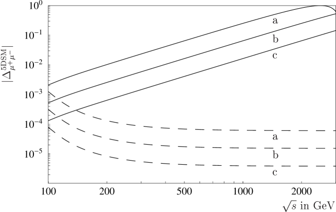
Figure 2: The shift $\Delta^{{\mathrm{5DSM}}}_{\mu^{+}\mu^{-}}$ of the total cross section for muon-pair production in the bulk-bulk model with a brane Higgs for $M=5$ (a), 10 (b), and 20 (c) TeV. The dashed curves show the effects from the mixing of masses and couplings only.

4.1 Fermion-Pair Production

The differential cross section for fermion-pair production is given by

$$\begin{split}\frac{d\,\sigma(e^{+}e^{-}\to f\,\overline{f})}{d\,\cos\vartheta}=\frac{N_{f}s}{128\,\pi}&\left[(1+\cos\vartheta)^{2}\,(|M^{ef}_{LL}(s)|^{2}+|M^{ef}_{RR}(s)|^{2})\,\,+\right.\\ &\,\,\,\left.(1-\cos\vartheta)^{2}\,(|M^{ef}_{LR}(s)|^{2}+|M^{ef}_{RL}(s)|^{2})\right]\,,\end{split}$$ (4.1)

where $\vartheta$ is the scattering angle between the incoming electron and the negatively charged outgoing fermion, and $N_{f}=1(3)$ for leptons (quarks) in the final state. For the matrix elements entering (4.1) one finds

$$M^{ef}_{\alpha\beta}(s)=\sum_{n=0}^{\infty}{\left(\,e_{(n)}^{2}\,\frac{Q_{e}Q_{f}}{s-m^{2}_{\gamma(n)}}\,+\,\frac{g^{e}_{\alpha(n)}g^{f}_{\beta(n)}}{\cos^{2}\theta_{W}}\,\frac{1}{s-m^{2}_{Z(n)}}\,\right)}$$ (4.2)

with the couplings

$$g^{f}_{L,R(n)}=\frac{g_{Z(n)}}{2}\left(g_{V(n)}\pm g_{A(n)}\right)\,$$ (4.3)

derived from (2.16), (2.18), and (2.19). The expression (4.1) has also been used in [23]. However, the mixing effects in the couplings and masses included in (4.2) and (4.3) have been neglected there.

	brane-bulk	bulk-brane	bulk-bulk (brane Higgs)	bulk-bulk (bulk Higgs)
$\mu^{+}\mu^{-}$	2.0	1.5	2.5	2.5
$\tau^{+}\tau^{-}$	2.0	1.5	2.5	2.5
hadrons	2.6	4.7	5.4	5.8
$e^{+}e^{-}$	3.0	2.0	3.6	3.5
$W^{+}W^{-}$	1.1	2.0	2.1	2.2
LEP2 combined	3.5	4.6	5.6	5.9
Electroweak and LEP2 data combined	5.4	4.8	6.9	6.0

Table 2: 2$\sigma$ bounds on $M$ in TeV from a one-parameter fit derived from LEP2 data alone and from LEP2 and electroweak precision data combined.

The data taken by the LEP experiments for muon, tau, and hadron production is properly combined in [22] for energies between $\sqrt{s}=130\,{\mathrm{GeV}}$ and $\sqrt{s}=207\,{\mathrm{GeV}}$. In the hadronic channel it is very important to take into account the large correlations between the data at different energies. If they are ignored, the bounds on the compactification scale are overestimated by as much as 3 TeV. On the other hand, correlations in the muon and tau channels are extremely small and have little effect.

The bounds from a simple one-parameter analysis are summarized in Table 2. In the muon and tau channel, the bulk-brane model is least restricted because essentially only left-handed fermions interact with the KK modes. The best fit values turn out to lie always in the physical region $X\geq 0$. Hadron production puts more stringent bounds on the 5D models because of the larger cross section. In this case, the brane-bulk model is least restricted, since the hadronic cross section is dominated by left-handed quarks whose small hypercharges suppress the interference effects with the U(1)_Y KK modes. In this case, the best fit values lie in the unphysical region $X<0$.

The differential cross section for Bhabha scattering may conveniently be expressed as

$$\begin{split}\frac{d\,\sigma(e^{+}e^{-}\to e^{+}e^{-})}{d\,\cos\vartheta}=&\frac{s}{128\,\pi}\left[(1+\cos\vartheta)^{2}\,(|M^{ee}_{LL}(s)+M^{ee}_{LL}(t)|^{2}+|M^{ee}_{RR}(s)+M^{ee}_{RR}(t)|^{2})\,\,+\right.\\ &\left.(1-\cos\vartheta)^{2}\,(|M^{ee}_{LR}(s)|^{2}+|M^{ee}_{RL}(s)|^{2})+4\,(|M^{ee}_{LR}(t)|^{2}+|M^{ee}_{RL}(t)|^{2})\right],\end{split}$$ (4.4)

where $t=-s(1-\cos\vartheta)/2$ and $M^{ee}_{\alpha\beta}(s\,\mathrm{or}\,t)$ can be read off from (4.2). The total cross section is calculated by integrating (4.4) over $\vartheta$ in the experimental ranges. Since the Bhabha data of the four LEP experiments [24] has not yet been combined, possible correlations of the different experiments cannot be accounted for, at least for the time being.

As can be seen from Table 2, the bounds on $M$ from Bhabha scattering are approximately 1 TeV stronger than those from the other leptonic channels. This is due to the large Bhabha cross section. On the other hand, the dominance of the $t$-channel photon exchange, which is not affected by the presence of an extra dimension, reduces the sensitivity of Bhabha scattering with respect to hadron production in almost all 5D models.

4.2 $W^{+}W^{-}$ Production

The differential cross section for $W^{+}W^{-}$ production reads [25]

$$\begin{split}&\frac{d\,\sigma(e^{+}e^{-}\to W^{+}\,W^{-})}{d\,\cos\vartheta}=\frac{1}{32\pi s}\,\beta\\[8.61108pt] &\,\times\left\{\beta^{2}{\left[\,M^{2}_{L}(s)+M^{2}_{R}(s)\,\right]}s^{2}{\left[\,\frac{s}{m_{W(0)}^{2}}+\sin^{2}\vartheta\,{\left(\,\frac{3}{4}-\frac{s}{4m_{W(0)}^{2}}+\frac{s^{2}}{16m_{W(0)}^{4}}\,\right)}\,\right]}\right.\\[8.61108pt] &\,\quad+M^{2}_{L}(t)t^{2}{\left[\,\frac{s}{4m_{W(0)}^{2}}+\beta^{2}\sin^{2}\vartheta{\left(\,\frac{s^{2}}{16t^{2}}+\frac{s^{2}}{64m_{W(0)}^{4}}\,\right)}\,\right]}\\[8.61108pt] &\left.\,\quad+M_{L}(t)M_{L}(s)\,st\,{\left[\,\!2+2\frac{m_{W(0)}^{2}}{t}+\beta^{2}\frac{s}{m_{W(0)}^{2}}-\beta^{2}\sin^{2}\vartheta{\left(\,\frac{s}{4t}+\frac{s}{8m_{W(0)}^{2}}-\frac{s^{2}}{16m_{W(0)}^{4}}\,\right)}\!\,\right]}\right\}\,,\end{split}$$ (4.5)

where $\beta=\sqrt{1-4m_{W(0)}^{2}/s}$, $t=m^{2}_{W(0)}-s\,(1-\sqrt{1-\beta}\,\cos\vartheta)/2$ and $\vartheta$ is the scattering angle between the electron and the negatively charged $W$ boson. Note, that $m_{W(0)}=m_{W}^{{\mathrm{SM}}}\,{\left(\,1+\Delta_{m_{W}}X\,\right)}$ with

$$\Delta_{m_{W}}=\bigg{\{}\ \frac{1}{2}\,s^{4}_{\beta}\hat{s}^{2}_{W}\,-\,\frac{\hat{s}^{2}_{W}\hat{c}^{2}_{W}}{2\hat{c}_{2W}}\,\bigg{(}\,1\>-\>2s^{2}_{\beta}\>-\>\frac{\hat{s}^{2}_{W}}{\hat{c}^{2}_{W}}s^{4}_{\beta}\,\bigg{)}\,,\quad\frac{\hat{s}^{2}_{W}\hat{c}^{2}_{W}}{2\,\hat{c}_{2W}}\,,\quad\frac{\hat{s}^{2}_{W}\hat{c}^{2}_{W}}{2\,\hat{c}_{2W}}\,\bigg{\}}\,$$ (4.6)

for the bulk-bulk, the brane-bulk, and the bulk-brane model, respectively [11]. Furthermore, $M_{L,R}(s)$ and $M_{L}(t)$ are given by

$$\begin{split}M_{\alpha}(s)&=\sum_{n=0}^{\infty}{\left(\,\frac{Q_{e}\,e_{(n)}\,g_{3(n)}^{\gamma}}{s-m^{2}_{\gamma(n)}}\,+\,\frac{g^{e}_{\alpha(n)}g^{Z}_{3(n)}}{\cos\theta_{W}}\,\frac{1}{s-m^{2}_{Z(n)}}\,\right)}\,,\\[8.61108pt] M_{L}(t)&=\frac{g^{2}_{W(0)}}{t}\,,\end{split}$$ (4.7)

while $M_{R}(t)=0$ as in the SM. A novel feature are the triple gauge-boson couplings $g_{3(n)}^{\gamma}$ and $g^{Z}_{3(n)}$ of the photon, the $Z$ boson, and their respective KK modes with the $W$ zero modes. They are given in Appendix A along with the corresponding Feynman rules.

As can be seen from Table 2, $W$-pair production at LEP2 provides relatively weak bounds on $M$. This can be understood by realizing that the effects of KK exchange are almost negligible due to the suppression of the interference of SM and KK exchange by an additional factor $X$. This is a direct consequence of selection rules which forbid the triple boson couplings of a single higher KK mode to zero modes for the gauge eigenstates such that they can only be induced by mixing.

Figure 3: Contours of $\Delta\chi^{2}=1,\,4,\,9$ (eq. 3.2) derived from the combined analysis of LEP2 data and electroweak precision measurements. The shaded regions of the parameter space correspond to $m_{H}<114$ GeV and/or $M^{2}<0$.

4.3 Combined Bounds on the compactification scale $M$

The 2$\sigma$ bounds on $M$ found from a one-parameter fit to the combined LEP2 data are listed in Table 2. The bounds range from 3.5 TeV for the brane-bulk model to 5.9 TeV for the bulk-bulk model with a bulk Higgs. Furthermore, including also the electroweak precision measurements, the bounds range from 4.8 TeV for the bulk-brane model to 6.9 TeV for the bulk-bulk model with a brane Higgs. For the bulk-bulk models our results agree with the results of [23]. The best fit values always lie in the unphysical region $X<0$.

For muon-pair, tau-pair and hadron production (including asymmetries and heavy-quark data), where ZFITTER can be used to calculate the SM predictions, we have also performed a multi-parameter fit. The resulting $\Delta\chi^{2}$ contours are shown in Fig. 3. The slight distortions from smooth contours are due to a discontinuity in hadronic cross sections and asymmetries found in ZFITTER version 6.36 at $\sqrt{s}=m_{t}$ [26]. The corresponding 2$\sigma$ bounds on $M$ are listed in Table 3 along with the bounds from the corresponding one-parameter fit. The correlations between $m_{H}$, $m_{t}$, and $M$ are similar to what has been found from the precision observables alone in Section 3. They are weak in the bulk-brane model and most sizable in the brane-bulk model.

A comparison of Table 2 and 3 shows that in the one-parameter fit Bhabha scattering and $W^{+}W^{-}$ production increase the combined bounds by about 0.5 TeV. Thus, the bounds from a multi-parameter fit to all data, including Bhabha scattering and $W^{+}W^{-}$ production can be estimated to lie between 4 TeV for the brane-bulk model and 6 TeV for the bulk-bulk model with a brane Higgs.

	brane-bulk	bulk-brane	bulk-bulk (brane Higgs)	bulk-bulk (bulk Higgs)
one-parameter fit	5.0	4.5	6.4	5.5
multi-parameter fit	3.6	4.3	5.4	5.2

Table 3: 2$\sigma$ bounds on $M$ in TeV derived from the muon-, tau-, and hadron production at LEP2 combined with electroweak precision measurements.

5 Sensitivity at a Linear Collider

Having extracted the bounds on the compactification scale $M$ from available data, we will now estimate the reach at a future linear collider such as TESLA [27]. For illustration, we investigate both the potential of the GigaZ option as well as the sensitivity at high energy and luminosity.

5.1 GigaZ option

At the $Z$ pole, the luminosity goal at TESLA is $\mathcal{L}=5\times 10^{33}$ cm^-2 s^-1 which is sufficient to produce $10^{9}$ $Z$ bosons in only 50-100 days of running [27]. This will increase the LEP statistics by more than an order of magnitude. The most relevant improvement in testing the compactification scale will come from the precise measurement of the left-right (LR) asymmetry $A_{\mathrm{LR}}$. Since photon exchange and the exchange of higher KK modes can be neglected on the $Z$ peak, the LR asymmetry at tree level can be approximated by

$$A_{\mathrm{LR}}\ =\ \frac{2\,g_{V(0)}\,g_{A(0)}}{g_{V(0)}^{2}\>+\>g_{A(0)}^{2}}\,,$$ (5.1)

where $g_{V(0)}$ and $g_{A(0)}$ are the vector and axial vector couplings of the electron to the $Z$ boson given in (2.16). This asymmetry is very sensitive to shifts of the weak mixing angle with respect to the SM value because of the small ratio $g_{V}/g_{A}=(1-4\sin^{2}\theta_{W})$. Using (2.10) and (2.18) in order to express (5.1) in terms of the input parameters, one obtains the 5DSM corrections $\Delta_{A_{\mathrm{LR}}}=\Delta_{A_{e}}$ given in [11].

With the GigaZ option it will be possible to measure $A_{\mathrm{LR}}$ with an absolute error of about $10^{-4}$ [27]. However, the uncertainties in the fine structure constant and the $Z$ mass will each induce an additional error of about $10^{-4}$ which has to be added in quadrature. Coincidence of the measured value of $A_{\mathrm{LR}}$ with the SM expectation would then imply the bounds on $M$ shown in Table 4. As can be seen, except for the bulk-brane model, the GigaZ option should allow to improve the existing bounds by at least a factor 2.

With excellent $b$-tagging, it will also be possible to considerably improve the measurement of the final state coupling $A_{b}$ and the cross-section ratio $R_{b}$. The experimental error for the mass of the $W$ boson can also be reduced significantly by a threshold scan. However, the sensitivity of these observables to $M$ is small and does not allow to explore compactification scales beyond the bounds already known from available data.

	brane-bulk	bulk-brane	bulk-bulk (brane Higgs)	bulk-bulk (bulk Higgs)
$A_{\mathrm{LR}}$	12.4	6.8	14.2	12.4

Table 4: 2$\sigma$ bound on the compactification scale $M$ in TeV which can be obtained with the GigaZ option at TESLA if the measured value of $A_{\mathrm{LR}}$ coincides with the SM expectation.

5.2 Tests at $\sqrt{s}=800$ GeV

At high energies, the interference effects from the exchange of SM and KK modes completely dominate the mixing effects as illustrated in Fig. 2. We consider the same processes as in Section 4, except for $W$-pair production which is not very sensitive to an extra dimension since the couplings of the $W$ bosons to higher KK modes in the $s$-channel are either forbidden or suppressed. For Bhabha scattering, an acceptance cut, $|\cos\vartheta|<0.9$, is included. Furthermore, we assume an integrated luminosity of 1000 fb^-1.

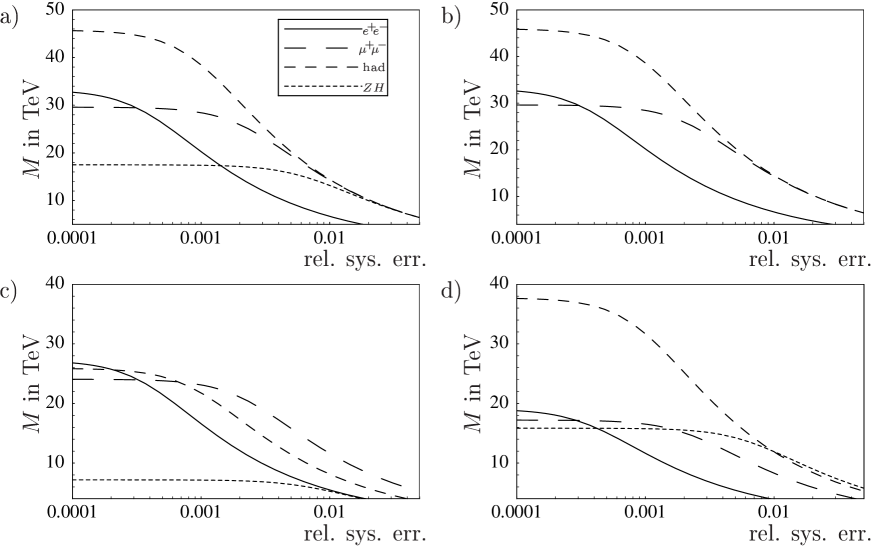
Figure 4: Expected sensitivity to $M$ as a function of relative systematic error at $\sqrt{s}=800$ GeV and for an integrated luminosity of 1000 fb^-1: (a) bulk-bulk model with brane Higgs, (b) bulk-bulk model with bulk Higgs, (c) brane-bulk model, and (d) bulk-brane model.

In addition, we also study Higgsstrahlung, the differential cross section of which is given by

$$\frac{d\,\sigma(e^{+}e^{-}\to Z\,H)}{d\,\cos\vartheta}\ =\ \frac{s}{512\pi}\,\lambda^{1/2}(s)\,{\left[\,8\frac{m_{Z(0)}^{2}}{s}\>+\>\lambda(s){\left(\,1-\cos^{2}\vartheta\,\right)}\,\right]}\,{\left[\,M_{L}^{2}(s)+M_{R}^{2}(s)\,\right]}\,.$$ (5.2)

Here, $\lambda(s)=\!{\left(\,\!1-{\left(\,m_{H}+m_{Z(0)}\,\right)}^{2}/s\,\right)}{\left(\,\!1-{\left(\,m_{H}-m_{Z(0)}\,\right)}^{2}/s\,\right)}$ is the familiar two-particle phase-space function, $\vartheta$ is the scattering angle between the electron and the outgoing $Z$, and

$$M_{\alpha}(s)=\sum_{n=0}^{\infty}{\left(\,\frac{g^{e}_{\alpha(n)}\,\,g^{ZH}_{(n)}}{\cos^{2}\theta_{W}}\frac{1}{s-m^{2}_{Z(n)}}\,\right)}\,.$$ (5.3)

The couplings $g^{e}_{\alpha(n)}$ are defined in (4.3) and $g^{ZH}_{(n)}$ is the effective coupling of the $Z$ modes to the Higgs boson given in Appendix B. The integrated cross section following from (5.2) in the SM limit can be found, for example, in [28].

The Higgsstrahlung process is certainly not a primary search channel for an extra dimension because of the limited experimental accuracy. For $\int\!\mathcal{L}\,dt=10^{3}$ fb^-1 and at $\sqrt{s}=800$ GeV, the error on the total cross section for $m_{H}\simeq 115$ GeV is expected to be 5% [27]. Nevertheless, this channel is interesting for distinguishing between a brane and a bulk Higgs in the bulk-bulk model. If the produced Higgs boson is the zero mode of a bulk field, the KK selection rules forbid the coupling $H_{(0)}Z_{(0)}Z_{(n)}$ for $n\geq 1$. Thus, the absence of massive KK-modes in the s-channel is a clear signal for a bulk Higgs. In this case, this process is rather SM-like in contrast to a Higgs boson localized on the brane. The phenomenology of 2-Higgs-doublet models with a bulk and a brane Higgs has been investigated in [29].

Figure 5: Combined sensitivity to the compactification scale $M$ as a function of relative systematic error at $\sqrt{s}=800$ GeV and for an integrated luminosity of 1000 fb^-1 in the models bulk-bulk with brane Higgs (short dashed), bulk-bulk with bulk Higgs (solid), brane-bulk (dashed), and bulk-brane (long dashed).

In the following, the sensitivity to the presence of an extra dimension is estimated by requiring

$$\chi^{2}=\sum_{i}\,\frac{{\left(\,\mathcal{O}_{i}^{{\mathrm{SM}}}\>-\>\mathcal{O}_{i}^{{\mathrm{5DSM}}}\,\right)}^{2}}{(\Delta\mathcal{O}_{i})^{2}}\,\leq\,4\,.$$ (5.4)

The statistical errors will be so small that the systematic errors become decisive [30, 31]. Since the latter are not reliably known at the present time, we show, in Fig. 4, the sensitivity to the compactification scale $M$ as a function of the relative systematic error. At $\Delta\mathcal{O}_{\mathrm{sys}}\stackrel{{\scriptstyle<}}{{{}_{\sim}}}0.001$ the statistical uncertainty begins to dominate and the sensitivity to the compactification scale saturates.

The combined sensitivity of the search channels of Fig. 4 is presented in Fig. 5. For bulk/brane (bulk/bulk) models, the sensitivity limit increases from 15 (20) TeV for systematic errors at the 1% level to 35 (50) TeV for negligible systematic errors. The role played by the statistics is illustrated in Fig. 6, where the combined sensitivity is plotted as a function of integrated luminosity.

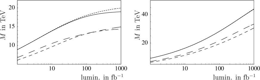
Figure 6: Search limit as a function of the integrated luminosity at $\sqrt{s}~{}=~{}800$ GeV assuming a systematic error of 1.0% (left) and 0.1% (right). Combination of channels, and models as in Fig. 5.

In addition to integrated cross sections, it is also interesting to study the effects of an extra dimension on angular distributions. This may provide further handles to discriminate between different models. For the muon and tau channel, the angular distribution in the bulk-bulk model is almost completely SM-like. However, the brane-bulk and the bulk-brane models lead to significant distortions of the angular distribution because of the almost pure U(1)_Y and SU(2)_L nature of the heavy KK modes. In Bhabha scattering, the $s$- and the $t$-channel are affected differently such that the angular distribution is also affected in the bulk-bulk models.

For illustration, Fig. 7 shows the shift $\Delta^{\mathrm{5DSM}}_{\mathrm{\vartheta}}$ of $(d\sigma/d\cos\vartheta)/\sigma_{\mathrm{tot}}$ from the SM prediction as defined in (2.5). If the angular distributions in the muon channel can be measured with a precision better than 1% per bin (using ten bins), one can probe the compactification scale $M$ beyond 10 TeV for the brane-bulk and the bulk-brane model. In Bhabha scattering, one can reach a similar scale also for the bulk-bulk models, while the bulk-brane model is difficult to probe in this channel.

6 Conclusions

In this article, we have determined detailed and robust bounds on the compactification scale $M$ from electroweak precision data and LEP2 measurements of fermion and W pair production. Our analysis includes correlations of experimental errors in the data. Moreover, besides one-parameter fits, we have performed multi-parameter fits in order to include correlations between the SM parameters and the compactification scale $M$. In addition, we have estimated the sensitivity to $M$ at a future $e^{+}e^{-}$ collider such as TESLA. For this estimate, we have considered fermion-pair production and Higgsstrahlung.

Figure 7: Deviation of the angular distribution $(d\sigma/d\cos\vartheta)/\sigma_{\mathrm{tot}}$ in muon-pair production (left) and Bhabha scattering (right) from the SM predictions for $M~{}=~{}10$ TeV in the bulk-bulk (solid), brane-bulk (dashed), and bulk-brane (long dashed) models.

If both the SU(2)_L and U(1)_Y fields are bulk fields, the existing data imply $M>5.5-6$ TeV where the range reflects the dependence on details of the Higgs sector. If the SU(2)_L or U(1)_Y fields are confined to the brane where the fermions live the bounds are $M>4$ TeV and $M>5$ TeV, respectively. Furthermore, we have shown that the presence of an extra compact dimension relaxes the upper bound on the SM Higgs mass from 280 GeV in the SM (for the data set used in Section 3) to 400 GeV and 330 GeV in the brane-bulk and the bulk-bulk model with a brane Higgs, respectively.

At an $e^{+}e^{-}$ linear collider, the GigaZ option should allow to increase the sensitivity to $M$ by a factor 2 in almost all 5D models. At $\sqrt{s}=800$ GeV and for an integrated luminosity of 1000 fb^-1 the discovery potential will crucially depend on the control of systematic errors. For a systematic uncertainty of 1% in each search channel, one will be able to reach compactification scales in the range 15-20 TeV. For systematic uncertainties smaller than the statistical uncertainties, the sensitivity limit is estimated to be in the range $M=$ 35-50 TeV.

Finally, for a sufficiently low compactification scale, $M\stackrel{{\scriptstyle<}}{{{}_{\sim}}}10$ TeV, Higgsstrahlung and angular distributions of 2-fermion final states can be used to discriminate between different 5D models. In particular, Higgsstrahlung can be used to distinguish brane from bulk Higgs bosons.

Acknowledgements

This work was supported in part by the Bundesministerium für Bildung und Forschung (BMBF, Bonn, Germany) under contract 05HT1WWA2, the Studienstiftung des deutschen Volkes, and PPARC grant number PPA/G/O/2000/00461. We wish to thank the participants of the Heidelberg theory colloquium for an inspiring discussion and G. Quast for his help with ZFITTER.

Appendix A Kaluza–Klein $W_{(0)}W_{(0)}Z_{(n)}$ and $W_{(0)}W_{(0)}\gamma_{(n)}$ couplings

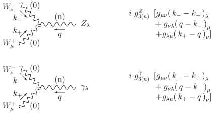
Figure 8: Triple gauge boson couplings. The numbers in parenthesis denote the KK mode numbers.

Here, we present the Feynman rules for the triple gauge boson vertices shown in Fig. 8. In the gauge basis, only the $W^{+}_{(0)}W^{-}_{(0)}Z_{(0)}$ and $W^{+}_{(0)}W^{-}_{(0)}\gamma_{(0)}$ vertices exist while the vertices $W^{+}_{(0)}W^{-}_{(0)}Z_{(n)}$ and $W^{+}_{(0)}W^{-}_{(0)}\gamma_{(n)}$ with $n\geq 1$ are forbidden by KK selection rules [11, 32]. However, in the mass eigenstate basis, couplings to heavy KK states are induced by the diagonalization of the gauge-boson mass matrix. Below, we give these couplings to first order in $X$. To this order the zero-mode couplings are unaffected, that is

$$g^{Z}_{3(0)}=g\,\cos\theta_{W}\,,\quad\quad g^{\gamma}_{3(0)}=e\,$$ (A.1)

with $g$ from (2.9). For the higher modes ($n\geq 1$), one gets

$$g^{Z}_{3(n)}=\sqrt{2}\,e\,\frac{\hat{c}_{W}}{\hat{s}_{W}}\,{\left(\,\hat{s}_{W}^{2}-\hat{c}_{W}^{2}\,\right)}\,s^{2}_{\beta}\,\frac{3}{n^{2}\pi^{2}}\,X\,$$ (A.2)

$$g^{\gamma}_{3(n)}=-\sqrt{2}\,e\,\hat{c}^{2}_{W}\,s^{2}_{\beta}\,\frac{6}{n^{2}\pi^{2}}\,X\,$$ (A.3)

in the bulk-bulk model,

$$g^{Z}_{3(n)}=\sqrt{2}\,e\,\hat{c}_{W}\,\frac{3}{n^{2}\pi^{2}}\,X\,$$ (A.4)

in the brane-bulk model, and

$$g^{Z}_{3(n)}=-\sqrt{2}\,e\,\frac{\hat{c}^{2}_{W}}{\hat{s}_{W}}\,\frac{3}{n^{2}\pi^{2}}\,X\,$$ (A.5)

in the bulk-brane model. In the latter two models, the $\gamma_{(n)}$ modes for $n\geq 1$ are absent.

Appendix B Kaluza–Klein $H_{(0)}Z_{(0)}Z_{(n)}$ couplings

In the bulk-bulk model with a brane Higgs only, the $HZZ$ coupling can be derived in the gauge basis from

$$\begin{split}{\mathcal{L}}_{{\mathrm{HZZ}}}(x)&=\frac{1}{4}\frac{g^{2}v}{c_{W}^{2}}\,h\,{\left(\,Z_{(0)}^{\mu}+\sum_{n=1}^{\infty}\sqrt{2}\,Z_{(n)}^{\mu}\,\right)}^{2}\\ &=\frac{g}{2}\,\frac{m_{Z(0)}}{c_{W}}\left(1-\frac{\Delta_{Z}}{2}X\right)\,h\,{\left(\,Z_{(0)}^{\mu}+\sum_{n=1}^{\infty}\sqrt{2}\,Z_{(n)}^{\mu}\,\right)}^{2}\,,\end{split}$$ (B.1)

where $h$ denotes the Higgs field on the brane and $v$ its VEV. The second relation follows from (2.7). In the bulk-bulk model with a bulk Higgs field, the KK selection rules forbid the couplings of two zero modes to higher modes. Moreover, the gauge eigenstates coincide with the mass eigenstates. Thus, for zero-mode final states, Higgsstrahlung is described by the same $H_{(0)}Z_{(0)}Z_{(0)}$ vertex as in the SM. In the brane-bulk or bulk-brane model, the $Z_{(n)}^{\mu}$ tower coincides with the U(1)_Y or SU(2)_L KK modes for $n\geq 1$, respectively. Because a brane Higgs field breaks momentum conservation in the extra dimension, no selection rules exist.

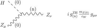
Figure 9: The $HZZ$ vertex. The numbers in parenthesis specify the KK modes.

In the mass eigenstate basis, the Lagrangian (B.1) leads to the vertex shown in Fig. 9. In summary, the effective couplings are given by

$$g^{{\mathrm{ZH}}}_{(0)}=g\quad\quad{\mathrm{and}}\quad\quad g^{{\mathrm{ZH}}}_{(n\geq 1)}=0$$ (B.2)

in the bulk-bulk model with a bulk Higgs,

$$\begin{split}g^{{\mathrm{ZH}}}_{(0)}\,&=\,g\,\left[1\,-\,\left(2+\frac{\Delta_{Z}}{2}\right)\,X\right]\,,\\[8.61108pt] g^{{\mathrm{ZH}}}_{(n\geq 1)}\,&=\,\sqrt{2}\,g\,{\left[\,1\,-\,{\left(\,1+\frac{3}{2\,n^{2}\pi^{2}}+\frac{\Delta_{Z}}{2}\,\right)}\,X\,\right]}\,,\end{split}$$ (B.3)

in the bulk-bulk model with a brane Higgs,

$$\begin{split}g^{{\mathrm{ZH}}}_{(0)}\,&=\,g\,\left[1\,-\,\left(2\,\hat{s}_{W}^{2}+\frac{\Delta_{Z}}{2}\right)\,X\right]\,,\\[8.61108pt] g^{{\mathrm{ZH}}}_{(n\geq 1)}\,&=\,\sqrt{2}\,s_{W}\,g\,{\left[\,1\,-\,{\left(\,\hat{s}_{W}^{2}+{\left(\,3\,\hat{s}_{W}^{2}\,-\,2\,\right)}\frac{3}{2\,n^{2}\pi^{2}}+\frac{\Delta_{Z}}{2}\,\right)}\,X\,\right]}\,,\end{split}$$ (B.4)

in the brane-bulk model, and

$$\begin{split}g^{{\mathrm{ZH}}}_{(0)}\,&=\,g\,\left[1\,-\,\left(2\,\hat{c}_{W}^{2}+\frac{\Delta_{Z}}{2}\right)\,X\right]\,,\\[8.61108pt] g^{{\mathrm{ZH}}}_{(n\geq 1)}\,&=\,\sqrt{2}\,c_{W}\,g\,{\left[\,1\,-\,{\left(\,\hat{c}_{W}^{2}+{\left(\,3\,\hat{c}_{W}^{2}\,-\,2\,\right)}\frac{3}{2\,n^{2}\pi^{2}}+\frac{\Delta_{Z}}{2}\,\right)}\,X\,\right]}\,,\end{split}$$ (B.5)

in bulk-brane model. The factor $\sqrt{2}$ in $g^{{\mathrm{ZH}}}_{(n\geq 1)}$ is the usual enhancement of couplings between higher KK modes and brane fields. The factors $s_{W}$ and $c_{W}$ reflect the fact that for $n\geq 1$ $Z_{(n)}^{\mu}$ is mainly $B^{\mu}_{(n)}$ or $A^{3\mu}_{(n)}$, respectively.

References

- [1] T. Kaluza, Sitzungsber. d. Preuss. Akad. d. Wiss. Berlin, (1921) 966; O. Klein, Z. Phys. 37 (1926) 895.
- [2] I. Antoniadis, Phys. Lett. B246 (1990) 377; J.D. Lykken, Phys. Rev. D54 (1996) 3693.
- [3] E. Witten, Nucl. Phys. B471 (1996) 135; P. Hoava and E. Witten, Nucl. Phys. B460 (1996) 506; Nucl. Phys. B475 (1996) 94.
- [4] N. Arkani-Hamed, S. Dimopoulos, and G. Dvali, Phys. Lett. B429 (1998) 263; Phys. Rev. D59 (1999) 086004; I. Antoniadis, N. Arkani-Hamed, S. Dimopoulos, and G. Dvali, Phys. Lett. B436 (1998) 257.
- [5] K.R. Dienes, E. Dudas, and T. Gherghetta, Phys. Lett. B436 (1998) 55; Nucl. Phys. B537 (1999) 47.
- [6] G.F. Giudice, R. Rattazzi, and J.D. Wells, Nucl. Phys. B544 (1999) 3; T. Han, J.D. Lykken, and R.-J. Zhang, Phys. Rev. D59 (1999) 105006; E.A. Mirabelli, M. Perelstein, and M.E. Peskin, Phys. Rev. Lett. 82 (1999) 2236; J.L. Hewett, Phys. Rev. Lett. 82 (1999) 4765; T.G. Rizzo, Phys. Rev. D59 (1999) 115010.
- [7] L.J. Hall and D.R. Smith, Phys. Rev. D60 (1999) 085008.
- [8] T. Appelquist, H.C. Cheng, and B.A. Dobrescu, Phys. Rev. D64 (2001) 035002.
- [9] K. Agashe, N.G. Deshpande, and G.H. Wu, Phys. Lett. B514 (2001) 309; C. Macesanu, C.D. McMullen, and S. Nandi, Phys. Rev. D66 (2002) 015009; T.G. Rizzo, Phys. Rev. D64 (2001) 095010; F.J. Petriello, JHEP 0205 (2002) 003; A.J. Buras, M. Spranger, and A. Weiler, Nucl. Phys. B660 (2003) 225; P. Bucci and B. Grzadkowski, Phys. Rev. D64 (2003) 124002; P. Dey and G. Bhattacharyya, hep-ph/0309110.
- [10] J. Papavassiliou and A. Santamaria, Phys. Rev. D63 (2001) 016002; J.F. Oliver, J. Papavassiliou, and A. Santamaria, Phys. Rev. D67 (2003) 056002.
- [11] A. Mück, A. Pilaftsis, and R. Rückl, Phys. Rev. D65 (2002) 085037.
- [12] T. Rizzo and J. Wells, Phys. Rev. D61 (2000) 016007; A. Strumia, Phys. Lett. B466 (1999) 107.
- [13] Particle Data Group (K. Hagiwara et al.), Phys. Rev. D66 (2002) 010001.
- [14] B.W. Lee, C. Quigg, and H.B. Thacker, Phys. Rev. D16 (1977) 1519.
- [15] J. Polchinski, Phys. Rev. Lett. 75 (1995) 4724.
- [16] M. Berkooz, M.R. Douglas, and R.G. Leigh, Nucl. Phys. B480 (1996) 265.
- [17] G. Aldazábal, L.E. Ibáez, F. Quevedo, and A.M. Uranga, JHEP 0008 (2000) 002; G. Aldazábal, S. Franco, L.E. Ibáez, R. Rabadán, and A.M. Uranga, J. Math. Phys. 42 (2001) 3103; JHEP 0102 (2001) 047; R. Blumenhagen, B. Körs, D. Lüst, and T. Ott, Nucl. Phys. B616 (2001) 3; M. Cveti, G. Shiu, and A.M. Uranga, Phys. Rev. Lett. 87 (2001) 201801; D. Bailin, G.V. Kraniotis, and A. Love, Phys. Lett. B530 (2002) 202; L.L. Everett, G.L. Kane, S.F. King, S. Rigolin, and L.T. Wang, Phys. Lett. B531 (2002) 263; D. Cremades, L.E. Ibáez, and F. Marchesano, JHEP 0207 (2002) 022; G. Honecker, JHEP 0201 (2002) 025; C. Kokorelis, JHEP 0208 (2002) 036; J.R. Ellis, P. Kanti, and D.V. Nanopoulos, Nucl. Phys. B647 (2002) 235.
- [18] H. Georgi, A.K. Grant, and G. Hailu, Phys. Lett. B506 (2001) 207; G.V. Gersdorff, N. Irges, and M. Quirós, Nucl. Phys. B635 (2002) 127; M. Carena, T.M.P. Tait, and C.E.M. Wagner, Acta Phys. Polon. B33 (2002) 2355.
- [19] D. Bardin et al., Z. Phys. C44 (1989) 493; Comp. Phys. Comm. 59 (1990) 303; Nucl. Phys. B351 (1991) 1; Phys. Lett. B255 (1991) 290; Comp. Phys. Comm. 133 (2001) 229.
- [20] F. James and M. Roos, Comput. Phys. Commun. 10 (1975) 343.
- [21] G.J. Feldman and R.D. Cousins, Phys. Rev. D57 (1998) 3873.
- [22] The LEP Collaborations ALEPH, DELPHI, L3, OPAL, the LEP Electroweak Working Group, and the SLD Heavy Flavor and Electroweak Groups, hep-ex/0112021.
- [23] K. Cheung and G. Landsberg, Phys. Rev. D65 (2002) 076003.
-
[24]
The ALEPH collaboration, Eur. Phys. J. C12 (2000) 183; ALEPH 99-018; ALEPH 2000-25; ALEPH 2001-019.
The DELPHI collaboration, Eur. Phys. J. C11 (1999) 383; Phys. Lett. B485 (2000) 45; DELPHI 2000-128; DELPHI 2001-094.
The L3 collaboration, Phys. Lett. B479 (2000) 101.
The OPAL collaboration, Eur. Phys. J. C2 (1998) 441; Eur. Phys. J. C6 (1999) 1; Eur. Phys. J. C13 (2000) 553; OPAL PN 424 (2000); OPAL PN 469 (2001).
- [25] W. Alles, C. Boyer, and A.J. Buras, Nucl. Phys. B119 (1977) 125.
- [26] Private communication with D. Bardin.
- [27] TESLA-Technical Design Report, DESY-2001-011, hep-ph/0106315.
- [28] W. Kilian, M. Krämer, and P. Zerwas, Phys. Lett. B373 (1996) 135.
- [29] A. Aranda, C. Balázs, and J.L. Diaz-Cruz, Nucl. Phys. B670 (2003) 90.
- [30] S. Riemann, LC-TH-2001-007 in 2nd ECFA/DESY Study 1998-2001, (2001) 1451.
- [31] D. Bourilkov, Contribution to LHC/LC Study Group Working Document, hep-ph/0305125.
- [32] D. Dicus, C. McMullen, and S. Nandi, Phys. Rev. D65 (2002) 076007.