Nonequilibrium pion dynamics near the critical point in a constituent quark model

Abstract

We study static and dynamical critical phenomena of chiral symmetry breaking in a two-flavor Nambu–Jona-Lasinio constituent quark model. We obtain the low-energy effective action for scalar and pseudoscalar degrees of freedom to lowest order in quark loops and to quadratic order in the meson fluctuations around the mean field. The static limit of critical phenomena is shown to be described by a Ginzburg-Landau effective action including spatial gradients. Hence static critical phenomena is described by the universality class of the O(4) Heisenberg ferromagnet. Dynamical critical phenomena is studied by obtaining the equations of motion for pion fluctuations. We find that for $T<T_{c}$ the are stable long-wavelength pion excitations with dispersion relation $\omega_{\pi}(k)=k$ described by isolated pion poles. The residue of the pion pole vanishes near $T_{c}$ as $Z\propto 1/|\ln(1-T/T_{c})|$ and long-wavelength fluctuations are damped out by Landau damping on a time scale $t_{\mathrm{rel}}(k)\propto 1/k$, reflecting critical slowing down of pion fluctuations near the critical point. At the critical point, the pion propagator features mass shell logarithmic divergences which we conjecture to be the harbinger of a (large) dynamical anomalous dimension. We find that while the classical spinodal line coincides with that of the Ginzburg-Landau theory, the growth rate of long-wavelength spinodal fluctuations has a richer wavelength dependence as a consequence of Landau damping. We argue that Landau damping prevents a local low energy effective action in terms of a derivative expansion in real time at least at the order studied.

I Introduction

The spontaneous breaking of chiral symmetry in the QCD vacuum has fundamental significance in understanding the nonperturbative nature of hadron dynamics. In QCD with two massless quark flavors at zero baryon density, the chiral phase transition is expected to be second order and to be described by the universality class of the three-dimensional O(4) Heisenberg model pisarski ; wilraja . Recent lattice simulations for two-flavor QCD in the chiral limit at finite temperature and vanishing baryon chemical potential seems to indicate that chiral symmetry is restored above a transition temperature $T_{c}\sim 170$ MeV, whereas the demonstration of the expected O(4) universality class still is somewhat ambiguous karsch1 .

In ultrarelativistic heavy ion collisions the current theoretical understanding suggests that a thermalized and almost baryon-free quark-gluon plasma (QGP) may be formed at a time scale of order 1 fm/c with an initial temperature larger than the transition temperature. This quark-gluon plasma then expands hydrodynamically and cools almost adiabatically, until the transition temperature is reached at a time scale $10-50$ fm/c depending on the initial temperature qgp . At BNL Relativistic Heavy Ion Collider (RHIC) and CERN Large Hadron Collider (LHC) initial temperatures of the quark-gluon plasma as high as $T\sim 300$ and 500 MeV, respectively, are expected to be achieved in the most central collisions, hence providing the experimental possibility to study the restoration of chiral symmetry and its subsequent spontaneous breaking as the plasma expands and cools.

While lattice QCD furnishes a nonperturbative tool to study the thermodynamic equilibrium aspects of the chiral phase transition, the nonequilibrium aspects which are of fundamental importance and ubiquitous in the formation and evolution of the QGP in ultrarelativistic heavy ion collisions cannot be accessed with this approach. They have to be studied within the framework of nonequilibrium field theory. However, due to the rich nonperturbative structure of QCD current theoretical investigations are limited only to models that incorporate the relevant symmetries and low-energy effective field theories of QCD. Some popular models of chiral dynamics are the linear sigma model gellmann , the Gross-Neveu model GN , and the Nambu–Jona-Lasinio model NJL . The thermodynamic equilibrium aspects of these models at finite temperature and/or quark chemical potential have been studied extensively in the literature klevansky ; hatsuda ; schwarz ; chodos1 , in particular lattice gauge theory has provided an impressive body of results on the phase diagram for temperature and chemical potential (see for examplefodor ; philipsen ; forcrand ; karsch . Nevertheless, a microscopic understanding of their dynamical nonequilibrium aspects has just begun to emerge.

It has been recently argued that nonequilibrium dynamical phenomena near the critical point such as spinodal decomposition, critical slowing down and formation of correlated pion domains wilraja ; DCC may lead to distinct event-by-event observables in the pion distribution rajagopal as well as in the low-energy spectrum of photons fotboy . The nonequilibrium dynamics in the linear sigma model has been used to study the possible formation of large correlated domains of disoriented chiral condensate (DCC) in ultrarelativistic heavy ion collisions DCC . Thus non-equilibrium phenomena associated with chiral symmetry breaking may have important observational consequences in ultrarelativistic heavy ion collisions.

While several studies of the nonequilibrium dynamics focused on either a discrete chiral symmetry chodos2 or a stochastic description of long-wavelength fluctuations above the critical point in the chirally symmetric phase koide , the dynamics of long-wavelength fluctuations at or below the critical point has begun to receive attention only recently.

Critical slowing down and the relaxation of long-wavelength fluctuations at or near the critical temperature has been studied in the large-$N$ limit of the O($N$) linear sigma model as well as by implementing a finite-temperature renormalization group in Ref. boyan . The results of the renormalization group indicate a new dynamical critical exponent $z\approx 1+1/27$ which results in a dispersion relation for long-wavelength critical fluctuations of the form $\omega(k)\propto k^{z}$ with vanishing group velocity and critical slowing down in the long-wavelength limit boyan . This study focused on long-wavelength fluctuations for $T\geq T_{c}$ but did not address the relaxation dynamics of pions below the critical temperature.

In Ref. son the real-time propagation of pions near the QCD chiral phase transition was studied in an effective chiral theory which in principle is obtained by integrating out the quark (and gluon) degrees of freedom of QCD. The effective low-energy theory proposed in Ref. son on the basis of symmetries, is local in the sense that the terms that describe the space-time variations of the pion field are written in a gradient expansion up to second order in space and time derivatives. Based on this effective chiral action, the conclusion presented in Ref. son was that the real-time propagation of soft pions below the critical point can be solely expressed in terms of static correlation functions. An important result of such analysis is that the pion velocity decreases near the phase transition. While the results of this study apply to temperatures below the critical and cannot be directly compared to those of Ref. boyan (which apply either at or above the critical temperature), there does seem to be a discrepancy between these results at least if the results of Ref. son are extrapolated to the critical point. In particular the study in Ref. boyan suggests that there is no local description of the dynamics in the low-energy effective theory, namely the space-time variation of long-wavelength fluctuations cannot be described in terms of a low-energy effective theory with a simple derivative expansion for the terms that determine spatiotemporal variations. In the analysis of Ref. boyan this breakdown of locality near the critical point emerges in the form of logarithmic singularities near the mass shell of the single (quasi)particle excitations, which a resummation via the renormalization group translates into the anomalous dimension $z$ boyan .

Goals of this article. In Refs. son ; boyan the starting point of the study was a scalar field theory with a Lagrangian density that describes the spatiotemporal variations in a local manner in terms of a derivative expansion. In Ref. boyan the field theory studied was the linear sigma model, while in Ref. son it was the nonlinear sigma model. In both cases these are low energy effective field theories where the terms in the Lagrangian that describe the spatiotemporal variations are local derivative terms.

In this article we investigate the non equilibrium aspects of the chiral phase transition below the critical temperature in the chirally broken phase in the two-flavor Nambu-Jona-Lasinio (NJL) constituent quark model in the strict chiral limit of massless (up and down) quarks. In this model scalar and pseudoscalar mesons arise as bound states of quarks and are not present as elementary fields in the Lagrangian. Their dynamics is completely determined by the underlying dynamics of quarks. The effective action for the meson fields is obtained systematically by integrating out the quark fields, thus the low-energy effective action for scalar and pseudoscalar mesons can be obtained explicitly and systematically.

Our main goals are the following:

• To obtain the low-energy effective action up to quadratic order in the scalar and pseudoscalar fluctuations around the mean field in the critical region. Namely, we extract the Ginzburg-Landau effective theory, both in the static limit as well as in real time. This is achieved by integrating out the quark degrees of freedom up to one-loop level. In the NJL model with $N_{f}$ flavors and $N_{c}$ colors, the one loop effective action is exact in the large $N_{f}N_{c}$ limitklevansky ; hatsuda . Thus although we will focus our discussion on the phenomenologically relevant case of two flavors and three colors, the one loop result can be argued to be exact in the limit of large $N_{f}N_{c}$.

• To study the real-time dynamics of long-wavelength pion fluctuations in the chirally broken phase near and at the critical temperature. In particular we focus on extracting the dispersion relation for pions as well as their relaxation. Furthermore, we also address the dynamics of long-wavelength spinodal fluctuations and extract their growth rate in the long-wavelength limit.

• To establish the validity of the assumption on the universality of the critical phenomena. The $\mathrm{SU}_{V}(2)\times\mathrm{SU}_{A}(2)$ symmetry of the NJL model suggests that the low-energy effective theory for scalar and pseudoscalar mesons will be in the same universality class as the three-dimensional O(4) Heisenberg model wilraja . We study this aspect both in the static as well as in the real-time effective action up to the one loop level in quark loops which is exact in the large $N_{c}N_{f}$ limitklevansky .

The NJL model is clearly not QCD, to begin with it includes the effect of gluons as an effective four-Fermi interaction and confinement is not a property of the theory. These shortcomings of the model notwithstanding, an exhaustive study of its properties hatsuda ; klevansky point to its remarkable successes in describing the phenomenology of the low-energy degrees of freedom, namely the pions. In particular important consistency relations for the two-flavor case such as the Goldberger-Treiman and Gell-Mann–Oakes–Renner have been shown to be obeyed by this model (for a detailed analysis see hatsuda ; klevansky ). The coupling (and cutoff) of the model are fixed so that the pion decay constant at zero temperature is reproduced hatsuda ; klevansky . The NJL model being solely a (constituent) quark model, the meson fields emerge as quark-antiquark bound states. Hence the kinetic terms of the meson fields in the effective low-energy field theory are completely determined by quark loops. Thus the static and real-time aspects of fluctuations beyond the mean field are completely determined by the correlation functions of quark operators.

This article is organized as follows. In Sec. II we briefly review the two-flavor NJL constituent quark model and to focus our comparative study. For comparison, we review as well the Ginzburg-Landau description of the O(4) linear sigma model. In Sec. III we obtain the meson self-energies to lowest order in the quark-loop expansion and establish the low-energy effective action in the static limit. In Sec. IV we study the dynamics of long-wavelength pion excitations near the critical point by obtaining and solving the equations of motion for small amplitude fluctuations around the mean field configuration. Our conclusions, summary of main results and further questions are presented in Sec. V.

II The Nambu–Jona-Lasinio model and the linear sigma model

The constituent quark model that we consider in this article is the NJL model in the strict chiral limit (vanishing current quark masses) for $N_{c}$ colors and $N_{f}$ flavors. This model is defined by the Lagrangian density

$$\mathcal{L}_{\mathrm{NJL}}=\bar{\psi}i\!\!\not\!\partial\psi+\frac{G^{2}}{2}[(\bar{\psi}\psi)^{2}+(\bar{\psi}i\gamma^{5}\bm{\tau}\psi)^{2}],$$ (1)

where $\psi$ is column spinor describing Dirac quark fields with $N_{c}$ colors and $N_{f}$ flavors, $G$ is the dimensionful four-fermion coupling, and $\tau^{i}$ ($i=1,2,3$) are proportional to the Pauli matrices and normalized as

$$\mbox{Tr}\,\tau^{i}\tau^{j}=N_{f}\,\delta^{ij},$$ (2)

with $N_{f}$ the number of quark flavors. This model has been studied in detail hatsuda ; klevansky and found to describe fairly well the low-energy phenomenology of pions, which are the lightest hadronic excitations in QCD. The Lagrangian density $\mathcal{L}_{\mathrm{NJL}}$ is invariant under axial-vector $\mathrm{SU}(2)_{V}\times\mathrm{SU}(2)_{A}$ transformations and can be regarded as the quark part of a low-energy effective theory of QCD after integrating out the gluon degrees of freedom. The contact four-fermion interaction is not confining and renders the NJL model non-renormalizable. A regularization scheme must therefore be employed to cutoff the divergent quantities that occur, and the model must be understood as a cutoff effective field theory.

In the literature, various regularization schemes have been adopted in the NJL model hatsuda ; klevansky . In the finite-temperature case under study the noncovariant and physically intuitive three-momentum cutoff scheme is the most suitable one, where a three-momentum cutoff on the loop momenta is imposed on all divergent integrals. Consequently, the two-flavor NJL model in the chiral limit has two parameters: the coupling constant $G$ and the cutoff $\Lambda$. The ultraviolet cutoff $\Lambda$ determines the range of validity of the low-energy effective theory.

We follow Hatsuda et al. hatsuda , who fit the values of the four-fermi coupling $G$ and of the noncovariant three-momentum cutoff $\Lambda$ to reproduce the phenomenological parameters corresponding to the pion decay constant $f_{\pi}=93$ MeV and the quark condensate density per flavor $\langle\bar{u}u\rangle=\langle\bar{d}d\rangle=(-250\;\mathrm{MeV})^{3}$ in vacuum hatsuda ; klevansky . These authors found endnote

$$\Lambda=631\,\mbox{MeV},\quad G^{2}\Lambda^{2}=4.04.$$ (3)

We note that at zero temperature the presence of a noncovariant three-momentum cutoff breaks Lorentz invariance explicitly, hence care must be taken in implementing the cutoff in order to preserve the consequences of the chiral symmetry breaking in the (Lorentz invariant) full theory, viz, QCD. We will address this point in detail later in our discussion below.

Following the standard Hubbard-Stratonovich procedure by introducing the composite scalar and pseudoscalar fields

$$\sigma=-G\bar{\psi}\psi,\quad\pi^{i}=-G\bar{\psi}i\gamma^{5}\tau^{i}\psi,$$ (4)

respectively, we can rewrite $\mathcal{L}_{\mathrm{NJL}}$ as

$$\mathcal{L}_{\mathrm{NJL}}=\bar{\psi}i\!\!\not\!\partial\psi-\frac{1}{2}(\sigma^{2}+\bm{\pi}^{2})-G\bar{\psi}(\sigma+i\gamma^{5}\bm{\tau}\cdot\bm{\pi})\psi,$$ (5)

where $\bm{\pi}=(\pi^{1},\pi^{2},\pi^{3})$. We note that $\sigma$ and $\pi$ at tree level are not dynamical fields as there are no corresponding kinetic terms in the Lagrangian density (5).

The focus of our study is to compare the static and dynamical critical phenomena near the critical point obtained from the effective field theory of scalar and pseudoscalar mesons (pions) after integrating out the quarks, and the O(4) linear sigma model which has been argued to describe the universality class for two-flavor QCD pisarski ; wilraja . The Ginzburg-Landau (GL) description of the linear sigma model (LSM) near the critical point is based on the Lagrangian density pisarski ; wilraja ; DCC

$$\mathcal{L}_{\mathrm{LSM}}=\frac{1}{2}\partial_{\mu}\sigma\partial^{\mu}\sigma+\frac{1}{2}\partial_{\mu}\bm{\pi}\cdot\partial^{\mu}\bm{\pi}-\frac{A}{2}(T^{2}-T^{2}_{c})(\sigma^{2}+\bm{\pi}^{2})-\frac{B}{4}(\sigma^{2}+\bm{\pi}^{2})^{2},$$ (6)

where the coefficients $A,B>0$ are non-universal and vary slowly near $T_{c}$. The $T^{2}$ term emerges from the one-loop tadpole contribution to the self-energies which is the leading term at high temperatures and is local kapustabook ; spino .

For $T<T_{c}$ we take the direction of spontaneous symmetry breaking to coincide with the scalar component $\sigma$ and split the scalar field into a mean field $\sigma_{0}$ and fluctuations $\delta$, while for simplicity we assume that there is no mean field along the $\pi$ direction. We write $\sigma=\sigma_{0}+\delta$. Thus the linear sigma model or Ginzburg-Landau theory in the approximation of mean field plus quadratic fluctuations around mean field is described by the Lagrangian density

$$\mathcal{L}_{\mathrm{LSM}} = V(\sigma_{0})+\frac{dV(\sigma_{0})}{d\sigma_{0}}\delta+\frac{1}{2}\left[\partial_{\mu}\delta\partial^{\mu}\delta+\frac{d^{2}V(\sigma_{0})}{d\sigma_{0}^{2}}\delta^{2}\right]+\frac{1}{2}\left[\partial_{\mu}\bm{\pi}\cdot\partial^{\mu}\bm{\pi}+\frac{1}{\sigma_{0}}\frac{dV(\sigma_{0})}{d\sigma_{0}}\bm{\pi}^{2}\right],$$

$$V(\sigma_{0}) = \frac{A}{2}(T^{2}-T^{2}_{c})\sigma^{2}_{0}+\frac{B}{4}\sigma^{4}_{0}.$$ (7)

When the order parameter $\sigma_{0}$ is at its thermodynamic equilibrium value corresponding to $dV(\sigma_{0})/d\sigma_{0}=0$ the $\vec{\pi}$ field is massless and describes a triplet of Goldstone bosons.

The goal of our study is to compare the low-energy effective field theory of meson fields obtained by integrating out the fermion fields in the constituent quark model, up to quadratic order in the fluctuations around the homogeneous mean field. This comparison will allow us to establish the validity of the universality hypothesis for both static as well as dynamic critical phenomena at least to lowest order in the fluctuations.

III Static Ginzburg-Landau effective theory

We begin our study by obtaining the GL effective action up to Gaussian (quadratic) fluctuations around a mean field in the Matsubara formulation. The continuation to imaginary time that describes the theory at finite temperature is obtained by taking $it\rightarrow\tau$ with $0\leq\tau\leq\beta=1/T$ but keeping the same Dirac gamma matrices as in Minkowski space-time. Furthermore, we shift the scalar condensate $\sigma$ by a space-time constant mean field as

$$\sigma(\mathbf{x}{},\tau)=\sigma_{0}+\delta(\mathbf{x}{},\tau),$$ (8)

and define the effective fermion mass as

$$m=G\sigma_{0}.$$ (9)

We have chosen the direction of symmetry breaking to coincide with the $\sigma$ for simplicity, of course we could have chosen mean fields for the pions $\bm{\pi}_{0}$ as well. In such a case, the underlying $\mathrm{SU}(2)_{\mathrm{V}}$ isospin symmetry (for massless quarks) entails that the mass term would be $m=G\sqrt{\sigma^{2}_{0}+\bm{\pi}^{2}_{0}}$. Choosing the $\sigma$ direction does not represent a loss of generality, by invoking the underlying isospin we can recover the general result by simply replacing $\sigma^{2}_{0}\rightarrow\sigma^{2}_{0}+\bm{\pi}^{2}_{0}$.

The fermionic path integral can be carried out with the result for the total path integral

$$Z = \int\mathcal{D}\delta\mathcal{D}\bm{\pi}\exp\bigg{\{}-\beta V\frac{\sigma^{2}_{0}}{2}-\int d^{3}x\int_{0}^{\beta}d\tau\bigg{[}\sigma_{0}\delta(\mathbf{x}{},\tau)+\frac{1}{2}\delta^{2}(\mathbf{x}{},\tau)+\frac{1}{2}\bm{\pi}^{2}(\mathbf{x}{},\tau)$$ (10)

$$-\mathrm{Tr}\ln(i\!\!\not\!\partial_{E}-m-G\delta-iG\gamma^{5}\bm{\tau}\cdot\bm{\pi})\bigg{]}\bigg{\}},$$

where $i\!\!\not\!\partial_{E}=-\gamma^{0}\partial/\partial\tau+i\bm{\gamma}\cdot\bm{\nabla}$ and $V$ is the spatial volume. The fermionic path integral (partition function)

$$Z[\delta,\bm{\pi}] = \exp[\mathrm{Tr}\ln(i\!\!\not\!\partial_{E}-m-G\delta-iG\gamma^{5}\bm{\tau}\cdot\bm{\pi})]$$ (11)

$$= \int\mathcal{D}\bar{\psi}\mathcal{D}\psi\exp\bigg{\{}\int d^{3}x\int_{0}^{\beta}d\tau\bar{\psi}(\mathbf{x}{},\tau)\left[i\!\!\not\!\partial_{E}-m-G\delta(\mathbf{x}{},\tau)-iG\gamma^{5}\bm{\tau}\cdot\bm{\pi}(\mathbf{x}{},\tau)\right]\psi(\mathbf{x}{},\tau)\bigg{\}}$$

can be written in a more familiar manner as

$$Z[\delta,\bm{\pi}]=Z_{\mathrm{MF}}\bigg{\langle}T_{\tau}\exp\bigg{\{}-G\int d^{3}x\int_{0}^{\beta}d\tau\bar{\psi}(\delta+i\gamma^{5}\bm{\tau}\cdot\bm{\pi})\psi\bigg{\}}\bigg{\rangle}_{0},$$ (12)

where $T_{\tau}$ is the $\tau$-ordering symbol and $Z_{\mathrm{MF}}$ is the free-field partition function for $N_{c}\times N_{f}$ Dirac fermions of mass $m=G\sigma_{0}$, namely

$$Z_{\mathrm{MF}}=\mathrm{Tr}e^{-\beta H_{0}}=\exp\left\{2\beta VN_{c}N_{f}\int\frac{d^{3}k}{(2\pi)^{3}}\left[\frac{2}{\beta}\ln(1+e^{-\beta\omega_{k}})+\omega_{k}\right]\right\},$$ (13)

with $\omega_{k}=\sqrt{k^{2}+m^{2}}$ and $\langle\cdots\rangle_{0}$ the thermal expectation value in a free field theory of Dirac fermions with mass $m$, $N_{c}$ colors and $N_{f}$ flavors. The $\mathrm{Tr}\ln[\cdots]$ in eq. (10) can be expanded systematically in powers of $G$, the effective action in the mean field approximation plus quadratic fluctuations around the mean field is obtained by expanding up to $\mathcal{O}(G^{2})$. Equivalently, the expectation value of the exponential in eq. (12) is expanded up to $\mathcal{O}(G^{2})$ and the result re-exponentiated. Following these steps we are led to the finite-temperature effective action up to quadratic order in the fluctuations of the meson fields $\delta$ and $\pi$. Taking the spatial Fourier transform as well as the discrete Fourier transform in terms of Matsubara frequencies (in the interval $0\leq\tau\leq\beta$)

$$\delta(\mathbf{x}{},\tau)=\frac{1}{\sqrt{V}}\sum_{\nu_{n}}\sum_{\mathbf{k}}\delta(\mathbf{k},\nu_{n})\,e^{-i\nu_{n}\tau+i\mathbf{k}\cdot\mathbf{x}{}},\quad\nu_{n}=2\pi n/\beta,$$ (14)

and similarly for $\pi^{i}$, we find

$$S_{\mathrm{eff}}[\delta,\pi;\sigma_{0}] = \beta V\bigg{\{}\mathcal{V}_{\mathrm{eff}}(\sigma_{0})+\frac{d\mathcal{V}_{\mathrm{eff}}(\sigma_{0})}{d\sigma_{0}}\delta(\mathbf{0},0)+\sum_{\nu_{n}}\int\frac{d^{3}k}{(2\pi)^{3}}\bigg{[}\frac{1}{2}\delta(\mathbf{k},\nu_{n})[1+\Sigma_{\delta}(\mathbf{k},\nu_{n})]\delta(-\mathbf{k},-\nu_{n})$$ (15)

$$+\frac{1}{2}\pi^{i}(\mathbf{k},\nu_{n})[\delta^{ij}+\Sigma^{ij}_{\pi}(\mathbf{k},\nu_{n})]\pi^{j}(-\mathbf{k},-\nu_{n})\bigg{]}\bigg{\}},$$

with $\nu_{n}=2\pi n/\beta$ the bosonic Matsubara frequencies.

The finite-temperature effective potential is given by

$$\mathcal{V}_{\mathrm{eff}}(\sigma_{0})=\frac{1}{2}\sigma^{2}_{0}-2N_{c}N_{f}\int\frac{d^{3}k}{(2\pi)^{3}}\Big{[}\frac{2}{\beta}\ln(1+e^{-\beta\omega_{k}})+\omega_{k}\Big{]},$$ (16)

and its derivative with respect to $\sigma_{0}$ reads

$$\frac{d\mathcal{V}_{\mathrm{eff}}(\sigma_{0})}{d\sigma_{0}}=\sigma_{0}+G\langle\bar{\psi}\psi\rangle_{0}=\sigma_{0}\left[1-2\,N_{c}N_{f}G^{2}\int\frac{d^{3}k}{(2\pi)^{3}}\frac{1-2\,n(\omega_{k})}{\omega_{k}}\right],$$ (17)

where $n(\omega_{k})=1/(e^{\beta\omega_{k}}+1)$. The equilibrium state of the system is determined by the condition $d\mathcal{V}_{\mathrm{eff}}(\sigma_{0})/d\sigma_{0}=0$, which leads to the gap equation

$$\sigma_{0}+G\langle\bar{\psi}\psi\rangle_{0}=\sigma_{0}\left[1-2N_{c}N_{f}G^{2}\int\frac{d^{3}k}{(2\pi)^{3}}\frac{1-2n(\omega_{k})}{\omega_{k}}\right]=0.$$ (18)

For temperatures above the critical $T_{c}$ (see below) the only available solution is $\sigma_{0}=0$ whereas for $T<T_{c}$ there is a non-trivial solution which signals spontaneous chiral symmetry breaking hatsuda ; klevansky . We have chosen the direction of symmetry breaking along the $\sigma$ component of the multiplet for convenience, since in this case the $\vec{\pi}$ field describes the multiplet of Goldstone bosons, namely pions.

The meson self-energies are given by

$$\Sigma_{\delta}(\mathbf{k},\nu_{n}) = -G^{2}\int d^{3}x\int_{0}^{\beta}d\tau e^{i\nu_{n}\tau}\langle T_{\tau}\rho(\mathbf{x}{},\tau)\rho(\mathbf{0},0)\rangle^{c}_{0},$$

$$\Sigma^{ij}_{\pi}(\mathbf{k},\nu_{n}) = -G^{2}\int d^{3}x\int_{0}^{\beta}d\tau e^{i\nu_{n}\tau}\langle T_{\tau}\rho^{i}_{5}(\mathbf{x}{},\tau)\rho^{j}_{5}(\mathbf{0},0)\rangle^{c}_{0},$$ (19)

where the superscript $c$ and subscript $0$ refer to the connected correlation function in the free field theory and the scalar and chiral densities are given by

$$\rho(\mathbf{x}{},\tau) = \bar{\psi}(\mathbf{x}{},\tau)\psi(\mathbf{x}{},\tau),$$

$$\rho^{i}_{5}(\mathbf{x}{},\tau) = \bar{\psi}(\mathbf{x}{},\tau)i\gamma^{5}\tau^{i}\psi(\mathbf{x}{},\tau).$$ (20)

We discuss in detail both the effective potential and the self-energies separately below.

III.1 The effective potential and its Ginzburg-Landau expansion near the critical point

The gap equation which describes the thermodynamic equilibrium state of the system is given by

$$\frac{d\mathcal{V}_{\mathrm{eff}}(\sigma_{0})}{d\sigma_{0}}=\sigma_{0}+G\langle\bar{\psi}\psi\rangle_{0}=\sigma_{0}\left[1-2N_{c}N_{f}G^{2}\int\frac{d^{3}k}{(2\pi)^{3}}\frac{1-2n(\omega_{k})}{\omega_{k}}\right]=0.$$ (21)

There is an obvious solution $\sigma_{0}=0$ corresponding to unbroken chiral symmetry, but below the critical temperature there is another solution with $\sigma_{0}\neq 0$ which describes spontaneous chiral symmetry breaking hatsuda ; klevansky and corresponds to the vanishing of terms in the brackets in eq. (21). The critical temperature corresponds to the vanishing of this nontrivial solution of the gap equation and is determined by the equation

$$1=\frac{N_{c}N_{f}G^{2}}{\pi^{2}}\int^{\Lambda}_{0}dk\,k\,\tanh\frac{k}{2T_{c}}\simeq\frac{N_{c}N_{f}G^{2}}{2\pi^{2}}\left[\Lambda^{2}-\frac{\pi^{2}}{3}T^{2}_{c}\right],$$ (22)

where we have neglected terms that are exponentially small in the ratio $\Lambda/T_{c}$. The critical temperature is thus found to be given by klevansky

$$T_{c}\simeq\frac{\sqrt{3}}{\pi}\left[1-\frac{2\pi^{2}}{N_{c}N_{f}G^{2}\Lambda^{2}}\right]^{\frac{1}{2}}\Lambda,$$ (23)

which for $N_{f}=2$, $N_{c}=3$ and the values of the parameters given by (3) yields $T_{c}\simeq 150~{}\mbox{MeV}$ hatsuda ; klevansky .

For $T\lesssim T_{c}$ we expand the derivative of the effective potential (17) as a power series expansion in $\sigma_{0}$, this is achieved by the following steps: (i) In the integral in (17) write the integrand as

$$\frac{1-2n(\omega_{k})}{\omega_{k}}=\frac{1-2n(k)}{k}+\left[\frac{1-2n(\omega_{k})}{\omega_{k}}-\frac{1-2n(k)}{k}\right],$$ (24)

and the integration of the first term in (24) gives

$$\int^{\Lambda}_{0}dk\,k\,\tanh\frac{k}{2T}\simeq\frac{1}{2}\left[\Lambda^{2}-\frac{\pi^{2}}{3}T^{2}\right].$$ (25)

(ii) Use the identity

$$\frac{1-2n(\omega)}{\omega}=2T\sum_{\omega_{n}}\frac{1}{\omega^{2}_{n}+\omega^{2}},\quad\omega_{n}=(2n+1)\pi T,$$ (26)

and expand the difference in the bracket in (24) in a power series expansion in $m^{2}$. The result can be integrated term by term.

Upon using the result (23) for the critical temperature, we find

$$\frac{d\mathcal{V}_{\mathrm{eff}}(m)}{dm}=\frac{N_{c}N_{f}}{6}m\Bigg{[}T^{2}-T^{2}_{c}+m^{2}\,F\left(\frac{\Lambda}{2T_{c}}\right)+\mathcal{O}(m^{4})\Bigg{]},$$ (27)

where

$$F(y)=\frac{3}{\pi^{2}}\int^{y}_{0}\frac{dx}{x}\tanh x.$$ (28)

For the relevant case $N_{c}=3$ and $N_{f}=2$ with the values of the parameters given in (3) and that for $T_{c}$ given by eq. (23) we find $F(\Lambda/2T_{c})\approx 0.477$. Integrating this expression we find the effective potential in the GL region (i.e., $|T-T_{c}|/T_{c}\ll 1$ and $m/T\ll 1$) to be given by

$$\mathcal{V}_{\mathrm{eff}}(m)=\frac{N_{c}N_{f}}{6}\left[\frac{m^{2}}{2}(T^{2}-T^{2}_{c})+\frac{m^{4}}{4}F\left(\frac{\Lambda}{2T_{c}}\right)\right]+\mathcal{O}(m^{6}),$$ (29)

where the higher order terms are subdominant in the GL region near the critical temperature. In order to extract the momentum dependence of the fluctuation contributions to the GL effective action at finite temperature, we must study the self-energies.

III.2 Self-energies and dispersion relations

Anticipating our study of the real-time dynamics, in this section we summarize important aspects of the self-energies which will be necessary for the low-energy expansion both in the static as well as in the dynamical study. Taking the spatial Fourier transform, the (Matsubara) self-energies in eq. (19) are given by

$$\Sigma_{\delta}(\mathbf{k},\nu_{n})=-\int_{0}^{\beta}d\tau e^{i\nu_{n}\tau}\langle\rho_{\bf k}(\tau)\rho_{-\bf k}(0)\rangle^{c}_{0},$$ (30)

and similarly for $\Sigma^{ij}_{\pi}$. In what follows when no confusion occurs, we will not write explicitly the isospin indices $i,j$ for $\Sigma_{\pi}$ to avoid cluttering of notation. The correlator in eqn. (30) can be written as a spectral representation

$$\langle\rho_{\bf k}(\tau)\rho_{-\bf k}(0)\rangle^{c}_{0} = \frac{1}{Z_{\mathrm{MF}}}\sum_{m,n}e^{-\beta E_{n}}\langle n|e^{\tau H_{0}}\rho_{\bf k}(0)e^{-\tau H_{0}}|m\rangle\langle m|\rho_{-\bf k}(0)|n\rangle$$ (31)

$$= \frac{1}{Z_{\mathrm{MF}}}\sum_{m,n}e^{-\beta E_{n}}e^{(E_{n}-E_{m})\tau}\langle n|\rho_{\bf k}(0)|m\rangle\langle m|\rho_{-\bf k}(0)|n\rangle$$

and a similar representation for the correlator that enters in the definition of $\Sigma_{\pi}$ in eq. (19).

The integral over the imaginary time in eq. (19) can now be done straightforwardly and we find the spectral representation for the self-energies

$$\Sigma_{\delta}(k,\nu_{n}) = -\frac{1}{\pi}\int_{-\infty}^{\infty}dk_{0}\frac{\mathcal{S}_{\delta}(k,k_{0})}{k_{0}-i\nu_{n}},$$

$$\Sigma^{ij}_{\pi}(k,\nu_{n}) = -\frac{1}{\pi}\int_{-\infty}^{\infty}dk_{0}\frac{\mathcal{S}^{ij}_{\pi}(k,k_{0})}{k_{0}-i\nu_{n}},$$ (32)

where

$$\mathcal{S}_{\delta}(k,k_{0}) = \frac{G^{2}\pi}{Z_{\mathrm{MF}}}\sum_{m,n}e^{-\beta E_{n}}\langle n|\rho_{\bf k}(0)|m\rangle\langle m|\rho_{-\bf k}(0)|n\rangle\delta(k_{0}-E_{n}+E_{m})(e^{\beta k_{0}}-1),$$

$$\mathcal{S}_{\pi}^{ij}(k,k_{0}) = \frac{G^{2}\pi}{Z_{\mathrm{MF}}}\sum_{m,n}e^{-\beta E_{n}}\langle n|\rho^{i}_{5,\bf k}(0)|m\rangle\langle m|\rho^{j}_{5,-\bf k}(0)|n\rangle\delta(k_{0}-E_{n}+E_{m})(e^{\beta k_{0}}-1).$$ (33)

With the purpose of studying the real-time dynamics of pion fluctuations in linear response later and to establish contact between the real-time dynamics and the Matsubara formulation, let us introduce the following real-time correlation functions

$$\Sigma^{>}_{\delta}(k,t-t^{\prime}) = G^{2}\langle\rho_{\bf k}(t)\rho_{-\bf k}(t^{\prime})\rangle_{0}^{c},$$

$$\Sigma^{<}_{\delta}(k,t-t^{\prime}) = G^{2}\langle\rho_{-\bf k}(t^{\prime})\rho_{\bf k}(t)\rangle_{0}^{c},$$ (34)

where $\rho_{\bf k}(t)=e^{iH_{0}t}\rho_{\bf k}(0)e^{-iH_{0}t}$, and similarly for $\Sigma^{\lessgtr}_{\pi}$ in terms of the chiral densities. Introducing a complete set of eigenstates of $H_{0}$, we find

$$\Sigma^{\lessgtr}_{\delta,\pi}(k,t-t^{\prime})=\int_{-\infty}^{\infty}d\omega\,\sigma^{\lessgtr}_{\delta,\pi}(k,\omega)\,e^{i\omega(t-t^{\prime})},$$ (35)

in terms of the spectral densities

$$\sigma^{>}_{\delta}(k,\omega) = \frac{G^{2}}{Z_{\mathrm{MF}}}\sum_{m,n}e^{-\beta E_{n}}\langle n|\rho_{\bf k}(0)|m\rangle\langle m|\rho_{-\bf k}(0)|n\rangle\delta(\omega-E_{n}+E_{m}),$$

$$\sigma^{<}_{\delta}(k,\omega) = \frac{G^{2}}{Z_{\mathrm{MF}}}\sum_{m,n}e^{-\beta E_{n}}\langle n|\rho_{-\bf k}(0)|m\rangle\langle m|\rho_{\bf k}(0)|n\rangle\delta(\omega-E_{m}+E_{n}).$$ (36)

Upon relabelling the sum indices $m\leftrightarrow n$ in the expression for $\sigma^{<}$ above, we find the Kubo-Martin-Schwinger (KMS) condition kapustabook ; lebellac

$$\sigma^{<}_{\delta}(k,\omega)=\sigma^{>}_{\delta}(k,-\omega)=e^{\beta\omega}\sigma^{>}_{\delta}(k,\omega).$$ (37)

Similar expressions are found for $\sigma^{\lessgtr}_{\pi}(k,\omega)$ with the scalar densities replaced by the chiral densities and the appropriate isospin indices $i,j$.

The retarded self-energy is given by (see below)

$$\Sigma^{\mathrm{ret}}_{\delta,\pi}(k,t-t^{\prime})=-i\left[\Sigma^{>}_{\delta,\pi}(k,t-t^{\prime})-\Sigma^{<}_{\delta,\pi}(k,t-t^{\prime})\right]\Theta(t-t^{\prime})\equiv\Sigma_{\delta,\pi}(k,t-t^{\prime})\Theta(t-t^{\prime}),$$ (38)

where the second equivalence defines $\Sigma_{\delta,\pi}(k,t-t^{\prime})$. Using the spectral representation of the $\Theta(t-t^{\prime})$ we find

$$\Sigma_{\delta,\pi}(k,t-t^{\prime})=\int^{\infty}_{-\infty}\frac{dk_{0}}{2\pi}e^{ik_{0}(t-t^{\prime})}\widetilde{\Sigma}^{\mathrm{ret}}_{\delta,\pi}(k,k_{0}),$$ (39)

with

$$\widetilde{\Sigma}^{\mathrm{ret}}_{\delta,\pi}(k,k_{0})=\int^{\infty}_{-\infty}d\omega\frac{\sigma^{>}_{\delta,\pi}(k,\omega)-\sigma^{<}_{\delta,\pi}(k,\omega)}{\omega-k_{0}+i\epsilon}\equiv-\frac{1}{\pi}\int^{\infty}_{-\infty}d\omega\frac{\mathrm{Im}\widetilde{\Sigma}^{\mathrm{ret}}_{\delta,\pi}(k,\omega)}{\omega-k_{0}+i\epsilon}.$$ (40)

Using the KMS condition (37) we find the imaginary part of the retarded self-energy to be given by

$$\mathrm{Im}\widetilde{\Sigma}_{\delta,\pi}(k,\omega)=-\pi[\sigma^{>}_{\delta,\pi}(k,\omega)-\sigma^{<}_{\delta,\pi}(k,\omega)]=\pi(e^{\beta\omega}-1)\sigma^{>}_{\delta,\pi}(k,\omega).$$ (41)

Similarly for $\Sigma_{\delta,\pi}(k,t-t^{\prime})$ introduced on the right hand side in eq. (38) we find

$$\Sigma_{\delta,\pi}(k,t-t^{\prime})=-i\int^{\infty}_{-\infty}d\omega e^{i\omega(t-t^{\prime})}[\sigma^{>}_{\delta,\pi}(k,\omega)-\sigma^{<}_{\delta,\pi}(k,\omega)]=\frac{i}{\pi}\int^{\infty}_{-\infty}d\omega e^{i\omega(t-t^{\prime})}\mathrm{Im}\widetilde{\Sigma}^{\mathrm{ret}}_{\delta,\pi}(k,\omega).$$ (42)

Comparing eq. (41) with $\sigma^{>}_{\delta,\pi}(k,\omega)$ given by eq. (36) with $\mathcal{S}_{\delta}(k,k_{0})$ given by eq. (33) and which enters in the dispersive representation of the self-energy in eq. (32), we see that

$$\mathcal{S}_{\delta}(k,k_{0}) = \mathrm{Im}\widetilde{\Sigma}_{\delta}(k,k_{0}),$$

$$\mathcal{S}^{ij}_{\pi}(k,k_{0}) = \mathrm{Im}\widetilde{\Sigma}^{ij}_{\pi}(k,k_{0}),$$ (43)

Anticipating a study of relaxation in real time as an initial value problem, we introduce the Laplace transform of $\Sigma_{\delta,\pi}(k,t)$ introduced on the right hand side in eq. (38)

$$\widetilde{\Sigma}_{\delta,\pi}(k,s)=\int^{\infty}_{0}e^{-st}\Sigma_{\delta,\pi}(k,t)dt=-\frac{1}{\pi}\int^{\infty}_{-\infty}\frac{\mathrm{Im}\widetilde{\Sigma}^{\mathrm{ret}}_{\delta,\pi}(k,\omega)}{\omega+is}.$$ (44)

Upon comparing this expression for the Laplace transform with the dispersive representation of the retarded self-energy (40) as well as the Matsubara correlators (32), we find the following relations between the Fourier transform of the retarded self-energy, the Matsubara self-energy and the Laplace transform introduced above

$$\widetilde{\Sigma}^{\mathrm{ret}}_{\delta,\pi}(k,k_{0}) = \widetilde{\Sigma}_{\delta,\pi}(k,s=ik_{0}+\epsilon),$$

$$\Sigma_{\delta,\pi}(k,\nu_{n}) = \widetilde{\Sigma}_{\delta,\pi}(k,s=-\nu_{n}).$$ (45)

These relations will allow us to study the static aspects in the Matsubara representation and the real-time dynamics in an unified manner.

The main point of this analysis and the relationship between the self-energies, is that we can obtain both the Matsubara as well as the real-time self-energies directly from the computation of the self-energy in the Matsubara representation.

III.3 Calculation of the self-energies and the low-energy expansion

Having established the relationships between the self-energies in imaginary time and in real time, the next step is to obtain the explicit expression of the self-energy. It is more convenient to obtain the Matsubara self-energy, once it is written as a dispersion relation we can use the relations given by eq. (45) and obtain the corresponding expression in real time.

The most straightforward approach to obtaining the Matsubara self-energy directly in a dispersive form consists of writing the fermion propagator in the Matsubara representation as a dispersion relation (with zero chemical potential)

$$S(\mathbf{p},\omega_{m})=\int_{-\infty}^{\infty}dp_{0}\frac{\rho(\mathbf{p},p_{0})}{p_{0}-i\omega_{m}},\quad\omega_{m}=(2m+1)\pi T,$$ (46)

with the spectral function for free Dirac fermions of mass $m$ given by

$$\rho(\mathbf{p},p_{0})=\frac{1}{2}\left[\gamma^{0}-\frac{\bm{\gamma}\cdot\mathbf{p}-m}{\omega_{p}}\right]\delta(p_{0}-\omega_{p})+\frac{1}{2}\left[\gamma^{0}+\frac{\bm{\gamma}\cdot\mathbf{p}-m}{\omega_{p}}\right]\delta(p_{0}+\omega_{p}).$$ (47)

The one-loop self-energies are given by

$$\Sigma_{\delta}(\mathbf{k},\nu_{n}) = G^{2}T\sum_{\omega_{m}}\int\frac{d^{3}p}{(2\pi)^{3}}\int_{-\infty}^{\infty}dp_{0}\int_{-\infty}^{\infty}dq_{0}\,\mathrm{tr}\,\frac{\rho(\mathbf{p},p_{0})}{p_{0}-i\omega_{m}}\frac{\rho(\mathbf{q},q_{0})}{q_{0}-i\omega_{m}-i\nu_{n}},$$

$$\Sigma^{ij}_{\pi}(\mathbf{k},\nu_{n}) = G^{2}T\sum_{\omega_{m}}\int\frac{d^{3}p}{(2\pi)^{3}}\int_{-\infty}^{\infty}dp_{0}\int_{-\infty}^{\infty}dq_{0}\,\mathrm{tr}\,i\gamma^{5}\tau^{i}\frac{\rho(\mathbf{p},p_{0})}{p_{0}-i\omega_{m}}\,i\gamma^{5}\tau^{j}\,\frac{\rho(\mathbf{q},q_{0})}{q_{0}-i\omega_{m}-i\nu_{n}},$$ (48)

where $\mathbf{q}=\mathbf{p}+\mathbf{k}$. The sum over the fermionic Matsubara frequencies can be done straightforwardly kapustabook ; lebellac leading to the dispersive form

$$\Sigma_{\delta}(\mathbf{k},\nu_{n}) = G^{2}\int\frac{d^{3}p}{(2\pi)^{3}}\int_{-\infty}^{\infty}dp_{0}\int_{-\infty}^{\infty}dq_{0}\int_{-\infty}^{\infty}dk_{0}\,\mathrm{tr}\left[\rho(\mathbf{p},p_{0})\rho(\mathbf{q},q_{0})\right]$$

$$\times\frac{n(q_{0})-n(p_{0})}{k_{0}-i\nu_{n}}\,\delta(k_{0}-q_{0}+p_{0})$$

$$\equiv -\frac{1}{\pi}\int_{-\infty}^{\infty}dk_{0}\frac{\mathrm{Im}\widetilde{\Sigma}^{\mathrm{ret}}_{\delta}(k,k_{0})}{k_{0}-i\nu_{n}},$$

$$\Sigma_{\pi}^{ij}(\mathbf{k},\nu_{n}) = G^{2}\int\frac{d^{3}p}{(2\pi)^{3}}\int_{-\infty}^{\infty}dp_{0}\int_{-\infty}^{\infty}dq_{0}\int_{-\infty}^{\infty}dk_{0}\,\mathrm{tr}\left[i\gamma^{5}\tau^{i}\rho(\mathbf{p},p_{0})i\gamma^{5}\tau^{j}\rho(\mathbf{q},q_{0})\right]$$ (49)

$$\times\frac{n(q_{0})-n(p_{0})}{k_{0}-i\nu_{n}}\,\delta(k_{0}-q_{0}+p_{0})$$

$$\equiv -\frac{1}{\pi}\int_{-\infty}^{\infty}dk_{0}\frac{\mathrm{Im}\widetilde{\Sigma}^{\mathrm{ret},ij}_{\pi}(k,k_{0})}{k_{0}-i\nu_{n}},$$

where on the right hand sides of the equations above we have used the relations given by eqns. (44,45) established above .

Using the identities

$$\omega_{q}\omega_{p}\pm\mathbf{p}\cdot\mathbf{q}\mp m^{2} = \pm\frac{1}{2}[(\omega_{q}\pm\omega_{p})^{2}-k^{2}-4m^{2}],$$

$$\omega_{q}\omega_{p}\pm\mathbf{p}\cdot\mathbf{q}\pm m^{2} = \pm\frac{1}{2}[(\omega_{q}\pm\omega_{p})^{2}-k^{2}],$$ (50)

the imaginary parts of the self-energies can be readily found to be

$$\mathrm{Im}\widetilde{\Sigma}^{\mathrm{ret}}_{\delta}(k,k_{0}) = -\pi N_{c}N_{f}G^{2}(k^{2}_{0}-k^{2}-4m^{2})\int\frac{d^{3}p}{(2\pi)^{3}2\omega_{p}\omega_{q}}\{[n(\omega_{p})-n(\omega_{q})][\delta(k_{0}-\omega_{q}+\omega_{p})$$

$$-\delta(k_{0}+\omega_{q}-\omega_{p})]+[1-n(\omega_{p})-n(\omega_{q})][\delta(k_{0}+\omega_{q}+\omega_{p})-\delta(k_{0}-\omega_{q}-\omega_{p})]\},$$

$$\mathrm{Im}\widetilde{\Sigma}^{\mathrm{ret},ij}_{\pi}(k,k_{0}) = -\pi\delta^{ij}N_{c}N_{f}G^{2}(k^{2}_{0}-k^{2})\int\frac{d^{3}p}{(2\pi)^{3}2\omega_{p}\omega_{q}}\{[n(\omega_{p})-n(\omega_{q})][\delta(k_{0}-\omega_{q}+\omega_{p})$$ (51)

$$-\delta(k_{0}+\omega_{q}-\omega_{p})]+[1-n(\omega_{p})-n(\omega_{q})][\delta(k_{0}+\omega_{q}+\omega_{p})-\delta(k_{0}-\omega_{q}-\omega_{p})]\}.$$

The terms proportional to $[n(\omega_{p})-n(\omega_{q})]$ originate in the process of Landau damping in which a meson scatters off a quark in the medium, and those proportional to $[1-n(\omega_{p})-n(\omega_{q})]$ arise from processes in which quark and antiquark are created via meson decay.

It is more convenient to obtain the Laplace transform $\Sigma(k,s)$ for both self-energies from which the Matsubara and real-time ones can be obtained by simple analytic continuations. Furthermore we here focus on a long-wavelength, low-energy expansion in the GL region for which $k,s,m\ll T\sim T_{c}$ and keep terms up to $\mathcal{O}(k^{2},s^{2})$. After some algebra we obtain

$$\widetilde{\Sigma}_{\delta}(k,s) = N_{c}N_{f}G^{2}\bigg{\{}(s^{2}+k^{2}+4m^{2})\int_{0}^{\Lambda}\frac{dpp^{2}}{\pi^{2}\omega_{p}^{2}}\bigg{[}\frac{1-2\,n(\omega_{p})}{4\omega_{p}}+\frac{1}{2}\frac{dn(\omega_{p})}{d\omega_{p}}\bigg{(}1-\frac{is\omega_{p}}{2kp}\ln\frac{is/k+p/\omega_{p}}{is/k-p/\omega_{p}}\bigg{)}\bigg{]}$$

$$-\int_{0}^{\Lambda}\frac{dpp^{2}}{\pi^{2}}\frac{1-2\,n(\omega_{p})}{\omega_{p}}+k^{2}\int_{0}^{\Lambda}\frac{dp}{12\pi^{2}}\frac{\partial}{\partial p}\bigg{[}\frac{p^{3}}{\omega_{p}^{3}}[1-2\,n(\omega_{p})]\bigg{]}\bigg{\}},$$

$$\widetilde{\Sigma}^{ij}_{\pi}(k,s) = \delta^{ij}N_{c}N_{f}G^{2}\bigg{\{}(s^{2}+k^{2})\int_{0}^{\Lambda}\frac{dpp^{2}}{\pi^{2}\omega_{p}^{2}}\bigg{[}\frac{1-2n(\omega_{p})}{4\omega_{p}}+\frac{1}{2}\frac{dn(\omega_{p})}{d\omega_{p}}\bigg{(}1-\frac{is\,\omega_{p}}{2kp}\ln\frac{is/k+p/\omega_{p}}{is/k-p/\omega_{p}}\bigg{)}\bigg{]}$$ (52)

$$-\int_{0}^{\Lambda}\frac{dpp^{2}}{\pi^{2}}\frac{1-2\,n(\omega_{p})}{\omega_{p}}+k^{2}\int_{0}^{\Lambda}\frac{dp}{12\pi^{2}}\frac{\partial}{\partial p}\bigg{[}\frac{p^{3}}{\omega_{p}^{3}}[1-2\,n(\omega_{p})]\bigg{]}\bigg{\}}.$$

We note that the last term in the above expressions is a surface term which arises from the introduction of the three-momentum cutoff $\Lambda$ that explicit breaks Lorentz invariance even at zero temperature. If a covariant regularization scheme (e.g., dimensional regularization) is used, this surface term would vanish identically. The necessity of neglecting this surface term, a consequence of a non covariant regulator can be seen in the zero-temperature case. After the analytic continuation $is\rightarrow\omega+i\epsilon$ discarding this surface term leads to the Lorentz invariant dispersion relation for scalar and pseudoscalar fluctuations, namely $\omega^{2}=k^{2}+4m^{2}$ for the scalar ($\delta$) and $\omega^{2}=k^{2}$ for the pseudoscalar ($\pi$). Hence the pions are the Goldstone bosons of the spontaneously broken chiral symmetry. Obviously the surface term contains an extra factor $k^{2}$ that spoils Lorentz invariance in the dispersion relation at zero temperature. Therefore in order to preserve the manifest Lorentz covariance, we will discard this surface term hereafter.

The logarithmic dependence on $is/k$ in eq. (52) is a consequence of the Landau damping contribution. Upon the analytic continuation $is\rightarrow\omega+i\epsilon$ this term leads to an imaginary part (see below) and a non-local contribution to the self-energy.

III.4 The static effective action and Ginzburg-Landau effective theory

The static limit corresponds to $s\rightarrow 0$ (or equivalently $\nu_{n}=0$ in the Matsubara representation). The static limit of the self-energies is given by

$$\widetilde{\Sigma}_{\delta}(k,0) = {\Sigma}_{\delta}(0,0)+\mathcal{C}(T)\,k^{2},$$

$$\widetilde{\Sigma}_{\pi}(k,0) = {\Sigma}_{\pi}(0,0)+\mathcal{C}(T)\,k^{2},$$ (53)

where, upon neglecting the surface term in(52), we find the coefficient $\mathcal{C}(T)$ to be given by

$$\mathcal{C}(T)=\int_{0}^{\Lambda}\frac{dpp^{2}}{\pi^{2}\omega_{p}^{2}}\bigg{[}\frac{1-2n(\omega_{p})}{4\omega_{p}}+\frac{1}{2}\frac{dn(\omega_{p})}{d\omega_{p}}\bigg{]}.$$ (54)

The long-wavelength limit of the static self-energies is given by

$$\Sigma_{\delta,\pi}(0,0)=\lim_{k\to 0}\lim_{s\to 0}\widetilde{\Sigma}_{\delta,\pi}(k,s),$$ (55)

which are found to be given by

$${\Sigma}_{\delta}(0,0) = -N_{c}N_{f}G^{2}\int_{0}^{\Lambda}\frac{dpp^{2}}{\pi^{2}}\bigg{[}\bigg{(}1-\frac{m^{2}}{\omega_{p}^{2}}\bigg{)}\frac{1-2n(\omega_{p})}{\omega_{p}}-\frac{2m^{2}}{\omega_{p}^{2}}\frac{dn(\omega_{p})}{d\omega_{p}}\bigg{]},$$

$${\Sigma}_{\pi}(0,0) = -N_{c}N_{f}G^{2}\int_{0}^{\Lambda}\frac{dpp^{2}}{\pi^{2}}\frac{1-2n(\omega_{p})}{\omega_{p}}.$$ (56)

Comparing these expressions for the long-wavelength limit of the static self-energies with the derivative of the effective potential given by eq. (21), we find the following identities

$$1+\Sigma_{\delta}(0,0) = \frac{d^{2}\mathcal{V}_{\mathrm{eff}}(\sigma_{0})}{d\sigma^{2}_{0}},$$

$$1+\Sigma_{\pi}(0,0) = \frac{1}{\sigma_{0}}\frac{d\mathcal{V}_{\mathrm{eff}}(\sigma_{0})}{d\sigma_{0}}.$$ (57)

Thus the static effective action, obtained from (15) by taking the $\nu_{n}=0$ term, is given by

$$\frac{S_{\mathrm{eff}}[\delta,\pi;\sigma_{0}]}{\beta V} = \mathcal{V}_{\mathrm{eff}}(\sigma_{0})+\delta(0,\mathbf{0})\frac{d\mathcal{V}_{\mathrm{eff}}(\sigma_{0})}{d\sigma_{0}}+\int\frac{d^{3}k}{(2\pi)^{3}}\bigg{\{}\frac{1}{2}\delta(0,\mathbf{k})\left[\frac{d^{2}\mathcal{V}_{\mathrm{eff}}(\sigma_{0})}{d\sigma^{2}_{0}}+\mathcal{C}(T)\,k^{2}\right]\delta(0,-\mathbf{k})$$ (58)

$$+\frac{1}{2}\pi^{i}(0,\mathbf{k})\left[\frac{1}{\sigma_{0}}\frac{d\mathcal{V}_{\mathrm{eff}}(\sigma_{0})}{\sigma_{0}}+\mathcal{C}(T)\,k^{2}\right]\pi^{i}(0,-\mathbf{k})\bigg{\}},$$

with the effective potential in the GL region given by

$$\mathcal{V}_{\mathrm{eff}}(\sigma_{0})=\frac{a}{2}(T^{2}-T^{2}_{c})~{}\sigma^{2}_{0}+\frac{b}{4}~{}\sigma^{4}_{0}+\mathcal{O}(\sigma^{6}_{0}),$$ (59)

where the coefficients $a,b>0$ can be read off from eq. (29).

Thus we see that up to a redefinition of the meson fields by renormalizing their amplitudes by the constant $\mathcal{C}(T)$, the static low-energy effective action in the GL region is exactly of the form obtained from the linear sigma model (II) by assuming time-independent configurations, namely setting the time derivatives in the kinetic terms in (II) to zero.

The order parameter at the equilibrium minimum of the effective potential for $T\lesssim T_{c}$ is given by the mean field solution near the critical temperature

$$\sigma_{\mathrm{eq}}(T)=\left[\frac{a}{b}(T^{2}_{c}-T^{2})\right]^{\frac{1}{2}}\propto(T_{c}-T)^{\frac{1}{2}},$$ (60)

where we have taken the positive solution. For fluctuations around the equilibrium mean field solution in the chirally broken phase for $T<T_{c}$, the multiplet of pions is massless as befits Goldstone modes, whereas the fluctuations in the broken symmetry direction have a mass determined by the second derivative of the effective potential at the minimum.

This static effective action is equivalent to the expansion around a mean field up to quadratic fluctuations of the O(4) GL free energy

$$\mathcal{F}_{\mathrm{GL}}[\sigma,\pi]=\int d^{3}x\bigg{[}\frac{\mathcal{C}(T)}{2}\bm{\nabla}\sigma\cdot\bm{\nabla}\sigma+\frac{\mathcal{C}(T)}{2}\bm{\nabla}\bm{\pi}\cdot\bm{\nabla}\bm{\pi}+\frac{a}{2}(T^{2}-T^{2}_{c})~{}(\sigma^{2}_{0}+\bm{\pi}^{2})+\frac{b}{4}~{}(\sigma^{2}_{0}+\bm{\pi}^{2})^{2}+h.o.t.\bigg{]}.$$ (61)

where $h.o.t.$ stands for higher order terms in $\sigma^{2}_{0},\mathbf{\pi}^{2}$ and gradients. The equivalence between (61) and (59) up to quadratic order in the fluctuations $\delta,\pi$ can be immediately seen by writing $\sigma=\sigma_{0}+\delta$ and keeping only up to quadratic terms in $\delta,\pi$ in the free energy (61), in agreement with the discussion leading to eq. (II). Thus we see that long-wavelength phenomena in the static limit is in the same universality class as the three-dimensional O(4) Heisenberg ferromagnet (linear sigma model) as advanced in Ref. pisarski ; wilraja .

The local gradient expansion that allows the identification of the static effective action with the GL free energy of the O(4) Heisenberg ferromagnet, is available only in the static limit. The analytic continuation of the self-energies to real frequencies are both non-local and complex. We now address the issue of the dynamics.

IV Real-time dynamics

The real-time evolution of expectation values and correlation functions is obtained from the real-time generating functional

$$\mathcal{Z}[J^{\pm}]=\mathrm{Tr}U(\infty,-\infty;J^{+})\,\rho\,U^{-1}(\infty,-\infty;J^{-}),$$ (62)

where $\rho$ is an initial density matrix and $U(t,t^{\prime};J^{+})$ [$U^{-1}(t,t^{\prime};J^{-})$] is the forward (backwards) time evolution operator in presence of a current $J^{+}$ ($J^{-}$). Time ordered, anti-time ordered, advanced and retarded correlation functions are obtained by taking suitable variational derivatives with respect to the sources $J^{\pm}$. In the case under consideration, we seek to study the real-time evolution of small amplitude fluctuations around a mean field $\sigma_{0}$, hence we take the initial density matrix to be thermal at temperature $T<T_{c}$ in the broken symmetry phase.

We will study the real-time evolution of small amplitude fluctuations as an initial value problem, which is defined by introducing external sources $\eta_{\delta,\pi}$ that induce an expectation value for the fluctuations around the mean field. The real-time generating functional (62) can be conveniently written in a path integral representation as follows

$$\mathcal{Z}[J^{\pm};\eta]=\int\mathcal{D}\bar{\psi}^{\pm}\mathcal{D}{\psi^{\pm}}\mathcal{D}{\delta^{\pm}}\mathcal{D}{\bm{\pi}^{\pm}}\,e^{i\int_{-\infty}^{\infty}d^{4}x(\mathcal{L}^{+}[J^{+},\eta]-\mathcal{L}^{-}[J^{-},\eta])},$$ (63)

with

$$\mathcal{L}^{\pm}[J^{\pm},\eta] = \bar{\psi}^{\pm}(\mathbf{x}{},t)\left[i\!\!\not\!\partial-m-G\delta^{\pm}(\mathbf{x}{},t)-iG\gamma^{5}\bm{\tau}\cdot\bm{\pi}^{\pm}(\mathbf{x}{},t)\right]\psi^{\pm}(\mathbf{x}{},t)+\bar{J}^{\pm}_{\psi}(\mathbf{x}{},t)\psi^{\pm}(\mathbf{x}{},t)$$ (64)

$$+\bar{\psi}^{\pm}(\mathbf{x}{},t)J^{\pm}_{\psi}(\mathbf{x}{},t)-\sigma_{0}\delta^{\pm}(\mathbf{x}{},t)-\frac{1}{2}\delta^{2,\pm}(\mathbf{x}{},t)-\frac{1}{2}\bm{\pi}^{2,\pm}(\mathbf{x}{},t)+J^{\pm}_{\delta}(\mathbf{x}{},t)\delta^{\pm}(\mathbf{x}{},t)$$

$$+\mathbf{J}^{\pm}_{\pi}(\mathbf{x}{},t)\cdot\bm{\pi}^{\pm}(\mathbf{x}{},t)+\eta_{\delta}(\mathbf{x}{},t)\delta^{\pm}(\mathbf{x}{},t)+\bm{\eta}_{\pi}(\mathbf{x}{},t)\cdot\bm{\pi}^{\pm}(\mathbf{x}{},t),$$

where the superscripts $\pm$ refer to fields defined in the forward ($+$) and backward ($-$) branches of the closed-time-path contour in the Schwinger-Keldysh formalism of nonequilibrium field theory ctp . In the Lagrangian densities above, the sources $J^{\pm}$ are auxiliary, real-time correlation functions are obtained as variational derivatives with respect to these and setting them to zero afterwards. In contrast, the external sources $\eta_{\delta,\pi}$ above are introduced to induce an expectation value for the fluctuations $\delta,\pi$ and allow to study the real-time evolution of these expectation values as an initial value problem as described in detail below.

Perturbative calculations for the meson self-energies are carried out in terms of the following real-time free fermion propagators:

$$\langle\psi^{a}(\mathbf{x}{},t)\bar{\psi}^{b}({\mathbf{x}{}}^{\prime},t^{\prime})\rangle=i\int\frac{d^{3}p}{(2\pi)^{3}}S_{\mathbf{p}}^{ab}(t,t^{\prime})\,e^{i\mathbf{p}\cdot({\mathbf{x}{}}-{\mathbf{x}{}}^{\prime})}\;,$$

$$S_{\mathbf{p}}^{++}(t,t^{\prime})=S_{\mathbf{p}}^{>}(t,t^{\prime})\;\Theta(t-t^{\prime})+S_{\mathbf{p}}^{<}(t,t^{\prime})\;\Theta(t^{\prime}-t),$$

$$S_{\mathbf{p}}^{--}(t,t^{\prime})=S_{\mathbf{p}}^{>}(t,t^{\prime})\;\Theta(t^{\prime}-t)+S_{\mathbf{p}}^{<}(t,t^{\prime})\;\Theta(t-t^{\prime})\;,$$

$$S_{\mathbf{p}}^{\pm\mp}(t,t^{\prime})=S_{\mathbf{p}}^{\lessgtr}(t,t^{\prime})\;,$$ (65)

where $\langle\cdots\rangle$ denotes expectation value with respect to the initial density matrix and $a,b=\pm$. The Wightman functions $S_{\mathbf{p}}^{\lessgtr}(t,t^{\prime})$ are expressed in terms of the spectral function as (with zero chemical potential)

$$S_{\mathbf{p}}^{>}(t,t^{\prime}) = -i\int^{\infty}_{-\infty}dp_{0}\,\rho(\mathbf{p},p_{0})\,[1-n(p_{0})]\,e^{-ip_{0}(t-t^{\prime})},$$

$$S_{\mathbf{p}}^{<}(t,t^{\prime}) = i\int^{\infty}_{-\infty}dp_{0}\,\rho(\mathbf{p},p_{0})\,n(p_{0})\,e^{-ip_{0}(t-t^{\prime})},$$ (66)

where $n(p_{0})=1/(e^{\beta p_{0}}+1)$ and the spectral function $\rho(\mathbf{p},p_{0})$ is given by eq. (47).

IV.1 Linear relaxation of fluctuations

To study the real-time dynamical evolution of the small amplitude perturbation of the $\sigma$ and $\pi$ fields, we consider preparing a system in the broken symmetry phase $\sigma_{0}\neq 0$, slightly perturbed away from equilibrium by adiabatically switching-on the external sources $\eta_{\delta,\pi}$ in the infinite past (see below). Once the sources are switched-off at some time, say $t=0$, the perturbed system relaxes towards equilibrium and the relaxation dynamics is studied in linear response. Since the external sources $\eta_{\delta,\pi}$ induce expectation values for $\delta$ and $\pi$, it is convenient to decompose $\delta$ and $\pi$ into an expectation value and a fluctuation whose expectation value vanishes (even with $\eta_{\delta,\pi}$ switched-on) ivp

$$\delta^{\pm}(\mathbf{x}{},t)=\phi(\mathbf{x}{},t)+\Delta^{\pm}(\mathbf{x}{},t),\quad\langle\Delta^{\pm}(\mathbf{x}{},t)\rangle_{\eta}=0.$$ (67)

Likewise, the $\pi$ field is decomposed as

$$\pi^{i,\pm}(\mathbf{x}{},t)=\chi^{i}(\mathbf{x}{},t)+\Pi^{i,\pm}(\mathbf{x}{},t),\quad\langle\Pi^{i,\pm}(\mathbf{x}{},t)\rangle_{\eta}=0,$$ (68)

where $\chi^{i}(\mathbf{x}{},t)$ is the fluctuation about the homogeneous pseudoscalar condensate which we have chosen to vanish. The expectation values $\langle\Pi^{\pm}(\mathbf{x}{},t)\rangle_{\eta}$ and $\langle\Delta^{\pm}(\mathbf{x}{},t)\rangle_{\eta}$ are obtained consistently in a loop expansion with the real-time generating functional in presence of the external sources $\eta$.

The equations of motion for the expectation values in linear response are obtained implementing the tadpole conditions $\langle\Pi^{\pm}(\mathbf{x}{},t)\rangle_{\eta}=0$ and $\langle\Delta^{\pm}(\mathbf{x}{},t)\rangle_{\eta}=0$. These expectation values are obtained in a systematic loop expansion in terms of quark loops but only to linear order in $\phi(\mathbf{x}{},t);\chi^{i}(\mathbf{x}{},t)$ consistent with linear response. This method has been implemented in many different problems, and the reader is referred to referencetadpole for more details.

The linearized equations of motion for the spatial Fourier transform of the small amplitude condensate fluctuations $\phi(\mathbf{x}{},t{})$ and $\chi(\mathbf{x}{},t{})$ are the following

$$\phi(\mathbf{k},t)+\int^{t}_{-\infty}dt^{\prime}\Sigma_{\delta}(k,t-t^{\prime})\phi(\mathbf{k},t^{\prime})+\frac{d\mathcal{V}_{\mathrm{eff}}(\sigma_{0})}{d\sigma_{0}}\delta^{(3)}(\mathbf{k})=\,\eta_{\delta}(\mathbf{k},t),$$

$$\chi^{i}(\mathbf{k},t)+\int^{t}_{-\infty}dt^{\prime}\Sigma^{ij}_{\pi}(k,t-t^{\prime})\chi^{j}(\mathbf{k},t^{\prime})=\eta^{i}_{\pi}(\mathbf{k},t),$$ (69)

respectively. Since the quark fields are described by a thermal initial density matrix, the real-time self-energies $\Sigma_{\delta,\pi}(k,t-t^{\prime})$ are related to the respective retarded self-energies of the $\sigma$ and $\pi$ fields given by eqs. (38)-(40) and (51). In this section we consider fluctuations around the equilibrium state, namely $d\mathcal{V}_{\mathrm{eff}}(\sigma_{0})/d\sigma_{0}=0$, postponing the discussion of fluctuations off the equilibrium minimum to a later section (see sec. IV.3).

The adiabatic preparation of a system slightly perturbed away from equilibrium can be realized within the real-time formulation by taking the spatial Fourier transform of the external sources to be of the form ivp

$$\eta_{\delta,\pi}(\mathbf{k},t)=\eta_{\delta,\pi}(\mathbf{k})\,e^{\epsilon t}\,\Theta(-t),\quad\epsilon\to 0^{+}.$$ (70)

The $\epsilon$-term serves to switch on the source adiabatically from $t=-\infty$ so as not to disturb the system too far from equilibrium in the process. If the system was in an equilibrium state at $t=-\infty$, then the equilibrium condition $d\mathcal{V}_{\mathrm{eff}}(\sigma_{0})/d\sigma_{0}=0$ ensures that for $t<0$ there is a solution of the equations of motion (69) of the form

$$\left\{\begin{array}[]{l}\phi(\mathbf{k},t)=\phi(\mathbf{k},0)\,e^{\epsilon t}\\ \chi^{i}(\mathbf{k},t)=\chi^{i}(\mathbf{k},0)\,e^{\epsilon t}\end{array}\right.\quad\mathrm{for}\;\;t<0,$$ (71)

where $\phi(\mathbf{k},0)$ [$\chi^{i}(\mathbf{k},0)$] is related to $\eta_{\delta}(\mathbf{k})$ [$\eta^{i}_{\pi}(\mathbf{k})$] through the equations of motion for $t<0$. That this is a consistent solution for $t<0$ can be seen easily from the representation (42).

The integrals over $t^{\prime}$ in the non-local terms in the equations of motion (69) can be separated into $t^{\prime}<0$ and $t^{\prime}>0$, in the interval $-\infty<t^{\prime}<0$ the solution is given by eq. (71). There only remains a convolution for $t^{\prime}>0$ which is studied by taking the Laplace transform of the equations of motion for $t>0$. The equations of motion for the fluctuations, in terms of the Laplace variable $s$, are given by

$$\widetilde{D}^{-1}_{\delta}(k,s)\widetilde{\phi}(\mathbf{k},s) = \frac{1}{s}\left[\widetilde{D}^{-1}_{\delta}(k,s)-\widetilde{D}^{-1}_{\delta}(k,0)\right]\phi(\mathbf{k},0),$$

$$\widetilde{D}^{-1}_{\pi}(k,s)\widetilde{\chi}^{i}(\mathbf{k},s) = \frac{1}{s}\left[\widetilde{D}^{-1}_{\pi}(k,s)-\widetilde{D}^{-1}_{\pi}(k,0)\right]\chi^{i}(\mathbf{k},0),$$ (72)

where $\widetilde{\phi}(\mathbf{k},s)$ [$\widetilde{\chi}^{i}(\mathbf{k},s)$] is the Laplace transform of $\phi(\mathbf{k},t)$ [$\chi(\mathbf{k},t)$]. In the above equations, $\widetilde{D}^{-1}_{\delta,\pi}(k,s)$ is the inverse retarded propagator of the corresponding field, namely

$$\widetilde{D}^{-1}_{\delta,\pi}(k,s)=1+\widetilde{\Sigma}_{\delta,\pi}(k,s),$$ (73)

where $\widetilde{\Sigma}_{\delta,\pi}(k,s)$ is the Laplace transform of the self-energy given by equation (44). In the long-wavelength, low-energy limit, these Laplace transforms are given by equation (52). The self-energy $\Sigma_{\delta,\pi}(k,\omega)$ and inverse propagator $D^{-1}_{\delta,\pi}(k,\omega)$ in term of the real frequency $\omega$ are defined as the boundary values of the analytic functions $\widetilde{\Sigma}_{\delta,\pi}(k,s)$ and $\widetilde{D}^{-1}_{\delta,\pi}(k,s)$, respectively, through the analytic continuation $s\to i\omega+\epsilon$.

To simplify the notation, we will henceforth drop the isospin indices of the pion field by invoking the remaining $\mathrm{SU}(2)_{\mathrm{V}}$ isospin symmetry. The real-time evolution of the small amplitude fluctuations $\phi(\mathbf{k},t)$ and $\chi(\mathbf{k},t)$ for $t>0$ is now in the form of an initial value problem with the respective initial value specified at $t=0$ given by $\phi(\mathbf{k},0)$ and $\chi(\mathbf{k},0)$. The solution of this initial value problem can be obtained from the inverse Laplace transform, e.g., [similar expression for $\phi(\mathbf{k},t)$]

$$\chi(\mathbf{k},t)=\int_{\mathcal{B}}\frac{ds}{2\pi i}\,e^{st}\,\widetilde{\chi}(\mathbf{k},s),$$ (74)

where $\widetilde{\chi}(\mathbf{k},s)$ is the solution of (72) and the Bromwich contour $\mathcal{B}$ runs parallel to the imaginary axis in the complex $s$-plane to the right of all the singularities (isolated poles and branch cuts) of $\widetilde{\chi}(\mathbf{k},s)$ ivp . We note that there is no isolated pole in $\widetilde{\phi}(\mathbf{k},s)$ and $\widetilde{\chi}(\mathbf{k},s)$ at $s=0$ since the corresponding residue vanishes.

We now focus our attention to the real-time dynamics of small amplitude fluctuations near the equilibrium minimum determined by $d\mathcal{V}_{\mathrm{eff}}(\sigma_{0})/d\sigma_{0}=0$. It proves convenient to introduce the following dimensionless variables

$$\bar{k}=\frac{k}{T},\quad\bar{s}=\frac{s}{T},\quad,\quad\xi=\frac{s}{k},\quad x=\frac{m}{T},\quad\bar{\Lambda}=\frac{\Lambda}{T},\quad g=N_{c}N_{f}G^{2}T^{2},$$ (75)

the inverse propagators of the $\sigma$ and $\pi$ fields now read

$$\widetilde{D}^{-1}_{\sigma}(k,s) = g(\bar{s}^{2}+\bar{k}^{2}+4x^{2})H(i\xi,x),$$

$$\widetilde{D}^{-1}_{\pi}(k,s) = g(\bar{s}^{2}+\bar{k}^{2})H(i\xi,x),$$ (76)

where we have used eq. (21) and introduced

$$H(i\xi,x)=\frac{1}{4\pi^{2}}\int_{0}^{\bar{\Lambda}}\frac{dzz^{2}}{\epsilon^{2}(z,x)}\bigg{[}\frac{\tanh\frac{\epsilon(z,x)}{2}}{\epsilon(z,x)}-\frac{1}{2\cosh^{2}\frac{\epsilon(z,x)}{2}}\bigg{(}1-\frac{i\xi\epsilon(z,x)}{2z}\ln\frac{i\xi+z/\epsilon(z,x)}{i\xi-z/\epsilon(z,x)}\bigg{)}\bigg{]},~{}~{};~{}~{}\epsilon(z,x)=\sqrt{z^{2}+x^{2}}$$ (77)

The (quasi)particle excitations of the scalar meson are massive and as discussed in Ref. hatsuda they correspond to a broad resonance arising from the decay of this meson into quark-antiquark pairs even at lowest (one-loop) order. Physically the scalar excitations are not stable. In what follows we will restrict our attention to the dynamics of pions which are the true low-energy degrees of freedom in QCD.

While the one loop self-energies for the scalar and pseudoscalars are fairly well knownhatsuda ; klevansky and to this one loop order, or alternatively leading order in the large $N_{c}N_{f}$ corresponds to the random phase approximation (summation of ring diagrams for the propagators), unlike previous studies, we focus on the real time dynamics for which the formulation described above is necessary. The analysis of the static case, while in agreement with previous studieshatsuda ; klevansky allows to study on the same footing and under the same approximations both the static as well as dynamical aspects thus allowing an unambiguous comparison. In particular the explicit form of the static effective action obtained above will allow us to compare the predictions for the growth rate of spinodally unstable long-wavelength fluctuations as obtained from the static effective action and those obtained from a detailed analysis of the dynamic response.

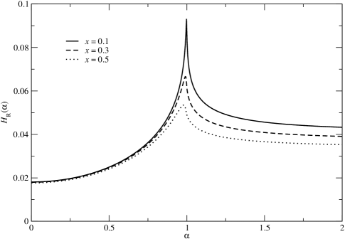
Figure 1: The function $H_{\mathrm{R}}(\alpha,x)$ vs $\alpha$ for different values of $x$.

IV.2 Pion dynamics

IV.2.1 Fluctuations around equilibrium

We begin our study by focusing on the real-time (quadratic) fluctuations around the equilibrium broken symmetry state for $T<T_{c}$, which is determined by the condition $d\mathcal{V}_{\mathrm{eff}}(\sigma_{0})/d\sigma_{0}=0$ with $\sigma_{0}\neq 0$. In this case, the real-time dynamics of pions is determined by the Laplace transform

$$\widetilde{\chi}(\mathbf{k},s)=\frac{1}{s}\left[1-\frac{H(0)}{(1+\xi^{2})H(i\xi,x)}\right]\chi(\mathbf{k},0).$$ (78)

After the analytic continuation $s\to i\omega+\epsilon$ and introducing the dimensionless variable $\alpha=\omega/k$, we find the real and imaginary parts of the analytically continued function $H(\alpha+i\epsilon)$ given by

$$H_{\mathrm{R}}(\alpha,x) = \frac{1}{4\pi^{2}}\int_{0}^{\bar{\Lambda}}\frac{dzz^{2}}{\epsilon^{2}}\bigg{[}\frac{\tanh\frac{\epsilon(z,x)}{2}}{\epsilon(z,x)}-\frac{1}{2\cosh^{2}\frac{\epsilon(z,x)}{2}}\bigg{(}1-\frac{\alpha\epsilon(z,x)}{2z}\ln\left|\frac{\alpha+z/\epsilon(z,x)}{\alpha-z/\epsilon(z,x)}\right|\bigg{)}\bigg{]},$$

$$H_{\mathrm{I}}(\alpha,x) = \frac{\alpha}{16\pi}\,\Theta(\alpha_{\mathrm{max}}^{2}-\alpha^{2})\int_{z_{\mathrm{min}}}^{\bar{\Lambda}}\frac{dzz}{\epsilon(z,x)\cosh^{2}\frac{\epsilon(z,x)}{2}},$$ (79)

respectively,

$$\alpha_{\mathrm{max}}=\bar{\Lambda}/\sqrt{\bar{\Lambda}^{2}+x^{2}}~{}~{};~{}~{}z_{\mathrm{min}}=x\alpha/\sqrt{1-\alpha^{2}}$$ (80)

The real part can be written in the following manner which separates the terms that are most sensitive to the cutoff

$$H_{\mathrm{R}}(\alpha,x) = \frac{1}{4\pi^{2}}\ln(\bar{\Lambda})+\frac{1}{4\pi^{2}}\int_{0}^{\bar{\Lambda}}\frac{dz}{z}\Bigg{[}\frac{\tanh\left(\frac{1}{2}\sqrt{x^{2}+z^{2}}\right)}{\left(1+\frac{x^{2}}{z^{2}}\right)^{3/2}}-\Theta(z-1)\Bigg{]}+B(\alpha,x)$$ (81)

$$B(\alpha,x) = -\frac{1}{4\pi^{2}}\int_{0}^{\bar{\Lambda}}\frac{dzz^{2}}{\epsilon^{2}}\frac{1}{2\cosh^{2}\frac{\epsilon(z,x)}{2}}\bigg{(}1-\frac{\alpha\epsilon(z,x)}{2z}\ln\left|\frac{\alpha+z/\epsilon(z,x)}{\alpha-z/\epsilon(z,x)}\right|\bigg{)}$$ (82)

The second term in eqn. (81) is rather insensitive to $\bar{\Lambda}$ and in this expression $\bar{\Lambda}$ can be taken to infinity with an exponentially small error. The form of $H(\alpha,x)$ above displays explicitly the dependence on $\bar{\Lambda}$.

The real and imaginary parts given in (79) are plotted in Figs. 1 and 2, respectively, for $N_{c}=3,N_{f}=2$, the values of $G,\Lambda$ given by eqn. (3) and different values of $x$ in the Landau-Ginzburg region $x\ll 1$.

The real part $H_{\mathrm{R}}(\alpha,x)$ increases monotonically for $0<\alpha\lesssim\alpha_{\mathrm{max}}$ then decreases monotonically to its asymptotic value for $\alpha\gg 1$. Furthermore, $H_{\mathrm{R}}(\alpha,x)$ features a sharp cusp near $\alpha\lesssim\alpha_{\mathrm{max}}$ as $x\to 0$. This cusp implies infrared divergence in the self-energies at the critical point $x=0$ and, as will be seen below, has a importance consequence on the relaxation of critical fluctuations. The imaginary part $H_{\mathrm{I}}(\alpha,x)$, which is completely determined by Landau damping only has support in the interval $-\alpha_{\mathrm{max}}<\alpha<\alpha_{\mathrm{max}}$.

The analytic properties of the quark loop diagram at finite temperature had also been studied in ref.caldas .

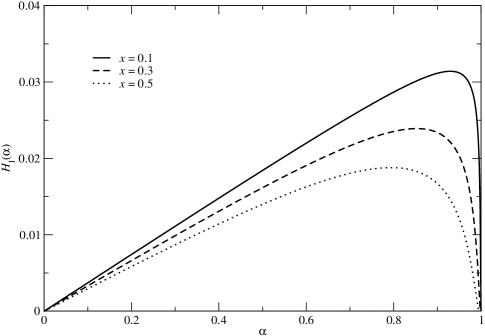
Figure 2: The function $H_{\mathrm{I}}(\alpha,x)$ vs $\alpha$ for different values of $x$.

The analytic continuation of the propagator to real frequency features the following singularities:

• Isolated poles. Isolated real poles describe stable quasiparticle excitations, whereas complex poles (on the second sheet) correspond to resonances with finite width. From (72) and (76), isolated poles of the Laplace transform for the pion field are determined by the equations:

  $$(1-\alpha^{2})H_{\mathrm{R}}(\alpha,x)=0,\quad(1-\alpha^{2})H_{\mathrm{I}}(\alpha,x)=0.$$ (83)

  Since $H_{\mathrm{I}}(\alpha,x)$ vanishes at $\alpha=\pm 1$, there are isolated real poles at $\alpha=\pm 1$ provided that $H_{\mathrm{R}}(\alpha,x)$ remains finite there. This indeed is the case below the critical point when $x>0$. Specifically, $H_{\mathrm{R}}(1)$ is a monotonically decreasing function for $x>0$ and its asymptotic behavior for $x\ll 1$ is found to be given by

  $$H_{\mathrm{R}}(1)\stackrel{{\scriptstyle x\ll 1}}{{\simeq}}-\frac{1}{4\pi^{2}}\Bigg{[}\ln\left(\frac{x}{\pi}\right)+\mathcal{O}(x^{0})\Bigg{]}.$$ (84)

  Thus for $x>0$ pions are sharp quasiparticles in this approximation that propagate with a dispersion relation $\omega_{\pi}(k)=\pm k$, namely with unit group velocity.

• Branch cuts. Branch cuts represent multiparticle states. In the long-wavelength, low-frequency limit there is only a branch cut on the real frequency axis in the region $-\alpha_{\mathrm{max}}k<\omega<\alpha_{\mathrm{max}}k$, corresponding to Landau damping processes in which the pion scatters off a quark in the medium.

Having identified the singularities of the Laplace transform $\widetilde{\chi}(\mathbf{k},s)$, we can perform the inverse Laplace transform (74) and obtain the real-time evolution

$$\frac{\chi(\mathbf{k},t)}{\chi(\mathbf{k},0)}=\int_{-\infty}^{\infty}\frac{d\alpha}{\alpha}\rho(\alpha)\cos\alpha\tau,$$ (85)

where $\tau=kt$, $\rho(\alpha)$ is the spectral function for the pion. In what follows we set $\chi(\mathbf{k},0)=1$ for notational simplicity. The spectral function $\rho(\alpha)$ receives contributions from the quasiparticle poles and the Landau damping cut:

$$\rho(\alpha)=Z\,\mathrm{sgn}(\alpha)\,\delta(1-\alpha^{2})+\rho_{\mathrm{cut}}(\alpha),$$ (86)

where $\mathrm{sgn}(\alpha)$ is the sign function, $Z$ is the residue of the pion poles at $\alpha=\pm 1$, and $\rho_{\mathrm{cut}}(\alpha)$ denotes the cut contribution

$$Z=\frac{H_{\mathrm{R}}(0,x)}{H_{\mathrm{R}}(1,x)},\quad\rho_{\mathrm{cut}}(\alpha)=\frac{H_{\mathrm{R}}(0,x)H_{\mathrm{I}}(\alpha,x)}{\pi(1-\alpha^{2})[H_{\mathrm{R}}^{2}(\alpha,x)+H_{\mathrm{I}}^{2}(\alpha,x)]}.$$ (87)

Therefore the real-time solution is given by

$$\chi(\mathbf{k},t)=\chi_{\mathrm{pole}}(\mathbf{k},t)+\chi_{\mathrm{cut}}(\mathbf{k},t),$$ (88)

where for $\chi(\mathbf{k},0)=1$, we find

$$\chi_{\mathrm{pole}}(\mathbf{k},t)=Z\cos\tau,$$

$$\chi_{\mathrm{cut}}(\mathbf{k},t)=2\int_{0}^{\alpha_{\mathrm{max}}}\frac{d\alpha}{\alpha}\rho_{\mathrm{cut}}(\alpha)\cos\alpha\tau,\quad\tau=kt.$$ (89)

Setting $t=0$ in (89) [with $\chi(\mathbf{k},0)=1$], we obtain the following sum rule for the spectral function

$$Z+2\int_{0}^{\alpha_{\mathrm{max}}}\frac{d\alpha}{\alpha}\rho_{\mathrm{cut}}(\alpha)=1,$$ (90)

which we have verified numerically for a wide range of $x$.

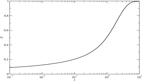
Figure 3: The residue of the pion pole $Z$ vs $x$.

The quasiparticle poles give rise to an undamped oscillation with an amplitude determined by the residue $Z$. Figure 3 displays the residue of the quasiparticle pole $Z$ as a function of $x$. It shows clearly that away from the GL region in the low-temperature limit ($x\gg 1$) the spectral function is dominated by the isolated pion pole since $Z\approx 1$. Thus Landau damping is negligible and pions are stable excitations. This is because Landau damping is solely a medium effect arising from scatterings of pions with quarks in the heat bath, hence its contribution at lower temperature is less important. In the GL region ($x\ll 1$) the continuum contribution from the Landau damping cut dominates the spectral function, since in this region $Z\ll 1$. Figure 3 also shows a crossover at $x\sim 1$ at which $Z\sim 1/2$, hence the isolated pole and the continuum contributions are of equal importance. The Landau damping contribution to the spectral function $\rho_{\mathrm{cut}}(\alpha)$ is displayed in Fig. 4. For $x\ll 1$, it reveals clearly a sharp peak near the threshold, indicating the emergence of an infrared divergence at the critical point.

Equation (84) and the fact that $H_{\mathrm{R}}(0)$ is finite and non-vanishing at $x=0$ entail that near the critical temperature, namely $x\ll 1$, the residue of the pion pole behaves as

$$Z\propto\frac{1}{\left|\ln\frac{T_{c}-T}{T_{c}}\right|}.$$ (91)

where we have used that $x=m(T)/T$ and $m(T)=G\sigma_{eq}(T)\propto(T_{c}-T)^{1/2}$ by eqn. (60).

Therefore the residue at the isolated pion pole vanishes as $T\rightarrow T_{c}$ from below. As the critical point is approached, the weight of the isolated pole to the spectral function becomes negligible and exactly at the critical point the residue vanishes and the isolated pole merges with the continuum contribution. Thus it is clear that as the critical region is approached, the edge of the Landau damping cut begins to dominate the spectral function.

The Landau damping contribution to the real-time evolution of a long-wavelength pion fluctuation $\chi_{\mathrm{cut}}(\mathbf{k},\tau)$ is plotted in Fig. 5. The value at $\tau=0$ equals $1-Z$ by the sum rule, thus it is clear from this figure that for small $x$, namely $T\lesssim T_{c}$, the continuum contribution dominates over that of the isolated pole. This figure also reveals several time scales: a rapid damping as a function of the scaled variable $\tau=kt$ towards an oscillating amplitude, which is of the same order as the isolated pole contribution $Z\ll 1$ and oscillates with a frequency $\alpha\simeq 1$ and slowly damped out on longer time scale . The frequency of these oscillations is clearly determined by the sharp rise of the Landau damping contribution near $\alpha=1$.

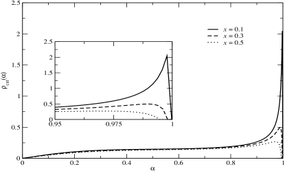
Figure 4: The cut contribution to the spectral function $\rho_{\mathrm{cut}}(\alpha)$ vs $\alpha$ for different values of $x$. The inset shows the behavior of $\rho_{\mathrm{cut}}(\alpha)$ near the threshold $\alpha=\alpha_{\mathrm{max}}$.

Although for $T<T_{c}$ the pion is a stable quasiparticle, its oscillating amplitude $Z$ vanishes as the critical temperature is approached thus near the critical point the initial amplitude is completely damped out by Landau damping. As $T\to T_{c}$ from below the amplitude of long-wavelength pion fluctuations is damped by Landau damping on a scale $\tau_{*}$ which is numerically insensitive to $x$ for $x\lesssim 0.2$ and is approximately $\tau_{*}\sim 5$ for the values of coupling and cutoff given by eq. (3). In terms of the physical time, we see that the amplitude of long-wavelength pion fluctuations relaxes on a time scale $t_{\mathrm{rel}}(k)=\tau_{*}/k$, where $\tau_{*}\sim 5$ is numerically found to be rather insensitive to $x$. Thus relaxation of long-wavelength pion fluctuations near the critical point are critically slow.

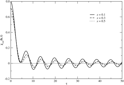
Figure 5: $\chi_{\mathrm{cut}}(\mathbf{k},\tau)$ vs $\tau$ in the GL region.

IV.2.2 Dynamics at the critical point

As remarked above, the self-energies feature a logarithmic threshold divergence at the critical point. Indeed, for $x\to 0$ the real and imaginary parts of $H(\alpha+i\epsilon)$ can be approximated, respectively, as

$$H_{\mathrm{R}}(\alpha,x) \stackrel{{\scriptstyle x\to 0}}{{\simeq}} \frac{1}{4\pi^{2}}\bigg{[}\int_{0}^{\bar{\Lambda}}\frac{dz}{z}\tanh\frac{z}{2}-\bigg{(}1-\frac{\alpha}{2}\ln\left|\frac{\alpha+1}{\alpha-1}\right|\bigg{)}\tanh\frac{\bar{\Lambda}}{2}\bigg{]},$$

$$H_{\mathrm{I}}(\alpha,x) \stackrel{{\scriptstyle x\to 0}}{{\simeq}} \frac{\alpha}{8\pi}\,\Theta(1-\alpha^{2})\tanh\frac{\bar{\Lambda}}{2}.$$ (92)

Whereas the analytically continued inverse pion propagator vanishes as $\alpha^{2}\to 1$ (with a logarithmic divergent slope for the real part), the values $\alpha=\pm 1$ ($\omega=\pm k$) are longer identified with quasiparticle poles but the endpoints of the logarithmic branch cut. This threshold singularity is reminiscent to those in QED and in equilibrium critical phenomenaboyan . In the former case the self-energy of a charged particle has a logarithmic infrared divergence near the threshold arising from the emission of soft gauge bosons. In the latter case logarithmic infrared divergences appear in correlation functions near the critical point at the upper critical dimension. The emergence of infrared divergences in both cases indicates the breakdown of perturbation theory and calls for a nonperturbative resummation of the infrared divergencesboyan .

To display the logarithmic threshold divergence in an explicit manner, let us focus on the Laplace transform of the inverse pion propagator [see (76)], which near the threshold at the critical point can be approximated as

$$D_{\pi}^{-1}(k,s) = g\,\mathcal{C}\,\bar{k}^{2}(1+\xi^{2})\left[1+i\xi\lambda\ln\frac{i\xi+1}{i\xi-1}\right]$$ (93)

$$\stackrel{{\scriptstyle\xi^{2}\to-1}}{{\simeq}} g\,\mathcal{C}\,\bar{k}^{2}(1+\xi^{2})\left\{1-\lambda\ln[-(1+\xi^{2})]+\cdots\right\},$$

where

$$\mathcal{C}=H_{\mathrm{R}}(0),\quad\lambda=\frac{1}{8\pi^{2}\mathcal{C}}\tanh\frac{\bar{\Lambda}}{2}\approx 0.683,$$ (94)

and the dots denotes terms that are formally of order $\lambda$ but remain finite in the limit $\xi^{2}\to-1$. Such logarithmic threshold divergence at the critical point is akin to that found in Ref. boyan . In this reference a finite-temperature version of the renormalization group was introduced to provide a resummation of these threshold divergences which leads to an exponentiation and anomalous dimensions near threshold.

The logarithmic threshold divergence featured by the pion propagator (93) suggests the buildup of an anomalous dimension. The results of Ref. boyan would suggest that the leading logarithmic enhancement of the pion self-energy at threshold eq. (93) could exponentiate leading to a resummed inverse pion propagator near the pion mass shell

$$D_{\pi}^{-1}(k,s)\simeq-g\,\mathcal{C}\,\bar{k}^{2}\left[-(1+\xi^{2})\right]^{1-\lambda}\quad\mbox{for}\quad\xi^{2}\to-1,$$ (95)

which, after analytic continuation $i\xi\to\alpha+i\epsilon$, gives

$$D_{\pi}^{-1}(k,\omega) \simeq -g\,\mathcal{C}\,\bar{k}^{2}\,|1-\alpha^{2}|^{1-\lambda}\big{\{}\cos[\lambda\pi\Theta(1-\alpha^{2})]$$ (96)

$$+i\,\mbox{sgn}(\alpha)\,\sin\lambda\pi\,\Theta(1-\alpha^{2})\big{\}}\quad\mbox{for}\quad\alpha^{2}\to 1.$$

Such an exponentiation if correct would reveal a new dynamical exponent (anomalous dimension) $\lambda$, which however is numerically large to be justified by a perturbative approach.

Obviously at this stage we can only speculate that such an exponentiation actually emerges based on the study of Ref. boyan . A full analysis of whether a finite-temperature renormalization group approach can be systematically implemented in this theory, remains at this stage an open question that deserves further study and which is clearly beyond the scope of this article.

IV.2.3 Non-locality of the real-time effective action

An important aspect of the pion self-energy is that it is non-analytic for fixed $k$ as $\omega\rightarrow 0$. In particular this non-analyticity of the function $H(\alpha)$ entails that the limits $k\rightarrow 0$ and $\omega\rightarrow 0$ do not commute. Furthermore, this branch cut prevents a well-defined expansion in powers of $k$ or $\omega$, which in turn translates in that the effective action is non-local in space and time and cannot be expressed as a gradient expansion in terms of space and time derivatives of the fields. This non-locality is similar to that in the hard thermal loop effective action in gauge theories brapis ; lebellac which also originates in Landau damping.

To highlight this point more clearly, we focus on the limits $k,\,\omega\rightarrow 0$ of the retarded inverse pion propagator [see eqs. (76)]

$$D^{-1}_{\mathrm{ret}}(k,\omega)=\widetilde{D}^{-1}_{\pi}(k,s=i\omega+\epsilon)=-(\omega^{2}-k^{2})\left[H_{\mathrm{R}}(\alpha,x)+iH_{\mathrm{I}}(\alpha,x)\right].$$ (97)

We find the following limits

$$D^{-1}_{\mathrm{ret}}(k,0)=k^{2}H_{\mathrm{R}}(0),\quad D^{-1}_{\mathrm{ret}}(0,\omega)=-\omega^{2}H_{\mathrm{R}}(\infty),$$ (98)

with $H_{\mathrm{R}}(0)$ and $H_{\mathrm{R}}(\infty)$ slowly varying functions of the temperature near $T_{c}$. Their values at $T=T_{c}$ are given by

$$H_{\mathrm{R}}(0,T=T_{c})=0.015,\quad H_{\mathrm{R}}(\infty,T=T_{c})=0.04.$$ (99)

The limits (98) would seem to suggest that there are stable long-wavelength pion fluctuations that propagate with a dispersion relation

$$\omega^{2}=v^{2}k^{2},\quad v^{2}=\frac{H_{\mathrm{R}}(0)}{H_{\mathrm{R}}(\infty)}\approx 0.375.$$ (100)

However, such conclusion is obviously incorrect, for $T<T_{c}$ there are stable, long-wavelength pion fluctuations that propagate with unit group velocity since the isolated pion poles correspond to $\alpha^{2}=1$ [see eq. (83)]. Landau damping thus prevents a local description of the low-energy effective action as an expansion in spatiotemporal gradients. This point will be important below when we discuss our results in light of previous studies.

IV.3 Away from equilibrium: spinodal instabilities

During a rapid phase transition, early stages of the nonequilibrium dynamics is dominated by spinodal instabilities, i.e., long-wavelength fluctuations are unstable and their amplitude grows exponentially during the early stages spino . These instabilities result in the emergence of correlated domains, which in the case under consideration are coherent domains of pions which have been identified as disoriented chiral condensates DCC . Spinodal instabilities emerge when the order parameter is not at the minimum of the free energy for $T<T_{c}$ but is still “rolling” towards it.

In the case under consideration the equilibrium minimum in the GL region is determined by eq. (60). Hence below the critical temperature and in the GL region, we have

$$\frac{1}{\sigma_{0}}\frac{d\mathcal{V}_{\mathrm{eff}}(\sigma_{0})}{d\sigma_{0}}=b\left[\sigma^{2}_{0}-\sigma^{2}_{\mathrm{eq}}(T)\right]\equiv-\Delta^{2}(T),$$ (101)

with $\Delta^{2}(T)>0$ in the spinodal region $|\sigma_{0}|<\sigma_{\mathrm{eq}}(T)$. The inverse pion propagator (76) in the GL region away from equilibrium can now be written as

$$\widetilde{D}^{-1}_{\pi}(k,s)=g(\bar{s}^{2}+\bar{k}^{2})H(i\xi,x)-\Delta^{2}(T),$$ (102)

where we have restored the term in (101) which is absent in equilibrium. It is clear from the inverse Laplace transform expression that yields the real-time evolution (74) that real poles in the Laplace variable $s$ correspond to exponentially growing (or decaying) solutions. If the real part of the pole is positive, the real-time evolution describes an instability with a consequent exponential growth of small amplitude fluctuations.

For spatially homogeneous pion fluctuations ($k=0$) in the spinodal region of the phase diagram with $|\sigma_{0}|<\sigma_{\mathrm{eq}}(T)$ for which $\Delta^{2}(T)>0$, the inverse pion propagator becomes

$$\widetilde{D}^{-1}_{\pi}(0,s)=g\,s^{2}I(T)-\Delta^{2}(T),$$ (103)

where

$$I(T)=\frac{1}{4\pi^{2}}\int_{0}^{\bar{\Lambda}}\frac{dzz^{2}}{\epsilon^{3}}\tanh\frac{\epsilon}{2}~{}~{};~{}~{}I(T_{c})=\frac{1}{4\pi^{2}}\,\ln\left(\frac{2~{}\bar{\Lambda}~{}e^{\gamma}}{\pi}\right).$$ (104)

with $\gamma$ the Euler-Mascheroni constant. The pion propagator has real poles at

$$s^{2}_{*}=\frac{\Delta^{2}(T)}{g\,I(T)},$$ (105)

which describes one growing and one decaying solution. The growing solution has growth rate given by (for $T<T_{c}$)

$$\Gamma_{*}(k=0,T)=\frac{\Delta(T)}{\sqrt{g\,I(T)}}\propto\big{[}\sigma^{2}_{\mathrm{eq}}(T)-\sigma^{2}_{0}\big{]}^{\frac{1}{2}}.$$ (106)

The classical spinodal corresponds to the region of order parameter in the phase diagram for which the system is thermodynamically unstable to long-wavelength perturbations spino . This corresponds to the values of the order parameter for which the zero momentum growth rate $\Gamma_{*}(k=0,T)\neq 0$. Therefore we see that the classical spinodal line corresponds to $|\sigma_{0}|<\sigma_{\mathrm{eq}}(T)$. This is the same as the classical spinodal in the mean field approximation for the GL effective theory or the linear sigma model. This can be seen from the Lagrangian density (II). Since along the classical spinodal $(1/\sigma_{0})~{}dV(\sigma_{0})/d\sigma_{0}<0$, hence the mass squared term for the pions is negative and small amplitude pion fluctuations are unstable and grow exponentially spino .

While obtaining the growth rate for arbitrary $k$ is an involved numerical task which is not very illuminating, we can learn much by obtaining $\Gamma_{*}(k,T)$ in the long-wavelength limit $k^{2}/\Delta^{2}(T)\ll 1$. This is achieved by expanding the function $H(is/k)$ for large values of the ratio $s/k$ and solving for the position of the (real) pole in the variable $s$. This expansion is valid since the function $H$ is analytic everywhere away from the Landau damping cut along the imaginary axis in the complex $s$-plane. After straightforward algebra we find

$$\Gamma_{*}(k,T)=\left[\frac{\Delta^{2}(T)}{g\,I(T)}-[1-J(T)]\,k^{2}+g\,I(T)\,J(T)\frac{k^{4}}{\Delta^{2}(T)}+\mathcal{O}\left(\frac{k^{6}}{\Delta^{4}(T)}\right)\right]^{\frac{1}{2}},$$ (107)

where

$$J(T)=\frac{1}{24\pi^{2}}\int_{0}^{\bar{\Lambda}}\frac{dzz^{4}}{\epsilon^{4}}\frac{1}{\cosh^{2}\frac{\epsilon}{2}}~{}~{};~{}~{}J(T_{c})=\frac{1}{12\pi^{2}}.$$ (108)

While the expression (107) can be expanded in a power series in $k^{2}$ in the long-wavelength limit, we have purposely kept the powers of $k$ inside the square root to compare with the growth rate predicted by the linear sigma model (II)

$$\Gamma_{\mathrm{LSM}}(k,T)=\left[\left|\frac{1}{\sigma_{0}}\frac{dV(\sigma_{0})}{d\sigma_{0}}\right|-k^{2}\right]^{\frac{1}{2}}.$$ (109)

The corrections to the coefficient of $k^{2}$ as well as the higher powers of $k$ in the growth rate (107) all originate in the non-local Landau damping contribution.

V Conclusions and summary of main results

In this article we have studied the low-energy effective action for meson fields in the two-flavor NJL constituent quark model. The main goal and focus are to study static and dynamical phenomena near the critical point for the chiral phase transition and explore whether the low-energy effective action describes the same universality class as the O(4) linear sigma model wilraja or the nonlinear sigma model son .

We have obtained the low-energy effective action by integrating out the quark fields to lowest order in the loop expansion up to quadratic order in the fluctuations around a mean field configuration. In this constituent quark model, the meson degrees of freedom emerge as scalar and pseudoscalar bound states of quark and antiquarks and their space-time dynamics is completely determined by the underlying quark model. Both the static as well as the dynamical aspects where studied in the low-energy, long-wavelength limit and in the GL region near the critical point in the broken symmetry phase. The evaluation of the effective potential (free energy for a mean field configuration) as well as the self-energies for the scalar and pseudoscalar mesons allow us to obtain the effective action from which we can extract the static limit. The scalar and pseudoscalar self-energies are obtained to lowest order in the loop expansion upon integrating out the quark degrees of freedom. The imaginary parts of the self-energies in the low-energy, long-wavelength limits are completely determined by Landau damping resulting from quark (antiquark) scattering in the medium. The integration of the quark degrees of freedom in the real-time effective action allows us to obtain the equations of motion for scalar and pseudoscalar (pion) meson fluctuations around the mean field and to study the real-time evolution of small amplitude fluctuations as an initial value problem. The study of the real-time dynamics near the critical point allows us to explore dynamical critical phenomena.

Our conclusions and main results are the following:

• Static critical phenomena. We have established that the low-energy effective action in the static limit up to quadratic order in the fluctuations around the mean field, which is obtained by integrating out the quark fields up to one loop, coincides with the GL free energy including the spatial gradients in the long-wavelength limit. Thus the static limit of the NJL constituent quark model with two flavors is in the same universality class as the O(4) linear sigma model (Heisenberg ferromagnet) in agreement with the conjecture in Ref. wilraja .

• Dynamical critical phenomena. Dynamical phenomena of pions near the critical point is studied by focusing on the equations of motion for small amplitude pseudoscalar fluctuations around a mean field configuration. The equations of motion are solved by Laplace transform as an initial value problem. For fluctuations around the equilibrium minimum of the effective potential below the critical temperature, we find that there are stable long-wavelength pion excitations corresponding to poles away from the continuum in the pion propagators. The dispersion relation of the stable pion excitations is $\omega_{\pi}(k)=k$ and the residue at the pion pole vanishes as $Z\propto 1/|\ln(1-T/T_{c})|$ as $T\rightarrow T_{c}$ from below. The amplitude of the pion fluctuations is Landau damped on a time scale $t_{\mathrm{rel}}(k)=\tau_{*}/k$ with $\tau_{*}$ a slowly varying function of temperature near $T_{c}$. Thus near the critical temperature relaxation of long-wavelength pion fluctuations are critically slow. At the critical temperature, the isolated pion pole merges with the Landau damping continuum resulting in a logarithmic divergence on the pion mass shell similar to the logarithmic enhancement found in Ref. boyan . Based on the renormalization group arguments of Ref. boyan we conjecture that such a logarithmic divergence on the pion mass shell at the critical temperature is the harbinger of a dynamical anomalous dimension $\lambda$, which however turns out to be fairly large in this model, $\lambda\sim 0.683$.

  We have studied the dynamics of fluctuations away from the equilibrium minima of the effective potential to assess the growth rate of spinodal fluctuations. We find that the classical spinodal line coincides with that of the mean field description of the GL linear sigma model. However, the growth rate for long-wavelength spinodal fluctuations is different from those obtained from the GL effective theory. The Landau damping contribution to the self-energy leads to a richer wavelength dependence of the growth rate of small amplitude spinodal fluctuations.

Thus we conclude that whereas static critical phenomena is described by the universality class of the O(4) Heisenberg ferromagnet (linear sigma model) near the critical temperature, dynamical critical phenomena is not in the same universality class. We also conclude that below the critical temperature there are stable pion excitations with a dispersion relation $\omega_{\pi}(k)=k$, namely with unit group velocity. This result is in disagreement with those found in Ref. son . We argue that the source of disagreement is likely to be found in the derivative expansion of the effective action as proposed in Ref. son . We argue that such derivative expansion leading to a local effective action is not reliable because the Landau damping contribution to the pion self-energy introduces a cut in the complex frequency plane along the real axis, which at the critical point is in the region $-k<\omega<k$. This cut results in that the real-time effective action is non-local and cannot be expanded in spatio-temporal derivatives. The results of our one loop calculation must be compared with the results of the one-loop calculation in the linear sigma model in the first article of ref.son where the limits $\vec{k}\rightarrow 0,\omega=0$ and the limit $\omega\rightarrow 0,\vec{k}=\vec{0}$ are studied. The Landau damping cut for $-k\leq\omega\leq k$ where the pion propagator is non-analytic makes these two limits not commutative. We suspect that this non-analyticity is at the heart of the discrepancy between our results and those of ref.son , at least at the one-loop level which is common to both studies.

Such a non-analytic structure below the light cone is akin to that found in the hard thermal loop limit of gauge theories which also arises precisely from Landau damping brapis ; lebellac . At the critical point we find a logarithmic divergence on the pion mass shell, again originating in the Landau damping processes. These logarithmic divergences are akin to those found in Ref. boyan and suggest the buildup of (in this case a large) dynamical anomalous dimension.

Caveats: beyond lowest order. Our results are based on integrating out the quark degrees of freedom at lowest order in the loop expansion. Given that the effective coupling is not small the validity of such an expansion can be called into question. Such expansion becomes exact in the large-$N_{f}N_{c}$ limit, however, taking $N_{f}N_{c}$ to be large for fixed coupling $G^{2}$ one can see from eq. (23) that $T_{c}\approx\Lambda$ and the regime of validity of the constituent quark model as a description of the critical properties must be re-assessed. In the linear (or nonlinear) sigma model effective field theory, the self-energy corrections arise from interaction terms between scalar and pseudoscalar fluctuations. For example some of the results of Ref. son are based on a one-loop contribution to the pion self-energy from the $\delta$-$\pi$-$\pi$ vertex below $T_{c}$. One could obtain the effective $\delta$-$\pi$-$\pi$ vertex from the constituent quark model also in one-loop approximation by going beyond quadratic order in the fluctuations. Such vertex necessarily must be proportional to $m$ by chiral symmetry. A local limit of such vertex can be obtained by taking first the static and then the long-wavelength limit. However, using such local vertex to calculate real-time dynamics would not be consistent and the non-local form factor of the vertex must be taken into account to calculate the corrections to the pion self-energies. Such calculation is clearly much more complicated than that in the local effective field theory because of the momentum and frequency dependence of the vertex are likely to change the results of Refs. son ; boyan .

At the order considered, below the critical temperature the pion pole is isolated, this is a consequence that to this leading order there are no scattering contributions and therefore the pion does not acquire a collisional width. Of course this situation will change beyond this order, in particular corrections to next to leading order in the large $N_{c}N_{f}$ limit will lead to scattering corrections and the pion will acquire a collisional width, whose behavior near the critical point must be studied. The collisional width of the pion is an important ingredient in the manifestation of the axial anomaly at finite temperatureanomaly whose understanding thus requires to go beyond one-loop order, which is the leading order in the large $N_{c}N_{f}$ limit. Furthermore, as we mentioned in the introduction, a well known shortcoming of the NJL model is its lack of confinementhatsuda ; klevansky , which is manifest in that free quarks are present in the thermal bath below the critical temperature for chiral symmetry. Clearly there are no models, short of full QCD that can overcome this problem.

The logarithmic threshold enhancement near the critical point suggests that a resummation scheme such as a renormalization group program as proposed in ref.boyan must be implemented to approach the critical region in a reliable manner.

The study of the long-wavelength small frequency limit requires a resummation of self-energy and vertex diagrams, just like in the case of transport phenomenajeon ; conductivity as a consequence of the emergence of “pinch singularities”jeon which are manifest as secular terms in the perturbative expansion in real timeconductivity . In ref.conductivity it was shown that such resummation can be implemented via a dynamical renormalization group. It is clearly interesting and important to study the long-wavelength and small frequency limit near the critical point implementing these resummation schemes, perhaps supplemented by a renormalization of the scattering amplitudes near the critical point as suggested in ref.boyan . Clearly such program is well beyond the one loop approximation which despite the fact of being the leading order in the large $N_{c}N_{f}$ limit, does not include self-energy and vertex corrections which are necessary for a full resummation programjeon ; conductivity .

The implementation of such program is beyond the scope of this study.

Thus our study suggests that the static critical phenomena is well described by a GL low-energy effective theory, but that the dynamical aspects are richer, with novel dynamical critical phenomena whose universality must be studied in detail. Our study at the one-loop level should be taken as indicative of novel dynamical phenomena emerging near the critical point and calls for resummation program perhaps by implementing a renormalization group approach akin to that of Ref. boyan but directly in the constituent quark model for a deeper understanding of dynamical scaling and anomalous dimensions.

- (1) R.D. Pisarski and F. Wilczek, Phys. Rev. D 29, 338 (1984); F. Wilczek, Int. J. Mod. Phys. A 7, 3911 (1992).
- (2) K. Rajagopal and F. Wilczek, Nucl.Phys. B399, 395 (1993); Nucl. Phys. B404, 577 (1993); K. Rajagopal, in Quark-Gluon Plasma 2, edited by R.C. Hwa (World Scientific, Singapore, 1995).
- (3) For recent reviews, see F. Karsch, Nucl. Phys. A698, 199 (2002); and references therein.
- (4) H. Meyer-Ortmanns, Rev. Mod. Phys. 68, 473 (1996); B. Müller, The Physics of the Quark-Gluon Plasma, Lecture Notes in Physics Vol. 225 (Springer-Verlag, Berlin, 1985); L.P. Csernai, Introduction to Relativistic Heavy Ion Collisions (John Wiley and Sons, Chichester, England, 1994); C.Y. Wong, Introduction to High-Energy Heavy Ion Collisions (World Scientific, Singapore, 1994).
- (5) M. Gell-Mann and M. Levy, Nuovo Cimento 16, 705 (1960).
- (6) D.J. Gross and A. Neveu, Phys. Rev. D 10, 3235 (1974).
- (7) Y. Nambu and G. Jona-Lasinio, Phys. Rev. 122, 345 (1961); 124, 246 (1961).
- (8) T. Hatsuda and T. Kunihiro, Phys. Rep. 247, 241 (1994), Phys. Rev. Lett. 55, 158 (1985), Phys. Lett. B 185, 304 (1987), Phys. Lett. B 198, 126 (1987); S. Chiku and T. Hatsuda Phys. Rev. D 57, 6 (1998); T. Hatsuda, T. Kunihiro and H. Shimizu Phys. Rev. Lett. 82, 2840 (1999).
- (9) S. Klevansky, Rev. Mod. Phys. 64, 649 (1992).
- (10) T.M. Schwarz, S.P. Klevansky, and G. Papp, Phys. Rev. C 60, 055205 (1999); O. Scavenius, A. Mocsy, I.N. Mishustin, and D.H. Rischke, 64, 045202 (2001).
- (11) A. Chodos, F. Cooper, W. Mao, H. Minakata, and A. Singh, Phys. Rev. D 61, 045011 (2000).
- (12) Z. Fodor and S. D. Katz, JHEP 203, 14 (2002); Nucl.Phys.Proc.Suppl. 106 441 (2002); Heavy Ion Phys. 18 41 (2003); hep-lat/0402006 ; hep-lat/0401023 ; Z. Fodor, Nucl.Phys. A715, 319 (2003); F. Csikor, G.I. Egri, Z. Fodor, S.D. Katz, K.K. Szabo, A.I. Toth, hep-lat/0401022; hep-lat/0401016, and references therein.
- (13) E. Laermann and O. Philipsen, hep-ph/0303042; O. Philipsen, hep-ph/0110051.
- (14) Ph. de Forcrand and O. Philipsen Nucl.Phys. B673 170 (2003); hep-lat/0309109; hep-ph/0301209.
- (15) C.R. Allton, S. Ejiri, S.J. Hands, O. Kaczmarek, F. Karsch, E. Laermann, Ch. Schmidt, L. Scorzato; Phys.Rev. D66 074507 (2002).
- (16) K. Rajagopal and F. Wilczek, Nucl. Phys. B399, 395 (1993); S. Gavin, A. Gocksch and R.D. Pisarski, Phys. Rev. Lett. 72, 2143 (1994); D. Boyanovsky, H.J. de Vega, and R. Holman, Phys. Rev. D 51 , 734 (1995); D. Boyanovsky, M. D’Attanasio, H.J. de Vega, and R. Holman, 54, 1748 (1996); F. Cooper, Y. Kluger, E. Mottola, and J.P. Paz, Phys. Rev. D 51, 2377 (1995); F. Cooper, Y. Kluger, and E. Mottola, Phys. Rev. C 54 3298, (1996); Y. Kluger, F. Cooper, E. Mottola, J.P. Paz, and A. Kovner, Nucl. Phys. A590, 581c (1995); J. Randrup, Phys. Rev. C 62, 064905 (2000); Nucl. Phys. A616, 531 (1997).
- (17) K. Rajagopal, Nucl. Phys. A680, 211 (2000); B. Berdnikov and K. Rajagopal, Phys. Rev. D 61, 105017 (2000); M. Stephanov, K. Rajagopal and E. Shuryak, Phys. Rev. D 60, 114028 (1999); J. Randrup, Phys. Rev. D 63, 061901 (2001), Heavy Ion Phys. 9, 289 (1999).
- (18) D. Boyanovsky, H.J. de Vega, R. Holman, and S.P. Kumar, Phys. Rev. D 56, 3929 (1997); Phys. Rev. D 56, 5233 (1997).
- (19) A. Chodos, F. Cooper, W. Mao, and A. Singh, Phys. Rev. D 63, 096010 (2001); F. Cooper and V.M. Savage, Phys. Lett. B 545, 307 (2002).
- (20) T. Koide and M. Maruyama, nucl-th/0308025.
- (21) D. Boyanovsky, H.J. de Vega, and M. Simionato, Phys. Rev. D 63, 045007 (2001); D. Boyanovsky, H.J. de Vega, 65, 085038 (2002); D. Boyanovsky and H.J. de Vega, Ann. Phys. (N.Y.) 307, 335 (2003); D. Boyanovsky, H. J. de Vega, R. Holman, M. Simionato , Phys.Rev. D60, 065003 (1999).
- (22) D.T. Son and M.A. Stephanov, Phys. Rev. D 66, 076011 (2002); Phys. Rev. Lett. 88, 202302 (2002).
- (23) In our definition of the NJL model given in eq. (1) the four-Fermi coupling is instead of the definition in Refs. hatsuda ; klevansky and we consider massless quarks.
- (24) J.I. Kapusta, Finite-Temperature Field Theory (Cambridge University Press, Cambridge, England, 1989).
- (25) D. Boyanovsky, D.-S. Lee, and A. Singh, Phys. Rev. D 48, 800 (1993); D. Boyanovsky, Phys. Rev. E 48, 767 (1993); D. Boyanovsky, H.J. de Vega, and R. Holman in Topological Defects and the Non-Equilibrium Dynamics of Symmetry Breaking Phase Transitions, edited by Y.M. Bunkov and H. Godfrin (Nato Science Series, Kluwer, 2000) [hep-ph/9903534]; and references therein.
- (26) M. Le Bellac, Thermal Field Theory (Cambridge University Press, Cambridge, England, 1996).
- (27) J. Schwinger, J. Math. Phys. 2, 407 (1961); L.V. Keldysh, Sov. Phys. JETP 20, 1018 (1965); K.T. Mahanthappa, J. Math. Phys. 47, 1 (1963); 47, 12 (1963); K.-C. Chou, Z.-B. Su, B.-L. Hao, and L. Yu, Phys. Rep. 118, 1 (1985).
- (28) See, for example, D. Boyanovsky, H.J. de Vega, R. Holman, and D.-S. Lee, Phys. Rev. D 52, 6805 (1995); D. Boyanovsky, M. D’Attanasio, H.J. de Vega, and R. Holman, 54, 1748 (1996); and references therein.
- (29) D. Boyanovsky, H.J. de Vega, D.-S. Lee, Y.J. Ng, and S.-Y. Wang, Phys. Rev. D 59, 105001 (1999); S.-Y. Wang, D. Boyanovsky, H.J. de Vega, D.-S. Lee, and Y.J. Ng, Phys. Rev. D 61, 065004 (2000); S.-Y. Wang, D. Boyanovsky, H.J. de Vega, and D.-S. Lee, Phys. Rev. D 62, 105026 (2000); and references therein.
- (30) H.C. de Godoy Caldas and M. Hott, Phys.Rev. D67 045011 (2003); H.C.G. Caldas, A.L. Mota, M.C. Nemes, Phys.Rev. D63 056011 (2001); H.C. de Godoy Caldas, Nucl.Phys. B623 503 (2002).
- (31) E. Braaten and R.D. Pisarski, Nucl. Phys. B337, 569 (1990); B339, 310 (1990); R.D. Pisarski, Physica A 158, 146 (1989); Phys. Rev. Lett. 63, 1129 (1989); Nucl. Phys. A525, 175 (1991).
- (32) H.Itoyama and A. H. Mueller, Nucl. Phys. B218, 349 (1983); S. P. Kumar, D. Boyanovsky, H. J. de Vega, R. Holman, Phys. Rev. D61 065002 (2000).
- (33) S. Jeon, Phys. Rev. D52, 3591 (1995); S. Jeon and L.G. Yaffe, Phys. Rev. D53, 5799 (1996).
- (34) D. Boyanovsky, H. J. de Vega and S.-Y. Wang, Phys. Rev. D67, 065022 (2003).