1 Introduction

There is increasing experimental evidence [1, 2] for the existence of a narrow baryon resonance $\Theta^{+}$ with strangeness $S=+1$, whose minimal quark content is $uudd\bar{s}$. Triggered by the prediction of its mass and width in [3], the observation of this hadron promises to shed new light on our picture of baryons in QCD, with theoretical approaches as different as the soliton picture [3, 4], quark models [5], and lattice calculations [6], to cite only a fraction of the literature. A fundamental question is how the structure of baryons manifests itself in terms of the basic degrees of freedom in QCD, at the level of partons. This structure at short distances can be probed in hard exclusive scattering processes, where it is encoded in generalized parton distributions [7] (see [8, 9] for recent reviews). In this letter we introduce the transition GPDs from the nucleon to the $\Theta^{+}$ and investigate electroproduction processes where they could be measured, hopefully already in existing experiments at DESY and Jefferson Lab.

In the next section we give some basics of the processes we propose to study. We then define the generalized parton distributions for the $N\to\Theta$ transition and discuss their physics content (throughout this paper we write $N$ for the nucleon and $\Theta$ for the $\Theta^{+}$). The scattering amplitudes and cross sections for different production channels are given in Section 4. In Section 5 we evaluate the contribution from kaon exchange in the $t$-channel to the processes under study. Concluding remarks are given in Section 6.

2 Processes

We consider the electroproduction processes

$$ep\to e\bar{K}^{0}\,\Theta,\qquad\qquad ep\to e\bar{K}^{*0}\,\Theta,$$ (1)

where the $\Theta$ subsequently decays into $K^{0}p$ or $K^{+}n$. Note that the decay $\bar{K}^{*0}\to K^{-}\pi^{+}$ of the ${K}^{*}(892)$ tags the strangeness of the produced baryon. In contrast, the observation of a $\bar{K}^{0}$ as $K_{S}$ or $K_{L}$ includes a background from final states with a $K^{0}$ and an excited $\Sigma^{+}$ state in the mass region of the $\Theta$, unless the strangeness of the baryon is tagged by the kaon in the decay mode $\Theta\to K^{+}n$. Apart from their different experimental aspects the channels with $\bar{K}$ or $\bar{K}^{*}$ production are quite distinct in their dynamics, as we will see in Section 4. We will also investigate the channels

$$en\to e{K}^{-}\,\Theta,\qquad\qquad en\to e{K}^{*-}\,\Theta$$ (2)

accessible in scattering on nuclear targets. The reconstruction of the final state and of its kinematics is more involved in this case because of the spectator nucleons in the target, but we will see in Section 4 that comparison of the processes (1) and (2) may give valuable clues on the dynamics. We remark that the crossed process $K^{+}n\to e^{+}e^{-}\,\Theta$ could be analyzed along the lines of [10] at an intense kaon beam facility.

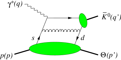
Figure 1: One of the graphs for the $\gamma^{*}p\to\bar{K}^{0}\,\Theta$ amplitude in the Bjorken limit. The large blob denotes the GPD for the $p\to\Theta$ transition and the small one the DA of the kaon.

The kinematics of the $\gamma^{*}p$ or $\gamma^{*}n$ subprocess is specified by the invariants

$$Q^{2}=-q^{2},\qquad W^{2}=(p+q)^{2},\qquad t=(p-p^{\prime})^{2},$$ (3)

with four-momenta as given in Fig. 1. We are interested in the Bjorken limit of large $Q^{2}$ at fixed $t$ and fixed scaling variable $x_{B}=Q^{2}/(2pq)$.

According to the factorization theorem for meson production [11], the Bjorken limit implies factorization of the $\gamma^{*}p$ amplitude into a perturbatively calculable subprocess at quark level, the distribution amplitude (DA) of the produced meson, and a generalized parton distribution (GPD) describing the transition from $p$ to $\Theta$ (see Fig. 1). The dominant polarization of the photon and (if applicable) the produced meson is then longitudinal, and the corresponding $\gamma^{*}p$ cross section scales like $d\sigma_{L}/(dt)\sim Q^{-6}$ at fixed $x_{B}$ and $t$, up to logarithmic corrections in $Q^{2}$ due to perturbative evolution.

We remark that pentaquarks with strangeness $S=-2$, like the $\Xi^{--}$ recently reported in [12], cannot be produced from the nucleon by this leading-twist mechanism. We also note that if the $\Theta$ had isospin $I=2$ as proposed in [13] (but not favored by the experimental analyses in [2]), leading-twist electroproduction would be isospin violating and hence tiny.

The Bjorken limit implies a large invariant mass $W$ of the hadronic final state, so that the produced baryon and meson are well separated in phase space. This provides a clean environment to study the $\Theta$ resonance, with a low background obtained of course at the price of a lower cross section than for inclusive production. Large enough $W$ in particular drives one away from kinematic reflections which could fake a $\Theta$ resonance signal, discussed in [14] for the process at hand. To illustrate this we show in Fig. 2 the smallest kinematically possible invariant masses of the $\bar{K}^{0}K^{0}$ and of the $\bar{K}^{0}p$ system in $ep\to\bar{K}^{0}K^{0}p$ with the $K^{0}p$ invariant mass fixed at $m_{\Theta}$. Here and in the following we take $m_{\Theta}=1540\,{\rm MeV}$ in numerical evaluations (our results do not change significantly if we take $m_{\Theta}=1525\,{\rm MeV}$ or $m_{\Theta}=1555\,{\rm MeV}$ instead). We also remark that strong interactions (in particular resonance) effects between the $\bar{K}^{0}$ and the $K^{0}p$ system will have a faster power falloff than $Q^{-6}$ in the $\gamma^{*}p$ cross section at fixed $x_{B}$, provided $Q^{2}$ is large enough for the analysis of the factorization theorem to apply.

Figure 2: Minimum invariant mass $M$ of $\bar{K}^{0}K^{0}$ (lower curve) and of $\bar{K}^{0}p$ (upper curve) in the process $ep\to e\bar{K}^{0}K^{0}p$ at fixed invariant mass $1540\,{\rm MeV}$ of the $K^{0}p$ system.

3 The transition GPDs and their physics

Let us take a closer look at the transition GPDs that occur in the processes we are interested in. For their definition we introduce light-cone coordinates $v^{\pm}=(v^{0}\pm v^{3})/\sqrt{2}$ and transverse components $v_{T}=(v^{1},v^{2})$ for any four-vector $v$. The skewness variable $\xi=(p-p^{\prime})^{+}/(p+p^{\prime})^{+}$ describes the loss of plus-momentum of the incident nucleon and is connected with $x_{B}$ by

$$\xi\approx\frac{x_{B}}{2-x_{B}}$$ (4)

in the Bjorken limit.

In the following we assume that the $\Theta$ has spin $J=\textstyle\frac{1}{2}$ and isospin $I=0$. Different theoretical approaches predict either $\eta_{\Theta}=1$ or $\eta_{\Theta}=-1$ for the intrinsic parity of the $\Theta$, and we will give our discussion for the two cases in parallel. The hadronic matrix elements that occur in the electroproduction processes (1) at leading-twist accuracy are

$$F_{V} = \frac{1}{2}\int\frac{dz^{-}}{2\pi}\,e^{ixP^{+}z^{-}}\langle\Theta|\,\bar{d}(-\textstyle\frac{1}{2}z)\,\gamma^{+}s(\textstyle\frac{1}{2}z)\,|p\rangle\Big{|}_{z^{+}=0,\,{z}_{T}=0}\;,$$

$$F_{A} = \frac{1}{2}\int\frac{dz^{-}}{2\pi}\,e^{ixP^{+}z^{-}}\langle\Theta|\,\bar{d}(-\textstyle\frac{1}{2}z)\,\gamma^{+}\gamma_{5}\,s(\textstyle\frac{1}{2}z)\,|p\rangle\Big{|}_{z^{+}=0,\,{z}_{T}=0}$$ (5)

with $P=\textstyle\frac{1}{2}(p+p^{\prime})$, where here and in the following we do not explicitly label the hadron spin degrees of freedom. We define the corresponding $p\to\Theta$ transition GPDs by

$$F_{V} = \frac{1}{2P^{+}}\left[H(x,\xi,t)\,\bar{u}(p^{\prime})\gamma^{+}u(p)+E(x,\xi,t)\,\bar{u}(p^{\prime})\frac{i\sigma^{+\alpha}(p^{\prime}-p)_{\alpha}}{m_{\Theta}+m_{N}}u(p)\,\right],$$

$$F_{A} = \frac{1}{2P^{+}}\left[\tilde{H}(x,\xi,t)\,\bar{u}(p^{\prime})\gamma^{+}\gamma_{5}u(p)+\tilde{E}(x,\xi,t)\,\bar{u}(p^{\prime})\frac{\gamma_{5}\,(p^{\prime}-p)^{+}}{m_{\Theta}+m_{N}}u(p)\,\right]$$ (6)

for $\eta_{\Theta}=1$ and by

$$F_{V} = \frac{1}{2P^{+}}\left[\tilde{H}(x,\xi,t)\,\bar{u}(p^{\prime})\gamma^{+}\gamma_{5}u(p)+\tilde{E}(x,\xi,t)\,\bar{u}(p^{\prime})\frac{\gamma_{5}\,(p^{\prime}-p)^{+}}{m_{\Theta}+m_{N}}u(p)\,\right],$$

$$F_{A} = \frac{1}{2P^{+}}\left[H(x,\xi,t)\,\bar{u}(p^{\prime})\gamma^{+}u(p)+E(x,\xi,t)\,\bar{u}(p^{\prime})\frac{i\sigma^{+\alpha}(p^{\prime}-p)_{\alpha}}{m_{\Theta}+m_{N}}u(p)\,\right]$$ (7)

for $\eta_{\Theta}=-1$. Notice that the tilde in our notation indicates the dependence on the spin of the hadrons, not on the spin of the quarks. The scale dependence of the matrix elements is governed by the nonsinglet evolution equations for GPDs [7, 15], with the unpolarized evolution kernels for $F_{V}$ and the polarized ones for $F_{A}$. Isospin invariance gives $\langle\Theta|\bar{d}_{\alpha}s_{\beta}|p\rangle=-\langle\Theta|\bar{u}_{\alpha}s_{\beta}|n\rangle$, so that the transition GPDs for $n\to\Theta$ and those for $p\to\Theta$ are equal up to a global sign. For simplicity we write $F_{V}$, $F_{A}$ and $H$, $E$, $\tilde{H}$, $\tilde{E}$ without labels for the transition $p\to\Theta$.

The value of $x$ determines the partonic interpretation of the GPDs. For $\xi<x<1$ the proton emits an $s$ quark and the $\Theta$ absorbs a $d$ quark, whereas for $-1<x<-\xi$ the proton emits a $\bar{d}$ and the $\Theta$ absorbs an $\bar{s}$. The region $-\xi<x<\xi$ describes emission of an $s\bar{d}$ pair by the proton. In all three cases sea quark degrees of freedom in the proton are involved. The interpretation of GPDs becomes yet more explicit when the GPDs are expressed as the overlap of light-cone wave functions for the proton and the $\Theta$. As shown in Fig. 3, the proton must be in at least a five-quark configuration for $\xi<|x|<1$ and at least a seven-quark configuration for $-\xi<x<\xi$. We emphasize however that all possible spectator configurations have to be summed over in the wave function overlap, including Fock states with additional partons in the nucleon and in the pentaquark.

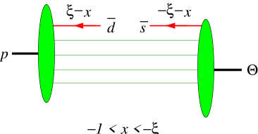
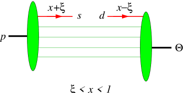
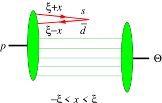
Figure 3: Wave function representation of the $p\to\Theta$ GPDs in the different regions of $x$. The blobs denote light-cone wave functions, and all possible configurations of spectator partons have to be summed over. The overall transverse position of the $\Theta$ is shifted relative to the proton as explained in [17].

As shown in [16], GPDs contain information about the spatial structure of hadrons. A Fourier transform converts their dependence on $t$ into the distribution of quarks or antiquarks in the plane transverse to their direction of motion in the infinite momentum frame. This tells us about the transverse size of the hadrons in question. The wave function overlap can also be formulated in this impact parameter representation, with wave functions specifying transverse position and plus-momentum fraction of each parton. This has in fact been done in Fig. 3, and we refer to [17] for a full discussion. We see in particular that for $\xi<|x|<1$ the transverse positions of all partons must match in the proton and the $\Theta$, including the quark or antiquark taking part in the hard scattering. For $-\xi<x<\xi$ the transverse positions of the spectator partons in the proton must match those in the $\Theta$, whereas the $s$ and $\bar{d}$ are extracted from the proton at the same transverse position (within an accuracy of order $1/Q$ set by the factorization scale of the hard scattering process). Note that small-size quark-antiquark pairs with net strangeness are not necessarily rare in the proton, as is shown by the rather large kaon pole contribution in the $p\to\Lambda$ transition (see the discussion after (27) below). In summary, the $p\to\Theta$ transition GPDs probe the partonic structure of the $\Theta$, requiring the plus-momenta and transverse positions of its partons to match with appropriate configurations in the nucleon. The helicity and color structure of the parton configurations must match as well.

We recall that for elastic transitions like $p\to p$ the analogs of the matrix elements (3) reduce to the usual parton densities in the forward limit of $\xi=0$ and $t=0$. One then has $H(x)=q(x)$, $H(-x)=-\bar{q}(x)$ and $\tilde{H}(x)=\Delta q(x)$, $\tilde{H}(-x)=\Delta\bar{q}(x)$ for $x>0$, and the positivity of parton densities results in inequalities like $|H(x)+H(-x)|\leq|H(x)-H(-x)|$ and $|\tilde{H}(x)|\leq|H(x)|$. One may expect that this hierarchy persists at least in a limited region of nonzero $\xi$ and $t$. For the $p\to\Theta$ transition the situation is different. At given $\xi$ and $t$ the combinations $F_{V}(x)-F_{V}(-x)$ and $F_{A}(x)+F_{A}(-x)$ still give the sum of the configurations in Fig. 3 with emission of a quark ($\xi<x<1$) and of an antiquark ($\xi<-x<1$), whereas $F_{V}(x)+F_{V}(-x)$ and $F_{A}(x)-F_{A}(-x)$ give their difference. In the same $x$ regions $F_{V}$ still gives the sum and $F_{A}$ the difference of configurations with positive and negative helicity of the emitted and the absorbed parton. There are however no positivity constraints now, since the $p\to\Theta$ transition GPDs do not become densities in any limit. They rather describe the correlation between wave functions of $\Theta$ and nucleon, which may be quite different. Knowledge of the relative size of the GPD combinations just discussed would in turn translate into characteristic information about the wave functions of the $\Theta$ relative to those of the proton.

In the transition GPDs we have defined, the $\Theta$ is treated as a stable hadron. The amplitude of a full process, say $ep\to e\bar{K}^{0}K^{0}p$ for definiteness, contains in addition a factor for the decay $\Theta\to K^{0}p$ and a term for the nonresonant $K^{0}p$ continuum. An alternative description is to use matrix elements analogous to (3) directly for the hadronic state $|K^{0}p\rangle$ of given invariant mass, including both resonance and continuum. The leading-twist expression of the amplitude then contains $p\to K^{0}p$ transition GPDs, which have complex phases describing the strong interactions in the $K^{0}p$ system. In the partial wave relevant for the $\Theta$ resonance, these phases will show a strong variation in the invariant $K^{0}p$ mass around $m_{\Theta}$.

4 Scattering amplitude and cross section

The scattering amplitude for longitudinal polarization of photon and meson at leading order in $1/Q$ and in $\alpha_{s}$ readily follows from the general expressions for meson production given in [9]. One has

$$\mathcal{A}_{\gamma^{*}p\to\bar{K}^{0}\,\Theta} = ie\,\frac{8\pi\alpha_{s}}{27}\,\frac{f_{K}}{Q}\,\Bigg{[}I_{K}\int_{-1}^{1}\frac{dx}{\xi-x-i\epsilon}\,\Big{(}F_{A}(x,\xi,t)-F_{A}(-x,\xi,t)\Big{)}$$

$$\hskip 42.00003pt{}+J_{K}\int_{-1}^{1}\frac{dx}{\xi-x-i\epsilon}\,\Big{(}F_{A}(x,\xi,t)+F_{A}(-x,\xi,t)\Big{)}\,\Bigg{]},$$

$$\mathcal{A}_{\gamma^{*}p\to\bar{K}^{*0}\,\Theta} = ie\,\frac{8\pi\alpha_{s}}{27}\,\frac{f_{K^{*}}}{Q}\,\Bigg{[}I_{K^{*}}\int_{-1}^{1}\frac{dx}{\xi-x-i\epsilon}\,\Big{(}F_{V}(x,\xi,t)-F_{V}(-x,\xi,t)\Big{)}$$ (8)

$$\hskip 38.00008pt{}+J_{K^{*}}\int_{-1}^{1}\frac{dx}{\xi-x-i\epsilon}\,\Big{(}F_{V}(x,\xi,t)+F_{V}(-x,\xi,t)\Big{)}\,\Bigg{]},$$

independently of the parity of the $\Theta$. Our phase conventions for meson states are fixed by

$$\langle\bar{K}^{0}(q^{\prime})|\bar{s}(0)\gamma^{\mu}\gamma_{5}\,d(0)|0\rangle = \langle K^{-}(q^{\prime})|\bar{s}(0)\gamma^{\mu}\gamma_{5}\,u(0)|0\rangle\;=\;-iq^{\prime\mu}f_{K},$$

$$\langle\bar{K}^{*0}(q^{\prime},\epsilon^{\prime})|\bar{s}(0)\gamma^{\mu}d(0)|0\rangle = \langle K^{*-}(q^{\prime},\epsilon^{\prime})|\bar{s}(0)\gamma^{\mu}u(0)|0\rangle\;=\;-i\epsilon^{\prime\mu}m_{K^{*}}f_{K^{*}},$$ (9)

where $f_{K}=160\,{\rm MeV}$, $f_{K^{*}}=(218\pm 4)\,{\rm MeV}$ [18], and $\epsilon^{\prime}$ is the polarization vector of the $K^{*}$. This differs from the convention in [9] by the factors of $-i$ on the r.h.s. In (4) we have integrals

$$I = \int_{0}^{1}dz\,\frac{1}{z(1-z)}\,\phi(z)\;=\;6\sum_{n=0}^{\infty}a_{2n},$$

$$J = \int_{0}^{1}dz\,\frac{2z-1}{z(1-z)}\,\phi(z)\;=\;6\sum_{n=0}^{\infty}a_{2n+1},$$ (10)

over the twist-two distribution amplitudes of either $\bar{K}^{0}$ or $\bar{K}^{*0}$. Our DAs are normalized to $\int_{0}^{1}dz\,\phi(z)=1$, and $z$ denotes the momentum fraction of the $s$-quark in the kaon. Because of isospin invariance $\bar{K}^{0}$ and $K^{-}$ have the same DA, as have $\bar{K}^{*0}$ and $K^{*-}$. In (4) we have used the expansion of DAs on Gegenbauer polynomials,

$$\phi(z)=6z(1-z)\sum_{n=0}^{\infty}a_{n}\,C^{3/2}_{n}(2z-1)$$ (11)

with $a_{0}=1$ due to our normalization condition. Note that odd Gegenbauer coefficients $a_{2n+1}$ are nonzero due to the breaking of flavor SU(3) symmetry. A recent estimate from QCD sum rules by Ball and Boglione [19] obtained $a_{1}^{K^{-}}=-0.18\pm 0.09$, $a_{2}^{K^{-}}=0.16\pm 0.10$ and $a_{1}^{K^{*-}}=-0.4\pm 0.2$, $a_{2}^{K^{*-}}=0.09\pm 0.05$ at a factorization scale $\mu=1\,{\rm GeV}$. Note that the sign of $a_{1}$ in both cases is such that the $s$ quark tends to carry less momentum than the light antiquark, see the discussion in [19]. In contrast, Bolz et al. [20] estimated $a_{1}^{K^{-}}$ to be of order $+0.1$ for the kaon, using results of a calculation in the Nambu-Jona-Lasinio model.

Note that the combination of GPDs going with $I_{K}$ corresponds to the difference of quark and antiquark configurations in the sense of our discussion at the end of Section 3. In contrast, the combination going with $I_{K^{*}}$ corresponds to the sum of quark and antiquark contributions. Given our ignorance about the relative sign of the transition GPDs at $x$ and $-x$ we cannot readily say whether the terms with $I$ or with $J$ tend to dominate in the amplitudes (4).

For a neutron target the scattering amplitudes read

$$\mathcal{A}_{\gamma^{*}n\to{K}^{-}\,\Theta} = -ie\,\frac{8\pi\alpha_{s}}{27}\,\frac{f_{K}}{Q}\,\Bigg{[}I_{K}\int_{-1}^{1}\frac{dx}{\xi-x-i\epsilon}\,\Big{(}F_{A}(x,\xi,t)+2F_{A}(-x,\xi,t)\Big{)}$$

$$\hskip 50.00008pt{}+J_{K}\int_{-1}^{1}\frac{dx}{\xi-x-i\epsilon}\,\Big{(}F_{A}(x,\xi,t)-2F_{A}(-x,\xi,t)\Big{)}\,\Bigg{]},$$

$$\mathcal{A}_{\gamma^{*}n\to{K}^{*-}\,\Theta} = -ie\,\frac{8\pi\alpha_{s}}{27}\,\frac{f_{K^{*}}}{Q}\,\Bigg{[}I_{K^{*}}\int_{-1}^{1}\frac{dx}{\xi-x-i\epsilon}\,\Big{(}F_{V}(x,\xi,t)+2F_{V}(-x,\xi,t)\Big{)}$$ (12)

$$\hskip 46.00012pt{}+J_{K^{*}}\int_{-1}^{1}\frac{dx}{\xi-x-i\epsilon}\,\Big{(}F_{V}(x,\xi,t)-2F_{V}(-x,\xi,t)\Big{)}\,\Bigg{]},$$

where we have used the isospin relations between the GPDs for $p\to\Theta$ and $n\to\Theta$ and between the DAs for neutral and charged kaons. Due to the different factors for a photon coupling to $d$ and $u$ quarks, the proton and neutron amplitudes involve different combinations of GPDs at $x$ and $-x$. Information on the relative size of these combinations can thus be obtained by comparing data for proton and neutron targets, given our at least qualitative knowledge about the relative size of the integrals $I$ and $J$ over meson DAs. If for example one had $F_{A}(x,\xi,t)\approx F_{A}(-x,\xi,t)$, the amplitude for $\gamma^{*}p\to\bar{K}^{0}\Theta$ would be dominated by the SU(3) breaking integral $J_{K}$ and hence be suppressed, whereas no such suppression would occur in the amplitude for $\gamma^{*}n\to K^{-}\Theta$. Comparison of $K$ and $K^{*}$ production on a given target can in turn reveal the relative size between the matrix elements $F_{A}$ and $F_{V}$.

To leading accuracy in $1/Q^{2}$ and in $\alpha_{s}$ the cross section for $\gamma^{*}p$ for a longitudinal photon on transversely polarized target is

$$\frac{d\sigma_{L}}{dt} = \frac{64\pi^{2}\alpha_{\mathit{em}}^{\phantom{2}}\alpha_{s}^{2}}{729}\,\frac{f_{K^{(*)}}^{2}}{Q^{6}}\,\frac{\xi^{2}}{1-\xi^{2}}\,(S_{U}+S_{T}\,\sin\beta),$$ (13)

where we use Hand’s convention [21] for the virtual photon flux. $\beta$ is the azimuthal angle between the hadronic plane and the transverse target spin as defined in Fig. 4. The cross section for an unpolarized target is simply obtained by omitting the $\beta$-dependent term. To have concise expressions for $S_{U}$ and $S_{T}$ we define

$$\mathcal{H}(\xi,t) = I_{K^{(*)}}\int_{-1}^{1}\frac{dx}{\xi-x-i\epsilon}\,\Big{(}H(x,\xi,t)-H(-x,\xi,t)\Big{)}$$ (14)

$$+ J_{K^{(*)}}\int_{-1}^{1}\frac{dx}{\xi-x-i\epsilon}\,\Big{(}H(x,\xi,t)+H(-x,\xi,t)\Big{)}$$

and analogous expressions $\mathcal{E}$, $\tilde{\mathcal{H}}$, $\tilde{\mathcal{E}}$ for the other GPDs. For $\eta_{\Theta}=1$ we have

$$S_{U} = (1-\xi^{2})|\tilde{\mathcal{H}}|^{2}+\frac{(m_{\Theta}-m_{N})^{2}-t}{(m_{\Theta}+m_{N})^{2}}\,\xi^{2}|\tilde{\mathcal{E}}|^{2}-\Bigg{(}\xi+\frac{m_{\Theta}-m_{N}}{m_{\Theta}+m_{N}}\Bigg{)}2\xi\,\mathrm{Re}\,(\tilde{\mathcal{E}}^{*}\tilde{\mathcal{H}})\,,$$

$$S_{T} = -\sqrt{1-\xi^{2}}\,\frac{\sqrt{t_{0}-t}}{m_{\Theta}+m_{N}}\,2\xi\,\mathrm{Im}\,(\tilde{\mathcal{E}}^{*}\tilde{\mathcal{H}})$$ (15)

for $K$ production and

$$S_{U} = (1-\xi^{2})|\mathcal{H}|^{2}-\Bigg{(}\frac{2\xi(m_{\Theta}^{2}-m_{N}^{2})+t}{(m_{\Theta}+m_{N})^{2}}+\xi^{2}\Bigg{)}|\mathcal{E}|^{2}-\Bigg{(}\xi+\frac{m_{\Theta}-m_{N}}{m_{\Theta}+m_{N}}\Bigg{)}2\xi\,\mathrm{Re}\,(\mathcal{E}^{*}\mathcal{H})\,,$$

$$S_{T} = \sqrt{1-\xi^{2}}\,\frac{\sqrt{t_{0}-t}}{m_{\Theta}+m_{N}}\,2\mathrm{Im}\,(\mathcal{E}^{*}\mathcal{H})$$ (16)

for $K^{*}$ production. If $\eta_{\Theta}=-1$ then (4) describes $K^{*}$ production and (4) describes $K$ production. We see that one cannot determine the parity of the $\Theta$ from the leading twist cross section (13) without knowledge about the dependence of $\mathcal{H}$, $\mathcal{E}$, $\tilde{\mathcal{H}}$, $\tilde{\mathcal{E}}$ on $t$ or $\xi$. The same holds for scattering on a neutron target, where one has to replace $H(-x,\xi,t)$ with $-2H(-x,\xi,t)$ in (14) and likewise change the expressions for the other GPDs, as follows from (4) and (4).

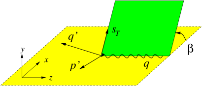
Figure 4: Definition of the azimuthal angle $\beta$ between the hadronic plane and the transverse target spin $s_{T}$ in the target rest frame. $s_{T}$ is perpendicular to the $z$-axis, which points in the direction opposite to the virtual photon momentum.

There is theoretical and phenomenological evidence that higher-order corrections in $\alpha_{s}$ and in $1/Q$ can be substantial in meson electroproduction at moderate values of $Q^{2}$, see [8, 9] for a discussion and references. For $K^{*}$ production one can in particular expect an important contribution from transverse polarization of the photon and the meson, in analogy to what has been measured for exclusive electroproduction of a $\rho^{0}$. A minimum requirement for the applicability of a leading-twist description is that $Q^{2}$ should be large compared to $-t$ and $m^{2}_{K}$ or $m_{K^{*}}^{2}$, which directly enter in the kinematics of the hard scattering process and should be negligible there. In kinematic relations, the squared baryon masses $m^{2}_{N}$ and $m_{\Theta}^{2}$ typically occur as corrections to terms of size $W^{2}$, although a complete analysis of target mass corrections in exclusive processes has not been performed yet.

There are arguments [22, 8, 9] that theoretical uncertainties from some of the corrections just discussed cancel at least partially in suitable ratios of cross sections. At the level of the leading order formulae (4) and (4) we see for instance that the scale uncertainty in $\alpha_{s}$ cancels in the ratio of cross sections on a proton and a neutron target, and that the dependence on the meson structure comes only via the ratio $J/I$. Other processes to compare with are given by $ep\to eK^{0}\Sigma^{+}$, $ep\to eK^{+}\Sigma^{0}$, $ep\to eK^{+}\Lambda$ or their analogs for vector kaons or a neutron target, with the production of either ground state or excited hyperons. Such channels may also be useful for cross checks of experimental resolution and energy calibration. Their amplitudes are given as in (4) with an appropriate replacement of matrix elements $F_{V}$ or $F_{A}$ listed in Table 1. We have used isospin invariance to replace the transition GPDs from the neutron with those from the proton. Isospin invariance further gives $F_{p\to\Sigma^{+}}=\sqrt{2}\,F_{p\to\Sigma^{0}}$.

Table 1: Combinations of transition GPDs multiplying $I$ and $J$ in the hard scattering formula (4) and its analogs for the listed channels.

$$\begin{array}[]{lll}\hline\cr\hline\cr&~{}~{}~{}~{}~{}~{}~{}~{}~{}~{}~{}~{}~{}~{}~{}I&~{}~{}~{}~{}~{}~{}~{}~{}~{}~{}~{}~{}~{}~{}~{}J\\ \hline\cr\gamma^{*}p\to\bar{K}^{0}\Theta&\phantom{-}F_{p\to\Theta}(x)-F_{p\to\Theta}(-x)&\phantom{-}F_{p\to\Theta}(x)+F_{p\to\Theta}(-x)\\ \gamma^{*}p\to K^{0}\Sigma^{+}&\phantom{-}F_{p\to\Sigma^{+}}(x)-F_{p\to\Sigma^{+}}(-x)&-[F_{p\to\Sigma^{+}}(x)+F_{p\to\Sigma^{+}}(-x)]\\ \gamma^{*}p\to K^{+}\Sigma^{0}&-[2F_{p\to\Sigma^{0}}(x)+F_{p\to\Sigma^{0}}(-x)]&\phantom{-}2F_{p\to\Sigma^{0}}(x)-F_{p\to\Sigma^{0}}(-x)\\ \gamma^{*}p\to K^{+}\Lambda&-[2F_{p\to\Lambda}(x)+F_{p\to\Lambda}(-x)]&\phantom{-}2F_{p\to\Lambda}(x)-F_{p\to\Lambda}(-x)\\ \hline\cr\gamma^{*}n\to{K}^{-}\Theta&-[F_{p\to\Theta}(x)+2F_{p\to\Theta}(-x)]&-[F_{p\to\Theta}(x)-2F_{p\to\Theta}(-x)]\\ \gamma^{*}n\to K^{+}\Sigma^{-}&\phantom{-}2F_{p\to\Sigma^{+}}(x)+F_{p\to\Sigma^{+}}(-x)&-[2F_{p\to\Sigma^{+}}(x)-F_{p\to\Sigma^{+}}(-x)]\\ \gamma^{*}n\to K^{0}\Sigma^{0}&-[F_{p\to\Sigma^{0}}(x)-F_{p\to\Sigma^{0}}(-x)]&\phantom{-}F_{p\to\Sigma^{0}}(x)+F_{p\to\Sigma^{0}}(-x)\\ \gamma^{*}n\to K^{0}\Lambda&\phantom{-}F_{p\to\Lambda}(x)-F_{p\to\Lambda}(-x)&-[F_{p\to\Lambda}(x)+F_{p\to\Lambda}(-x)]\\ \hline\cr\hline\cr\end{array}$$

For transitions within the ground state baryon octet, SU(3) flavor symmetry relates the transition GPDs to the flavor diagonal ones for $u$, $d$ and $s$ quarks in the proton [22],

$$F_{p\to\Lambda} = \frac{1}{\sqrt{6}}\,\Big{(}F^{s}_{p\to p}+F^{d}_{p\to p}-2F^{u}_{p\to p}\Big{)},$$

$$F_{p\to\Sigma^{0}} = \frac{1}{\sqrt{2}}\,\Big{(}F^{s}_{p\to p}-F^{d}_{p\to p}\Big{)}.$$ (17)

One may expect these relations to hold reasonably well, except for the distributions $\tilde{E}$, where SU(3) symmetry is strongly broken by the difference between pion and kaon mass in the respective pole contributions (see the following section). In the approximation of SU(3) symmetry, comparison of $\Theta$ production with the corresponding hyperon channels would thus compare the $N\to\Theta$ transition GPDs with the GPDs of the nucleon itself.

5 Kaon pole contributions

In analogy to the well-known pion exchange contribution to the elastic nucleon GPDs, the axial vector matrix elements $F_{A}$ for the transition between nonstrange and strange baryons receive a contribution from kaon exchange in the $t$-channel, as shown in Fig. 5. It can be expressed in terms of the kaon distribution amplitude and the appropriate baryon-kaon coupling if $t=m_{K}^{2}$. This is of course outside the physical region for our electroproduction processes, where the contribution from the kaon pole is expected to be less and less dominant for increasing $-t$. With this caveat in mind we will now discuss the kaon pole contribution to the $N\to\Theta$ GPDs, as this can be done without a particular dynamical model for the $\Theta$.

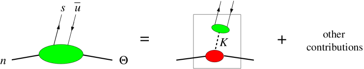
Figure 5: Kaon pole contribution to the $n\to\Theta$ transition GPDs in the region $-\xi<x<\xi$.

We recall at this point that the minimal kinematically allowed value of $-t$ at given $\xi$,

$$-t_{0}=\frac{2\xi^{2}(m_{\Theta}^{2}+m_{N}^{2})+2\xi(m_{\Theta}^{2}-m_{N}^{2})}{1-\xi^{2}},$$ (18)

is not so small in typical kinematics of fixed target experiments. This is shown in Fig. 6, where we have replaced $\xi$ with $x_{B}$ using the relation (4) valid in Bjorken kinematics. We also show the corresponding values of $-t_{0}$ for the transition from the nucleon to a ground state $\Sigma$ or $\Lambda$.

Figure 6: Minimum kinematically allowed value of $-t$ at given $x_{B}$ for the transitions $N\to\Theta$, $N\to\Sigma$, $N\to\Lambda$, see (4) and (18).

We define the $\Theta NK$ coupling through

$$\mathcal{L}=ig_{\Theta NK}K_{d}(\bar{\Theta}\gamma_{5}p)-ig_{\Theta NK}K_{u}(\bar{\Theta}\gamma_{5}n)+\textrm{c.c.}$$ (19)

if $\eta_{\Theta}=1$, and through

$$\mathcal{L}=ig_{\Theta NK}K_{d}(\bar{\Theta}p)-ig_{\Theta NK}K_{u}(\bar{\Theta}n)+\textrm{c.c.}$$ (20)

if $\eta_{\Theta}=-1$. Here $K_{d}$ denotes the field that creates a $\bar{K}^{0}$ and $K_{u}$ the one creating a $K^{-}$. The factor of $i$ in (20) is dictated by time reversal invariance, since we choose the phase of the $\Theta$ field such that it has the same transformation under time reversal as the nucleon field. Then the GPDs defined in (3) are real valued. The above definitions can be rewritten in terms of the vector or axial vector current using the free Dirac equation for the $\Theta$ and the nucleon fields. Using the method of [23] we obtain kaon pole contributions

$$\xi\tilde{E}_{\mathrm{pole}} = \frac{g_{\Theta NK}f_{K}(m_{\Theta}+m_{N})}{m_{K}^{2}-t}\,\frac{1}{2}\phi\Big{(}\frac{x+\xi}{2\xi}\Big{)}$$

$$\tilde{H}_{\mathrm{pole}} = H_{\mathrm{pole}}\;=\;E_{\mathrm{pole}}\;=\;0$$ (21)

for $\eta_{\Theta}=1$ and

$$E_{\mathrm{pole}} = -H_{\mathrm{pole}}=\frac{g_{\Theta NK}f_{K}(m_{\Theta}+m_{N})}{m_{K}^{2}-t}\,\frac{1}{2}\phi\Big{(}\frac{x+\xi}{2\xi}\Big{)}$$

$$\tilde{H}_{\mathrm{pole}} = \tilde{E}_{\mathrm{pole}}\;=\;0$$ (22)

for $\eta_{\Theta}=-1$, where it is understood that $x$ is limited to the region between $-\xi$ and $\xi$, and where $\phi$ is the same kaon distribution amplitude we have encountered earlier. At the level of the amplitudes (4) and (4) for $K$ production one finds

$$\mathcal{A}_{\gamma^{*}p\to\bar{K}^{0}\,\Theta}^{\mathrm{pole}} = ie\,\bar{u}(p^{\prime})\gamma_{5}\,{u}(p)\,\frac{g_{\Theta NK}}{m_{K}^{2}-t}\,QF_{\bar{K}^{0}}(Q^{2}),$$

$$\mathcal{A}_{\gamma^{*}n\to{K}^{-}\,\Theta}^{\mathrm{pole}} = -ie\,\bar{u}(p^{\prime})\gamma_{5}\,{u}(p)\,\frac{g_{\Theta NK}}{m_{K}^{2}-t}\,QF_{K^{-}}(Q^{2})$$ (23)

for $\eta_{\Theta}=1$, whereas for $\eta_{\Theta}=-1$ one simply has to replace $\bar{u}(p^{\prime})\gamma_{5}\,{u}(p)$ with $\bar{u}(p^{\prime}){u}(p)$ in both relations. Here

$$F_{\bar{K}^{0}}(Q^{2}) = -\frac{2\pi\alpha_{s}}{9}\,\frac{f_{K}^{2}}{Q^{2}}\,\frac{4}{3}I_{K}J_{K}$$

$$F_{K^{-}}(Q^{2}) = -\frac{2\pi\alpha_{s}}{9}\,\frac{f_{K}^{2}}{Q^{2}}\,\Big{(}I_{K}^{2}-\frac{2}{3}I_{K}J_{K}+J_{K}^{2}\Big{)}$$ (24)

are the elastic kaon form factors at leading accuracy in $1/Q^{2}$ and $\alpha_{s}$. We note that the relations (5) remain valid beyond this approximation, which in analogy to the pion form factor we expect to receive important corrections at moderate $Q^{2}$, see [9] for references. The form factors are normalized as $F_{K^{-}}(0)=-1$ and $F_{\bar{K}^{0}}(0)=0$, and at nonzero $t$ the neutral kaon form factor is only nonzero thanks to flavor SU(3) breaking. The contribution of the squared kaon pole amplitude to the $\gamma^{*}p\to\bar{K}^{0}\Theta$ or $\gamma^{*}n\to K^{-}\Theta$ cross section finally reads

$$\frac{d\sigma_{L}}{dt}\Bigg{|}_{\mathrm{pole}}=\alpha_{\mathit{em}}^{\phantom{2}}\frac{F_{K}^{2}(Q^{2})}{Q^{2}}\,\frac{x_{B}^{2}}{4(1-x_{B})}\;g_{\Theta NK}^{2}\,\frac{(m_{\Theta}-\eta_{\Theta}m_{N})^{2}-t}{(m_{K}^{2}-t)^{2}},$$ (25)

where $F_{K}$ is the appropriate form factor for the $\bar{K}^{0}$ or the $K^{-}$. Of course, the pole contribution (5) also appears in the cross section via its interference with the non-pole parts of the amplitude, which we cannot estimate at this point.

For kinematical reasons $\Theta\to K^{0}p$ and $\Theta\to K^{+}n$ are the only strong decays of the $\Theta$, so that its total width $\Gamma_{\Theta}$ translates to a good accuracy into a value of $g^{2}_{\Theta NK}$,

$$\Gamma_{\Theta}=\frac{g^{2}_{\Theta NK}}{4\pi}\,k\;\frac{(m_{\Theta}-\eta_{\Theta}m_{N})^{2}-m_{K}^{2}}{m_{\Theta}^{2}},$$ (26)

where $k\approx 268\,{\rm MeV}$ is the momentum of the decay nucleon in the $\Theta$ rest frame. Taking an indicative value of $\Gamma_{\Theta}=10\,{\rm MeV}$ we obtain $g_{\Theta NK}^{2}/(4\pi)=0.77$ for $\eta_{\Theta}=1$ and $g_{\Theta NK}^{2}/(4\pi)=0.015$ for $\eta_{\Theta}=-1$. The squared couplings corresponding to different values of $\Gamma_{\Theta}$ are readily obtained by simple rescaling.

Figure 7: The kaon pole factor $G(t)$ defined in (27) and evaluated for $\Gamma_{\Theta}=10\,{\rm MeV}$ and $\eta_{\Theta}=1$, and the analogous factors for the transitions $p\to\Sigma^{0}$ and $p\to\Lambda$. The same factors appear in the kaon pole contributions to $p\to\Theta$, $n\to\Sigma^{0}$ and $n\to\Lambda$.

To be insensitive to the theoretical uncertainties in evaluating the kaon form factors, we compare in the following the kaon pole contributions to different baryon transitions. In Fig. 7 we show the factor

$$G(t)=g_{\Theta NK}^{2}\,\frac{(m_{\Theta}-\eta_{\Theta}m_{N})^{2}-t}{(m_{K}^{2}-t)^{2}}$$ (27)

appearing in the pole contribution (25) to the $\gamma^{*}n\to K^{-}\Theta$ cross section, as well as its analogs for the pole contributions to $\gamma^{*}p\to K^{+}\Sigma^{0}$ and to $\gamma^{*}p\to K^{+}\Lambda$. Due to isospin invariance the corresponding factor for $\gamma^{*}n\to K^{+}\Sigma^{-}$ is twice as large as for $\gamma^{*}p\to K^{+}\Sigma^{0}$. Following [24] we take $g_{\Sigma NK}^{2}/(4\pi)=1.2$ and $g_{\Lambda NK}^{2}/(4\pi)=14$ for the couplings between the proton and the neutral hyperons. As an indication of their uncertainties one may compare these values with those given in [25], namely $g_{\Sigma NK}^{2}/(4\pi)=1.6$ and $g_{\Lambda NK}^{2}/(4\pi)=10.6$. We remark that according to the estimates of [24], the overall cross section for $\gamma^{*}p\to K^{+}\Lambda$ is comparable in size to the one for $\gamma^{*}p\to\pi^{+}n$ in kinematics where both processes receive substantial contributions from the kaon or pion pole.

Note that the much smaller coupling for a negative-parity $\Theta$ is partially compensated in the kaon pole contribution to the cross section by a larger kinematic factor in the numerator of (25). The ratio of the factors $G(t)$ for $\eta_{\Theta}=-1$ and for $\eta_{\Theta}=1$ is shown in Fig. 8. Given the presence of contributions not due to the kaon pole it is not clear whether one could use the measured size and $t$ dependence of the cross section to infer on the parity of the $\Theta$.

Figure 8: Ratio of the kaon pole cross sections (25) for the cases $\eta_{\Theta}=-1$ and $\eta_{\Theta}=1$ at given $\Gamma_{\Theta}$.

The factors $G(t)$ shown in Fig. 7 also describe the neutral kaon pole contributions in $\gamma^{*}p\to\bar{K}^{0}\Theta$, $\gamma^{*}n\to K^{0}\Sigma^{0}$ and $\gamma^{*}n\to K^{0}\Lambda$. Compared with the respective charged kaon pole contributions in $\gamma^{*}n\to{K}^{-}\Theta$, $\gamma^{*}p\to K^{+}\Sigma^{0}$ and $\gamma^{*}p\to K^{+}\Lambda$, they are significantly suppressed by a factor $(F_{\bar{K}^{0}}/F_{K^{-}})^{2}$ at cross section level. This factor is about 0.03 if we take the leading-order expressions (5) of the form factors together with the estimates of [19] for the Gegenbauer coefficients $a_{1}$ and $a_{2}$ in the kaon DA, given below (11).

6 Conclusions

We have investigated exclusive electroproduction of a $\Theta^{+}$ pentaquark on the nucleon at large $Q^{2}$, large $W^{2}$ and small $t$. Such a process provides a rather clean environment to study the structure of pentaquark at parton level, in the form of well defined hadronic matrix elements of quark vector or axial vector currents. In parton language, these matrix elements describe how well parton configurations in the $\Theta$ match with appropriate configurations in the nucleon (see Fig. 3). Their dependence on $t$ gives information about the size of the pentaquark. Channels with production of pseudoscalar or vector kaons and with a proton or neutron target carry complementary information. The transition to the $\Theta$ requires sea quark degrees of freedom in the nucleon, and we hope that theoretical approaches including such degrees of freedom will be able to evaluate the matrix elements given in (3). Candidates for this may for instance be the chiral quark-soliton model or lattice QCD, both of which have been used to calculate the corresponding matrix elements for elastic nucleon transitions, see [26] and [27].

In order to obtain observably large cross sections one may be required to go to rather modest values of $Q^{2}$, where the leading approximation in powers of $1/Q^{2}$ and of $\alpha_{s}$ on which we based our analysis receives considerable corrections. The associated theoretical uncertainties should be alleviated by comparing $\Theta$ production to the production of $\Sigma$ or $\Lambda$ hyperons as reference channels. In any case, even a qualitative picture of the overall magnitude and relative size of the different hadronic matrix elements accessible in the processes we propose would give information about the structure of pentaquarks well beyond the little we presently know about these intriguing members of the QCD spectrum.

References

-
[1]
T. Nakano et al. [LEPS Collaboration],
Phys. Rev. Lett. 91, 012002 (2003)
[hep-ex/0301020];
S. Stepanyan et al. [CLAS Collaboration], hep-ex/0307018;
V. V. Barmin et al. [DIANA Collaboration], Phys. Atom. Nucl. 66, 1715 (2003) [hep-ex/0304040];
A. E. Asratyan, A. G. Dolgolenko and M. A. Kubantsev, hep-ex/0309042. -
[2]
J. Barth et al. [SAPHIR Collaboration],
hep-ex/0307083;
V. Kubarovsky et al. [CLAS Collaboration], hep-ex/0311046;
A. Airapetian et al. [HERMES Collaboration], hep-ex/0312044. - [3] D. Diakonov, V. Petrov and M. V. Polyakov, Z. Phys. A 359, 305 (1997) [hep-ph/9703373].
-
[4]
M. Praszalowicz, in: M. Jezabek and M. Praszalowicz (Eds.),
Skyrmions and Anomalies, World Scientific, Singapore, 1987,
p. 112;
Phys. Lett. B 575, 234 (2003)
[hep-ph/0308114];
H. Weigel, Eur. Phys. J. A 2, 391 (1998) [hep-ph/9804260]. -
[5]
M. Karliner and H. J. Lipkin,
hep-ph/0307243;
R. L. Jaffe and F. Wilczek, hep-ph/0307341;
C. E. Carlson, C. D. Carone, H. J. Kwee and V. Nazaryan, Phys. Lett. B 573, 101 (2003) [hep-ph/0307396]. -
[6]
F. Csikor, Z. Fodor, S. D. Katz and T. G. Kovacs,
hep-lat/0309090;
S. Sasaki, hep-lat/0310014. -
[7]
D. Müller, D. Robaschik, B. Geyer, F. M. Dittes and
J. Hořejši,
Fortschr. Phys. 42, 101 (1994)
[hep-ph/9812448];
X. D. Ji, Phys. Rev. Lett. 78, 610 (1997) [hep-ph/9603249];
A. V. Radyushkin, Phys. Rev. D56, 5524 (1997) [hep-ph/9704207]. - [8] K. Goeke, M. V. Polyakov and M. Vanderhaeghen, Prog. Part. Nucl. Phys. 47, 401 (2001) [hep-ph/0106012].
- [9] M. Diehl, Phys. Rept. 388, 41 (2003) [hep-ph/0307382].
- [10] E. R. Berger, M. Diehl and B. Pire, Phys. Lett. B 523, 265 (2001) [hep-ph/0110080].
- [11] J. C. Collins, L. Frankfurt and M. Strikman, Phys. Rev. D 56, 2982 (1997) [hep-ph/9611433].
- [12] C. Alt et al. [NA49 Collaboration], hep-ex/0310014.
- [13] S. Capstick, P. R. Page and W. Roberts, Phys. Lett. B 570, 185 (2003) [hep-ph/0307019].
- [14] A. R. Dzierba, D. Krop, M. Swat, S. Teige and A. P. Szczepaniak, hep-ph/0311125.
-
[15]
J. Blümlein, B. Geyer and D. Robaschik,
Phys. Lett. B 406, 161 (1997)
[hep-ph/9705264];
A. V. Belitsky, A. Freund and D. Müller, Nucl. Phys. B 574, 347 (2000) [hep-ph/9912379]. -
[16]
M. Burkardt,
Phys. Rev. D 62, 071503 (2000),
Erratum-ibid. D 66, 119903 (2002)
[hep-ph/0005108];
J. P. Ralston and B. Pire, Phys. Rev. D 66, 111501 (2002). - [17] M. Diehl, Eur. Phys. J. C 25, 223 (2002), Erratum-ibid. C 31, 277 (2003) [hep-ph/0205208].
- [18] M. Beneke and M. Neubert, Nucl. Phys. B 675, 333 (2003) [hep-ph/0308039].
- [19] P. Ball and M. Boglione, Phys. Rev. D 68, 094006 (2003) [hep-ph/0307337].
- [20] J. Bolz, P. Kroll and G. A. Schuler, Eur. Phys. J. C 2, 705 (1998) [hep-ph/9704378].
- [21] L. N. Hand, Phys. Rev. 129, 1834 (1963).
- [22] L. L. Frankfurt, P. V. Pobylitsa, M. V. Polyakov and M. Strikman, Phys. Rev. D 60, 014010 (1999) [hep-ph/9901429].
- [23] L. Mankiewicz, G. Piller and A. Radyushkin, Eur. Phys. J. C 10, 307 (1999) [hep-ph/9812467].
- [24] L. L. Frankfurt, M. V. Polyakov, M. Strikman and M. Vanderhaeghen, Phys. Rev. Lett. 84, 2589 (2000) [hep-ph/9911381].
- [25] M. Guidal, J.-M. Laget and M. Vanderhaeghen, Phys. Rev. C 68, 058201 (2003) [hep-ph/0308131].
-
[26]
V. Y. Petrov, P. V. Pobylitsa, M. V. Polyakov, I. Börnig, K. Goeke
and C. Weiss,
Phys. Rev. D 57, 4325 (1998)
[hep-ph/9710270];
M. Penttinen, M. V. Polyakov and K. Goeke, Phys. Rev. D 62, 014024 (2000) [hep-ph/9909489]. -
[27]
QCDSF Collaboration, M. Göckeler et al.,
hep-ph/0304249;
LHPC Collaboration, P. Hägler et al., Phys. Rev. D 68, 034505 (2003) [hep-lat/0304018].