Abstract

This review, prepared for the 2002 Review of Particle Physics together with F.J. Gilman and K. Kleinknecht, summarizes experimental inputs and theoretical conclusions on the present status of the CKM mixing matrix, and on the CP violating phase $\delta_{{}_{13}}$. Experimental data are consistent with each other and with a phase of $\delta_{{}_{13}}=59^{o}\pm 13^{o}$.

Abstract

The value of the $V_{ud}$ matrix element of the Cabibbo-Kobayashi-Maskawa matrix can be derived from nuclear superallowed beta decays, neutron decay and pion beta decay. Today, the most precise value of $V_{ud}$ ($\pm 0.05\%$) comes from the nuclear decays; and its precision is limited not by experimental error but by the estimated uncertainty in theoretical corrections, which themselves are of order 1%. When combined with the best values of $V_{us}$ and $V_{ub}$, the results differ at the 98% confidence limit from the unitarity condition for the CKM matrix. This talk outlines the current status of both the experimental data and the calculated correction terms, and presents an overview of experiments currently underway to reduce the uncertainty in those correction terms that depend on nuclear structure.

Abstract

This article gives a brief summary of radiative corrections with a new analysis of neutron $\beta$-decay.

Abstract

The neutron life time $\tau_{n}$ was measured by storage of ultracold neutrons (UCN) in a material bottle covered with Fomblin oil. The inelastically scattered neutrons were detected by surrounding neutron counters monitoring the UCN losses due to upscattering at the bottle walls. Comparing traps with different surface to volume ratios the free neutron life time was deduced. Consistent results for different bottle temperatures yielded $\tau_{n}\left[\sec\right]=885.4\pm 0.9_{stat}\pm 0.4_{syst}.$

Abstract

Measurements by various international groups of researchers determine the strength of the weak interaction of the neutron, which gives us unique information on the question of the quark mixing. Neutron $\beta$-decay experiments now challenge the Standard Model of elementary particle physics with a deviation, 2.7 times the stated error.

Abstract

Decays of W^± bosons produced at LEP2 have been used to measure the Cabibbo-Kobayashi-Maskawa matrix element $|\rm V_{cs}|$ with a precision of 1.3% without the need of a form factor. The same data set has been used to test the unitarity of the first two rows of the matrix at the 2% level. At a future $\rm e^{+}e^{-}$ linear collider, with a data sample of few million of W decays a precision of 0.1% can be reached.

Abstract

We report preliminary working results of the PIBETA experiment analysis for pion beta decay ($\pi\beta$), $\pi^{+}\to\pi^{0}e^{+}\nu$, and for radiative pion decay (RPD) $\pi^{+}\to e^{+}\nu\gamma$. The former is in excellent agreement with the SM predictions at the 1 % accuracy level. The latter, an important background for the $\pi\beta$ channel, shows an intriguing departure from the basic V$-$A description.

Abstract

From $K^{+}_{e3}$ and $K_{L,e3}$ decays, $V_{us}$ can be determined to be $0.220\pm 0.003$. If $SU_{3}$ symmetry is invoked, semileptonic hyperon decays offer an independent determination $V_{us}\,=\,0.223\pm 0.004$. The unknown effects of $SU_{3}$ symmetry breaking make this result less safe than the $K_{e3}$ result.

Abstract

The project which is the subject of this talk is to be carried out by a collaboration of several groups of scientists working in the Institutes of USA and Russia.

Abstract

In this paper we briefly describe the motivation and construction of our new neutron decay spectrometer aSPECT. The goal is to enable us to measure the neutrino-electron-correlation coefficient $a$ in the decay of the free neutron with unprecedented accuracy. We summarize the systematic uncertainties of our spectrometer.

Abstract

We describe an instrument ”The New Perkeo” which is under development in Heidelberg and which will serve to measure neutron decay correlation coefficients using a pulsed cold neutron beam. The new scheme allows to eliminate the four leading error sources typical for such experiments, while vastly increasing statistical accuracy.

Abstract

At the Kernfysisch Versneller Instituut (KVI) in Groningen, NL, a new facility (TRI$\mu$P) is under development. It aims for producing, slowing down and trapping of radioactive isotopes in order to perform accurate measurements on fundamental symmetries and interactions. A spectrum of radioactive nuclids will be produced in direct, inverse kinematics of fragmentation reactions using heavy ion beams from the superconducting AGOR cyclotron. The research programme pursued by the local KVI group includes precision studies of nuclear $\beta$-decays through $\beta$–neutrino (recoil nucleus) momentum correlations in weak decays and searches for permanent electric dipole moments in heavy atomic systems. The facility in Groningen will be open for use by the worldwide community of scientists.

Abstract

We report progress towards a measurement of the neutron lifetime using magnetically trapped ultracold neutrons (UCN). UCN are produced by inelastic scattering of cold (0.89 nm) neutrons in a reservoir of superfluid ⁴He and confined in a three-dimensional magnetic trap. As the trapped neutrons decay, recoil electrons generate scintillations in the liquid He, which are detectable with greater than 90 % efficiency. The number of UCN decays vs. time will be used to determine the neutron beta-decay lifetime.

Abstract

We have measured the neutron decay lifetime by the absolute counting neutron decay recoil protons that were confined in a quasi-Penning trap. The neutron beam fluence was measured by capture in a thin ⁶LiF foil detector with known absolute efficiency. The combination of these measurements gives the neutron lifetime: $\tau_{n}=(886.8\pm 1.2{\rm[stat]}\pm 3.2{\rm[sys]})$ s, which is the most precise neutron lifetime determination to data using an in-beam method.

Abstract

A trap for neutrons with superconducting magnets - planned by the UCN group at the Physics Department of Technische Universität München - shall serve to measure the neutron lifetime. Magnetic trapping is a method complementary to that usually employed in recent years, the trapping of neutrons in bottles with material walls. It avoids the problems with neutron losses by wall collisions. With a volume of about 900 dm³ the arrangement allows to store around $10^{6}$ neutrons at the high-flux reactor of ILL, Grenoble, and orders of magnitude more with the new UCN source of the reactor FRM-II at Arching.

Abstract

We propose a new method of double super mirror polarizers in crossed geometry for neutron beam polarization. With such a geometry a beam polarization of 99.60(5)% without any significant spatial and wavelength dependence between 3 and 10 Å could be demonstrated.

Abstract

It is important to take into account the radiative corrections in precision beta decay analysis. The photon bremsstrahlung calculation in beta decays with small decay energy is free from strong interaction uncertainties, it is mainly QED result. These photons change the beta decay kinematics, it is important to take into consideration this effect, in order to obtain meaningful radiative corrections. The model independent part of the radiative correction is reliable, sensitive to the experimental details, and it is this part which changes the spectrum shapes and asymmetries. The model dependent correction can be absorbed, to a good approximation, into effective form factors. The dominant asymptotic part is reliable and universal, but the smaller non-asymptotic part contains non-perturbative strong interaction uncertainties, and it can depend on the decay type.

Abstract

Precision measurements of neutron decay observables impact a broad array of “new” physics searches. I discuss how the correlation coefficients of neutron $\beta$-decay, the neutron lifetime, and studies of neutron radiative $\beta$-decay can impact searches for non-V-A currents and new sources of CP violation.

Abstract

Radiative corrections to the neutron $\beta-$decay are calculated with consistent allowance for electroweak interactions accordingly the Weinberg-Salam theory. The effect of strong interactions is parameterized by introducing the weak nucleon transition current. The radiative corrections to the total decay probability $W$ and to the asymmetry coefficient of the electron momentum distribution $A$ constitute: $\delta{W}{\approx}8{\%}\,,\,\,\delta{A}{\approx}-2{\%}$. The accuracy attainable in the calculation proves to be $\sim{0.1{\%}}$

Abstract

We studied the effect of isospin impurity on the super-allowed Fermi $\beta$ decay using microscopic HF and RPA (or TDA) model taking into account CSB and CIB interactions. It is found that the super- allowed transitions between odd-odd $J$=0 nuclei and even-even $J$=0 nuclei are quenched because of the cancellation of the isospin impurity effects of mother and daughter nuclei. An implication of the calculated Fermi transition rate on the unitarity of Cabibbo-Kobayashi-Maskawa mixing matrix is also discussed.

Abstract

We describe the techniques used in lattice evaluations of hadronic matrix elements like the neutron decay constant $g_{A}$. Recent results for $g_{A}$ are presented and the influence of the finite quark mass and the finite volume on the determination of $g_{A}$ is briefly discussed.

Abstract

We report on the physics potential of a proposed conversion of the CESR machine and the CLEO detector to a charm and QCD factory: “CLEO-c and CESR-c” that will make crucial contributions to quark flavor physics this decade, and may offer our best hope for mastering non-perturbative QCD, which is essential if we are to understand strongly coupled sectors in the new physics that lies beyond the Standard Model. Of particular relevance to this workshop CLEO-c will make a precise measurement of $V_{cd}$ that can be combined with the beautiful measurements of $V_{ud}$ discussed elsewhere in these proceedings to test of the unitarity of the first column of the CKM matrix.

Abstract

The KLOE experiment has been running since April 1999 at the DA$\Phi$NE e⁺-e^- collider at a center of mass energy equal to the $\phi$-meson mass. The luminosity integrated up to September 2002 is $\sim 500~{}~{}pb^{-1}$. Perspectives on the measurement of the $V_{us}$ CKM-matrix element with the KLOE detector,using both charged and neutral kaon semileptonic decays, are presented.

Abstract

At PSI, we build a new type of ultracold neutron (UCN) source, based on the spallation process. The essential elements of the new source are a pulsed proton beam with a high intensity (I${}_{p}\geq$ 2mA) and a very low duty cycle (1 %), a heavy element spallation target and a moderator consisting of solid deuterium kept at a temperature of about 6 K. Recent experimental studies of the production of ultracold neutrons in solid deuterium open prospects for densities of 3000 ultracold neutrons per cm³.

Abstract

A two coil resonance method is discussed for the measurement of possible P, T-violation effects in the interaction of low-energy neutrons with polarized nuclei. It is shown that a neutron phase depending asymmetry has a direct connection with the T-odd amplitude and can be a measure of breaking T-invariance.

Abstract

In neutron beta decay, the triple correlation between the neutron spin and the momenta of electron and antineutrino ($D$ coefficient) tests for a violation of time reversal invariance beyond the Standard model mechanism of CP violation. We present a new preliminary limit for this correlation which was obtained by the Trine experiment: $D_{\rm prel.}=(-3.1\pm 6.2^{\rm stat}\pm 4.7^{\rm syst}\pm 4.7^{\rm syststat})\cdot 10^{-4}$.

Abstract

An experiment aiming at the simultaneous determination of the two transversal polarization components of electrons emitted in the decay of free, polarized neutrons is underway at the Paul Scherrer Institute, Villigen, Switzerland. A non-zero value of $R$ due to the polarization component, which is perpendicular to the plane spanned by the spin of the decaying neutron and the electron momentum, would signal a violation of time reversal symmetry and thus physics beyond the Standard Model (SM). The value of $N$, given by the transverse polarization component within that plane, is expected to be finite. The measurement of $N$ both probes the SM and serves as an important systematic check of the apparatus for the $R$-measurement. Using the Mott scattering polarimetry technique, the anticipated accuracy of $5\times 10^{-3}$ should be achieved within a few months of data taking.

Abstract

The decay of free neutrons is a simple system to study the weak interaction in detail and to search for physics beyond the Standard Model. In particular, the beta asymmetry A is well suited to test the unitarity condition of the quark mixing CKM matrix. The neutrino asymmetry B is sensitive to the existence of right handed currents.
The spectrometer PERKEO has measured the correlations A and B. We developed a technique which allows us to register both electron and proton in the same detector. This gives us access to a sensitive and systematically clean method for a B measurement.

Abstract

A brief overview is given of the most important results of the workshop, with special emphasis on the possibilities for future advances in the field of weak interaction physics offered by experiments in neutron decay.

The fundamental constituents of matter are quarks and leptons. The quarks which are involved in the process of weak interaction mix and this mixing is expressed in the so-called “Cabibbo–Kobayashi–Maskawa” (CKM) matrix. The presently poorly satisfied unitarity condition for the CKM matrix presents a puzzle in which a deviation from unitarity may point towards new physics.

The two day workshop Quark-Mixing, CKM-Unitarity was held in Heidelberg (Germany) from 19 to 20 September 2002. The workshop reviewed the information to date on the inputs for the unitarity check from the experimental and theoretical side. The Standard Model does not predict the content of the CKM matrix and the value of individual matrix elements is determined from weak decays of individual quarks. Especially the value of $V_{ud}$, the first matrix element, is subject to scrutiny. $V_{ud}$ has been derived from a series of experiments on superallowed nuclear $\beta$-decay measurements, neutron $\beta$-decay and pion $\beta$-decay. With the information from nuclear and neutron $\beta$-decay for the first quark generation and from K and hyperon-decays for the second generation, the unitarity-check fails significantly for unknown reasons. This workshop is an attempt to provide an opportunity for clarification of this situation on the experimental and theoretical side.

Accordingly, these proceedings are devoted to these topics:

$\bullet$ Unitarity of the CKM matrix
         $\bullet$ First quark flavor decays: nuclear $\beta$-decays, neutron $\beta$-decay, $\pi$–decay
         $\bullet$ Radioactive beams
         $\bullet$ Second quark flavor decays: kaon decays, hyperon decays
         $\bullet$ Standard theory – QED, electroweak and hadronic corrections
         $\bullet$ New possibilities for experiments and facilities
         $\bullet$ T- and CP-violation

With these proceedings, we present both a review of the experimental and theoretical information on quark-mixing with focus on the first quark generation. The papers present new findings on these topics in the context of what is known so far. Besides this, about half a dozen new neutron-decay instruments being planned or under construction are presented. Better neutron sources, in particular for high fluxes of cold and high densities of ultra-cold neutrons will boost fundamental studies in these fields. The workshop included invited talks and a panel discussion. The results of the panel discussion are published in “The European Physical Journal”.

The editors wish to dedicate these proceedings to Prof. Dirk Dubbers on the occasion of his 60th birthday. For many years he has given advice and support to the “Atom and Neutron Physics Group” at the University of Heidelberg Institute of Physics.

We would like to thank all participants and the programme committee members T. Bowles (LANL), W. Marciano (Brookhaven), A. Serebrov (PNPI), D. Dubbers (Heidelberg) and O. Nachtmann (Heidelberg). We would like to express our gratitude to C. Krämer and F. Schneyder, who have devoted a great deal of their time and energy to making this meeting a success.

This workshop was sponsored by the Deutsche Forschungsgemeinschaft (German Research Foundation).

Heidelberg, September 2003 Hartmut Abele
Daniela Mund

Contents

1. ‣ Status of the Cabibbo-Kobayashi-Maskawa Quark-Mixing Matrix
   1. 1 The CKM Matrix
   2. 2 Brief summary of experimental results
      1. 2.1 Tree level processes
      2. 2.2 Loop level processes
   3. 3 Determination of the CKM matrix
2. References
3. 4 Introduction
4. 5 Current status
5. 6 Future prospects
6. References
7. 7 One and Two Loop Electroweak Corrections
8. 8 Neutron Decay in the Context of Nuclear Physics
   1. 8.1 The Weak Interaction in Nuclei
   2. 8.2 Neutron Decay Parameters
   3. 8.3 Measurement of the Neutron Lifetime
   4. 8.4 Neutron Lifetime and the Big Bang
   5. 8.5 Application to Solar Astrophysics
   6. 8.6 Determination of the Weak Coupling Constants
9. 9 Neutron Decay in the Context of Particle Physics
   1. 9.1 The Cabibbo-Kobayashi-Maskawa Matrix
   2. 9.2 Neutron Decay in the Standard Model
10. 10 The Correlation Coefficients in Neutron Decay
    1. 10.1 Polarized Neutron Decay
    2. 10.2 Non-Standard Model Contributions to the Correlation Coefficients
11. 11 Measurement of the Correlation Coefficients
    1. 11.1 The Electron-Antineutrino Angular Correlation Coefficient $a$
    2. 11.2 The Electron-Neutron Spin Asymmetry Coefficient $A$
    3. 11.3 The Antineutrino-Neutron Spin Asymmetry Coefficient B
    4. 11.4 The Triple Correlation Coefficient D
12. 12 Additional Experimental Possibilities
    1. 12.1 The Proton-Neutron Spin Asymmetry Coefficient $\alpha$
    2. 12.2 Two-Body Decay of the Neutron and Right-Handed Currents
    3. 12.3 Radiative Neutron Decay
13. References
14. 13 Introduction
15. 14 Basic idea of the experimental method
16. 15 Method for a broad UCN energy spectrum
17. 16 The experiment
18. 17 Evaluation of the data and result
19. 18 Conclusion
20. 19 Acknowledgments
21. 20 The Standard Model, Quark-Mixing and the CKM Matrix
22. 21 Neutron-$\beta$-Decay
23. 22 The Experiment PERKEO and the Result for $|V_{ud}|$
24. 23 The future
25. 24 Summary
26. 25 Introduction
27. 26 $|V_{\rm{cs}}|$ from hadron decays
28. 27 $|V_{\rm{cs}}|$ from W decays
    1. 27.1 $|V_{\rm{cs}}|$ from charm production rate
    2. 27.2 $|V_{\rm{cs}}|$ from W leptonic branching fraction
    3. 27.3 $|V_{\rm{cs}}|$from $\rm W\to cs$
29. 28 Conclusion and future prospective
30. References
31. 29 Experiment Goals and Motivation
32. 30 Experimental Method
33. 31 First Results: Pion Beta Decay
34. 32 First Results: Radiative Pion Decay
35. 33 Conclusions
36. 34 Introduction
37. 35 Semileptonic kaon decays
38. 36 Semileptonic hyperon decays
39. References
40. 37 Introduction
41. 38 Description of the spectrometer aSPECT
42. 39 Expected systematic uncertainties
43. References
44. 40 The New PERKEO
45. References
46. 41 Introduction
47. 42 Materials Activation and Luminescence
48. 43 Monochromator
49. 44 Apparatus
    1. 44.1 Heat Link
    2. 44.2 Magnet
    3. 44.3 The Detection Insert
50. 45 Data Acquisition System
51. 46 Progress to Date
52. 47 Future Directions
53. 48 Acknowledgments
54. 49 Introduction
55. 50 Experimental arrangement
    1. 50.1 Layout of the experimental set-up
    2. 50.2 Experimental procedure
    3. 50.3 Possible systematic errors and their evaluation
56. 51 Conclusion and outlook
57. References
58. 52 Motivation
59. 53 Status of cold neutron beam polarization techniques
60. 54 The crossed geometry of two SM polarizers
61. 55 Experimental tests
62. 56 Conclusions
63. References
64. 57 Introduction
65. 58 Bremsstrahlung and virtual photons
66. 59 Photon bremsstrahlung
67. 60 Virtual correction and the UV divergence
68. 61 The weak correction
69. 62 The model independent (outer) photonic correction
70. 63 The model dependent (inner) photonic correction
71. 64 Introduction
72. 65 Framework
    1. 65.1 Recoil-Order Corrections
    2. 65.2 Muon Capture
73. 66 Neutron Radiative $\beta$-Decay
    1. 66.1 Weak Radiative Transition Form Factor
    2. 66.2 “T-odd” Correlation
74. 67 Summary
75. References
76. 68 Introduction
77. 69 RPA calculations for Fermi transitions
78. 70 CVC hypothesis and Cabibbo-Kobayashi-Maskawa (CKM) mixing matrix
79. 71 Summary
80. References
81. 72 What do we want to compute?
82. 73 What can we compute on the lattice?
83. 74 Chiral symmetry
84. 75 Results
85. References
86. 76 Executive Summary
87. 77 Introduction
    1. 77.1 Advantages of running at charm threshold
    2. 77.2 The CLEO-III Detector : Performance, Modifications and issues
    3. 77.3 Machine Conversion
    4. 77.4 Examples of analyses with CLEO-c
    5. 77.5 Run Plan
    6. 77.6 Physics Reach of CLEO-c
    7. 77.7 CLEO-c Physics Impact
88. References
89. 78 The New UCN Source
90. References
91. References
92. 79 Introduction
93. 80 Principle of a $D$ measurement
94. 81 The Trine Experiment
95. 82 Data Analysis
    1. 82.1 Selection of events
    2. 82.2 Selection of Detector Combinations
    3. 82.3 Detector “Symmetrization”
    4. 82.4 Influence of the Beam Profile
    5. 82.5 Results and Outlook
96. References
97. 83 Introduction
98. 84 The Spectrometer PERKEO
99. 85 The Beta Asymmetry A
100. 86 The Neutrino Asymmetry B
101. 87 Summary
102. 88 Unitarity
103. 89 Search for new weak interactions
104. 90 Time reversal violation
105. 91 Technical advances
106. 92 Conclusion
107. References

Part I

missing

Status of the Cabibbo-Kobayashi-Maskawa
Quark-Mixing Matrix

1 The CKM Matrix

In the Standard Model with $SU(2)\times U(1)$ as the gauge group of electroweak interactions, both the quarks and leptons are assigned to be left-handed doublets and right-handed singlets. The quark mass eigenstates are not the same as the weak eigenstates, and the matrix relating these bases was defined for six quarks and given an explicit parametrization by Kobayashi and Maskawa  KobayashiMaskawa73 in 1973. This generalizes the four-quark case, where the matrix is described by a single parameter, the Cabibbo angle Cabibbo63 .

By convention, the mixing is often expressed in terms of a $3\times 3$ unitary matrix $V$ operating on the charge $-e/3$ quark mass eigenstates ($d$, $s$, and $b$):

$$\left(\begin{array}[]{ccc}d^{\,\prime}\\ s^{\,\prime}\\ b^{\,\prime}\\ \end{array}\right)=\left(\begin{array}[]{ccc}V_{ud}&V_{us}&V_{ub}\\ V_{cd}&V_{cs}&V_{cb}\\ V_{td}&V_{ts}&V_{tb}\\ \end{array}\right)\left(\begin{array}[]{ccc}d\\ s\\ b\\ \end{array}\right)~{}.$$ (1)

The values of individual matrix elements can in principle all be determined from weak decays of the relevant quarks, or, in some cases, from deep inelastic neutrino scattering.

There are several parametrizations of the Cabibbo-Kobayashi-Maskawa
(CKM) matrix. We advocate a “standard” parametrization StandardParametrization of V that utilizes angles $\theta_{12}$, $\theta_{23}$, $\theta_{13}$, and a phase, $\delta_{{}_{13}}$

$$V=\left(\begin{array}[]{ccc}c_{{}_{12}}c_{{}_{13}}&s_{{}_{12}}c_{{}_{13}}&\>s_{{}_{13}}e^{-i\delta_{{}_{13}}}\\ -s_{{}_{12}}c_{{}_{23}}-c_{{}_{12}}s_{{}_{23}}s_{{}_{13}}e^{i\delta_{{}_{13}}}&c_{{}_{12}}c_{{}_{23}}-s_{{}_{12}}s_{{}_{23}}s_{{}_{13}}e^{i\delta_{{}_{13}}}&s_{{}_{23}}c_{{}_{13}}\\ s_{{}_{12}}s_{{}_{23}}-c_{{}_{12}}c_{{}_{23}}s_{{}_{13}}e^{i\delta_{{}_{13}}}&-c_{{}_{12}}s_{{}_{23}}-s_{{}_{12}}c_{{}_{23}}s_{{}_{13}}e^{i\delta_{{}_{13}}}&c_{{}_{23}}c_{{}_{13}}\\ \end{array}\right)~{},$$ (2)

with $c_{{}_{ij}}=\cos\theta_{ij}$ and $s_{ij}=\sin\theta_{ij}$ for the “generation” labels ${i,j=1,2,3}$. This has distinct advantages of interpretation, for the rotation angles are defined and labelled in a way which relate to the mixing of two specific generations and if one of these angles vanishes, so does the mixing between those two generations; in the limit $\theta_{23}=\theta_{13}=0$ the third generation decouples, and the situation reduces to the usual Cabibbo mixing of the first two generations with $\theta_{12}$ identified as the Cabibbo angle Cabibbo63 . The real angles $\theta_{12}$, $\theta_{23}$, $\theta_{13}$ can all be made to lie in the first quadrant by an appropriate redefinition of quark field phases.

The matrix elements in the first row and third column, which have been directly measured in decay processes, are all of a simple form, and, as $c_{{}_{13}}$ is known to deviate from unity only in the sixth decimal place, $V_{ud}=c_{{}_{12}}$, $V_{us}=s_{{}_{12}}$, $V_{ub}=s_{{}_{13}}~{}e^{-i\delta_{{}_{13}}}$, $V_{cb}=s_{{}_{23}}$, and $V_{tb}=c_{{}_{23}}$ to an excellent approximation. The phase $\delta_{{}_{13}}$ lies in the range $0\leq\delta_{{}_{13}}<2\pi$, with non-zero values generally breaking $CP$ invariance for the weak interactions. The generalization to the $n$ generation case contains $n(n-1)/2$ angles and $(n-1)(n-2)/2$ phases.

2 Brief summary of experimental results

Most matrix elements can be measured in processes that occur at the tree level. Further information, particularly on CKM matrix elements involving the top quark, can be obtained from flavor-changing processes that occur at the one-loop level. Derivation of values for $V_{td}$ and $V_{ts}$ in this manner from, for example, $B$ mixing or $b\rightarrow s\gamma$, require an additional assumption that the top-quark loop, rather than new physics, gives the dominant contribution to the process in question. Conversely, when we find agreement between CKM matrix elements extracted from loop diagrams and the values based on direct measurements plus the assumption of three generations, this can be used to place restrictions on new physics.

2.1 Tree level processes

A more detailed discussion of the experimental and theoretical input used in the fits can be found in the review in  CKMPDG02renk . From this we deduced the following values and errors.

Nuclear beta decays  HardyTowner98 and neutron decays polarizedneutrons :

$$|V_{ud}|=0.9734\pm 0.0008~{}.$$ (3)

Analysis of $K_{e3}$ decays Leutwyler84 :

$$|V_{us}|=0.2196\pm 0.0026~{},$$ (4)

Neutrino and antineutrino production of charm Abramowicz82 :

$$|V_{cd}|=0.224\pm 0.016~{}.$$ (5)

Ratio of hadronic $W$ decays to leptonic decays SumWcs :

$$|V_{cs}|=0.996\pm 0.013~{}.$$ (6)

Exclusive and inclusive b - decays to charm Vcb02 :

$$|V_{cb}|=(41.2\pm 2.0)\times 10^{-3}~{}.$$ (7)

Exclusive and inclusive b - decays to charmless states Vub02 :

$$|V_{ub}|=(3.6\pm 0.7)\times 10^{-3}~{}.$$ (8)

Fraction of decays of the form $t\rightarrow b~{}\ell^{+}~{}\nu_{\ell}$, as opposed to semileptonic $t$ decays that involve the light $s$ or $d$ quarks Vtblimit :

$${|V_{tb}|^{2}\over|V_{td}|^{2}+|V_{ts}|^{2}+|V_{tb}|^{2}}=0.94_{-0.24}^{+0.31}~{}.$$ (9)

2.2 Loop level processes

Following the initial evidence NA31 , it is now established that direct $CP$ violation in the weak transition from a neutral  $K$ to two pions exists, i.e., that the parameter $\epsilon^{\prime}$ is non-zero epsilonprimenonzero . While theoretical uncertainties in hadronic matrix elements of cancelling amplitudes presently preclude this measurement from giving a significant constraint on the unitarity triangle, it supports the assumption that the observed $CP$ violation is related to a non-zero value of the CKM phase. This encourages the usage of one loop process, CP conserving and CP violating, to further constraint the CKM matrix. These inputs are summarized in the following.

Measurement of ${B_{d}}^{0}-{\bar{B}_{d}}^{0}$ mixing with $\Delta M_{B_{d}}=0.489\pm 0.008$ ps^-1  Mixing02 :

$$|{V_{tb}}^{*}\cdot V_{td}|=0.0079\pm 0.0015~{},$$ (10)

Ratio of $B_{s}$ to $B_{d}$ mass differences Mixing02 :

$$|V_{td}|/|V_{ts}|<0.25~{}.$$ (11)

The $CP$-violating parameter $\epsilon$ in the neutral $K$ system and theoretical predictions of the hadronic matrix elements epsilonKQCD , BKparameter .

The non-vanishing asymmetry in the decays $B_{d}(\bar{B}_{d})\rightarrow\psi K_{S}$ measured by BaBar BabarSine2beta02 and Belle BelleSine2beta02 , when averaged yields :

$$\sin 2\beta=0.78\pm 0.08~{}.$$ (12)

3 Determination of the CKM matrix

Using the eight tree-level constraints together with unitarity, and assuming only three generations, the 90% confidence limits on the magnitude of the elements of the complete matrix are

$$\left(\begin{array}[]{ccc}0.9741\hbox{ to }\,0.9756&0.219\hbox{ to }\,0.226&0.0025\hbox{ to }\,0.0048\\ 0.219\hbox{ to }\,0.226&0.9732\hbox{ to }\,0.9748&0.038\hbox{ to }\,0.044\\ 0.004\hbox{ to }\,0.014&0.037\hbox{ to }\,0.044&0.9990\hbox{ to }\,0.9993\\ \end{array}\right)\ .$$ (13)

The ranges shown are for the individual matrix elements. The constraints of unitarity connect different elements, so choosing a specific value for one element restricts the range of others. Using tree-level processes as constraints only, the matrix elements in Eq. (13) correspond to values of the sines of the angles of $s_{{}_{12}}=0.2229\pm 0.0022$, $s_{{}_{23}}=0.0412\pm 0.0020$, and $s_{{}_{13}}=0.0036\pm 0.0007$.

If we use the loop-level processes as additional constraints, the sines of the angles remain unaffected, and the CKM phase, sometimes referred to as the angle $\gamma=\phi_{3}$ of the unitarity triangle, is restricted to $\delta_{{}_{13}}=(1.02\pm 0.22)$ radians $=59^{o}\pm 13^{o}$.

Direct and indirect information on the smallest matrix elements of the CKM matrix is neatly summarized in terms of the “unitarity triangle,” one of six such triangles that correspond to the unitarity condition applied to two different rows or columns of the CKM matrix. Unitarity applied to the first and third columns yields

$$V_{ud}~{}{V_{ub}}^{\!*}+V_{cd}~{}{V_{cb}}^{\!*}+V_{td}~{}{V_{tb}}^{\!*}=0~{}.$$ (14)

The unitarity triangle is just a geometrical presentation of this equation in the complex plane UnitarityTriangle , as in Figure 1(a). Setting cosines of small angles to unity, Eq. (14) becomes

$${V_{ub}}^{\!*}+V_{td}\approx s_{12}~{}{V_{cb}}^{\!*}~{},$$ (15)

which is shown as the unitarity triangle.

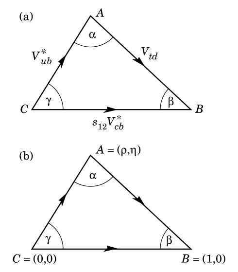
Figure 1: (a) Representation in the complex plane of the triangle formed by the CKM matrix elements $V_{ud}~{}{V_{ub}}^{\!*}$, $V_{td}~{}{V_{tb}}^{\!*}$, and $V_{cd}~{}{V_{cb}}^{\!*}$. (b) Rescaled triangle with vertices A, B, and C at $(\bar{\rho},\bar{\eta)}$, $(1,0)$, and $(0,0)$, respectively.

The angles $\alpha$, $\beta$ and $\gamma$ of the triangle are also referred to as $\phi_{2}$, $\phi_{1}$, and $\phi_{3}$, respectively, with $\beta$ and $\gamma=\delta_{13}$ being the phases of the CKM elements $V_{td}$ and $V_{ub}$ as per

$${V_{td}=|{V_{td}}|e^{-i\beta}},{V_{ub}=|{V_{ub}}|e^{-i\gamma}}~{}.$$ (16)

Rescaling the triangle so that the base is of unit length, the coordinates of the vertices A, B, and C become respectively:

$$\bigl{(}\hbox{Re}(V_{ud}~{}V_{ub}^{\!*})/|V_{cd}~{}V_{cb}^{\!*}|,~{}\hbox{Im}(V_{ud}~{}V_{ub}^{\!*})/|V_{cd}~{}V_{cb}^{\!*}|\bigr{)},~{}(1,0),~{}{\rm and}~{}(0,0)~{}.$$ (17)

The coordinates of the apex of the rescaled unitarity triangle take the simple form $(\bar{\rho},\bar{\eta})$, with $\bar{\rho}=\rho(1-\lambda^{2}/2)$ and $\bar{\eta}=\eta(1-\lambda^{2}/2)$ in the Wolfenstein parametrization, Wolfenstein83 as shown in Figure 1(b).

$CP$-violating processes involve the phase in the CKM matrix, assuming that the observed $CP$ violation is solely related to a nonzero value of this phase. More specifically, a necessary and sufficient condition for $CP$ violation with three generations can be formulated in a parametrization-independent manner in terms of the non-vanishing of $J$, the determinant of the commutator of the mass matrices for the charge $2e/3$ and charge $-e/3$ quarks Jarlskog85 . $CP$-violating amplitudes or differences of rates are all proportional to the product of CKM factors in this quantity, namely $s_{{}_{12}}s_{{}_{13}}s_{{}_{23}}c_{{}_{12}}c_{{}_{13}}^{2}c_{{}_{23}}\sin{\delta_{13}}$. This is just twice the area of the unitarity triangle.

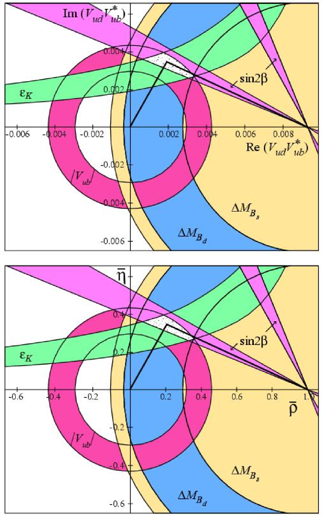
Figure 2: Constraints from the text on the position of the apex, A, of the unitarity triangle following from $|V_{ub}|$,$B$ mixing, $\epsilon$, and $\sin 2\beta$. A possible unitarity triangle is shown with A in the preferred region.

The constraints on the apex of the unitarity triangle that follow from Eqs. (8), (10), (11), (12), and $\epsilon$ are shown in Figure 2. Both the limit on $\Delta M_{s}$ and the value of $\Delta M_{d}$ indicate that the apex lies in the first rather than the second quadrant. All constraints nicely overlap in one small area in the first quadrant with the sign of $\epsilon$ measured in the K system agreeing with the sign of $\sin 2\beta$ measured in the B system. Both the constraints from the lengths of the sides (from $|V_{ub}|$, $|V_{cb}|$, and $|V_{td}|$) and independently those from $CP$-violating processes ($\epsilon$ from the $K$ system and $\sin 2\beta$ from the $B$ system) indicate the same region for the apex of the triangle.

From a combined fit using the direct measurements, B mixing, $\epsilon$, and $\sin 2\beta$, we obtain:

$${\rm Re}~{}V_{td} = 0.0071\pm 0.0008$$ (18)

$${\rm Im}~{}V_{td} = -0.0032\pm 0.0004$$ (19)

$$\bar{\rho} = 0.22\pm 0.10~{},$$ (20)

$$\bar{\eta} = 0.35\pm 0.05~{}.$$ (21)

All processes can be quantitatively understood by one value of the CKM phase $\delta_{{}_{13}}=\gamma=59^{o}\pm 13^{o}$. The value of $\beta=24^{o}\pm 4^{o}$ from the overall fit is consistent with the value from the $CP$ asymmetry measurements of $26^{o}\pm 4^{o}$. The invariant measure of $CP$ violation is $J=(3.0\pm 0.3)\times 10^{-5}$.

*Superallowed $0^{+}\rightarrow 0^{+}$ Beta Decay:
Current Status and Future Prospects
Superallowed $0^{+}\rightarrow 0^{+}$ Beta Decay:
Current Status and Future Prospects J.C. Hardy, I.S. Towner

4 Introduction

Superallowed $0^{+}\rightarrow 0^{+}$ nuclear $\beta$-decay depends uniquely on the vector part of the weak interaction. When it occurs between $T=1$ analog states, a precise measurement of the transition $ft$-value can be used to determine $G_{V}$, the vector coupling constant. This result, in turn, yields $V_{ud}$, the up-down element of the Cabibbo-Kobayashi-Maskawa (CKM) matrix. At this time, it is the key ingredient in one of the most exacting tests available of the unitarity of the CKM matrix, a fundamental pillar of the minimal Standard Model.

5 Current status

Currently, there is a substantial body of precise $ft$-values determined for such transitions and the experimental results are robust, most input data having been obtained from several independent and consistent measurements TH98 ; Ha90 . In all, $ft$-values have been determined for nine $0^{+}\rightarrow 0^{+}$ transitions to a precision of $\sim 0.1\%$ or better. The decay parents – ¹⁰C, ¹⁴O, ^26mAl, ³⁴Cl, ^38mK, ⁴²Sc, ⁴⁶V, ⁵⁰Mn and ⁵⁴Co – span a wide range of nuclear masses; nevertheless, as anticipated by the Conserved Vector Current hypothesis, CVC, all nine yield consistent values for $G_{V}$, from which a value of

$$V_{ud}=0.9740\pm 0.0005$$ (22)

is derived. The unitarity test of the CKM matrix, made possible by this precise value of $V_{ud}$, fails by more than two standard deviations TH98 : viz.

$$V_{ud}^{2}+V_{us}^{2}+V_{ub}^{2}=0.9968\pm 0.0014.$$ (23)

In obtaining this result, we have used the Particle Data Group’s PDG00 recommended values for the much smaller matrix elements, $V_{us}$ and $V_{ub}$. Although this deviation from unitarity is not completely definitive statistically, it is also supported by recent, less precise results from neutron decay Ab02 . If the precision of this test can be improved and it continues to indicate non-unitarity, then the consequences for the Standard Model would be far-reaching.

The potential impact of definitive non-unitarity has led to considerable recent activity, both experimental and theoretical, in the study of superallowed $0^{+}\rightarrow 0^{+}$ transitions, with special attention being focused on the small correction terms that must be applied to the experimental $ft$-values in order to extract $G_{V}$. Specifically, $G_{V}$ is obtained from each $ft$-value via the relationship TH98

$${\cal F}t\equiv ft(1+\delta_{R}^{\prime}+\delta_{NS})(1-\delta_{C})=\frac{K}{2{G_{V}}^{2}(1+\Delta_{\mbox{\tiny R}}^{\mbox{\tiny V}})},$$ (24)

where $K$ is a known constant, $f$ is the statistical rate function and $t$ is the partial half-life for the transition. The correction terms – all of order 1% or less – comprise $\delta_{C}$, the isospin-symmetry-breaking correction, $\delta_{R}^{\prime}$ and $\delta_{NS}$, the transition-dependent parts of the radiative correction and $\Delta_{\mbox{\tiny R}}^{\mbox{\tiny V}}$, the transition-independent part. Here we have also defined ${\cal F}t$ as the “corrected” $ft$-value. Note that, of the four calculated correction terms, two – $\delta_{C}$ and $\delta_{NS}$ – depend on nuclear structure and their influence in Eq.(24) is effectively in the form ($\delta_{C}-\delta_{NS}$).

With Eq.(24) in mind, it is now valuable to dissect the contributions to the uncertainty obtained for $V_{ud}$ in Eq.(22). The contributions to the overall $\pm 0.0005$ uncertainty are 0.0001 from experiment, 0.0001 from $\delta_{R}^{\prime}$, 0.0003 from ($\delta_{C}-\delta_{NS}$), and 0.0004 from $\Delta_{\mbox{\tiny R}}^{\mbox{\tiny V}}$. Thus, if the unitarity test is to be sharpened, then the most pressing objective must be to reduce the uncertainties on $\Delta_{\mbox{\tiny R}}^{\mbox{\tiny V}}$ and ($\delta_{C}-\delta_{NS}$). It is important to recognize that the former also appears in the extraction of $G_{V}$ from neutron decay, and thus it will also ultimately limit the precision achievable from neutron decay to approximately the same level as the current nuclear result, regardless of the precision achieved in the neutron experiments. Improvements in $\Delta_{\mbox{\tiny R}}^{\mbox{\tiny V}}$ are a purely theoretical challenge, the solution of which will not depend on further experiments. However, experiments can play a role in improving the next most important contributor to the uncertainty on $V_{ud}$, namely ($\delta_{C}-\delta_{NS}$). Clearly this correction applies only to the results from superallowed beta decay and, in the event that improvements are made in $\Delta_{\mbox{\tiny R}}^{\mbox{\tiny V}}$, will then limit the precision with which $V_{ud}$ can be determined by this route. Recently, a new set of consistent calculations for ($\delta_{C}-\delta_{NS}$) have appeared TH02 not only for the nine well known superallowed transitions but for eleven other superallowed transitions that are potentially accessible to precise measurements in the future. Experimental activity is now focused on probing these nuclear-structure-dependent corrections with a view to reducing the uncertainty that they introduce into the unitarity test.

6 Future prospects

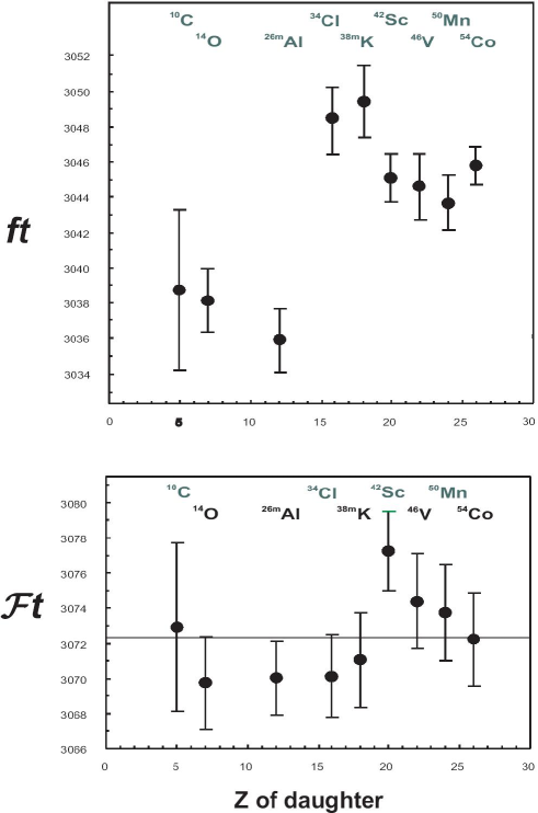
Figure 3: Comparison of experimental ft-values and the corrected ${\cal F}t$-values for the nine well-known superallowed transitions. This illustrates the effect of the calculated nucleus-dependent corrections, which change from transition to transition. (The effect of $\delta_{R}^{\prime}$ is virtually the same for all cases.)

The essential approach being taken by current experiments is best explained with reference to Fig. 3. The upper panel shows the uncorrected experimental $ft$ values and the lower panel the corrected ${\cal F}t$ values with the average indicated by a horizontal line. If the experimental $ft$ values were left uncorrected, their scatter would be quite inconsistent with a single value for the vector coupling constant, $G_{V}$. Once corrected, though, the resulting ${\cal F}t$ values are in excellent agreement with this expectation ($\chi^{2}/\nu=0.6$). This, in itself, provides powerful validation of the calculated corrections used in their derivation. However, extending this concept to measurements of other superallowed decays, we can continue to use CVC to test the validity of the nuclear-structure-dependent corrections, ($\delta_{C}-\delta_{NS}$) at an even more demanding level. By choosing transitions where it is predicted that the structure-dependent corrections are much larger, we can achieve a more sensitive test of the accuracy of the calculations.

Of course it is only the relative values of ($\delta_{C}-\delta_{NS}$) that are confirmed by the absence of transition-to-transition variations in the corrected ${\cal F}t$-values. However, $\delta_{C}$ itself represents a difference – the difference between the parent and daughter-state wave functions caused by charge-dependent mixing. Thus, the experimentally determined variations in $\delta_{C}$ are actually second differences. It would be a pathological fault indeed that could calculate in detail these variations (i.e. second differences) in $\delta_{C}$ while failing to obtain their absolute values (i.e. first differences) to comparable precision.

Experimental attention is currently focused on two series of $0^{+}$ nuclei: the even-$Z$, $T_{z}=-1$ nuclei with $18\leq A\leq 42$, and the odd-$Z$, $T_{z}=0$ nuclei with $A\geq 62$. The main attraction of these new regions is that the calculated values of ($\delta_{C}-\delta_{NS}$) for the superallowed transitions TH02 are larger, or show larger variations from nuclide to nuclide, than the values applied to the nine currently well-known transitions. These are just the properties required to test the accuracy of the calculations. It is argued that if the calculations reproduce the experimentally observed variations where they are large, then that must surely verify their reliability for the original nine transitions whose $\delta_{C}-\delta_{NS}$ values are considerably smaller.

Of the heavier $T_{z}=0$ nuclei, ⁶²Ga and ⁷⁴Rb are receiving the greatest attention at this time (see ref. HT02 and experimental references therein). It is likely, though, that the required experimental precision will take some time to achieve. The decays of nuclei in this series are of higher energy than any previously studied and each therefore involves numerous weak Gamow-Teller transitions in addition to the superallowed transitionHT02 . Branching-ratio measurements are thus very demanding, particularly with the limited intensities likely to be available initially for most of these rather exotic nuclei. In addition, their half-lives are considerably shorter than those of the lighter superallowed emitters; high-precision mass measurements ($\pm 2$ keV) for such short-lived activities will also be very challenging.

More accessible in the short term are the $T_{z}=-1$ superallowed emitters with $18\leq A\leq 42$. There is good reason to explore them. For example, the calculated value of ($\delta_{C}-\delta_{NS}$) for ³⁰S decay, though smaller than those expected for the heavier nuclei, is actually 1.13% – larger than for any other case currently known – while ²²Mg has a low value of 0.51%. Furthermore, the nuclear model space used in the calculation of ($\delta_{C}-\delta_{NS}$) for these nuclei is exactly the same as that used for some of the nine transitions already studied. If the wide range of values predicted for the corrections are confirmed by the measured $ft$-values, then it will do much to increase our confidence (and reduce the uncertainties) in the corrections already being used. To be sure, these decays also provide an experimental challenge, particularly in the measurement of their branching ratios, but sufficiently precise results have just been obtained Ha02 for the half life and superallowed branching ratio for the decay of ²²Mg and work on ³⁴Ar decay is well advanced. New precise $ft$-values should not be long in appearing. It would be virtually impossible for them to have any effect on the central value already obtained for $V_{ud}$ but they may be expected ultimately to lead to reduced uncertainties on that value.

The work of JCH was supported by the U.S. Department of Energy under Grant number DE-FG03-93ER40773 and by the Robert A. Welch Foundation; he would also like to thank the Institute for Nuclear Theory at the University of Washington for its hospitality and support during part of this work.

*New Analysis
of Neutron $\beta$-Decay (Radiative Corrections)
and Implications for CKM Unitarity New Analysis of Neutron $\beta$-Decay (Radiative Corrections)
and Implications for CKM Unitarity W.J. Marciano

7 One and Two Loop Electroweak Corrections

Modulo the Fermi function, electroweak radiative corrections to superallowed $(O^{+}\rightarrow O^{+})$ nuclear beta decays are traditionally factored into two contributions called inner and outer corrections. The outer (or long distance) correction is given by

$$1~{}+~{}\frac{\alpha}{2\pi}(g(E,E_{max})~{}+2C_{NS})~{}+\delta_{2}(Z,E)$$ (25)

where $g(E,E_{max})$ is the universal Sirlin function aso which depends on the nucleus through $E_{max}$, the positron or electron end point energy. $C_{NS}$ is a nuclear structure dependent contribution induced by axial-current nucleon-nucleon interactions itjh and $\delta_{2}$ is an $O(Z\alpha^{2})$ correction partly induced by factorization of the Fermi function and outer radiative corrections wjgr .

The contribution from $g(E,E_{max})$ is quite large $(\sim 1.3\%~{}for~{}O^{14})$ due to a $3\ln(m_{p}/E_{max})$ term which generally dominates. Summation of $(\alpha\ln m_{p}/E_{max})^{n}$, $n=2,3\dots$ contributions from higher orders gives an additional $0.028\%$ correction acwm while additional $O(\alpha^{2})$ effects are estimated to be $<0.01\%$.

$C_{NS}$ and $\delta_{2}(Z,E)$ are nucleus dependent. The leading contribution to $\delta_{2}$ is of the form $Z\alpha^{2}\ln m_{p}/E$ where $Z$ is the charge of the daughter nucleus. Just as in the case of the Fermi function, $\delta_{2}$ is usually given for positron emitters (since that is appropriate for superallowed decays). For electron emitters the sign of $Z$ should be changed in both the Fermi function and $\delta_{2}(Z,E)$. Unfortunately, as pointed out by Czarnecki, Marciano and Sirlin acwm , that sign change was not made in the case of neutron decay. As a result, the often quoted $0.0004$ contribution from $\delta_{2}$ to neutron $\beta$-decay should be changed to $-0.00043$, an overall shift of $-0.083\%$. With those corrections, the overall uncertainty in the outer radiative corrections is now estimated to be about $\pm 0.01\%$.

The inner radiative correction factor is given (at one loop level) by

$$1~{}+~{}\frac{\alpha}{2\pi}(4\ln\frac{m_{Z}}{m_{p}}+\ln\frac{m_{p}}{m_{A}}+A_{g}+2C)$$ (26)

where the $\frac{2\alpha}{\pi}\ln m_{Z}/m_{p}\simeq 0.0213$ universal short- distance correction dominates rmp . The contributions induced by axial- vector effects are relatively small but carry the bulk of the theoretical uncertainty

$$\frac{\alpha}{2\pi}[\ln\frac{m_{p}}{m_{A}}+A_{g}+2C]{\simeq}{-}0.0015\pm 0.0008$$ (27)

It stems from an uncertainty in the effective value of $m_{A}$ that should be employed. The quoted uncertainty in eq. (3) allows for a conservative factor of 2 uncertainty in that quantity. It would be difficult to significantly reduce the uncertainty for nuclei or the neutron. In the case of pion beta decay, the uncertainty is likely to a factor of 2 or more smaller.

High order $(\alpha\ln m_{Z}/m_{p})^{n},n=2,3\dots$ leading log contributions are expected to dominate the multi-loop effects. They have been summed by renormalization group techniques [6], resulting in an increase in eq. (9) by $0.0012$. Next to leading logs of $O(\alpha^{2}\ln m_{Z}/m_{p})$ have been estimated to give $-0.0002\pm 0.0002$ while $O(\alpha^{2})$ effects are expected to be negligible. In total, a recent update finds acwm

$$InnerR.C.Factor=1.0240\pm 0.0008$$ (28)

which is essentially the same as the value given by Sirlin in 1994 lwsi . It leads to

$$|V_{ud}|=0.9740\\ \pm 0.0001\pm 0.0001\pm 0.0003\pm 0.0004$$ (29)

extracted from super-allowed beta decays, where the errors stem from the experimental uncertainty, the two transition dependent parts of the radiative corrections $\delta_{R}^{\prime}$ and $\delta_{C}-\delta_{NS}$, and the inner radiative correction $\Delta_{\mbox{\tiny R}}^{\mbox{\tiny V}}$ respectively.

In the case of neutron decay, the radiative corrections carry a similar structure and uncertainty. Correcting for the sign error in the $Z\alpha^{2}$ effect, one finds the master formula acwm

$$|V_{ud}|^{2}=\frac{4908\pm 4sec}{\tau_{n}(1+3\lambda^{2})}$$ (30)

Employing $\tau_{n}=885.7(7)$s and $\lambda$ = 1.2739(19) then implies

$$|V_{ud}|=0.9717\pm 0.0004\pm 0.0012\pm 0.00004\pm 0.0004$$ (31)

where the errors stems from the experimental uncertainty in the neutron lifetime, the $\beta$-asymmetry $A$ and the theoretical outer and inner radiative correction $\delta_{R}^{\prime}$ and $\Delta_{\mbox{\tiny R}}^{\mbox{\tiny V}}$ respectively. In the case of pion beta decay, the theory uncertainty in $|V_{ud}|$ is probably $\pm 0.0002$ or smaller, but the small $(\simeq 10^{-8})$ branching ratio makes a precision measurement very difficult.

*An Overview of Neutron Decay J. Byrne

8 Neutron Decay in the Context of Nuclear Physics

8.1 The Weak Interaction in Nuclei

According to the Standard Model of particle physics the charged weak current is purely left-handed, i.e. it is an equal admixture of polar vector (V) and axial vector (A) currents of quarks and leptons with appropriate relative sign. In nuclear physics vector currents give rise to Fermi $\beta$ -transitions with coupling constant $G_{V}$ and spin-parity selection rule for allowed transitions:

$$\Delta I=0,\;\textrm{no parity change}$$ (32)

Axial currents give Gamow-Teller $\beta$-transitions with coupling constant $G_{A}$ and spin-parity selection rule for allowed transitions:

$$\Delta I=0,\,\pm 1,\;\textrm{ no }0\Rightarrow 0,\;\textrm{no parity change}$$ (33)

The $\beta$-decay of free neutrons into protons

$$n\Rightarrow p+\;e^{-}+\stackrel{{\scriptstyle\_}}{{\nu}}_{e},\quad\frac{1}{2}^{+}\Rightarrow\frac{1}{2}^{+}$$ (34)

is allowed by both selection rules and is described as a mixed transition. One can therefore observe parity-violating effects in neutron decay associated with vector/axial vector interference.

8.2 Neutron Decay Parameters

The principal kinematic parameters which govern neutron decay are:

$$\Sigma=(m_{n}+m_{p)}c^{2}=1877.83794\,MeV;\Delta=(m_{n}-m_{p})c^{2}=1.29332\,MeV$$ (35)

$$\textrm{Kinetic energy of electrons}:\;0\leq T_{e}\leq 783\,keV$$ (36)

$$\textrm{Kinetic energy of protons}:\;0\leq T_{p}\leq 751\,eV$$ (37)

$$\textrm{Recoil parameter}:\;\delta=\Delta\,/\,\Sigma<10^{-3}$$ (38)

Because the recoil parameter $\delta$ is so small it follows that the momentum transfer dependence of all form factors may be neglected. This is also the reason why the neutron lifetime is so long. The current best value of the neutron lifetime is pdg2 :

$$\tau_{n}=885.7\pm 0.8\,sec.$$ (39)

This is greater by a factor of $\sim 4.10^{8}$ than the lifetime of the muon which is the next longest lived elementary particle.

8.3 Measurement of the Neutron Lifetime

Neutron lifetime experiments may be separated into two groups: the classical ’beam’ methods and the more modern ’bottle’ methods. In beam methods the number of decaying neutrons in a specified volume of neutron beam is recorded. These methods rely on the relationship:

$$\frac{dN(t)}{dt}=-\frac{N(t)}{\tau_{n}}$$ (40)

where N(t) is the number of neutrons in the source volume V at time t. To proceed further we require two additional relations:

$$\Bigl{\langle}\frac{dN(t)}{dt}\Bigr{\rangle}=n_{d}\frac{4\pi}{\Omega\varepsilon}$$ (41)

and

$$\langle N(t)\rangle=\rho_{n}V$$ (42)

where n_d is the number of neutron decays recorded per unit time in a detector of known solid angle $\Omega$ and efficiency $\varepsilon$, and $\rho_{n}$ is the neutron density. Assuming a 4$\pi$ collection solid angle, as in all recent variants of the technique, and unit efficiency $\varepsilon$ for recording the number N_d of decays occurring per second in a known length L of beam, the value of $\tau_{n}$ is given by

$$\tau_{n}=\frac{N_{n}\textrm{ L}}{N_{d}\,\sigma_{0}\,v_{0}\,\eta}$$ (43)

Here N_n is the number of neutron-nucleus reactions detected per unit time in a neutron counter, $\sigma_{0}$ is the cross section at some standard neutron velocity v₀ (usually 2200m./sec.) and $\eta$ is the surface density of neutron detector isotope. This result does not depend on the neutron velocity v, provided $\sigma$(v) scales as v^-1. Suitable reactions are:

$${}^{10}B(n,\alpha)^{7}Li\textrm{ }(\sigma_{0}=3836\pm 8b.),$$ (44)

$${}^{6}Li(n,\alpha)^{3}H\textrm{ }(\sigma_{0}=941\pm 3b.)$$ (45)

and

$${}^{3}He(n,p)^{3}H\textrm{ }(\sigma_{0}=5327\pm 10b.)$$ (46)

’Bottle’ methods for the determination of $\tau_{n}$ on the other hand rely on the integrated form of (40), i.e.

$$N(t)=N(0)\,e^{-t/\tau_{n}}$$ (47)

where N(t) is determined by recording the number of neutrons surviving to time t as a function of the number N(0) present in a fixed source volume at zero time. This is to be contrasted with the beam methods where it is the number of neutrons which fail to survive in a continually replenished source of neutrons which is recorded. Ever since the identification of a storable ultra-cold component of energy $\leq 2.10^{-7}$ eV in the Maxwellian tail of the thermal flux from a reactor, the bottle methods have been favored since they do not rely on the performance of a number of subsidiary experiments,e.g. determination of absolute cross-sections or the precise isotopic composition of neutron counters.

There are two principal neutron storage methods, magnetic confinement or storage in a closed vessel made from a material with suitable Fermi pseudo-potential. Magnetic confinement relies on the force

$$\mathbf{F}=-\nabla\{\mathbf{\mu}_{n}.\mathbf{B}(\mathbf{r})\}$$ (48)

which is exerted on the neutron magnetic moment $\mathbf{\mu}_{n}$ in an inhomogeneous magnetic field $\mathbf{B}(\mathbf{r})$. Since the sense of the force depends on the sign of the spin quantum number only one sign of the spin can be confined which means that, in principle, neutrons can always be lost from the source volume by spin-flipping which is a difficult loss mechanism to control. Alternatively in the case of storage in a material bottle the ideal relation (47) must be replaced by

$$N(t)=N(0)e^{-t(1/\tau_{n}+1/\tau_{w})}$$ (49)

where $\tau_{w}($v$)$ represents the lifetime for neutron loss through absorption or inelastic collisions of ultra-cold neutrons with the walls of the vessel. In general this is given by a relation of the form

$$\tau_{w}(v)^{-1}=\langle\mu(v)\rangle v/\lambda$$ (50)

where $\langle\mu($v$)\rangle$ is the loss rate per bounce averaged over all angles of incidence and the mean free path $\lambda$ is a function of the geometry of the containing vessel. A number of techniques have been developed to estimate $\tau_{w}($v$)$ by using variable geometry and/or counting the number of up-scattered neutrons.

8.4 Neutron Lifetime and the Big Bang

The free neutron lifetime is also of significance in big bang cosmology, where it directly influences the relative abundance of primordial helium synthesized in the early universe. This is determined by the ratio of the neutron lifetime to the expansion time from that epoch at which neutrinos decouple from hadronic matter to the onset of nucleosynthesis schramm .

The argument goes briefly as follows. At times t $<10^{-2}$sec. and temperatures T $>10^{11}$K the populations of neutrons and protons are kept in a state of thermal equilibrium, i.e.

$$X_{n}/X_{p}=e^{-(m_{n}-m_{p})c^{2}/kT}$$ (51)

through the weak interactions

$$n+e^{+}\rightleftharpoons p+\overline{\nu}_{e}\,;\;p+e^{-}\rightleftharpoons n+\nu_{e}$$ (52)

At t $\simeq 1$ sec. the freeze-out temperature T$\simeq 10^{10}$ K is reached where the leptons decouple from the hadrons and neutrons begin to decay into protons according to (34). This process continues until a time t $\simeq 180$ sec when the temperature has fallen to a value T$\simeq$10${}^{9}\,$K and deuterium formed by the capture of neutrons on protons remains stable in the thermal radiation field. This is followed by a sequence of strong interactions whose net effect is the conversion of all free neutrons into helium. Using the current value of the neutron lifetime, these considerations result in a relative helium abundance in the present day universe of about 25% in good agreement with observation.

8.5 Application to Solar Astrophysics

The main source of solar energy derives from the proton-proton cycle of thermonuclear reactions, the end-point of which is the fusion of four protons into a helium nucleus with the release of positrons, photons and neutrinos. In the first step two protons interact weakly to form deuterium

$$p+p\Rightarrow^{2}\!\!\!H+e^{+}+\nu_{e}$$ (53)

An alternative reaction is the weak $p-e-p$ process which occurs with a branching ration of approximately 0.25%

$$p+e^{-}+p\Rightarrow^{2}\!\!\!H+\nu_{e}$$ (54)

That the timescale is determined by the neutron lifetime stems from the fact that the governing reaction (53) is just inverse neutron decay with the spectator proton providing the energy,while the $p-e-p$ interaction (52) is the corresponding electron capture process bahcall . However since the two protons can interact weakly only in the ${}^{1}S_{0}$ state because of the Pauli principle, and since the deuteron can exist only in the triplet state, it follows that the vector contribution to the underlying inverse neutron $\beta$-decay is forbidden and the weak capture of protons on protons proceeds at a rate proportional to ${|}G_{A}|^{2}$. To compute this rate it is therefore necessary to determine individual values for the weak coupling constants $G_{V}$ and $G_{A}$.

8.6 Determination of the Weak Coupling Constants

The neutron lifetime $\tau_{n}=t_{n}/\ln(2)$, where the half-life $t_{n}$ is commonly employed in nuclear physics, is given by the formula

$$ft_{n}=\frac{2\pi^{3}\ln(2)\hbar^{3}}{m_{e}^{5}c^{4}}\cdot[|G_{V\textrm{ }}|^{2}+3|G_{A}|^{2}]^{-1}=\frac{K}{|G_{V\textrm{ }}|^{2}}\cdot[1+3|\lambda|^{2}]^{-1}$$ (55)

where K=(8120.271$\pm 0.012)\cdot 10^{-10}\,$GeV${}^{-4}\,$sec., and

$$\lambda=G_{A}/G_{V\textrm{ }}$$ (56)

The factor f is the integral of the Fermi Coulomb-corrected phase space function $F(E_{e})$ which, including the outer radiative corrections $\delta_{R}>0$, has the value towner

$$f(1+\delta_{R})=1.71489\pm 0.00002$$ (57)

If isospin invariance of the strong interactions and conservation of the weak vector current are assumed, then ${|}G_{V\;}|$ may be determined from the ft-values of the sequence of pure Fermi superallowed 0${}^{+}\Rightarrow 0^{+}$nuclear positron emitters through the formula

$$\overline{ft(1-\delta_{C})(1+\delta_{R})(0^{+}\Rightarrow 0^{+})}=K/|G_{V\textrm{ }}|^{2}$$ (58)

where each nuclear decay has been individually corrected, incorporating factors (1-$\delta_{C})\prec 1$ for isospin symmetry-breaking and (1+$\delta_{R})\succ 1$ for the nucleus-dependent radiative correction. It follows that the values of ${|}G_{V\;}|$ and ${|}G_{A}|$ can be determined from a combination of equations (55) to (58). To determine the relative sign of $G_{V}$ and $G_{A}$ it is necessary to observe some phenomenon which relies on Fermi/Gamow-Teller interference and this requires the availability of polarized neutrons. Such phenomena allow the direct determination $\lambda$ and thus $G_{V}$ and $G_{A}$ can each be determined in both sign and magnitude from neutron decay alone, in which case uncertainties associated with nuclear structure effects do not arise.

9 Neutron Decay in the Context of Particle Physics

9.1 The Cabibbo-Kobayashi-Maskawa Matrix

The neutron and proton form the components of an isospin doublet and are the lightest constituents of the lowest SU(3) flavor octet, each of whose sub-multiplets is characterized by its isospin (I) and its hypercharge (Y). A quantum number alternative to hypercharge is the strangeness S=Y-B where the baryon number B has the value unity. Flavor SU(3) symmetry is based on neglect of the difference in mass between the u- and d-quarks on the one hand, and the s-quark on the other, and is severely broken. Because of the near equality of the u- and d-quark masses the isospin SU(2) symmetry is much more closely realized, a result which is derived from a dynamic global gauge symmetry of the QCD Lagrangian which is expressed in the conservation of the weak vector current.
In increasing order of mass the octet contains an isodoublet {n,p; I=1/2, Y=1}, an isosinglet {$\Lambda^{0};$ I=0, $Y=0\}$, an isotriplet {$\Sigma^{-},\Sigma^{0},\Sigma^{+};$ I=1, $Y=0\}$ and a heavy isodoublet, the so-called cascade particles {$\Xi^{-},\Xi^{0},$ I=1/2, $Y=-1\}$. The $\Sigma^{0}$ decays electromagnetically into the $\Lambda^{0}$ which has the same value of Y and differs only in the value of I which is not conserved by the electromagnetic interaction. Semi-leptonic weak decays within the octet are characterized according to whether they are hypercharge conserving (e.g. $n\Rightarrow p,\Sigma^{-}\Rightarrow\Lambda^{0}$ and $\Sigma^{+}\Rightarrow\Lambda^{0}$), or hypercharge violating (e.g. $\Sigma^{-}\Rightarrow n,\Sigma^{+}\Rightarrow n$ and $\Xi^{-}\Rightarrow\Lambda^{0}).$

It was Cabibbo’s original insight to note and appreciate the significance of the fact that the vector coupling constants corresponding to hypercharge conserving weak decays G${}_{V\textrm{ }}(\Delta Y=0),$and hypercharge non-conserving weak decays G${}_{V\textrm{ }}(\Delta Y=1)$ satisfied the empirical relations

$$G_{V}\,(\Delta Y=0)=G_{F}\cdot\cos(\theta_{c});\;G_{V}\,(\Delta Y=1)=G_{F}\cdot\sin(\theta_{c})$$ (59)

where the Fermi coupling constant $G_{F}$ is determined from the lifetime of the muon and the Cabibbo angle $\theta_{c}\simeq 0.23$. The result (59) is interpreted to mean that the charged vector bosons $W^{\pm}$ which mediate the weak interaction couple to the mixtures of quark mass eigenstates

$$d^{\prime}=d\cdot\cos(\theta_{c})+s\cdot\sin(\theta_{c})\;;\;s^{\prime}=-d\cdot\sin(\theta_{c})+s\cdot\cos(\theta_{c})$$ (60)

rather than to the mass eigenstates of the down ($d$) and strange ($s$) quarks themselves.

In the Standard Model of Particle Physics these ideas are extended to three quark generations where the couplings effective for the weak semi-leptonic decays of quarks are described by the Cabibbo-Kobayashi-Maskawa (CKM) matrix donoghue , which rotates the quark mass eigenstates $(d,s,b)$ to the weak eigenstates$(d^{{}^{\prime}},s^{{}^{\prime}},b^{{}^{\prime}})$:

$$\left(\begin{array}[]{c}d^{{}^{\prime}}\\ s^{{}^{\prime}}\\ b^{\prime}\end{array}\right)=\left(\begin{array}[]{ccc}V_{ud}&V_{us}&V_{ub}\\ V_{cd}&V_{cs}&V_{cb}\\ V_{td}&V_{ts}&V_{tb}\end{array}\right)\left(\begin{array}[]{c}d\\ s\\ b\end{array}\right)$$ (61)

where

$$V_{ud}\simeq V_{cs}\simeq\cos(\theta_{c})\;;\;V_{us}\simeq-V_{cd}\simeq\sin(\theta_{c})$$ (62)

Since, assuming that no more than three quark generations exist, the CKM matrix must be unitary, its nine elements can be expressed in terms of only four real parameters, three of which can be chosen as real angles and the fourth as a phase. If this phase is not an integral multiple of $\pi$, then CP symmetry is violated. For this to be possible the number of quark generations must be at least three. In the present context the unitarity of the CKM matrix requires that

$$|V_{ud}|^{2}+|V_{us}|^{2}+|V_{ub}|^{2}=1$$ (63)

and the role of neutron $\beta$-decay centers on the determination of the largest matrix element $V_{ud}$.

9.2 Neutron Decay in the Standard Model

In the Standard Model the weak interaction responsible for neutron decay is given as the contraction of a leptonic current $J_{\mu}^{l}(x)$ and a hadronic current $J_{\mu}^{h}(x)$, where, in the convention that the operator (1-$\gamma_{5})/2$ projects out the left-handed field components,

$$J_{\mu}^{l}(x)=\overline{e}\gamma_{\mu}(1-\gamma_{5})\nu_{e\;};\;J_{\mu}^{h}(x)=\overline{d}\cdot V_{ud}\gamma_{\mu}(1-\gamma_{5})u_{\;}$$ (64)

Since the leptons have no strong interactions the matrix element of the weak leptonic current is relatively simple, i.e.

$$\langle e^{-}\overline{\nu}_{e}|J_{\mu}^{l}(0)|0\rangle=\langle\overline{u_{e}}|\gamma_{\mu}(1-\gamma_{5})|u_{\nu_{e}}\rangle$$ (65)

where u_e and u${}_{\nu_{e}}$ are Dirac spinors describing electron and neutrino respectively. However since the quarks are strongly interacting particles confined in nucleons the hadronic matrix elements are in principle limited only by the requirements of Lorentz invariance and maximal parity violation. Thus we find for the matrix element of the vector current

$$\langle p|J_{\mu}^{h,V}(0)|n\rangle=\langle\overline{v_{p}}|g_{V}(q)\gamma_{\mu}-i\frac{\hbar}{2m_{p}c}g_{WM}(q)\sigma_{\mu\nu}q_{\nu}+\frac{\hbar}{2m_{p}c}g_{S}(q)q_{\mu}|v_{n}\rangle$$ (66)

where $v_{n}$ and $v_{p}$ are neutron and proton spinors respectively, q_μ is the 4-momentum transfer and g${}_{i}(i=V,$ $WM,$ $S)$ represent form factors corresponding to the bare vector, induced weak magnetism and induced scalar interactions respectively. As noted in section 8.2, for neutron decay all form factors may be evaluated at $q=0$. Conservation of the vector current then requires that

$$g_{V}(0)=1,\quad g_{WM}(0)=\kappa_{p}-\kappa_{n}=3.70,\quad g_{S}(0)=0.$$ (67)

where $\kappa_{p}=1.79,$and $\kappa_{n}=-1.91,$ are the anomalous magnetic moments of neutron and proton respectively, expressed in units of the nuclear magneton. Since weak magnetism is a term of recoil order it makes only a very small correction to the vector matrix element in neutron decay and is totally absent in pure Fermi decays. An alternative test of the conserved weak vector current theorem in action outside the regime of baryon decays is the pure Fermi 0${}^{-}\Rightarrow 0^{-}$ $\beta$-decay $\pi^{+}\Rightarrow\pi^{0}+e^{+}+\nu_{e}$. The induced scalar interaction is also ruled out on the separate grounds that, having the wrong transformation properties under the G-parity transformation, it is second class and therefore does not contribute to $\beta-$decays within an isospin multiplet holstein .

The corresponding axial matrix element is

$$\left\langle p\;|J_{\mu}^{h,A}(0)|n\right\rangle=\left\langle\overline{v_{p}}|g_{A}(q)\gamma_{\mu}\gamma_{5}-i\frac{\hbar}{2m_{p}c}g_{T}(q)\sigma_{\mu\nu}q_{\nu}\gamma_{5}+\frac{\hbar}{2m_{p}c}g_{P}(q)q_{\mu}\gamma_{5}|v_{n}\right\rangle$$ (68)

The axial current is not conserved which means that the form factor $g_{A}(0)$ is nucleon structure dependent and has to be determined experimentally. Since the induced tensor form factor g${}_{T}(0)$ is also ruled out as second class, and the operator $q_{\mu}\gamma_{5}$ does not contribute to allowed decay between nuclear states of the same parity, it follows that the axial matrix element depends only on the single constant $g_{A}(0)$ which, given that $g_{V}(0)=1,$ becomes identical with the empirical constant $\lambda$ introduced in (54).

10 The Correlation Coefficients in Neutron Decay

10.1 Polarized Neutron Decay

In a pure Fermi transition nuclear polarization is not possible and in a pure Gamow-Teller transition only the M=$\pm 1$ lepton magnetic substates contribute to the correlation between the nuclear spin and the lepton momenta. This is the origin of the parity violation phenomenon first observed in the decay of ${}^{60}Co$. However, in a mixed transition such as in neutron decay, interference can arise between the singlet and triplet magnetic substates with M=0. As a consequence, depending on the sign of $\lambda$, either the electron or the antineutrino asymmetry will be enhanced as compared with pure Gamow-Teller decay, the other being reduced in proportion.

Experimental study of the angular and polarization coefficients which characterizes the decay of unpolarized and polarized neutrons offers an alternative route to the determination of $\lambda$. These involve carrying out measurements of the neutron spin polarization $\mathbf{\sigma}_{n},$ and perhaps the electron polarization $\mathbf{\sigma}_{e},$ together with some combination of the energies $E_{e},E_{\bar{\nu}},E_{p}$ and momenta $\mathbf{p}_{e},\mathbf{p}_{\bar{\nu}}$, $\mathbf{p}_{p}$ of the three particles in the final state. The transition rate for a polarized neutron can then be written jackson :

$$dW(\mathbf{\sigma},\mathbf{p}_{e},\mathbf{p}_{\bar{\nu}})\propto F(E_{e})d\Omega_{e}d\Omega_{\bar{\nu}}\{1+a\,\frac{\mathbf{p}_{e}\,\mathbf{.\,p}_{\bar{\nu}}}{E_{e}E_{\bar{\nu}}}+\frac{bm_{e}}{E_{e}}+$$

$$+\langle\mathbf{\sigma}_{n}\mathbf{\rangle(}A\frac{\mathbf{p}_{e}}{E_{e}}+B\frac{\mathbf{p}_{\bar{\nu}}}{E_{\bar{\nu}}}+D\frac{\mathbf{p}_{e}\,\times\,\mathbf{p}_{\bar{\nu}}}{E_{e}E_{\bar{\nu}}}\mathbf{+}R\frac{\,\mathbf{\sigma}_{e}\,\times\,\mathbf{p}_{e}\,}{E_{e}}+\ldots)\}$$ (69)

where the neutron polarization $\mathbf{\sigma}_{n}$ has been averaged over all wavelengths and positions within the neutron beam and some less significant correlations have been omitted. The three correlation coefficients $a,A$ and $B$, which have finite values within the Standard Model, are given in lowest order by the relations:

$$a=\frac{1-|\lambda|^{2}}{1+3|\lambda|^{2}},\quad A=-2\frac{|\lambda|^{2}+\mathit{Re}(\lambda)}{1+3|\lambda|^{2}},\quad B=2\frac{|\lambda|^{2}-\mathit{Re}(\lambda)}{1+3|\lambda|^{2}}$$ (70)

where the possibility has been left open that the coupling constant ratio $\lambda$ might be complex signalling a break-down of time reversal invariance in the weak interaction. Each of these coefficients has to be corrected by inclusion of radiative corrections plus additional terms of recoil order including weak magnetism. However certain linear combinations of these coefficients exist which are independent of radiative corrections to lowest order in the fine structure constant $\alpha$ omitting cross terms of order $\alpha q$ or $\alpha(E_{e}/m_{p})\ln(m_{p}/E_{e})$. These relations are garcia :

$$f_{1}=1+A-B-a=0;\quad f_{2}=aB-A^{2}--A=0$$ (71)

The possibility of a breakdown in T-invariance is tested in a measurement of the T-odd, P-even triple correlation coefficient D which is given by the expression

$$D=\frac{2\mathit{Im}(\lambda)}{1+3|\lambda|^{2}}$$ (72)

In order to establish a violation of T-invariance it is necessary to identify some feature of the decay which changes sign under reversal of the time but not under inversion of the coordinate system. The term $\mathbf{\sigma}_{n}\,\cdot(\mathbf{p}_{e}\times\,\mathbf{p}_{\bar{\nu}})$ possesses the desired property.

10.2 Non-Standard Model Contributions to the Correlation Coefficients

The leading coefficients $a,A$ and $B$ are each sensitive to right-handed contributions to the weak interaction irrespective of any possible contribution from scalar or tensor couplings. For example in left-right symmetric models the coefficient A takes the formcarnoy

$$A=-2\frac{|\lambda|^{2}(1+y^{2})+\mathit{Re}(\lambda)(1-xy)+T_{1}}{1+x^{2}+3|\lambda|^{2}(1+y^{2})+T_{2}}$$ (73)

where T₁and T₂ are small terms of recoil order, x $\simeq\delta-\zeta,$ $y\simeq\delta+\zeta,\delta$ is the square of the ratio of the mass of the light W-boson which couples to left-handed currents to the mass of the postulated heavy W-boson coupling to right handed currents and $\zeta$ is the mixing angle. In these models D is linear in $\zeta$ and is particularly sensitive to a T-violating coupling of a left-handed lepton to a right-handed quark.

When the possibility is allowed for contributions from scalar and tensor couplings then both the Fierz interference coefficient $b$ and the T-violating coefficient $R$ receive finite contributions. Specifically

$$b=b_{F}+b_{GT}\propto\mathit{Re}(G_{V}G_{S}^{*}+G_{V}^{\prime}G_{S}^{\prime\,*})-3\mathit{Re}(G_{A}G_{T}^{*}+G_{A}^{\prime}G_{T}^{\prime\,*})$$ (74)

and

$$R=R_{F}+R_{GT}\propto-\mathit{Im}(G_{A}^{\prime}G_{S}^{*}+G_{A}G_{S}^{\,*})+$$

$$+\mathit{Im}(3Re(G_{A}G_{T}^{*}+G_{A}^{\prime}G_{T}^{\prime\,*})+G_{V}^{\prime}G_{T}^{*}+G_{V}G_{T}^{\prime\,*})$$ (75)

where in this case it is necessary quite generally to distinguish between coupling constants which are P-conserving (e.g. $G_{V}$) and P-non-conserving (e.g. $G_{V}^{\prime}$). The Fermi coefficients b_F and R_F are particularly sensitive to the scalar coupling of a right-handed lepton to any quark while the Gamow-Teller coefficients are sensitive to the tensor coupling of a right-handed lepton to a left-handed quark deutsch .

11 Measurement of the Correlation Coefficients

11.1 The Electron-Antineutrino Angular Correlation Coefficient $a$

Since the electron spectrum in allowed $\beta$-decay is determined by the Fermi phase space factor F(E${}_{e})$ alone, it is insensitive to the details of the weak interaction. Thus, up to the discovery of parity violation, the correlation coefficient $a$ was the only parameter available to provide such information. Also since the operator p${}_{e\,}.\mathbf{p}_{\bar{\nu}}$ commutes with the total angular momentum of the leptons, and therefore does not mix singlet and triplet operators, it follows that the correlation coefficient

$$a=\frac{1-|\lambda|^{2}}{1+3|\lambda|^{2}};\qquad\frac{\delta|\lambda|}{|\lambda|}\simeq 0.27\frac{\delta a}{a}\simeq 1\%$$ (76)

contains no Fermi/Gamow-Teller interference terms apart from small terms of recoil order.

It is, of course, impracticable to measure the correlation between the electron and antineutrino momenta directly, since efficient detectors of antineutrinos do not exist. In practice therefore only two indirect methods have been have been employed. These are (a) measuring the momentum spectrum of electrons emitted into a given range of angles referred to the proton momentum and (b) measuring the proton spectrum nachti . The experimenter is therefore presented with a choice between electron spectroscopy and proton spectroscopy and both methods have been explored…

It turns out that, up to the present, the measurement of the proton spectrum has proved the more fruitful and two studies of this nature have been completed. These have used (a) proton magnetic spectroscopy and (b) a Penning trap with adiabatic focusing.Both experiments have required the addition of post acceleration of the protons to energies of order 20-30 keV and have each reached precisions on $a$ at the level of 5%. Because this correlation measures the anomaly in ${|}\lambda|$ rather than ${|}\lambda|$ itself the resultant error in ${|}\lambda|$ is reduced to $\simeq$1.4%.

Angular correlation measurements have the great advantage that it is not necessary that the neutrons be polarized and this route to the determination of ${|}\lambda|$ has yet to achieve its true potential.

11.2 The Electron-Neutron Spin Asymmetry Coefficient $A$

The correlation coefficient

$$A=-2\frac{|\lambda|^{2}+\mathit{Re}(\lambda)}{1+3|\lambda|^{2}};\qquad\frac{\delta\lambda|}{\lambda}\simeq 0.24\frac{\delta A}{A}\simeq 0.23\%$$ (77)

has been subjected to an enormous amount of experimental study going back to the 1950’s. It has provided the most precise value for the parameter $\lambda$ both in magnitude and sign, and therefore for the CKM matrix element V_ud based on neutron decay alone hartmut . This information has been largely derived from studies over the past $\simeq$15 years at the ILL, Grenoble using the electron spectrometer PERKEO in its various forms. The current world average value for $\lambda$ is pdg2 :

$$\lambda=-1.2670\pm 0.0030\$$ (78)

Like the $a$-coefficient, the $A$-coefficient has the great advantage the it measures the anomaly in $\lambda$. However it relies critically on $\simeq$1 MeV electron spectroscopy, and, although this is in general easier to perform than $\simeq$ 1 keV proton spectroscopy, it has not proved possible to extend the electron spectrum down to the lowest energies. However the measurement of $A$ suffers from the great disadvantage that the neutrons must be polarized and the neutron polarization must be measured to an accuracy $\geq 99\%$ and this is not easy. Fortunately discrepancies between the values of the polarization derived using polarizer/analyser combinations based on supermirrors and ${}^{3}He$ filters appear to have been satisfactorily resolved.

11.3 The Antineutrino-Neutron Spin Asymmetry Coefficient B

The correlation

$$B=2\frac{|\lambda|^{2}-\mathit{Re}(\lambda)}{1+3|\lambda|^{2}};\qquad\frac{\delta\lambda}{\lambda}\simeq 2.0\frac{\delta B}{B}$$ (79)

is quite insensitive to the value of $\lambda$. Its measurement has the disadvantages that it requires both that the neutrons be polarized and that proton spectroscopy be performed. For both these reasons it has tended to be neglected as a topic for study. However, for the same reason that it is insensitive to the precise value of $\lambda$, it is very sensitive to contributions from right-handed bosons and recent measurements have succeeded in setting a limit $m_{BR}>284.3\,GeV/c^{2}$ for the mass of the heavy W-boson which is postulated to couple to right-handed currents serebrov .

A recent encouraging development has been the simultaneous measurement of $A$ and $B$ whose ratio is therefore independent of neutron polarization 14 .

11.4 The Triple Correlation Coefficient D

This coefficient

$$D=\frac{2\mathit{Im}(\lambda)}{1+3|\lambda|^{2}}$$ (80)

is measured by counting coincidences between electrons and protons detected in counters set at appropriately selected angles for a given sign of the neutron spin. The spin is then reversed and the relevant counting rate asymmetry is recorded.

The D-coefficient is of second order in the T-violating phase in the CKM matrix and is expected to be vanishingly small. Currently it is known to vanish at a level of about 0.1% from neutron decay, and to marginally better precision from the decay of ${}^{19}Ne$. However, since the T-symmetry is non-unitary and is generated by a non-linear operator, a violation can be mimicked by final state electromagnetic interactions which in this instance appear at a level of about 0.001%.

12 Additional Experimental Possibilities

12.1 The Proton-Neutron Spin Asymmetry Coefficient $\alpha$

The individual coefficients A and B each have terms in ${|}\lambda|^{2}$ deriving from the axial vector interaction, in addition to terms in Re($\lambda)$ generated through polar vector/axial vector interference. Suppose, instead, one were to measure the correlation $\alpha\mathbf{\sigma}_{n}\cdot\mathbf{p}_{p}$ by detecting the complete range of proton energies but without recording electron coincidences. Then, since this is a parity-violating term and no lepton is detected, it satisfies the conditions of Weinberg’s interference theorem 15 , and is therefore proportional to Re($\lambda)$ with no term in ${|}\lambda|^{2}$. The corresponding expression for the coefficient $\alpha$ is given by 16 :

$$\alpha=C\frac{4\lambda}{1+3|\lambda|^{2}},\qquad C=0.27484,\qquad\frac{\delta\lambda}{\lambda}\simeq 1.5\frac{\delta\alpha}{\alpha}$$ (81)

where the kinematic constant C comes from the double integral over electron and proton energies, and includes Coulomb, recoil order and radiative corrections. Since in lowest order the correlation $\alpha$ is proportional to (A+B) it is also relatively insensitive to the value of $\lambda$.

The principle of an experiment is quite straightforward. Recoil protons from the decay of longitudinally polarized neutrons are collected in a magnetic field of order 5T, where the maximum radius of the cyclotron orbit is $\prec 1mm$. If $N^{+}(N^{-})$ denote the numbers of protons with momenta parallel (anti-parallel) to the neutron spin, then $N^{\pm}=N_{0}\{1\pm\alpha\langle\mathbf{\sigma}_{n}\rangle/2\}$ and the appropriate counting rate asymmetry can be computed.

To measure $N^{\pm}$, $s$et the orientation of the neutron spin parallel to the magnetic field and reflect the protons from a $\simeq$1kV electrostatic potential barrier so that protons of both senses of momentum enter the detector which is maintained at about $-30\,kV$. Thus the counting rate is given by

$$C_{1}=N^{+}+N^{-}+b$$ (82)

where $b$ is the background. When the reflecting potential barrier is removed the new counting rate is

$$C_{2}=N^{+}+\beta N^{-}+b$$ (83)

where $\beta\ll 1$ represents that fraction of protons initially moving away from the detector which is reflected back into the detector by magnetic mirror action. The procedure is now repeated with the neutron spin direction reversed giving corresponding counting rates $C_{1}^{{}^{\prime}},C_{2}^{{}^{\prime}}$ and background $b^{\prime}$. The counting rate asymmetry is then given by

$$\frac{(C_{1}^{{}^{\prime}}-C_{2}^{{}^{\prime}})-(C_{1}-C_{2})}{(C_{1}^{{}^{\prime}}-C_{2}^{{}^{\prime}})+(C_{1}-C_{2})}=\alpha\langle\mathbf{\sigma}_{n}\rangle$$ (84)

The experiment only works on the assumption that the proton counter background in the energy range $\leq 30\,keV$ is weak in comparison to the signal strength which is certainly not true in the case that the neutrons are polarized using a supermirror.

12.2 Two-Body Decay of the Neutron and Right-Handed Currents

When a neutron undergoes $\beta-$decay there is a small branching ratio $\simeq$4.10^-6 that the final state should contain an antineutrino and a hydrogen atom i.e.

$$n\Rightarrow H+\stackrel{{\scriptstyle\_}}{{\nu}}_{e},$$ (85)

where the hydrogen atom is created in an S-state. Since this is a two-body decay, momentum conservation ensures that antineutrino and hydrogen atom each carry off unique energies with

$$\mathbf{p}_{\bar{\nu}}+\mathbf{p}_{H}=0,\qquad E_{\bar{\nu}}=783\,keV,\qquad T_{H}=352\,eV$$ (86)

Although the higher S-levels decay spontaneously, hydrogen atoms created in the metastable 2S state can exist in one of four decoupled hyperfine levels $|M_{e},M_{p}\rangle$ with populations W${}_{i}(i=1-4)$, where $\mathbf{n}_{H}=\mathbf{p}_{H}/p_{H}$ and

$$\left|\frac{1}{2},\frac{1}{2}\right\rangle;\quad\;\;\;W_{1}=2(1+|\lambda|^{2})\{1+\mathbf{\sigma}_{n}\mathbf{.n}_{H}\}\simeq 0.57\%\quad\mathrm{when}\quad\mathbf{\sigma}_{n}\mathbf{.n}_{H}=0$$ (87)

$$\left|-\frac{1}{2},\frac{1}{2}\right\rangle;\quad W_{2}=8|\lambda|^{2}\{1-\mathbf{\sigma}_{n}\mathbf{.n}_{H}\}\simeq 55.13\%\quad\mathrm{when}\quad\mathbf{\sigma}_{n}\mathbf{.n}_{H}=0$$ (88)

$$\left|\frac{1}{2},-\frac{1}{2}\right\rangle;\quad W_{3}=2(1-|\lambda|^{2})\{1-\mathbf{\sigma}_{n}\mathbf{.n}_{H}\}\simeq 44.28\%\quad\mathrm{when}\quad\mathbf{\sigma}_{n}\mathbf{.n}_{H}=0$$ (89)

$$\left|-\frac{1}{2},-\frac{1}{2}\right\rangle;\;W_{4}=2(1+|\lambda|^{2})\{1+\mathbf{\sigma}_{n}\mathbf{.}\stackrel{{\scriptstyle}}{{\mathbf{n}}}_{H}\}\equiv 0$$ (90)

The population $W_{4}$ vanishes identically in the case that the weak interaction is purely left-handed, and this is a result which depends on conservation of angular momentum only. Thus exploiting the neutron polarization to suppress the populations $W_{2}$ and $W_{3}$, observation of a finite population $W_{4}$ $\neq 0$ would provide an unambiguous signature for the existence of right-handed currents 17 .

12.3 Radiative Neutron Decay

Radiative decay of the free neutron

$$n\Rightarrow p+\;e^{-}+\stackrel{{\scriptstyle\_}}{{\nu}}_{e}+\gamma,$$ (91)

also described as inner bremsstrahlung, has a branching ratio at the level of 0.1%. The matrix element for the process consists of two terms; a term describing electron photon emission and a term describing proton photon emission. Both terms contain infra-red divergences which cancel. However because ${|}\lambda|\neq 1$, contrary to the situation in the case of the muon which has no strong interactions, the total radiative correction depends on the ultra-violet cut-off parameter $\Lambda$. Thus the simplest experiments designed to detect the inner bremsstrahlung provide a measure of the outer radiative correction only.

Experiments designed to measure the branching ratio for radiative neutron decay by detecting triple coincidences between electron, proton and gamma are currently under way at the ILL Grenoble 18 .

*Neutron Lifetime Value
Measured by Storing Ultra-Cold Neutrons with Detection of Inelastically Scattered Neutrons

Neutron Lifetime Value Measured by Storing Ultra-Cold Neutrons with Detection of Inelastically Scattered Neutrons

S. Arzumanov, L. Bondarenko, W. Drexel, A. Fomin, P. Geltenbort,
V. Morozov, Yu. Panin, J. Pendlebury, K. Schreckenbach S. Arzumanov, L. Bondarenko, Chernyavsky, W. Drexel, A. Fomin,
P. Geltenbort, V. Morozov, Yu. Panin, J. Pendlebury, K. Schreckenbach

13 Introduction

A detailed description of this experiment was published in Arzu . In a simple quark picture of the free neutron beta decay a $d$ quark transforms into an $u$ quark under emission of a virtual $W$-boson which in turn decays into an electron and an electron antineutrino. A breakthrough in precision of the neutron lifetime has been achieved by storage experiments of ultra cold neutrons 1 ; 2 ; 3 . Including results from the correlation coefficients between the decay partners, in particular the beta asymmetry coefficient A 4 ; 5 ; 6 the vector and axial vector coupling constants $g_{V}$ and $g_{A}$ were deduced from the neutron decay alone. The obtained value for $g_{V}$ was compared with data from muon decay and superallowed beta-decays yielding stringent limits on possible deviations from the universality of the weak interaction coupling constants, on right handed currents and on the unitarity of the CKM matrix 4 ; 7 ; 8 .

In neutron lifetime measurements by UCN storage the UCN’s are contained by material walls due to the Fermi-pseudo potential, by gravity or by the interaction on the neutron’s magnetic moment with a magnetic field gradient. Conceptually those experiments are quite simple. UCN’s are filled in a storage volume with suitable walls. After a storage period the surviving neutrons are counted. Repeating this experiment with different storage times yields the decay curve of the neutrons. The major problem encountered in this method is caused by losses of UCN in collisions with the trap walls. Extrapolation to infinite trap size yielded $\tau_{n}=1/\lambda_{n}$.

In the present experiment new method was used to separate wall losses from beta decay. The main loss process was monitored during storage by measuring the relative flux of inelastically scattered UCN by a set of neutron detectors surrounding the vessel, see Fig.1. The survival probability of the UCN was measured by the usual UCN storage and disappearance method of the neutrons in the trap. The trap was arranged such that the UCN could be stored in two different sections with different surface to volume ratios and hence different total UCN survival times. Comparing the survival time and upscattering rates for the two volumes yielded the value of $\tau_{n}$.

14 Basic idea of the experimental method

When monoenergetic UCN are in the trap, the number of neutrons $N(t)$ in the trap changes exponentially during the storage time, i.e. $N(t)=N_{0}e^{-\lambda t}$. The value $\lambda$ is the total probability per unit time for the disappearance of UCN due to both the beta-decay and losses during UCN-wall collisions. In turn, losses are equal to the sum of the inelastic scattering rate constant $\lambda_{ie},$ and that for the neutron capture at the wall, $\lambda_{cap}$.

$$\lambda=\lambda_{n}+\lambda_{loss}=\lambda_{n}+\lambda_{ie}+\lambda_{cap}$$ (92)

The ratio $\lambda_{cap}/\lambda_{ie}$ is to a good approximation equal to the ratio of the UCN capture and inelastic scattering cross sections for the material of the wall surface since both values are proportional to the wall reflection rate of UCN in the trap:

$$a=\lambda_{loss}/\lambda_{ie}=1+\lambda_{cap}/\lambda_{ie}=1+\sigma_{cap}/\sigma_{ie}$$ (93)

and is constant for the given conditions, i.e. same wall material and temperature. During storage the upscattered neutrons are recorded with an efficiency $\varepsilon_{th}$ in the thermal neutron detector surrounding the storage trap. The total counts in the time interval $T$ is equal to

$$J=\varepsilon_{th}\lambda_{ie}\left(N_{0}-N_{T}\right)/\lambda$$ (94)

Here $N_{0}$ and $N_{T}$ are the UCN populations in the trap at the beginning and the end of the storage time $T$, respectively. The UCN themselves are measured with an efficiency $\varepsilon$ such that the detected UCN at the beginning (normalization measurement) and the end of the storage time are equal to $N_{i}=\varepsilon N_{0}$ and $N_{f}=\varepsilon N_{T}$ respectively. We have then :

$$\lambda_{ie}=\frac{J\lambda}{\left(N_{i}-N_{f}\right)}\frac{\varepsilon}{\varepsilon_{th}}$$ (95)

and

$$\lambda=\frac{1}{T}\ln(N_{i}/N_{f})$$ (96)

The experiment is repeated with a different value for the wall loss rates with constant value $a$. Thus $\lambda_{n}$ is given by

$$\lambda_{n}=\frac{\xi\lambda^{(1)}-\lambda^{(2)}}{\xi-1}$$ (97)

where

$$\xi=\lambda_{ie}^{(2)}/\lambda_{ie}^{(1)}$$ (98)

The indices refer to the two measurements with different $\lambda_{loss}$. The result contains then only the ratios of the directly measured quantities $J,N_{i},N_{f}$ since the efficiencies of the neutron detection cancel. It is very important that this method is thus relative and asks only the time interval absolute measurement.

15 Method for a broad UCN energy spectrum

In a real experiment it is necessary to take into account the energy distribution of UCN since the scattering and capture cross sections are in general energy dependent and losses are different for different parts of the UCN energy spectrum. It makes the measurement more complex. Nevertheless, the main idea - the relativity of the experiment, remains the same. In this case the result evaluation includes $\lambda$-values, averaged over the storage period $T$ ($\bar{\lambda}_{ie}$, $\bar{\lambda}$), as well as new parameters (ratios $\varepsilon_{i}/\varepsilon_{f}$, coefficients $k$ in the time function for $\lambda_{ie}$etc) which were measured during the storage period or at additional experiments. The ratio ${\varepsilon_{th}^{(1)}}/{\varepsilon_{th}^{(2)}}$ of the thermal neutron detection was calculated by the Monte Carlo method that was evaluated by the Monte-Carlo method using the neutron cross sections measured at special experiments for neutrons that were inelastically scattered during storing time.

Now the UCN populations decay at different rates in the trap 9 and:

$$N(t)=N_{0}\exp\left(\int\limits_{0}^{t}-\lambda(t^{\prime})dt^{\prime}\right)$$ (99)

The rate $\lambda(t)=\lambda_{n}+\lambda_{loss}(t)\$ and $\lambda_{ie}(t)=\lambda_{ie0}(1-\gamma t)$. The quantity $\gamma$ is order of $10^{-{\bf 4}}s^{-1}$ when $T\ll 1/\lambda_{loss}$.

Using the above parameter definition we have $\lambda_{loss}=\lambda_{ie}(t)\cdot a$ and the mean value of $\lambda(t)$ over the time interval $T$ is then given by

$$\bar{\lambda}=1/T\int\lambda(t)dt=\lambda_{n}+\lambda_{ie0}(1-\frac{\gamma T}{2})a\ \hskip 72.26999pt$$ (100)

and

$$\bar{\lambda}=\frac{1}{T}ln(\frac{N_{i}}{N_{f}}\cdot\frac{\varepsilon_{f}}{\varepsilon_{i}})$$ (101)

where the ratio of the UCN detection efficiency $\varepsilon_{i}$, $\varepsilon_{f}$ varies slightly with $T$. The value of $a$ in the case where trap walls are coated by a layer of hydrogenfree oil (Fomblin type) is close to unity: $a-1<2\cdot 10^{-2}$ and temperature dependent.

The full counts of the thermal neutron detector during storage is equal to

$$J=\varepsilon_{th}\lambda_{ie0}N_{0}\cdot\int_{0}^{T}(1-\gamma t)\exp[-\left(\bar{\lambda}+\lambda_{ie0}a\gamma(T-t)/2\right)t]dt$$ (102)

Expanding the second part of the exponent, neglecting the $\gamma^{2}$ terms and solving for $\lambda_{ie0}$ gives

$$\lambda_{ie0}=\frac{\bar{\lambda}J}{(N_{i}-N_{f})\Phi}\cdot\frac{\varepsilon}{\varepsilon_{th}}$$ (103)

where

$$\Phi=1-\frac{\gamma}{\bar{\lambda}}(1+\frac{1}{2}\lambda_{ie0}aT)I_{2}/I_{1}+\frac{1}{2}\lambda_{ie0}\frac{\gamma a}{\bar{\lambda}^{2}}I_{3}/I_{1}$$ (104)

and $I_{1}=\int_{0}^{\bar{\lambda}T}e^{-x}dx$; $I_{2}=\int_{0}^{\bar{\lambda}T}e^{-x}xdx$; $I_{3}=\int_{0}^{\bar{\lambda}T}e^{-x}x^{2}dx$.

The measured value

$$\bar{\lambda}_{ie}=\frac{J\bar{\lambda}}{(N_{i}-N_{f})}\cdot\frac{\varepsilon}{\varepsilon_{th}}$$ (105)

and performing the pair of measurements with two different loss rate values, the $\lambda_{n}$ value is derived as

$$\lambda_{n}=\frac{\xi\bar{\lambda}^{(1)}-\bar{\lambda}^{(2)}}{\xi-1}$$ (106)

where the $\xi$-value is determined by:

$$\xi=\frac{\bar{\lambda}_{ie}^{(2)}}{\bar{\lambda}_{ie}^{(1)}}\cdot\frac{\left(1-\frac{\gamma^{(2)}T^{(2)}}{2}\right)\Phi^{(1)}a^{(2)}}{\left(1-\frac{\gamma^{(1)}T^{(1)}}{2}\right)\Phi^{(2)}a^{(1)}}$$ (107)

The correction terms relative to the monoenergetic case are quite small if cleaning times $(t_{cl}^{(1),(2)},$ see next section$)$ are chosen properly to have almost the same stored UCN spectra. In addition the product $\gamma T$ is constant to a good approximation, when storage times are scaled such that the same average number of wall reflections occur in $T$. The deviation of $\Phi$ and $a$ from unity are in the percent range, if the specification of the wall (temperature, type of wall, etc.) is the same, and depend only on the surface to volume ratio via the development of the UCN spectrum during storage. The values for $\Phi$ and $a$ can be determined in particular from the time dependence $j(t)$ of the upscattering rate during the storage time.

The UCN detection efficiency $\varepsilon$ includes also the UCN losses in the vessel during the emptying time of the vessel into the UCN detector. To take into account a slight change of $\varepsilon$, the counting rate $n(t)$ of the UCN detector during the emptying phase has to be corrected for the decay rate $\bar{\lambda}$.

16 The experiment

The experiment was carried out at the UCN source of the ILL High Flux Reactor in Grenoble.

The storage vessel was composed of two coaxial horizontal cylinders which walls were coated with a thin layer of Fomblin. The storage vessel was placed inside the vacuum housing which had the cooling system stabilized the bottle temperature in the range $+20^{\circ}$C to $-26^{\circ}$C. Residual gas pressure in the storage vessel was about $(1\div 5)\cdot 10^{-6}$ torr. The set-up was surrounded by the thermal neutron detectors and supplied with the UCN detector, both ³He filled. The whole installation was placed inside the shielding: Cd of 1mm thick and boron polyethylene of 16cm thick.

The UCN were stored either in the inner cylinder or in the annular gap between both cylinders thereby changing the UCN loss rate by a factor of about 4 without breaking the vacuum. The construction allowed to refresh the oil layers on the cylinder walls also without a vacuum break.

In the experiment there were measured counting rates of both detectors: $j(t)$, $n(t)$ during storage time interval $T$ as well as integral counts$\ J,N_{i},N_{f}.$ The elementary run consisted of two consequent measurements with the UCN storage in both vessels. These elementary runs were repeated as many times as was necessary to get sufficient statistics.

As discussed above the storage time intervals $T^{(1)},T^{(2)}$ in the inner vessel (⁽¹⁾) and the annular vessel (⁽²⁾) as well as $t_{cl}^{(1)},t_{cl}^{(2)}$ were chosen to make almost the same evolution of the UCN spectra.

Groups of experimental runs were performed at the different temperature $+20$, $-8$, $-9$ and $-26$ ^∘C, respectively.

17 Evaluation of the data and result

A data evaluation was performed on the base of the method developed for a spread UCN spectrum. Some important details of calculations:

1. The parameter $a$ was constant for a run at the same wall temperature as the temperature of the vessel was stabilized and constant over the wall surface within 0.1^∘C (for room temperature) and 1.5^∘C (for the lower temperatures).

2. An important correction for $\tau_{n}$ of $-3.10\pm 0.36$s arose from the ratios of the UCN detection efficiencies $\varepsilon^{(1)}/\varepsilon^{(2)}$ and $\varepsilon_{f}/\varepsilon_{i}$.These ratios were experimentally determined from the counting rates $n(t)$ combined with measured values for $\bar{\lambda}$.

3. The ratio $\varepsilon_{th}^{(1)}/\varepsilon_{th}^{(2)}$ of the thermal neutron detection was calculated by the Monte Carlo method using mean values for the capture and scattering cross sections (also measured in special experiments) for neutrons that were inelastically scattered during the storing time. The correction in $\tau_{n}$ was $0.6\pm 0.3$s. The systematic error in this calculation reflects the uncertainty of the geometry, the upscattering cross sections and the spectrum of upscattered neutrons.

4. Time distributions $j(t)$ were used to determine the $k$-parameter for $\bar{\lambda}_{ie}$ and the $\xi$-values. Compared to a monoenergetic UCN spectrum the correction in $\tau_{n}$ was $-2.0\pm 0.3$s.

5. Since the different bottle temperatures lead to very different loss rates, the consistency of the set of neutron life time values with divergence of error bar, obtained for the different bottle temperatures, gives confidence in the experimental method used.

6. The final result: $\tau_{n}$[sec]=885.4$\pm$ 0.9(stat)$\pm$ 0.4(system).

7. The uncertainties in $\tau_{n}$ due to the ratios $\varepsilon^{(1)}/\varepsilon^{(2)}(0.36$s) and $\varepsilon_{f}/\varepsilon_{i}(0.3$s) as well as due to $k(0.3$s) are included in the statistical error since they are based on the measured time spectra of detectors counting rates.

8. The possible systematic error for $\tau_{n}$ is composed of

   1. the uncertainty in $\varepsilon_{th}^{(1)}/\varepsilon_{th}^{(2)}$ $(0.3$s),

   2. the influence of the UCN scattering at the residual gas $(0.2$s),

   3. the epi-Fomblin neutron impurity in the UCN spectrum $(0.2$s)

   4. the temperature difference over the walls $(0.15$s),

   and was estimated (added up in quadrature) as $0.4$s.

   The present experimental result is in agreement with the recent evaluation of earlier data on the neutron life time of 886.7(1.9)s by the Particle Data Group. New one (PDG-2001) is equal to 885.7(0.8)s

18 Conclusion

1. Presented method of the neutron lifetime measurement is relative and does not demand the absolute calibrations of the apparatus except of the timer.

2. The most part of the necessary parameters (the UCN detection efficiencies, the UCN spectrum change rates etc) were measured during the storage experiment. The other parameters were specially measured under the storage experiment conditions.

3. Monte Carlo evaluation of the ratio of the detection efficiencies for thermal neutrons was based on these measured parameters.

4. The final result changed the world mean value on one second and, seems, concluded the precision possibility of our method.

19 Acknowledgments

The authors like to express their deep gratitude to S.T.Belyaev for his interest and fruitful discussions and support of this investigation. We are pleased to thank Dr.P.Iaydjiev for his help and cooperation during the long period of measurements at the UCN source of the ILL. Authors are grateful to Prof.A.Steyerl and Dr.E.Korobkina for attentive discussions and fruitful criticisms of the presentation. The experiment could not have been carried out without the intensive and very skilful assistance of H.Just to whom we would like to express our thanks. The authors like to thank very much the ILL reactor personnel for much help and informal assistance.

This experiment was made possible due to supports of INTAS (grant 93-298) and of Russian Foundation for Basic Research (grant RFBR 93-02-3927).

*Is the Unitarity of the
Quark-Mixing CKM Matrix
Violated in Neutron $\beta$-Decay?
Is the Unitarity of the Quark-Mixing CKM Matrix Violated in Neutron $\beta$-Decay? H. Abele

20 The Standard Model, Quark-Mixing and the CKM Matrix

This article is about the interplay between the Standard Model of elementary particle physics and neutron $\beta$-decay. Since the Fermi decay constant is known from muon decay, the Standard Model describes neutron $\beta$-decay with only two additional parameters. One parameter is the first entry $|V_{ud}|$ of the CKM matrix. The other one is $\lambda$, the ratio of the vector coupling constant and the axial vector constant. In principle, the ratio $\lambda$ can be determined from QCD lattice gauge theory calculation, but the results of the best calculations vary by up to 30%. In neutron decay, several observables are accessible to experiment, which depend on these parameters, so the problem is overdetermined and, together with other data from particle and nuclear physics, many tests of the Standard Model become possible. The chosen observables for determining $|V_{ud}|$ are the neutron lifetime $\tau$ and a measurement of the $\beta$-asymmetry parameter $A_{0}$.

As is well known, the quark eigenstates of the weak interaction do not correspond to the quark mass eigenstates. The weak eigenstates are related to the mass eigenstates in terms of a 3 x 3 unitary matrix $V$, the so called Cabibbo-Kobayashi-Maskawa (CKM) matrix. By convention, the u, c and t quarks are unmixed and all mixing is expressed via the CKM matrix ${\it V}$ operating on d, s and b quarks. The values of individual matrix elements are determined from weak decays of the relevant quarks. Unitarity requires that the sum of the squares of the matrix elements for each row and column be unity. So far precision tests of unitarity have been possible for the first row of ${\it V}$, namely

$$|V_{ud}|^{2}+|V_{us}|^{2}+|V_{ub}|^{2}=1-\Delta$$ (108)

In the Standard Model, the CKM matrix is unitary with $\Delta$ = 0.

A violation of unitarity in the first row of the CKM matrix is a challenge to the three generation Standard Model. The data available so far do not preclude there being more than three generations; CKM matrix entries deduced from unitarity might be altered when the CKM matrix is expanded to accommodate more generations Groom ; Marciano1 . A deviation $\Delta$ has been related to concepts beyond the Standard Model, such as couplings to exotic fermions Langacker1 ; Maalampi , to the existence of an additional Z boson Langacker2 ; Marciano2 or to the existence of right-handed currents in the weak interaction Deutsch . A non-unitarity of the CKM matrix in models with an extended quark sector give rise to an induced neutron electric dipol moment that can be within reach of next generation of experiments Liao .

Due to its large size, a determination of $|V_{ud}|$ is most important. It has been derived from a series of experiments on superallowed nuclear $\beta$-decay through determination of phase space and measurements of partial lifetimes. With the inclusion of nuclear structure effect corretions a value of $|V_{ud}|$ = 0.9740(5) Hardy emerges in good agreement of different, independent measurements in nine nuclei. Combined with $|V_{us}|$ = 0.2196(23) from kaon-decays and $|V_{ub}|$ = 0.0036(9) from B-decays, this lead to $\Delta$ = 0.0032(14), signaling a deviation from the Unitarity condition by 2.3 $\sigma$ standard deviation. The quoted uncertainty in $|V_{ud}|$, however, is dominated by theory due to amount, size and complexity of theoretical uncertainties. Although the radiative corretions include effects of order Z$\alpha^{2}$, part of the nuclear corrections are difficult to calculate. Further, the change in charge-symmetry-violation for quarks inside nuclei results in an additional change in the predicted decay rate which might lead to a systematic underestimate of $|V_{ud}|$. A limit has been reached where new concepts are needed to progress. Such are offered by studies with neutron and with limitations with pion $\beta$-decay. The pion $\beta$-decay has been measured recently at the PSI. The pion has a different hadron structure compared with neutron or nucleons and it offers an other possibility in determining $|V_{ud}|$. The preliminary result is $|V_{ud}|$=0.9771(56) Pocanic . The somewhat large error is due to the small branching ratio of 10^-8.

Further information on the CKM matrix and the unitarity triangle are based on a workshop held at CERN Battaglia and a workshop held at Heidelberg HADM .

21 Neutron-$\beta$-Decay

In this article, we derive $|V_{ud}|$, not from nuclear $\beta$-decay, but from neutron decay data. In this way, the unitarity check of (1) is based solely on particle data, i.e. neutron $\beta$-decay, K-decays, and B-decays, where theoretical uncertainties are significantly smaller. So much progress has been made using highly polarized cold neutron beams with an improved detector setup that we are now capable of competing with nuclear $\beta$-decays in extracting a value for $V_{ud}$, whilst avoiding the problems linked to nuclear structure.

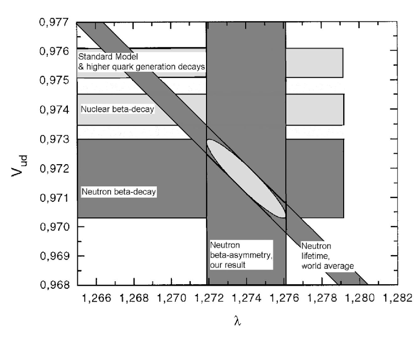
Figure 4: $|V_{ud}|$ vs. $\lambda$. $|V_{ud}|$ was derived from $Ft$ values of nuclear $\beta$-decays, higher quark generation decays, assuming the unitarity of the CKM matrix, and neutron $\beta$-decay.

A neutron decays into a proton, an electron and an electron antineutrino. Observables are the neutron lifetime $\tau$ and spins $\sigma_{e}$, $\sigma_{\nu}$, $\sigma_{p}$, and momenta $p_{e}$, $p_{\nu}$, $p_{p}$ of the electron, antineutrino and proton respectively. The electron spin, the proton spin and the antineutrino are not usually observed. The lifetime is given by

$$\tau^{-1}=C|V_{ud}|^{2}(1+3\lambda^{2})f^{R}(1+\Delta_{R}),$$ (109)

where $C=G_{F}^{2}m_{e}^{5}/(2\pi^{3})=1.1613\cdot 10^{-4}s^{-1}$ in $\hbar=c=1$ units, $f^{R}$ =1.71335(15) is the phase space factor (including the model independent radiative correction) adjusted for the current value of the neutron-proton transition energy and corrected by Marciano MarcianoHA . $\Delta_{R}$ = 0.0240(8) is the model dependent radiative correction to the neutron decay rate Towner1 . The $\beta$-asymmetry $A_{0}$ is linked to the probability that an electron is emitted with angle $\vartheta$ with respect to the neutron spin polarization $P$ = $<\sigma_{z}>$:

$$W(\vartheta)=1+\frac{v}{c}PA\cos(\vartheta),$$ (110)

where $v/c$ is the electron velocity expressed in fractions of the speed of light. ${\it A}$ is the $\beta$-asymmetry coefficient which depends on $\lambda$. On account of order 1% corrections for weak magnetism, $g_{V}-g_{A}$ interference, and nucleon recoil, ${\it A}$ has the form $A$ = $A_{0}$(1+$A_{{\mu}m}$($A_{1}W_{0}+A_{2}W+A_{3}/W$)) with electron total energy $W=E_{e}/m_{e}c^{2}+1$ (endpoint $W_{0}$). $A_{0}$ is a function of $\lambda$

$$A_{0}=-2\frac{\lambda(\lambda+1)}{1+3\lambda^{2}},$$ (111)

where we have assumed that $\lambda$ is real. The coefficients $A_{{\mu}m}$, $A_{1}$, $A_{2}$, $A_{3}$ are from Wilkinson1 taking a different $\lambda$ convention into consideration. In addition, a further small radiative correction Gluck of order 0.1% must be applied. For comparison, information about $|V_{ud}|$ and $\lambda$ are shown in Fig. (1). The bands represent the one sigma error of the measurements. The $\beta$-aymmetry $A_{0}$ in neutron decay depends only on $\lambda$, while the neutron lifetime $\tau$ depends both on $\lambda$ and $|V_{ud}|$. The intersection between the curve, derived from $\tau$ and $A_{0}$, defines $|V_{ud}|$ within one standard deviation, which is indicated by the error ellipse. Other information on $|V_{ud}|$, derived from nuclear $\beta$-decay and higher quark generation decays are shown, too. As can be seen from Fig. (1), both the nuclear $\beta$-decay result from Hardy and the neutron $\beta$-decay from Abele2 do not agree with this unitarity value.

22 The Experiment PERKEO and the Result for $|V_{ud}|$

The following section is about our measurement of the neutron $\beta$-asymmetry coefficient $A$ with the instrument PERKEOII, and on the consequences for $|V_{ud}|$. The strategy of PERKEOII followed the instrument PERKEO Bopp in minimizing background and maximizing signal with a $4\pi$ solid angle acceptance over a large region of the beam. Major achievements of the instrument PERKEO are:

• The signal to background ratio in the range of interest is 200.

• The overall correction of the raw data is 2.04%.

• The detector design allows an energy calibration with linearity better than 1%.

• New polarizers and developments in polarization analysis led to smaller uncertainties related to neutron beam polarization.

Figure 5: A schematic view of the whole setup at the ILL.

For a measurement of $\beta$-asymmetry $A_{0}$, the instrument PERKEO was installed at the PF1 cold neutron beam position at the High Flux Reactor at the Institut Laue-Langevin, Grenoble. Cold neutrons are obtained from a 25 K deuterium cold moderator near the core of the 57 MW uranium reactor. The neutrons are guided via a 60 m long neutron guide of cross section 6 $\times$ 12 cm² to the experiment and are polarized by a 3 $\times$ 4.5 cm² supermirror polarizer. The de Broglie wavelength spectrum of the cold neutron beam ranges from about 0.2 nm to 1.3 nm. The degree of neutron polarization was measured to be P = 98.9(3)% over the full cross section of the beam. The polarization efficiency remained constant during the whole experiment. The neutron polarization is reversed periodically with a current sheet spin flipper. The main component of the PERKEO II spectrometer is a superconducting 1.1 T magnet in a split pair configuration, with a coil diameter of about one meter. Neutrons pass through the spectrometer, whereas decay electrons are guided by the magnetic field to either one of two scintillation detectors with photomultiplier readout. The detector solid angle of acceptance is truly 2$\times$2$\pi$ above a threshold of 60 keV. Electron backscattering effects, serious sources of systematic error in $\beta$-spectroscopy, are effectively suppressed. Technical details about the instrument can be found in Abele ; Reich . The measured electron spectra $N^{\uparrow}_{i}(E_{e})$ and $N^{\downarrow}_{i}(E_{e})$ in the two detectors (i=1,2) for neutron spin up and down, respectively, define the experimental asymmetry as a function of electron kinetic energy $E_{e}$ and are shown in Fig. 3.

$$A_{i_{exp}}(E_{e})=\frac{N^{\uparrow}_{i}(E_{e})-N^{\downarrow}_{i}(E_{e})}{N^{\uparrow}_{i}(E_{e})+N^{\downarrow}_{i}(E_{e})}.$$ (112)

By using (3) and with $<\cos(\vartheta)>$ = 1/2, $A_{i}{{}_{exp}}(E)$ is directly related to the asymmetry parameter

$$A_{exp}(E_{e})=A_{1_{exp}}(E_{e})-A_{2_{exp}}(E_{e})=\frac{v}{c}APf.$$ (113)

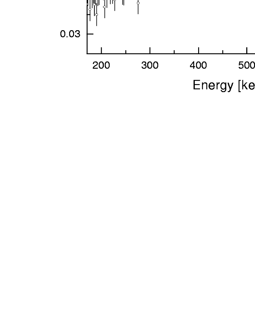
Figure 6: Fit to the experimental asymmetry $A_{exp}$ for detector 1 and detector 2. The solid line shows the fit interval, whereas the dotted line shows an extrapolation to higher and lower energies.

The experimental function $A_{i_{exp}}(E_{e})$ and a fit with one free parameter $A_{i_{exp}}$ (the absolute scale of $A_{0}$) is shown in Fig. 6. The total correction for the small experimental systematic effects is 2.04%.

With recent experiments from the University of Heidelberg Abele2 ; Abele , we obtain $A_{0}$ = -0.1189(7) and $\lambda$ = - 1.2739(19). With this value, and the world average for $\tau$ = 885.7(7) s, we find that $|V_{ud}|$ = 0.9717(13). With $|V_{us}|$ = 0.2196(23) and the negligibly small $|V_{ub}|$ = 0.0036(9), one gets

$$|V_{ud}|^{2}+|V_{us}|^{2}+|V_{ub}|^{2}=1-\Delta=0.9924(28).$$ (114)

This value differs from the Standard Model prediction by $\Delta$ = 0.0076(28), or 2.7 times the stated error. Earlier experiments Bopp ; Yerozolimsky ; Schreckenbach gave significant lower values for $\lambda$. Averaging over our new result and previous results, the Particle Data Group Groom arrives at a new world average for $|V_{ud}|$ from neutron $\beta$-decay which leads to a 2.2 s deviation from unitarity.

An independent test of CKM unitarity comes from W physics at LEP Sbarra where W decay hadronic branching ratios can be used. Since decay into the top quark channel is forbidden by energy conservation one would expect $\sum{|V_{ij}|^{2}}$ to be 2 with a three generation unitary CKM matrix. The experimental result is 2.032(32), consistent with (7) but with considerably lower accuracy.

23 The future

The main corrections in the experiment PERKEO are due to neutron beam polarization (1.1%), background (0.5%) and flipper efficiency (0.3%). The total correction is 2.04%. With such small corrections to the data, we start to see a deviation from the Standard Model already in the uncorrected raw data. For the future, the plan is further to reduce all corrections. In the meantime, major improvements both in neutron flux and degree of neutron polarization has been made: First, the new ballistic supermirror guide at the ILL from the University of Heidelberg gives an increase of a factor of 4 in the cold neutron flux Haese1 . Second, a new arrangement of two supermirror polarizers allows to achieve an unprecedented degree of neutron polarization $P$ of between 99.5% and 100% over the full cross section of the beam Soldner1 . Third, systematic limitations of polarization measurements have been investigated: The beam polarization can now be measured with a completely new method using an opaque ³He spin filter with an uncertainty of 0.1% Heil ; Zimmerha . As a consequence, we are now in the lucky situation to improve on the main uncertainties in reducing the main correction of 1.1% to less than 0.5% with an error of 0.1%. Thus, a possible deviation from the Standard Model, if confirmed, will be seen very pronounced in the uncorrected data.

24 Summary

$|V_{ud}|$, the first element of the CKM matrix, has been derived from neutron decay experiments in such a way that a unitarity test of the CKM matrix can be performed based solely on particle physics data. With this value, we find a 2.7 $\sigma$ standard deviation from unitarity, which conflicts the prediction of the Standard Model of particle physics.

Future trends have been presented on this workshop ”Quark-mixing, CKM Unitarity” in Heidelberg. Regarding the Unitarity problem, about half a dozen new instruments are planed or under construction to allow for beta-neutrino correlation $a$ and $\beta$-asymmetry $A$ measurements at the sub-10^-3 level. With next generation experiments measurements with a decay rate of over 10⁵s^-1 become feasible Dubbers3 .

*CKM Unitarity and $|\rm V_{cs}|$ from W Decays CKM Unitarity and $|\rm V_{cs}|$ from W Decays E. Barberio

25 Introduction

Within the framework of the Standard Model of electroweak interactions, the elements of the Cabibbo-Kobayashi-Maskawa (CKM) ckm mixing matrix are free parameters, constrained only by the requirement that the matrix be unitary. The values of the matrix elements can only be determined by experiment.

In general, CKM elements are derived from the measurement of weak hadronic decays. Since quarks are bound in hadrons QCD symmetries need to be employed to parameterize the non-perturbative aspects of QCD. Hence, for most of these elements the principal error is no longer experimental but rather theoretical: it reflects theoretical models and the assumption invoked.

In the Standard Model the branching fraction of the W boson decays depend on the six CKM matrix elements which do not involve the top quark. Measuring the W production rates for different flavors gives access to the individual CKM matrix elements without parameterization of non-perturbative QCD:

$$\Gamma(\rm W\to q^{\prime}\bar{q})=\frac{C(\alpha_{s})G_{F}M^{3}_{W}}{6\sqrt{2\pi}}|V_{ij}|^{2}=(707\pm 1)|V_{ij}|^{2}\rm MeV$$

where

$$C(\alpha_{s})=3\bigg{[}1+\sum_{i=1,3}\frac{a_{i}\alpha_{s}(\rm{M}^{2}_{\rm{W}})}{\pi}\bigg{]}$$

is the QCD color factor, up to the third order in $\alpha_{s}(\rm{M}^{2}_{\rm{W}})$, the strong coupling constant.

Furthermore, ’on shell’ W bosons decay before the hadronization process starts, and the quark transition occurs in a perturbative QCD regime. Hence, W boson decays offer a complementary way to determine the CKM matrix elements.

From 1997 to 2000 the LEP $\rm e^{+}e^{-}$collider has been operated at energies above the threshold for W-pair production. This offered a unique opportunity to study the hadronic decays of W boson in a clean environment and to investigate the coupling strength of W boson bosons to different quark flavors.

26 $|V_{\rm{cs}}|$ from hadron decays

Values of $|V_{\rm{cs}}|$ can be obtained from neutrino scattering production of charm and form semileptonic D decays with theoretical uncertainties larger than 10%. The value of $|V_{\rm{cs}}|$ extracted from neutrino scattering production of charm depends on assumption about the s-quark sea density in partons. This method gives a lower bound of 0.59.

Using semileptonic D decays one measures:

$${\rm\Gamma(D\to Ke\nu)=}|f^{D}_{+}(0)|^{2}\rm~{}|V_{\rm{cs}}|^{2}~{}(1.54\cdot 10^{11})~{}s^{-1},$$

where $|f^{D}_{+}(0)|$ is the D_e3 form factor. The most recent evaluation of the magnitude of $|V_{\rm{cs}}|$ from this method yields $|V_{\rm{cs}}|=1.04\pm 0.16$ pdgbarber , dominated by theoretical uncertainties which exceed 10%.

27 $|V_{\rm{cs}}|$ from W decays

Each one of the four LEP experiment collected a data sample of about 15000 W-pair events. This sample is not large enough to measure a the six CKM elements not involving the top quark, but large enough to improve the knowledge of the matrix element $|V_{\rm{cs}}|$. This was the least well known CKM element. It is of order one, while the production of bottom quarks is in fact highly suppressed due to the small magnitude of $|V_{\rm{ub}}|$ and $|V_{\rm{cb}}|$ and the large mass of the top quark, the weak partner of the bottom quark. The same data set can be used to test unitarity of the first two rows of the CKM matrix at the few percent level.

Using W decays, the magnitude of the CKM matrix element $|V_{\rm{cs}}|$ can be derived indirectly from either the W boson leptonic branching fraction or the a direct measurement of the production fraction of charm in W decays. $|V_{\rm{cs}}|$ can then be derived from the charm production rate or the W boson leptonic branching fraction, using the knowledge of the other CKM matrix elements. A direct measurement can be done from the direct measurement of the $\rm W\to cs$ transition.

The indirect measurement provides a high statistical sample and use the fact that so far direct measurements of $|V_{\rm{cs}}|$ have limited precision compared to the other CKM matrix elements important in W boson decays, i.e. $|V_{\rm{ud}}|$, $|V_{\rm{us}}|$, and $|V_{\rm{cd}}|$.

The direct observation of the $\rm W\to cs$ transition requires either very good particle identification or a large WW sample (much larger than the LEP one).

Experimentally quarks from W decays form jets and to measure all six CKM elements the original flavor of the quark which originated the jet needs to be identified. This is possible, due to the strong correlation between the primary quark flavor and the jet properties.

The identification of charm or the beauty quarks is relatively easy. Their tagging is based on well understood and unambiguous special properties: long lifetime, higher jet multiplicity, etc. The identification of light quark (u-,d-, s-quark) to a precision needed for a meaningful measurement of the CKM elements is more difficult and requires large statistics and/or good particle identification.

The observation of $\rm W\to cx$ transition requires the identification of a charm jet. The observation of $\rm W\to cs$ transition requires the identification of a charm jet and a strange jet.

27.1 $|V_{\rm{cs}}|$ from charm production rate

At LEP the production rate of charm in W bosons can be measured without a separation of charm and bottom quarks decays. Charm hadron identification is based upon jet properties in particular on lifetime information and semileptonic decay products in the events. The measured value of $R_{\rm{c}}^{\rm{W}}$is then used to determine $|V_{\rm{cs}}|$.

$$R_{\rm{c}}^{\rm{W}}=\frac{\Gamma\rm(W\to c\,X)}{\Gamma\,(W\to hadrons)}=\frac{|V_{\rm{cd}}|^{2}+|V_{\rm{cs}}|^{2}+|V_{\rm{cb}}|^{2}}{|V_{\rm{ud}}|^{2}+|V_{\rm{us}}|^{2}+|V_{\rm{ub}}|^{2}+|V_{\rm{cd}}|^{2}+|V_{\rm{cs}}|^{2}+|V_{\rm{cb}}|^{2}}.$$

In the Standard Model $R_{\rm{c}}^{\rm{W}}=0.5$, due to the CKM unitarity.

Charm jets are identified using a multi-dimensional estimator based on charm jet characteristics: the most powerful discriminator are the lifetime information and leptons produced in charm decays. Weakly decaying charm hadrons have lifetimes between 0.2 ps and 1 ps pdgbarber , leading to typical decay lengths of a few hundred microns to a few millimeters at LEP2 energies. These relatively long–lived particles produce secondary decay vertices which are significantly displaced from the primary event vertex. About $20\,\%$ of all charm hadrons decay semi-leptonically and produce an electron or a muon in the final state. Because of the relatively large mass and hard fragmentation of the charm quark compared to light quarks, this lepton is expected to have a larger momentum than leptons from other sources (except the small contribution from semileptonic bottom decays in background events). Therefore, identified electrons and muons can be used as tags for charm hadrons in W boson boson decays.

Three LEP collaborations rcwaleph , rcwdelphi and rcwopal measured $R_{\rm{c}}^{\rm{W}}$using only a part of their data set. Their average gives:

$$R_{\rm{c}}^{\rm{W}}=0.49\pm 0.03_{stat}\pm 0.03_{sys},$$

where the systematics error is dominated by the Monte Carlo calibration of the analysis. This result is consistent with the Standard Model prediction that the $\rm{W}$ boson couples to up and charm quarks with equal strength. There is no much gain in using the full LEP W-pairs data set for this method as the total error is limited by systematics errors correlated between the LEP experiments.

Using direct measurements of the other CKM matrix elements and $\Gamma^{W}_{tot}=2.135\pm 0.069$ GeV mass , $|V_{\rm{cs}}|$ can be calculated from $R_{\rm{c}}^{\rm{W}}$:

$$|V_{\rm{cs}}|=\rm\frac{R_{\rm{c}}^{\rm{W}}Br(W\to had)\Gamma^{W}_{tot}}{(701\pm 1)\rm MeV}$$

yielding $|V_{\rm{cs}}|=0.976\pm 0.88_{R_{\rm{c}}^{\rm{W}}}\pm 0.003_{CKM}$.

27.2 $|V_{\rm{cs}}|$ from W leptonic branching fraction

This method provide the most precise determination of $|V_{\rm{cs}}|$ and is the one which provided the smallest error.

The leptonic branching fraction of the W boson $\mathcal{B}(\mbox{$\rm{W}\rightarrow\ell\overline{\nu}_{\ell}$})$ is related to the six CKM elements not involving the top quark by:

$$\frac{1}{\mathcal{B}(\mbox{$\rm{W}\rightarrow\ell\overline{\nu}_{\ell}$})}\quad=\quad C(\alpha_{s}(\rm{M}^{2}_{\rm{W}}))\sum_{\tiny\begin{array}[]{c}i=(u,c),\\ j=(d,s,b)\\ \end{array}}|\rm{V}_{ij}|^{2}.$$

Using $\alpha_{s}(\rm{M}^{2}_{\rm{W}})$=$0.121\pm 0.002$, the measured leptonic branching fraction of the W yields

$$\sum_{\tiny\begin{array}[]{c}i=(u,c),\\ j=(d,s,b)\\ \end{array}}|\rm{V}_{ij}|^{2}\quad=\quad 2.039\,\pm\,0.025_{{\cal{B}}(Wtolnu)}\pm\,0.001_{\alpha_{s}},$$ (115)

where the first error is due to the uncertainty on the branching fraction measurement and the second to the uncertainty on $\alpha_{s}$ lep . This result is consistent with the unitarity of the first two rows of the CKM matrix at the 1.5% level, as in the Standard Model:

$$\sum_{\tiny\begin{array}[]{c}i=(u,c),\\ j=(d,s,b)\\ \end{array}}|\rm{V}_{ij}|^{2}=2.$$ (116)

No assumption on the values of the single CKM elements are made.

Using the experimental knowledge pdgbarber of the sum $|\rm{V}_{ud}|^{2}+|\rm{V}_{us}|^{2}+|\rm{V}_{ub}|^{2}+|\rm{V}_{cd}|^{2}+|\rm{V}_{cb}|^{2}=1.0477\pm 0.0074$, the above result can also be interpreted as a measurement of $|\rm{V}_{cs}|$:

$$|\rm{V}_{cs}|\quad=\quad 0.996\,\pm\,0.013.$$

The error includes a $\pm 0.0006$ contribution from the uncertainty on $\alpha_{s}$ and a $\pm 0.004$ contribution from the uncertainties on the other CKM matrix elements, the largest of which is that on $|\rm{V}_{cd}|$. These contributions are negligible compared to the experimental error from the measurement of the W branching fractions, $\pm 0.013$.

The W decay branching fractions, $\mathcal{B}(\rm{W}\rightarrow\textrm{f}\overline{\textrm{f}}^{\prime})$, are determined from the cross sections for the individual WW$\rightarrow\rm{4f}$ decay channels measured by the four experiments at all energies above 161 GeV. These branching fractions can be derived with and without the assumption of lepton universality. In the fit with lepton universality, the branching fraction to hadrons is determined from that to leptons by constraining the sum to unity.

Results from the experiments lep and the LEP combined values are given in Table 1. Figure 7 shows the results of the LEP combination.

Table 1: Summary of leptonic and hadronic W branching fractions derived from preliminary W-pair production cross sections measurements up to 207 GeV centre–of–mass energy.

	Lepton			Lepton
	non–universality			universality
Experiment	B($\rm{W}\rightarrow\rm{e\overline{\nu}_{e}}$)	B($\rm{W}\rightarrow\mu\overline{\nu}_{\mu}$)	B($\rm{W}\rightarrow\tau\overline{\nu}_{\tau}$)	B($\rm{W}\rightarrow\rm{hadrons}$)
	[%]	[%]	[%]	[%]
Aleph	$10.95\pm 0.31$	$11.11\pm 0.29$	$10.57\pm 0.38$	$67.33\pm 0.47$
Delphi	$10.36\pm 0.34$	$10.62\pm 0.28$	$10.99\pm 0.47$	$68.10\pm 0.52$
L3	$10.40\pm 0.30$	$\phantom{0}9.72\pm 0.31$	$11.78\pm 0.43$	$68.34\pm 0.52$
Opal	$10.40\pm 0.35$	$10.61\pm 0.35$	$11.18\pm 0.48$	$67.91\pm 0.61$
LEP	$10.54\pm 0.17$	$10.54\pm 0.16$	$11.09\pm 0.22$	$67.92\pm 0.27$
$\chi^{2}/\textrm{d.o.f.}$	14.9/9			18.8/11

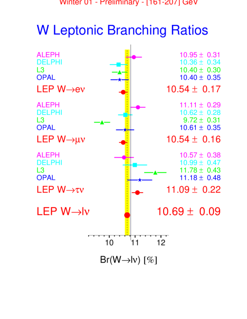
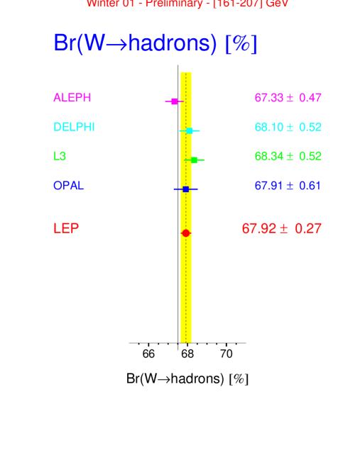
Figure 7: Summary of leptonic and hadronic W branching fractions derived from preliminary W-pair production cross sections measurements up to 207 GeV centre–of–mass energy.

Assuming lepton universality, the measured hadronic branching fraction is $67.92\pm 0.17\rm{(stat.)}\pm 0.21\rm{(syst.)}\%$ and the measured leptonic branching fraction is $10.69\pm 0.06\rm{(stat.)}\pm 0.07\rm{(syst.)}\%$. These results are consistent with the Standard Model expectations, 67.51% and 10.83% respectively yellowreport . In this case, the high $\chi^{2}$ of 18.8 for 11 degrees of freedom is mainly due to the L3 results for W decays to muons and taus.

27.3 $|V_{\rm{cs}}|$from $\rm W\to cs$

The element $|V_{\rm{cs}}|$ can be extracted directly from the $\rm W\to cs$ transition without knowledge on the other CKM matrix elements.

The measurement of the $\rm W\to cs$ branching fraction, requires the identification of a charm jet and a strange jet. While charm or beauty jets can be relatively easily distinguished from light quark jets (u, d, s), the separation of u, d and s jets is much more difficult.

Jets from strange quarks can be tagged using high momentum charged kaons. Fast kaons are very likely to be originated from the primary s-quark, while high momentum pions may come from u or d jets. This naive picture is spoiled by the jet development where many light quark are produced and by particle miss-identification. At the energies which the analysis is performed, many protons can be miss-identified as fast kaons if dE/dx is used for particle identification. In this case a meaningful measurement with this method requires a large data sample. If a RICH counter is used for particle identification, $|V_{\rm{cs}}|$ can be measured from $\rm W\to cs$ at the 10% level from a data sample of 15000 W-pairs.

At LEP, only DELPHI identify particles using a RICH counter. Exploiting the RICH detector and the fact that Cabibbo-suppressed matrix elements can be neglected for the statistics collected at LEP, DELPHI attempted to measure directly $|V_{\rm{cs}}|$ ab .

DELPHI uses events in which a charm and a strange jet are tagged and to improve the signal purity exploit the V-A structure of the W decays. Using only 120 hadronic W decays DELPHI gets:

$$|V_{\rm{cs}}|=0.97\pm 0.37,$$

where the uncertainty is dominated by the statistical error. This uncertainty could go down to 5-6% if all DELPHI W-pairs data set would be used. The analysis is in progress and results may be ready next summer.

28 Conclusion and future prospective

Using the full data set of W decays collected at LEP, $|V_{\rm{cs}}|$can be extracted with an error of less than 2%. The unitarity of the CKM matrix for the part not involving the top quark can be measured at the same level.

The LEP measurement are limited by statistics and future a $\rm e^{+}e^{-}$ machine can exploit W decays to measure all the six CKM elements not involving the top quark with a good precision pm .

*PIBETA:
A Precise Measurement
of the Pion Beta Decay Rate
PIBETA: A Precise Measurement of the Pion Beta Decay Rate D. Počanić, for the PIBETA Collaboration

29 Experiment Goals and Motivation

The PIBETA experiment pibeta at the Paul Scherrer Institute (PSI) is a comprehensive set of precision measurements of the rare decays of the pion and muon. The goals of the experiment’s first phase are:

• To improve the experimental precision of the pion beta decay rate, $\pi^{+}\to\pi^{0}e^{+}\nu$ (known as $\pi_{e3}$, or $\pi\beta$), from the present $\sim 4\,\%$ to $\sim 0.5\,\%$. The improved experimental precision will begin to approach the theoretical accuracy in this process, and thus for the first time enable a meaningful extraction of the CKM parameter $V_{ud}$ from a non-baryonic process.

• To measure the branching ratio (BR) of the radiative decay $\pi\to e\nu\gamma$ ($\pi_{e2}R$, or RPD), enabling a precise determination of the pion form factor ratio $F_{A}/F_{V}$, and, hence, of the pion polarizability. Due to expanded phase space coverage of the new measurement, we also aim to resolve the longstanding open question of a nonzero tensor pion form factor.

• A necessary part of the above program is an extensive measurement of the radiative muon decay rate, $\mu\to e\nu\bar{\nu}\gamma$, with broad phase space coverage. This new high-statistics data sample is conducive to a precision search for non- (V$-$A) admixtures in the weak Lagrangian.

• Both the $\pi\beta$ and the $\pi_{e2}R$ decays are normalized to the $\pi\to e\nu$ (known as $\pi_{e2}$) decay rate. The first phase of the experiment has, thus, produced a large sample of $\pi_{e2}$ decay events. The second phase of the PIBETA program will seek to improve the $\pi_{e2}$ decay branching ratio precision from the current $\sim 0.35\,\%$ to under 0.2 %, in order to provide a precise test of lepton universality, and thus of certain possible extensions to the Standard Model (SM).

Recent theoretical work jaus01 ; ciri02 has demonstrated low theoretical uncertainties in extracting $V_{ud}$ from the pion beta decay rate, i.e., a relative uncertainty of $5\times 10^{-4}$ or less, providing further impetus for continued efforts in improving the experimental accuracy of this process.

30 Experimental Method

The $\pi$E1 beam line at PSI was tuned to deliver $\sim 10^{6}$ $\pi^{+}$/s with $p_{\pi}\simeq 113\,$MeV/c, that stop in a segmented plastic scintillator target (AT). The major detector systems are shown in a schematic drawing in Fig. 8. Energetic charged decay products are tracked in a pair of thin concentric MWPC’s and a thin 20-segment plastic scintillator barrel detector (PV). Both neutral and charged particles deposit most (or all) of their energy in a spherical electromagnetic shower calorimeter consisting of 240 elements made of pure CsI. The CsI radial thickness, 22 cm, corresponds to 12$\,X_{0}$, and the calorimeter subtends a solid angle of about 80 % of $4\pi\,$sr.

Figure 8: A schematic cross section of the PIBETA detector system. Symbols denote: BC–thin upstream beam counter, AC1,2–active beam collimators, AD–active degrader, AT–active target, MWPC1,2–thin cylindrical wire chambers, PV–thin 20-segment plastic scintillator barrel. BC, AC1, AC2, AD and AT detectors are also made of plastic scintillator.

The basic principle of the measurement is to record all non-prompt large-energy (above the $\mu\to e\nu\bar{\nu}$ endpoint) electromagnetic shower pairs occurring in opposite detector hemispheres (non-prompt two-arm events). In addition, we record a large prescaled sample of non-prompt single shower (one-arm) events. Using these minimum-bias sets, we extract $\pi\beta$ and $\pi_{e2}$ event sets, using the latter for branching ratio normalization. In a stopped pion experiment these two channels have nearly the same detector acceptance, and have much of the systematics in common.

A full complement of twelve fast analog triggers comprising all relevant logic combinations of one- or two-arm, low- or high calorimeter threshold, prompt and delayed (with respect to $\pi^{+}$ stop time), as well as a random and a three-arm trigger, were implemented in order to obtain maximally comprehensive and unbiased data samples.

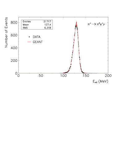
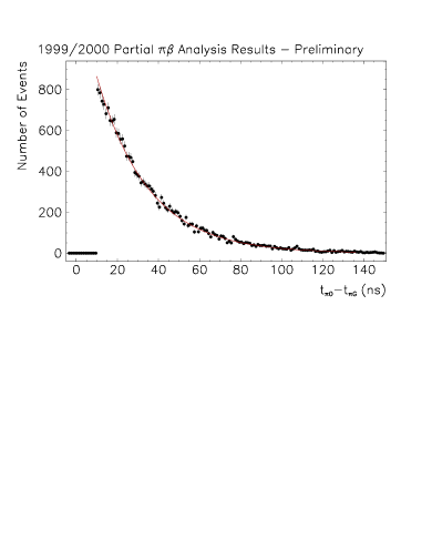
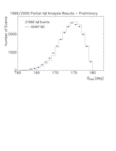
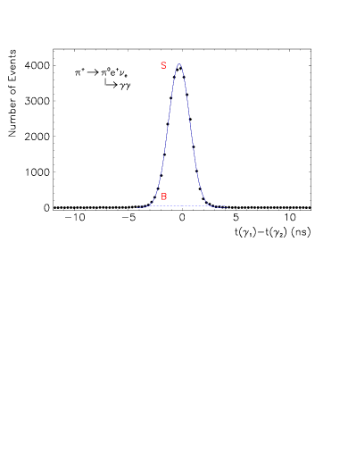
Figure 9: Upper left: $\pi^{0}$ energy spectrum in $\pi\beta$ decay; solid curve: GEANT simulation. Upper right: Histogram of time differences between the beam pion stop and the $\pi\beta$ decay events (dots); curve: pion lifetime exponential curve. A software cut at 10 ns was applied. Lower left: Histogram of the measured $\gamma$-$\gamma$ opening angle in $\pi\beta$ decay events; solid curve: GEANT simulation. Lower right: Histogram of $\gamma$-$\gamma$ time differences for $\pi\beta$ decay events (dots); curve: fit. Signal to background ratio exceeds 250. All plots reflect a subset of the $\pi^{+}\to\pi^{0}e^{+}\nu$ decay data measured in 1999/2000.

The high quality of the PIBETA data is demonstrated in the histograms of the calorimeter energy and event timing (following the $\pi^{+}$ stop time), as well as of the $\gamma$-$\gamma$ opening angle and time difference for a subset of the recorded pion beta decay events, shown in Fig. 9. In particular, the low level of accidental background is evident in the $\gamma$-$\gamma$ relative timing histogram; the peak to background ratio exceeds 250. The histogram of recorded $\gamma$-$\gamma$ opening angles for pion beta events provides possibly the most sensitive test of the Monte Carlo simulation of the apparatus, and of the systematics related to the geometry of the beam pion stopping distribution. The latter is the single largest contributor to the overall uncertainty in the acceptance, and, hence, in the branching ratio.

31 First Results: Pion Beta Decay

The first phase of measurements took place in 1999, 2000 and 2001, resulting in some 60,000 recorded pion beta events. The plots of Fig. 9 are based on a data subset acquired in 1999 and 2000. Our current preliminary working result for the pion beta decay branching ratio, extracted from the above analysis, is

$$BR\simeq 1.044\pm 0.007{\rm(stat.)}\pm 0.009{\rm(syst.)}\times 10^{-8}\ .$$ (117)

Our result is to be compared with the previous most accurate measurement of McFarlane et al. McF85 :

$$BR=1.026\pm 0.039\times 10^{-8}\ ,$$

as well as with the SM Prediction (Particle Data Group, 2002 PDG02proca ):

$BR=$	$1.038-1.041\times 10^{-8}\rm\quad(90\%C.L.)$
	$(1.005-1.008\times 10^{-8}\rm\quad excl.\ rad.\ corr.)$

We see that our working result strongly confirms the validity of the CVC hypothesis and SM radiative corrections Mar86 ; jaus01 ; ciri02 . Another interesting comparison is with the prediction based on the most accurate evaluation of the CKM matrix element $V_{ud}$ using the CVC hypothesis and the results of measurements of superallowed Fermi nuclear decays (Particle Data Group 2002 PDG02proca ):

$$BR=1.037\pm 0.002\times 10^{-8}\ .$$

Thus, our current preliminary working result is in very good agreement with the predictions of the Standard Model and the CVC hypothesis. The quoted systematic uncertainties are being reduced as our analysis progresses. To put this result into broader perspective, we can compare the central value of $V_{ud}$ extracted from our data with that listed in PDG 2002 PDG02proca :

PDG 2002:	$V_{ud}=0.9734(8)$,
PIBETA prelim:	$V_{ud}=0.9771(56)$.

Table 2 summarizes the main sources of uncertainties and gives their values both in the current analysis, and those that are expected to be reached in a full analysis of the entire dataset acquired to date. We have temporarily enlarged the systematic uncertainty quoted in Eq. 117 pending a resolution of the discrepancy found in the RPD channel and discussed in the following section.

Table 2: Summary of the main sources of uncertainty in the extraction of the pion beta decay branching ratio. The column labeled “Partial” corresponds to the present analysis based on a portion of the data taken in the years 1999 and 2000.

	Uncertainties in %
Dataset analyzed:		Partial	Full
external:	pion lifetime	0.019	0.019
	$BR(\pi\to e\nu)$	0.33	$\sim 0.1^{\mathrm{a}}$
	$BR(\pi^{0}\to\gamma\gamma)$	0.032	0.032
internal:	$A(\pi\beta)/A(e\nu)$	0.5	$<0.3$
	$\Delta t(\gamma-e)$	0.03	0.03
	E threshold	$<0.1$	$<0.1$
statistical:		0.7	$\sim 0.4$
total:		$\sim 0.9$	$\lesssim 0.5$
a Requires a new measurement.

32 First Results: Radiative Pion Decay

As was already pointed out, we have recorded a large data set of radiative decays: $\pi^{+}\to e^{+}\nu\gamma$ and $\mu^{+}\to e^{+}\nu\bar{\nu}\gamma$. To date we have analyzed both pion and muon radiative decays, though with more attention devoted to the former, as it is an important physics background to the $\pi\beta$ decay. The radiative pion decay analysis has given us the most surprising result to date, and has commanded significant effort on our part to resolve the issue.

Unlike previous experiments, the different one- and two-arm event triggers used in our experiment are sensitive to three distinct regions in the RPD phase space, resulting in broad coverage. Without going into details, we can loosely label the three phase-space regions according to the positron and gamma energy thresholds ($E^{t}_{e}$, $E^{t}_{\gamma}$) in each region: A (high, high), B (low, high), and C (high, low). Here the low threshold corresponds typically to 20 MeV or less, while the high threshold lies above the Michel decay endpoint, typically 55 MeV or more.

Together, the three regions overconstrain the Standard Model parameters describing the decay, and thus allow us to examine possible new information about the pion’s hadronic structure, or non-(V$-$A) interactions. Appropriate analysis of these data is involved and nuanced, requiring a lengthy presentation; we therefore present here only a brief summary of our results.

Our analysis indicates a measurable departure from SM predictions. Standard Model with the V$-$A electroweak sector requires only two pion form factors, $F_{A}$ and $F_{V}$, to describe the so-called structure-dependent amplitude in RPD. The remainder of the decay amplitude is accounted for by QED in the inner-bremsstrahlung (IB) term. The pion vector form factor is strongly constrained by the CVC hypothesis, while existing data on the radiative pion decay (PDG 2002 PDG02proca ) suggest that $F_{A}\simeq 0.5\,F_{V}$, yielding

$$F_{V}=0.0259\pm 0.0005\ ,\qquad{\rm and}\qquad F_{A}\simeq 0.012\ .$$

Simultaneous as well as separate fits of our data in the three phase space regions confirm the above ratio of $F_{A}/F_{V}\simeq 0.5$. However, they show a statistically significant deficit in RPD yield in one region of phase space, corresponding to high $E_{\gamma}$ and lower $E_{e}$ (mostly in region B), compared to predictions based on the above values of the pion form factors.

A larger deficit in RPD yield, though less statistically significant than our result due to far fewer events, was first reported by the ISTRA collaboration Bol90a ; Bol90b . This first observation was interpreted by Poblaguev Pob90 ; Pob92 as indicative of the presence of a tensor weak interaction in the pion, giving rise to a nonzero tensor pion form factor $F_{T}\sim-6\times 10^{-3}$. Subsequently, Peter Herczeg Her94 found that the existing experimental evidence on beta decays could not rule out a small nonzero value of $F_{T}$ of this order of magnitude. Tensor interaction of this magnitude would be consistent with the existence of leptoquarks Her94 .

Figure 10: Measured spectrum of the kinematic variable $\lambda=(2E_{e+}/m_{\pi+})\sin^{2}(\theta_{e\gamma}/2)$ in $\pi^{+}\to e^{+}\nu\gamma$ decay for the kinematic region B, with limits noted in the figure. Solid curve: fit with the pion form factor $F_{V}$ fixed by the CVC hypothesis, $F_{T}=0$, and $F_{A}$ free. Dashed curve: as above, but with $F_{T}$ also released to vary freely, resulting in $F_{T}=-0.0016\,(3)$. This work is in progress.

We illustrate our working results in Fig. 10 which shows a projected one-dimensional distribution of $\lambda$, a convenient kinematic variable based on $E_{e}$ that ranges from 0 to 1 regardless of $E_{\gamma}$. It is clear that for lower values of $\lambda$ (and therefore of $E_{e}$), an SM fit with only $F_{V},F_{A}\neq 0$ overestimates the experimental yield. Adding a nonzero tensor form factor of $F_{T}\sim-0.0016$ produces statistically significantly better agreement with the data. The fits are two-dimensional and encompass all three kinematic regions. This work is in progress, and the results are subject to change—we are currently refining the analysis as well as the fit strategies.

This working result may be indicating either the existence of a tensor weak interaction, or, alternatively, that the standard treatment of the RPD may not at this time correctly incorporate all known SM physics. Radiative corrections seem to be a particularly good candidate for reexamination.

33 Conclusions

We have extracted an experimental branching ratio for the pion beta decay at the 1 % uncertainty level, and expect to reduce the uncertainty by an additional factor of two in the near future. Our result agrees with the CVC hypothesis and radiative corrections for this process, and it opens the way for the first meaningful extraction of the CKM parameter $V_{ud}$ from a non-baryonic process.

Our analysis of the $\pi\to e\nu\gamma$ decay confirms that $F_{A}/F_{V}\simeq 0.5$, in agreement with the world average. However, events with a hard $\gamma$ and soft e⁺ are not well described by standard theory, requiring “$F_{T}\neq 0$”. We can, though, rule out a large “$F_{T}$”, as reported in analyses of the ISTRA data.

The high statistics and broad coverage of our RPD data in principle guarantee extraction of pion weak form factor values with exceptionally low uncertainties. However, it appears that theoretical treatment of RPD may have to be revisited before the full potential of the PIBETA data is realized.

*Semileptonic Kaon and Hyperon Decays:
What Do They Tell Us about V_us? Semileptonic Kaon and Hyperon Decays:
What Do They Tell Us about $V_{us}$? H.-W. Siebert

34 Introduction

Our best sources of information on $V_{us}$ are semileptonic decays (s.l.d.) of kaons and hyperons. The leptonic part of the matrix element of s.l.d. is unambiguous. In contrast, the hadronic part is modified by $SU_{3}$ symmetry breaking. For kaon s.l.d., which are pure V transitions, this is a minor problem, since for V transitions $SU_{3}$ breaking effects are of second order only (Ademollo-Gatto theorem). On the other hand, s.l.d. of hyperons are mixed vector and axialvector transitions, and there is at present no agreement on the theoretical side how to handle $SU_{3}$ breaking here.

35 Semileptonic kaon decays

Both $K^{+}_{e3}$ and $K_{L,e3}$ decay rates are well-known experimentally since more than 20 years. The experimental situation pdg3 is summarized in table 3. It is seen, that in $K^{+}_{e3}$ decay, the experimental error of the decay rate is dominated by the error of the branching ratio, while in $K_{L,e3}$ decay, the errors of the $K_{L}$ lifetime and the $K_{L,e3}$ branching ratio contribute about equally.

Already in 1984, a value $V_{us}\,=\,0.2196\,(\pm 1.1\%)$ was extracted from the combined $K^{+}$ and $K_{L}$ data leutwyler . Since then, more investigations of the radiative corrections and the $q^{2}$-dependence of the formfactors have not changed the situation: The experimental error is $\approx 0.8$%, the theoretical error is $<1\%$, and we find a safe value $V_{us}\,=\,0.220\pm 0.03$ (see also the discussion in ref. pdg3 and the talk by J. Marciano in these Proceedings).

36 Semileptonic hyperon decays

The experimental information on strangeness-changing hyperon s.l.d. is summarized in table 4. Most of the results are more than 10 years old bour1 ; bour2 ; bour3 ; wise80 ; hsueh88 with the exception of the new results from the KTEV experiment on $\Xi^{0}\to\Sigma^{+}e\overline{\nu}$ decay alavi01 .

The decay rate $\Gamma$ of each decay is proportional to $|V_{us}|^{2}$, but depends also on the formfactor ratio $g_{1}/f_{1}$. Experimentally, the decay rates are calculated from the measured decay branching ratios, using the much better known lifetimes of the mother hyperons. $g_{1}/f_{1}$ has been determined from the Dalitz plot distributions and in some cases from polarization asymmetries. Three cases can be distinguished here: Using a beam of hyperons polarized at production hsueh88 , using $\Lambda$s from $\Xi^{-}$ decays bour2 , which have a longitudinal polarization $P\,=\,\alpha_{\Xi^{-}}\,=\,0.64$ or analyzing the polarization of the daughter hyperon bour1 ; alavi01 .

There are four branching ratio measurements with errors between 2% and 6% and three measurements of the formfactor ratio $g_{1}/f_{1}$ with errors between 0.015 and 0.05. (The experimental errors of the corresponding hyperon lifetimes are always smaller by at least a factor of 2). In good approximation, the decay rates are $\Gamma_{if}\,=\,const.\cdot V_{us}^{2}\cdot(1\,+\,3g_{1}/f_{1})$. From CVC and $SU_{3}$ symmetry, one obtains for the decays $B_{i}\to B_{j}e^{-}\overline{\nu}$ the relation $g_{1}/f_{1}\,=\,f_{ij}\cdot F\,+\,d_{ij}\cdot D$, where $f_{ij}$ and $d_{ij}$ are $SU_{3}$ Clebsh-Gordan coefficients. Therefore, all measured decay rates and $g_{1}/f_{1}$ ratios within the baryon ground state octet can be described by the parameters $V_{us}$, $F$ and $D$. The dependence of $g_{1}/f_{1}$ on $F$ and $D$ is given in the last column of table 4.

Table 3: Experimental data on kaon s.l. decays.

decay	$\tau$ [10-8 s]	BR	$\Gamma$ [10-15MeV]
$K^{+}_{e3}$	1.2384 ($\pm$ 0.2% )	0.0487 ($\pm$ 1.2% )	2.590 ($\pm$ 1.25% )
$K_{L,e3}$	5.17 ($\pm$ 0.8% )	0.388 ($\pm$ 0.7% )	4.938 ($\pm$ 1.05% )

Table 4: Experimental data on strangeness-changing hyperon s.l. decays.

decay	10${}^{4}\cdot$BR	$g_{1}/f_{1}(exp.)$	$g_{1}/f_{1}$ ($SU_{3}$)
$\Lambda\to pe\overline{\nu}$	8.32 $\pm$ 0.14	0.718 $\pm$ 0.015	F + D/3
$\Sigma^{-}\to ne\overline{\nu}$	10.17 $\pm$ 0.34	-0.340 $\pm$ 0.017	F - D
$\Xi^{-}\to\Lambda e\overline{\nu}$	5.63 $\pm$ 0.31	0.25 $\pm$ 0.05	F - D/3
$\Xi^{-}\to\Sigma^{0}e\overline{\nu}$	0.87 $\pm$ 0.17		F + D
$\Xi^{0}\to\Sigma^{+}e\overline{\nu}$	2.62 $\pm$ 0.17	1.3$\pm$0.2	F + D

Are those results consistent?

First we fit four branching ratios and three formfactor ratios from table 4 to the three parameters F+D, D/(F+D) and $V_{us}$, excluding the much less precise results for the $\Xi^{-}\to\Sigma^{0}e\overline{\nu}$ branching ratio and the $\Xi^{0}\to\Sigma^{+}e\overline{\nu}$ formfactor. The result is listed as “fit 1” in table 5. If we include the much more precise value of $g_{1}/f_{1}$ in $n\to pe\overline{\nu}$ decay (fit 2), F+D is pulled towards the neutron decay value and $V_{us}$ moves toward the value found in kaon s.l.d., but the $\chi^{2}$ of the fit becomes worse. Let us look just at the $g_{1}/f_{1}$ values in fig. 11: Here for each decay the $\pm 1\sigma$ contour in the F,D plane from the measured value of $g_{1}/f_{1}$ is shown. There is good consistency between the hyperon decay and the neutron decay values. We also see, that the neutron decay result produces a very strong correlation between F and D, therefore we prefer the parameters F+D and D/(F+D), which are almost uncorrelated in the fit. To demonstrate the precision of the neutron decay result, a dashed line for F+D=1.260 is also drawn. The results are given as “fit 3” in table 5.

Table 5: Fit results.

	F+D	D/(F+D)	$V_{us}$	$\chi^{2}$/NDF
fit 1	1.225$\pm$0.022	0.638$\pm$0.005	0.227$\pm$0.003	11.5/4
fit 2	1.2736$\pm$0.0018	0.639$\pm$0.005	0.223$\pm$0.002	16.1/5
fit 3	1.2737$\pm$0.0013	0.635$\pm$0.006		2.5/2

Figure 11: F and D as determined from $g_{1}/f_{1}$ measurements. The bands from the hyperon s.l. decays correspond to the $\pm\,1\sigma$ contours. The dashed line is for F+D=1.26.

The “fit 3” result then is used to calculate $V_{us}$ for each hyperon s.l.d. from the measured branching ratio. The results are shown in fig. 12. The mean of the four $V_{us}$ values drawn as solid lines is 0.223$\pm$0.004, marked as “hyperons” in fig. 12, with $\chi^{2}$/NDF = 12.7/3. where the error of the mean was increased by a factor $\sqrt{\chi^{2}/NDF}$. This value is in good agreement with the $K_{e3}$ result.

Figure 12: Determination of $V_{us}$ from Kaon and hyperon s.l.d. rates. The dashed result from $\Xi^{-}\to\Sigma^{0}e\overline{\nu}$ decay is not included in the average labelled “hyperons”.

However, this analysis was done without taking $SU_{3}$ symmetry breaking into account. There is at present no agreement between the different attempts to predict the effect of $SU_{3}$ symmetry breaking on $f_{1}$ and $g_{1}$, except that these changes could be up to 10% in some cases. There is not even agreement on whether a given formfactor should become larger or smaller. Table 6, taken from ref. flores98 , lists some calculations by different authors on the change in $f_{1}$, which would directly affect the determination of $V_{us}$ from a given s.l. decay rate (apologies to all authors neglected here). Also, in the calculation of the decay the radiative corrections from ref. Toth have been used. Are they really safe (see ref. glueck , for instance) ?

Table 6: Theoretical estimates of symmetry breaking effects on $f_{1}$. The ratio $f_{1}/f_{1}^{SU(3)}$ is listed.

Transition	ref. flores98	ref. anderson93	ref. donoghue87	ref. krause90	ref. schlumpf95
$\Lambda\to pe\overline{\nu}$	1.02$\pm$0.02	1.024	0.987	0.943	0.976
$\Sigma^{-}\to ne\overline{\nu}$	1.04$\pm$0.02	1.100	0.987	0.987	0.975
$\Xi^{-}\to\Lambda e\overline{\nu}$	1.10$\pm$0.04	1.059	0.987	0.957	0.976
$\Xi^{-}\to\Sigma^{0}e\overline{\nu}$	1.12$\pm$0.05	1.011 0.987	0.943	0.976

To conclude, we find agreement on $V_{us}$ from $K_{e3}$ and from hyperon s.l.d. The special feature of $K_{e3}$ decays being pure vector transitions makes the determination of $V_{us}$ from the $K_{e3}$ data much safer than from the hyperon s.l. decay data. Unless new experimental data differ radically from the existing results, or a much more precise understanding of $SU_{3}$ symmetry breaking and radiative corrections in hyperon s.l.d. emerges, the $K_{e3}$ result will be our best bet on $V_{us}$. So it seems unlikely that $V_{us}$ will change sufficiently to erase the intriguing unitarity deficit…

*Project of a New Measurement of the Electron-Antineutrino-Correlation $a$ Coefficient in Neutron Beta Decay Project of a New Measurement of the Electron-Antineutrino-Correlation $a$ Coefficient in Neutron Beta Decay B.G. Yerozolimsky

Up to date, there were only three attempts to measure this angular correlation coefficient: the first was made in 1967 in Moscow Grigoryev , the second was finished in 1978 in Zeibersdorf Stratova and the last has been done recently at ILL and published in 2002 byrne .

The data derived in these experiments are consistent with each other, but their accuracy does not exceed 5%:

$$\mathbf{a}=-0.091\;\;\pm 0.039\qquad\;\>\cite[cite]{\@@bibref{Authors Phrase1YearPhrase2}{Grigoryev}{\@@citephrase{(}}{\@@citephrase{)}}}$$

$$\mathbf{a}=-0.1017\pm 0.0051\qquad\cite[cite]{\@@bibref{Authors Phrase1YearPhrase2}{Stratova}{\@@citephrase{(}}{\@@citephrase{)}}}$$

$$\mathbf{a}=-0.1054\pm 0.0055\qquad\cite[cite]{\@@bibref{Authors Phrase1YearPhrase2}{byrne}{\@@citephrase{(}}{\@@citephrase{)}}}$$

This situation looks particularly poor if one takes into account that the values of all other parameters which characterize this fundamental beta decay process (lifetime $\mathbf{\tau}$, angular correlation coefficients A and B) are known with much higher precision. This stops possible investigations of validity of the Standard Model Theory of Week Interactions. Thus, measurements of the value of a made with improved accuracy are now urgently needed. Discussions which took place during this Workshop confirm this conclusion.

From our point of view, the main reason of poor accuracy of a–measurements is the methods used in all previous experiments, which required too precise spectrometry of the decay products (electrons and recoil protons). For instance, in the experiment of Prof. J. Byrne, the proton spectrum was measured, and it is too insensitive to the a–value. In order to reach 1% accuracy in a–value the proton spectrum had to be measured with $\sim 3\cdot 10^{-4}$ precision.

The goal of our new approach is to arrange the experimental device in such a manner that events with opposite directions of antineutrino would be reliably separated. Then the value of a can be simply derived by comparing numbers of events in each group, and no precise spectrometry will be needed.

The method of measurement we are going to use is based on two ideas:

First of them was proposed many years ago in our laboratory at Kurchatov Institute in Moscow. It is to arrange two detectors (one for beta-electrons and the second for recoil protons) in 180 degree geometry relative to decay region of the neutron beam. These detectors are switched in coincidences with one another. It can be easily understood that if solid angles of these detectors are sufficiently small and the energy of the detected electrons is not too low ($T_{e}>$ 250 keV) the proton energy spectrum will consist of two groups belonging to decay events with opposite antineutrino directions. These two groups can be easily separated with the help of usual TOF technique without any serious precision.

Unfortunately, in spite of the fact that using this approach one can detect decay events corresponding to definite cones of antineutrino escape angles, the antineutrino–electron angular correlation can not be evaluated from these data because solid angles of antineutrino emission in these two groups are principally different. This method of selecting events with definite antineutrino escape solid angles has been only used in experiments with polarized neutrons (measurements of B correlation coefficient) where the asymmetries measured were connected with the spin-flip, and antineutrino solid angles did not change.

The second idea was proposed by Yu. Mostovoy in 1994 balashov . He has understood how to make these two antineutrino solid angles equal. He proposed to use a distributed set of diaphragms which form a “proton guide” (about 1 m long) leading protons from the neutron decay region to the detector and a strong axial magnetic field inside. In such a case to come to the detector protons must have not a limited flight angle but a limited transverse component of momentum P_p⟂, and as a result, both solid angles of antineutrino become identically equal. This situation is illustrated with the help of a momentum diagram in Fig 13, where a schematic sketch of the measurement arrangement including both ideas is presented too. The value of the transverse momentum limit depends upon the diameter of the diaphragms and the strength of the longitudinal magnetic field. If, for example, a small proton source is disposed on the central axis

$$P_{p\perp}(max)=(eBD)/4c$$ (118)

Where B is the magnetic field in Gs, D – diameter of the diaphragms in cm, e – elementary electric charge and c – velocity of light.

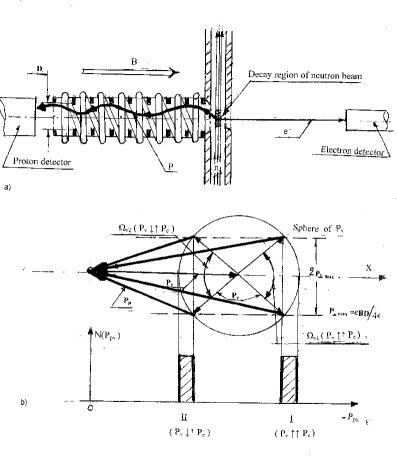
Figure 13: a) The arrangement with the longitudinal magnetic field b) Momentum diagram.

The equality of solid angles of both groups of antineutrino which is evidently seen on the momentum diagram would lead to equality of integrals N₁ and N₂ of the P_px spectrum groups if the angular correlation between the electron and antineutrino momentums would be absent. Thus, in order to measure the a–coefficient one has simply to compare the numbers of events in these groups of the proton TOF spectrum. The measured asymmetry $x=(N_{1}-N_{2})/(N_{1}+N_{2})$ is connected with a–value by a simple formula

$$x=\mathbf{a}\cdot v/c\langle\cos\theta_{e\nu}\rangle$$ (119)

In this equation v/c must be averaged over the spectrum of electrons, and the Cosine of the angle between electron and antineutrino flight directions must be averaged too. To make these calculations one must know the spectrum of electrons detected. Therefore the electron detector must be able to measure these energies. But the requirement for precision of measurements in this case is very moderate: estimations show that uncertainty in the knowledge of electron energy on the level of several keV will cause a methodical error in a essentially lower than the accuracy planned.

All these features look very promising, but there is one problem which can spoil this elegant approach. As it is well seen from the momentum diagram in Fig 13, in order to get the two proton groups of the TOF spectrum well separated one imperative condition must be fulfilled: the maximum transverse proton momentum has to be less than the antineutrino momentums in all decay events recorded. This means that the spectrum of electrons detected must have an upper limit. This requirement which looks from the first sight not very difficult to fulfill appears really to be rather serious due to the presence of low amplitude “tail” in the response curve of all beta-detectors.

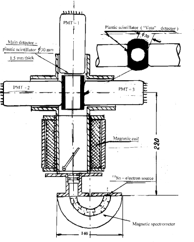
Figure 14: A schematic sketch of the experimental setup at Harvard

The main reason of such property of detectors is backscattering of electrons after hitting the detector - the process which causes the loss of some part of electron energy, which had to be transmitted to the detector. As a result, the two proton groups corresponding to opposite directions of antineutrino are never separated completely, what causes methodical uncertainty in measured values of a. Monte Carlo computer simulations carried out at the Kurchatov Institute in Moscow and at NIST in USA confirmed these conclusions. This was the reason of special investigations carried out at Harvard. Their goal was to investigate this effect and to reduce it as much as possible. In order to exclude the events when electrons are backscattered from the detector we decided to install an additional detector disposed in such a manner that scattered electrons will hit it. Such events can be rejected by an anticoincidence module.

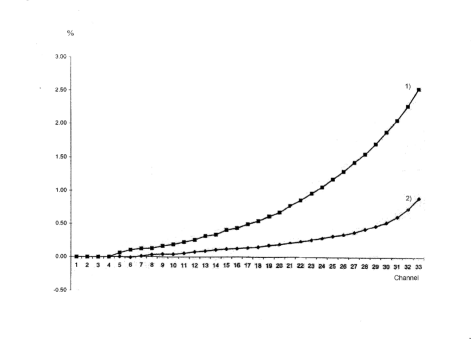
Figure 15: Experimental integral spectrum of low amplitue ”tail” measured with plastic scintillators

This idea was checked during several years with a special experimental set-up in our laboratory at Harvard University. A sketch of one of the last versions of this set-up is shown in Fig 14. A sample of Sn-113 activated in the MIT reactor was used as a conversion electron source. The electron beam emitted by the source was cleaned by a magnetic separator. After cleaning the spectrum of the electrons reaching the detector consisted of a single monochromatic line (360 keV). A solenoid with $\sim$ 250 Gs magnetic field was used to focus the electrons on the detector. The latter was disposed at $\sim$ 30 cm from the exit of the separator. We took measures to prevent electrons to be scattered on the way to the main detector.

An additional detector intended to exclude cases of backscattering (we will call it “veto-detector”) was installed before the main detector. It was a plastic scintillation detector viewed by two photomultipliers. The electrons from the beam came to the main detector through a cylindrical hole made along the axis. The solid angle for catching backscattered electrons was $\sim$ 97% of 2$\pi$. As it was mentioned, the signals from this “veto”–detector activated an anticoincidence circuit, and so, almost all cases when electrons were backscattered had to be excluded.

We investigated several types of main detectors: plastic scintillators, liquid scintillators, Stilben, Si(Li) semiconductor detectors. Best results were obtained with simple plastic detectors. The diameter of scintillator was 30 mm, thickness 1 mm, type of the plastic NE102.

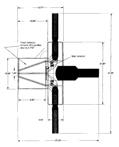
Figure 16: Full-scale model of beta-detector with”Veto”-system build at NIST

The amplitude spectra in Fig 15 demonstrate the effect of the “veto” system.

Curves (1) and (2) present integral spectrums of “tails” ${}_{o}\smallint^{n}y(n)dn$, where $y(n)$ are the numbers of counts in the analyzer channel $n$, in % of “whole spectra” without and with anticoincidences with the “veto”–detector. A 3 – 4 fold reduction of the low-amplitude “tail” in the spectrum is evidently seen.

The residual low–amplitude part of spectra is, most probably, not connected with electron backscattering. Its origin is to be investigated. Preliminary results of our recent experiments show that some part of this effect is connected with the bremsstrahlung of electrons hitting the detector. Calculations carried out at Harvard show that the value of the “tail” now achieved is good enough to go on with the realization of the project.

I will speak now about very important results obtained at NIST. A detailed computer Monte Carlo calculations were carried out there in order to optimize all parameters of the experimental apparatus which is to be built and to estimate all possible sources of methodical errors in a on the level less than 0.5%. Estimations of the “luminosity” of the optimized measuring device showed that the statistical possibilities available on the NIST reactor and moreover at ILL secure the possibility of obtaining the a–value with 1% accuracy during a reasonable period of time. A full-scale model of electron detector with “veto-detector” system based on the same idea as in the experiments at Harvard has been built at NIST too. Fig 16 shows the construction of this model. It was tested on the Van de Graaf accelerator which was a source of monochromatic electrons with the energy about 800 keV. The spectrums obtained confirmed the reduction of the “low-amplitude tail” with the help of “veto” system.

A big team of scientists (listed in the preface to this talk) is busy now with the construction of main parts of experimental set-up needed for realization of this project, and we hope to have grant application ready to the end of this year.

*The Neutron Decay Spectrometer aSPECT
The Neutron Decay Spectrometer aSPECT S. Baeßler, S. Bago, J. Byrne, F. Glück, J. Hartmann, W. Heil,
I. Konorov, G. Petzoldt, Y. Sobolev, M. van der Grinten, O. Zimmer S. BaeßlerS. BagoJ. ByrneF. GlückJ. HartmannW. Heil
I. Konorov G. PetzoldtY. SobolevM. van der GrintenO. Zimmer

37 Introduction

Measurements of the lifetime $\tau_{\rm n}$ and the beta asymmetry $A$ of the free neutron, combined with the muon lifetime, enable us to determine the coupling constants of the weak interaction and the upper left element of the Cabbibo-Kobayashi-Maskawa-Matrix (CKM), $V_{\rm ud}$. The other entries of the upper line of the CKM matrix, $V_{\rm us}$ and $V_{\rm ub}$, are known from high energy physics. Therefore a test of the unitarity of the CKM matrix is possible,

$${\left|V_{\rm ud}\right|}^{2}+{\left|V_{\rm us}\right|}^{2}+{\left|V_{\rm ub}\right|}^{2}=1$$

Traditionally, this test uses $V_{\rm ud}$ as determined by nuclear $0^{+}\to 0^{+}$-decays. Since recently, the above mentioned neutron decay data can be used to calculate an independent value for $V_{\rm ud}$ to a precision that is comparable to that of the traditional method. In both cases, the sum of the squares of the matrix elements of the equation above is too small by $2-3\sigma$ PDG2002baessler ; Hard02 ; Abele02 .

A violation of the unitarity of the CKM matrix would call for the Standard Model to be extended. Although the theoretical corrections to the experimental results could be wrong, the experimental situation also needs to be scrutinised. The most accurate experiments which measured the beta asymmetry $A$ disagree with each other. Several groups are preparing new measurements to improve the accuracy on the beta asymmetry Abele02 ; Dubbers02 ; Young02 .

A different approach is offered by measuring the electron neutrino correlation coefficient $a$ in neutron decay together with the neutron lifetime $\tau_{\rm n}$ to determine $V_{\rm ud}$. The experimental and part of the theoretical systematics are different from those of a beta asymmetry measurement, so that such a measurement of $a$ can give independent information. Unfortunately the present knowledge of $a$ (see Strat78 ; Byrne02 ) is too poor to add meaningful information to the above mentioned problem.

38 Description of the spectrometer aSPECT

The aim of our collaboration is to use the neutron decay spectrometer aSPECT to improve the precision of the knowledge of $a$ by more than an order of magnitude. In the standard model a mesurement of $A$ is equivalent to a measurement of $a$. The desired precision of aSPECT corresponds to an improvement in the beta asymmetry $A$ by a factor of about 5. A measurement of $a$ to that precision can remove the current experimental ambiguity surrounding this problem.

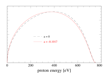
Figure 17: Dependence of the Proton Spectrum on the value of the neutrino-electron-correlation-coefficient $a$. As a comparison a fictious proton spectrum assuming $a=0$ is given. With aSPECT we are able to measure the difference between these spectra with high precision.

The main idea of aSPECT is that the recoil spectrum of the proton in neutron decay is sensitive to the neutrino-electron-correlation coefficient $a$. If the electron and neutrino emerge with parallel momenta, the proton needs to have a high momentum in the opposite direction, whereas otherwise the proton momentum can be small. As a result the value of $a$ shows up as a distortion of the proton recoil spectrum.

So far spectrometers to study nuclear recoils were magnetic spectrometers which could be optimized either for high energy and momentum resolution or for a high acceptance solid angle. aSPECT is a retardation spectrometer which integrates the proton spectrum above an electrostatic barrier. Retardation spectrometers combine a $4\pi$ solid angle with a high energy resolution and are suitable for precision experiments even if the source strength is low.

We define the ratio $r_{h}$ as the count rate of decay protons in the proton detector while a barrier voltage $U$ of about $400\hbox{$\,$}\hbox{\rm V}$ is applied divided by the total count rate (no barrier voltage). If $w(E)$ is the proton spectrum as shown in the picture and $T(E)$ the transmission function of the electrostatic barrier at the barrier voltage $U$, then $r_{h}$ is given by

$$r_{\rm h}=\frac{\int T(E)w(E)dE}{\int w(E)}\quad.$$

If all decay protons would be emitted with momenta parallel to the magnetic field, then $T(E)$ would be a simple step function. The extracted value of $a$ depends on $r_{\rm h}$ in a way which is analytically known.

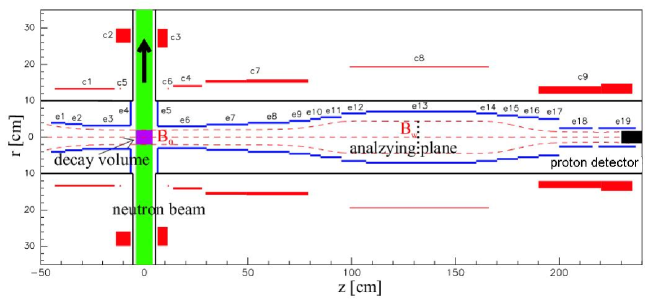
Figure 18: Sketch of the aSPECT spectrometer. The coils are denoted with c1 to c9, the electrodes are e1 to e19. Coils, electrodes (except for e7 and e18) and cryostat are cylindrically symmetric.

A sketch of the setup is shown in figure 18. Unpolarized neutrons are guided through the decay volume of the spectrometer. About one out of $10^{8}$ neutrons decays in the decay volume, the recoil proton is guided by the magnetic field lines. Protons emitted to the left direction are reflected by an electrostatic mirror (electrode e1) so that all protons finally are directed towards the analyzing plane and detector. At the analyzing plane there will be the above mentioned barrier voltage. Protons traveling from the high field $B_{0}\sim 3\hbox{$\,$}\hbox{\rm T}$ to the weak field $B_{\rm w}\sim 0.5\hbox{$\,$}\hbox{\rm T}$ will turn their momenta due to the inverse magnetic mirror effect to be nearly parallel to the magnetic field lines. Therefore our transmission function $T(E)$ is close to the ideal step function. The proton detector which will be a silicon drift detector counts the protons which pass the barrier. Further details can be found in Zimmer00 .

39 Expected systematic uncertainties

Detailed studies were performed to keep the systematic uncertainties at a level which allows for a determination of $a$ with an uncertainty of $\Delta a/a\sim 10^{-3}$.

In our analysis we rely on the transmission function to be precisely known. This requires the following conditions to be met:

• All protons from neutron decay events in the decay volume which are able to pass the analyzing plane can reach it. If so, we can compute the transmission function under the assumption that the proton emission angular distribution in the decay volume is isotropic.

  The protons which are emitted in the wrong hemisphere are reflected back by the mirror electrode e1.

  The magnetic mirror effect is the reflection of protons in an increasing magnetic field. Since the reflection depends on the emission angle of the proton, the magnetic mirror effect introduces a cut in the emission angles. In our setup the magnetic field is decreasing slightly in the decay volume in the direction of the analyzing plane so that the magnetic mirror effect is completely avoided.

  A shallow magnetic field maximum at the analyzing plane helps to ensure that the protons which should pass the analyzing plane are not reflected too early.

• The proton movement can be described in the so-called adiabatic approximation. This is true if the electric and magnetic fields are changing sufficiently slow on a proton trajectory. We checked this assumption for our setup in precise trajectory calculations.

• The electric potential in the analyzing plane is uniform and known accurately, as well as the magnetic fields in analyzing plane and decay volume.

• The detection efficiency of the proton detector does not vary strongly with impact energy, angle, or position.

• Protons which cannot pass the analyzing plane are trapped between it and the electric mirror e1. They have to be removed from the trap before they interact with the rest gas. Our solution is that electrode e7 is a dipole electrode producing en electric field across the magnetic field direction. Due to the $E\times B$ drift the protons are removed from the trap after a few tens of oscillations.

We can thus determine the transmission function by measuring the electric potential in the analyzing plane and the magnetic fields in decay volume and analyzing plane only. The above-mentioned level of systematic uncertainties can be reached if we know the electric potential in the analyzing plane $\Delta U$ better than $10\hbox{$\,$}\hbox{\rm mV}$ and the magnetic fields in decay volume and analyzing plane to a relative accuracy of $\Delta B/B\sim 10^{-4}$. The vacuum has to be as good as $p\sim 10^{-9}\hbox{$\,$}\hbox{\rm mbar}$ to avoid that interactions with the rest gas have a significant impact on the transmission function.

The background count rates can be efficiently determined in auxilliary measurements with an electric potential in the analyzing plane which is higher than the maximum proton energy. The remaining problem is the electron background, caused by electrons emitted in the same decay events as the protons. The electron signal might overlap with the proton signal and this introduces errors in the proton counting. With a second, much stronger $E\times B$ drift electrode (e18) we can move the protons far enough sideways that the positions sensitivity of our detector ensures that electrons and protons coming from the same neutron decay are counted as two separate events. Then electron events can be removed from the count rates in the same way as any other background events.

*Neutron Decay Correlation Measurements
in Pulsed Beams
Neutron Decay Correlation Measurements in Pulsed Beams D. Dubbers

40 The New PERKEO

In a recent publication Abele1 we discussed the CKM matrix element $V_{ud}$ as derived from neutron decay measurements. We came to the conclusion that unitarity of quark mixing is violated in the first row of the CKM matrix at the level of about 3 $\sigma$. The main error in this analysis stems from the neutron beta decay asymmetry $A$. Other quantities which enter the analysis, like the neutron lifetime $\tau$, the strange and bottom matrix elements $V_{us}$ and $V_{ub}$, and the radiative corrections would have to be wrong by about 8 $\sigma$ in order to explain the observed deviation from the Standard Model prediction on unitarity.

As this finding is the result of many years of very careful work, what is needed now is a very significant improvement in the quality of neutron correlation experiments in order to resolve this problem in a satisfactory way. In the following we present an instrument scheme which will strongly improve both the statistical as well as the systematic errors in neutron decay correlation experiments.

Our strategy is the following: Today, in neutron decay, count-rates of up to 300 s^-1 can be achieved Abele1 . However, with the new ”ballistic” supermirror cold-neutron guide H113 which was designed and installed at ILL by our group Haese , the neutron decay rate within the beam (cross-section 20$\times$6 cm²) is incredibly high, namely 2$\times$10⁶ (unpolarized) neutron decays per second and per meter of beam length. However, only a rate of about 10⁴ s^-1 is manageable in the detectors, a rate which would decrease the now dominant statistical error by one order of magnitude. Therefore, if all electrons or protons from neutron decay were collected at H113 over several meters of beam length, then we would have an intensity which is several hundred times higher than needed. As is well known, in this type of experiments one usually can trade the parameter ”count-rate” against improvements in other parameters like background, neutron polarization, or various ”edge” effects. In the following we shall discuss how we can realize such a trade-off with a new instrument now under construction, called ”The New Perkeo”.

The principle of this instrument is rather simple. We apply a magnetic field of B₀ = 1 Tesla along the neutron beam over a length of 3m. The magnetic field serves as guide field for the electrons and protons from neutron decay. They leave the solenoid at both ends, upstream and downstream. There, by additional magnetic fields applied at right angles to B₀, i.e. to the neutron beam direction, the decay products can be spatially separated from the neutron beam and guided to appropriate particle detectors. With a continuous neutron beam passing through this instrument (with a cross section of 6$\times$6 cm²), the count-rate on the detectors will be above 10⁶ s^-1. Of course, this count-rate is far too high to be useful, and systematic errors would be similar as in earlier experiments.

I shall now discuss how to trade most of this count-rate for better systematics. The most obvious trade-off is to sacrifice neutron intensity for higher neutron polarization. Recent investigations at ILL Soldner have shown that with supermirror polarizers one can obtain an average polarization of 99.5% when sacrificing another factor of two in intensity (i.e. 10% instead of the usual 20% transmission).

More such trade-offs can be realized when a pulsed neutron beam is used. Pulsing can be achieved with two beam choppers at 10m distance to each other, with a duty cycle of 65% and 25%, respectively, and a repetition period of 6ms. This set-up produces short neutron pulses of 1.0$\times$10⁸ neutrons in each pulse, and leads to an (unpolarized) peak neutron decay rate of 1.1$\times$10⁵ s^-1. This number includes losses due to further beam-tailoring and corrections for chopper opening time

The detectors are gated ”on” only while the neutron pulse is fully contained within the fiducial volume of the spectrometer. For a 2m long such volume, the duty cycle of the detectors is 13%. The time average neutron decay rate then is 1.4$\times$10⁴ s^-1. Working with the highly polarized neutron beam mentioned above would reduce these numbers by ten.

This beam-chopping scheme will eliminate several further error sources. The other leading error in neutron correlation measurements (besides neutron polarization) is undetected background. In the previous Perkeo instrument, neutrons fly freely, in a high vacuum and without touching any material devices, from the last beam-tailoring orifice, situated 1m upstream of the entrance of the instrument, all the way down to the beam stop, situated 4m downstream of the exit of the instrument. Background (of order 2%) is determined off-line by shutting the beam with a ⁶LiF plate after the last orifice. The error induced by this method is twofold: firstly, this neutron beam shutter itself produces a small background (of order 10^-4 of the incoming beam), of which a tiny amount can reach the detectors and leads to an over- correction of background; secondly, when the neutron beam is on, the beam stop produces a similar amount of uncorrected beam-related background. In previous experiments, these backgrounds could be estimated and required a correction of (0.50 $\pm$ 0.25)% on $A$.

In the new scheme, these background errors are completely eliminated: with a pulsed beam, neutron decay is being measured while the beam is closed by the chopper, that is under exactly the same condition as when background is measured off-line. Secondly, the beam stop can produce no additional background because at the time when the pulsed beam reaches the beam stop the neutron detectors will be gated off.

The next-to-leading error source in our previous experiments is due to magnetic mirror effects in the inhomogeneous B0-field. Electrons or protons spiralling under near 90 in a magnetic field of increasing magnitude will be repelled by the field, and will be counted in the wrong detector. In the new scheme, this effect can be suppressed at will, as in the evaluation of the experiment the length of the active volume, i.e. the region of high uniformity of the B₀-field, can be chosen even after the end of the experiment.

Another unavoidable error source in continuous beam experiments is due to edge effects on the detector. Electrons or protons guided to the detector by the magnetic field may hit the detector near its edge, and be detected or not, depending on their precise trajectory. Also this effect is completely eliminated in the new scheme, as the neutron cloud is, by the magnetic field, projected onto the active area of the detector without coming close to its edge.

So, in ”The New Perkeo”, the four leading error sources of previous experiments will be strongly suppressed or completely eliminated. The remaining experimental errors in $A$ then are the errors due to detector response, on which at present our group is concentrating its efforts. Our aim then is to reduce the error in the CKM-matrix element $V_{ud}$ which is due to the beta decay asymmetry $A$ below the errors of all the other quantities which enter the unitarity check, as mentioned at the beginning of this article.

Due to the high count-rate of the new set-up, only single-rate experiments can be done, but no coincidence measurements. Still, with single-rate experiments one can measure all three allowed correlation coefficients in neutron decay with high precision. In Perkeo, the beta asymmetry $A$ was measured with single electrons and gives information not only on the unitarity of the quark mixing matrix, but also on possible right-handed currents (with main sensitivity to their relative phase), and possibly also on weak magnetism. The single-proton asymmetry from polarized neutron decay gives the antineutrino asymmetry $B$, which is sensitive to the mass of a right-handed W-boson. The electron-neutrino correlation coefficient a is measured from the single-proton intensity spectrum (with unpolarized neutrons), and is as sensitive to the unitarity of quark mixing as is the beta decay asymmetry. In the two latter cases the proton energy spectrum will be measured by time-of-flight, by using an electrostatic chopper.

With the high count-rates available with this instrument also other observables could become measurable which are not accessible with present day’s low count-rate instruments. One could do magnetic spectrometry of the decay electrons to gain additional information on radiative corrections or on the Fierz interference term b, do Mott-scattering of the electrons to measure their helicity spectrum, in order to gain information on the neutrino helicity and on right-handed currents, or even measure the very small helicity of the decay protons.

*TRI$\mu$P – a New Facility for Trapping Radioactive Isotopes

TRI$\mu$P – a New Facility for Trapping Radioactive Isotopes K. Jungmann representing work of the TRI$\mu$P group trimp_group at KVI

The new facility TRI$\mu$P (Trapped Radioactive Isotopes: $\mu$icro-laboratories for fundamental Physics) at the Kernfysisch Versneller Instituut (KVI) in Groningen, The Netherlands, has been designed with the central goal to provide cold radioactive atoms and ions for precise measurements of fundamental symmetries and fundamental interactions in physics Jungmann_02 . There is a common believe that the present Standard Model is embedded in a larger theoretical framework. The TRI$\mu$P facility will allow to contribute to the searches for such a new theory by precision tests of the standard theory Langacker_95 . The concept of TRI$\mu$P Wilschut_99 exploits several major recent developments in different fields of physics, in particular the production of intense radioactive beams and very advanced techniques for cooling and trapping of charged and neutral atomic systems in Penning, Paul or laser traps.

The TRI$\mu$P facility design is based on three main radioactive isotope production mechanisms, i.e. direct, inverse kinematics fusion and evaporation and fragmentation reactions. The best method, beam and target material, will be chosen for each experiment depending on the anticipated production yields. Heavy ion beams from the superconducting AGOR cyclotron, which delivers beams up to the 100 MeV/nucleon region, are directed onto fixed targets. The foreseen reactions favor in general proton rich nuclei.

The created isotopes of interest are separated from the primary beam and other reaction products in a novel designed combined fragment and (gas filled) recoil separator. The ion optical system consists of two pairs of dipole magnets for the primary particle selection and quadrupoles for accurate imaging. It can be tuned for mass and momentum selection. Two possible target positions are provided within the arrangement of magnets: one at its very entrance for fragmentation reactions and another one between the two dipole pairs for inverse kinematics reactions. Gas filling of the separator is essential for good imaging if the reaction products appear in a distribution of electric charge states. With appropriate gas densities concurrent electron capture and stripping processes result in an effective charge for the ions, which determines their trajectory in the ion optical system Leino_97 .

At the exit of the separator the product particles have typically 1 MeV/c momentum. For later trapping it is important that they be slowed down. Moderation to eV energies is foreseen in a high pressure gas cell. Presently detailed measurements of relevant atomic physics processes during slow down in gases are under way at KVI to determine the design parameters of this essential device, where an as high as possible throughput needs to be achieved. Despite high activity in the field of radioactive beam facilities with similar goals there is at present little information available on the behavior of the particles in a very interesting energy range where their velocities are of order $\alpha\cdot c$. This is the order of valence electron velocities of the slower gas and where charge exchange and, in particular, neutralization cross sections are high. Alternate slowing down scenarios which are less generic are also explored.

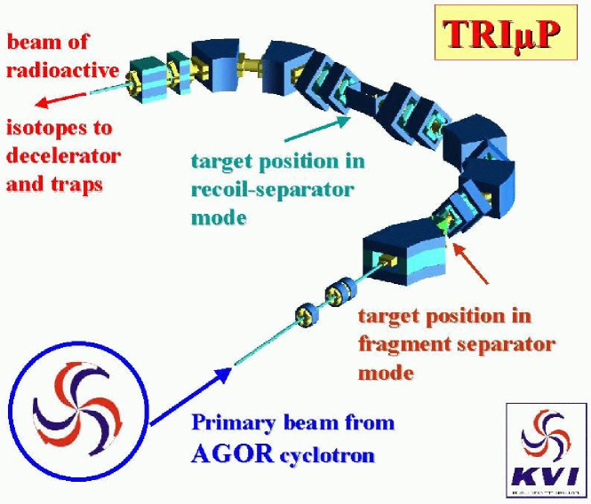
Figure 19: The TRI$\mu$P combined fragment and recoil separator. It is designed to access a large variety of proton-rich isotopes.

Further cooling of the ions, which are expected to be singly charged upon exiting the gas cell slower, occurs in a low density buffer gas. Here the ions are longitudinally guided by an electrostatic potential gradient while at the same time radially confined by a radio frequency quadrupole field. They are collected in a Paul Trap the end voltage of which can be rapidly switched in order to allow this device to act as a beam buncher. After neutralization the atoms can be stored in atoms traps, e.g. a magneto-optical trap.

Research using trapped radioactive atoms and ions is pursued in many laboratories worldwide. It covers a wide range of physics topics in atomic, nuclear and particle physics Schweikhard_00 . The local researchers at KVI concentrate therefore, on two groups of experiments, which are optimal suited for the facility:

• precision measurements of nuclear $\beta$-decays, and

• searches for permanent electric dipole moments in atoms.

In standard theory the structure of weak interactions is of the V-A type, where V and A are vector and axial-vector currents with opposite relative sign causing a left handed structure of the interaction and parity violation Herczeg_01 . Other possibilities which could explain four fermion interactions like $\beta$-decays which are of scalar, pseudo-scalar and tensor type would be clear signatures of new physics. In particular, right-handed currents would also give rise to deviations from standard theory predictions. An observation of a particle behavior in $\beta$-decay which is not V-A type can be expected to shine some light onto the mysteries behind parity violation.

The double differential decay probability $d^{2}W/d\Omega_{e}d\Omega_{\nu}$for a $\beta$-radioactive nucleus is related to the electron and neutrino momenta $\vec{p}$ and $\vec{q}$ through

$$\frac{d^{2}W}{d\Omega_{e}d\Omega_{\nu}}\sim 1+a~{}\frac{\vec{p}\cdot\vec{q}}{E}+b~{}~{}\sqrt{1-(Z\alpha)^{2}}~{}~{}\frac{m_{e}}{E}$$

$$+<\vec{J}>\cdot\left[A~{}~{}\frac{\vec{p}}{E}+B~{}~{}\vec{q}+D~{}~{}\frac{\vec{p}\times~{}\vec{q}}{E}\right]$$ (120)

$$+<\vec{\sigma}>\cdot\left[G~{}~{}\frac{\vec{p}}{E}+Q~{}~{}\vec{J}+R~{}~{}<\vec{J}>\times~{}\frac{\vec{q}}{E}\right]$$

where $m_{e}$ is the $\beta$-particle mass, $E$ its energy, $\vec{\sigma}$ its spin, and $\vec{J}$ is the spin of the decaying nucleus. Among the coefficients in equation (Status of the Cabibbo-Kobayashi-Maskawa Quark-Mixing Matrix) D describes the correlation between the neutrino and $\beta$-particle momentum vectors for spin polarized nuclei and is time reversal violating in nature. It renders a particularly high potential for further restricting parameters in speculative models. The coefficient R relates is highly sensitive within a smaller set of models, since in this region there exist some already well established constraints, e.g., from searches for a permanent electric dipole moment (edm) of fundamental particles. In such experiments, the neutrino momentum cannot be determined directly in a meaningful way. Therefore the recoiling nucleus will be detected instead. The neutrino momentum can then be reconstructed from the kinematics of the process. Since the recoil nuclei have energies typically a few 10 eV, precise measurements can only be performed, if the decaying isotopes are suspended using sufficiently shallow potential wells. Such exist in magneto-optical traps, where neutral atoms are stored at temperatures below 1 mK. Since the atoms must have suitable spectral lines for optical trapping, since also the nuclear properties must be such that rather clean transitions can be observed, and since a precision determination of parameters requires high statistics, i.e. high decay rates, the isotopes of primary interest for the KVI experimenters are ^20,21Na and ^18,19Ne.

An edm of any fundamental particle violates both parity and time reversal symmetries Khrip_97 . With the assumption of a generally valid CPT invariance a permanent dipole moment also violates CP. CP violation, such as it is known from the K and B systems, induces edm’s for all particles through higher order loops. Their values are for any known system at least 4 orders of magnitude below the present experimentally established limits. It should be noted that the known sources of CP violation are not sufficient in Sakharov’s model for the baryon asymmetry, i.e. the dominance of matter over anti-matter in the universe Trodden_99 . New sources of CP violation need to be discovered. Indeed, a large number of speculative models foresees edm’s which could be as large as the present experimental bounds. Historically the non-observation of any edm has ruled out more speculative models than any other experimental approach in all of particle physics Ramsey_99 .

Permanent electric dipole moments have been searched for in various systems with different sensitivities Commins_94 ; Bailey_78 ; Aciari_98 ; Cho_89 ; Harris_99 ; Romalis_01 . Since the searched for, yet unknown, new fundamental forces may act completely different on various particles and systems, a comparison of experiments solely on the basis of the smallest limit in units of $e\cdot cm$ is not possible. Careful and detailed analysis is indispensable. In composed systems such as molecules or atoms fundamental particle dipole moments can be enhanced significantly Sandars_01 . Particularly in polarizable systems where large internal fields can exist. Ra atoms in excited states are of particular interest for edm searches, because of the rather close lying $7s7p^{3}P_{1}$ and $7s6d^{3}_{2}$ states the a significant enhancement has been predicted Dzuba_01 . This gives a several orders of magnitude advantage over the ¹⁹⁹Hg atom, the system which has given the best limits so far Romalis_01 . Further enhancements have been predicted in Ra isotopes with strongly octupole deformed nuclei. Speculative models would allow to observe an atomic edm in Ra already at an absolute value some three orders of magnitude below the present limit set by Hg!

Table 7: Limits on Permanent Electric Dipole Moments $d$ for electrons ($e$) Commins_94 , muons ($\mu$) Bailey_78 , tauons ($\tau$) Aciari_98 , protons ($p$) Cho_89 , neutrons ($n$) Harris_99 , and the mercury atom (${}^{1}99$Hg) Romalis_01 . The new Physics Limits correspond to the predicted highest values among various models beyond standard theory.

	Present Limit	on	Standard Model	New Physics
	$|d|$		Prediction	Limits
	[10-27	e cm]	[10-27e cm]	[10-27e cm]
$e$	$<1.6$	(90% C.L.)	$\stackrel{{\scriptstyle<}}{{\sim}}10^{-11}$	$\stackrel{{\scriptstyle<}}{{\sim}}1$
$\mu$	$<1.05\cdot 10^{9}$	(95% C.L.)	$\stackrel{{\scriptstyle<}}{{\sim}}10^{-8}$	$\stackrel{{\scriptstyle<}}{{\sim}}200$
$\tau$	$<3.1\cdot 10^{11}$	(95% C.L.)	$\stackrel{{\scriptstyle<}}{{\sim}}10^{-7}$	$\stackrel{{\scriptstyle<}}{{\sim}}1700$
$p$	$-3.7\,(6.3)\cdot 10^{4}$		$\sim 10^{-4}$	$\stackrel{{\scriptstyle<}}{{\sim}}60$
$n$	$<63$	(90% C.L.)	$\sim 10^{-4}$	$\stackrel{{\scriptstyle<}}{{\sim}}60$
199Hg	$<0.21$	(90% C.L.)	$\sim 10^{-6}$	$\stackrel{{\scriptstyle<}}{{\sim}}0.2$

From a technological point of view Ra atoms well accessible spectroscopically and a variety of isotopes can be produced in fusion and evaporation or in fission reactions. The advantage of an accelerator based Ra experiment is apparent, because a nuclear edm requires an isotope with spin. and all Ra isotopes with finite nuclear spin are relatively short-lived.

TRI$\mu$P at KVI is expected to offer new possibilities to study with high precision fundamental interactions in physics and fundamental symmetries in nature. The approach combines nuclear physics, atomic physics and particle physics in experimental techniques as well as in the conceptual approaches. The scientific approach chosen in TRI$\mu$P can be regarded as complementary to such high energy physics.

For TRI$\mu$P there exists also a large variety of possibilities for research with cold radioactive isotopes in connection with applied sciences. For example, cold polarized $\beta$-emitters could be the basis for extending the method of $\beta$-NMR, which is very successful in bulk material Fick_00 , to condensed matter surfaces, on which such atoms could be softly deposited.

At KVI a user facility is created which is open to the worldwide scientific community. TRI$\mu$P is jointly funded by FOM (Stichting voor Fundamenteel Onderzoek der Materie, Dutch funding agency) and the Rijksuniversiteit Groningen in the framework of a managed programme. TRI$\mu$P is expected to receive a 50% share of the AGOR beam time. The time planning foresees that the facility is set up by 2004 followed by an exploitation phase until 2013. First physics experiments are expected in 2004. The facility is open for outside users worldwide and proposals are highly welcome.

*Progress Towards Measurement of the Neutron Lifetime Using Magnetically Trapped Ultracold Neutrons

Progress Towards Measurement of the Neutron Lifetime Using Magnetically Trapped Ultracold Neutrons

P. R. HuffmanK. J. CoakleyS. N. DzhosyukR. GolubE. KorobkinaS. K. LamoreauxC. E. H. MattoniD. N. McKinseyA. K. Thompson
G. L. YangL. YangJ. M. Doyle

41 Introduction

We present a progress report on a measurement of the neutron lifetime using three-dimen-sional magnetic confinement of neutrons Doy94 . For detailed information on the experiment, the reader is directed to the graduate theses of Carlo Mattoni Mat02 and Daniel McKinsey McK02 and references Doy94 and Huf00 . This paper summarizes the improvements made to the experiment since the demonstration of three-dimensional magnetic confinement in 1999 Huf00 and shows some preliminary diagnostic data taken with the new setup.

In the 1999 proof-of-principle experiment, approximately 500 UCN were trapped per loading cycle and their decay was observed with a 31 % detection efficiency. The neutron lifetime estimated from two months running time was $660^{+290}_{-170}$ s Bro00 , which is consistent with the accepted value of the neutron beta-decay lifetime of 886 s. The error in estimating the neutron lifetime was primarily due to the fact that the signal to background ratio was approximately 1 to 20.

Various improvements in the apparatus and experimental techniques were made in order to increase the signal to background ratio, increase the signal, and improve the statistical sensitivity to the neutron lifetime. A large number of changes were made to the apparatus and a careful assessment of the neutron activation and neutron-induced luminescence properties of all materials exposed to the neutron beam was performed. In our work thus far, the entire cold neutron beam, only a small fraction of which is in the wavelength region that contributes to single phonon UCN production, was introduced into the apparatus. In an effort to increase signal to background ratio, a 0.89 nm monochromator was developed. Changes made to the cryostat and its contents include a larger magnetic trap and trapping region and a new superfluid helium-filled heat link connecting the cell to the dilution refrigerator. The detection system was also substantially overhauled. Changes include larger light collection optics and detectors, utilizing an optically clear neutron beamstop, and the switch from embedding the wavelength shifter in a clear plastic matrix optically coupled to a plastic tube to evaporating the wavelength shifter onto a diffuse reflector. A new data acquisition system was installed. The results from running the trapping experiment for about one week are presented.

42 Materials Activation and Luminescence

We have studied the low temperature ($\sim 4.2$ K) activation and luminescence properties of a variety of materials present in our trapping apparatus Mat02 . None of the weak neutron absorbers studied (acrylic, graphite, wavelength shifter, or diffuse reflector) displayed any detectable neutron-induced luminescence.

Strong luminescence, of the order of $10^{5}$ s^-1 initially after capture of $\sim 10^{11}$ cold neutrons, was observed for the neutron absorbers boron nitride and lithium fluoride. By comparing the rates of luminescence on two photomultiplier tubes to the rate of their coincidence, a limit on fraction of luminescence events producing more than one correlated photon was set as $<10^{-3}$. Although BN is an appealing shielding material due to its availability in high purity form and its easy machinability, its strong luminescence is a concern. An alternative shielding material, boron carbide, did not display any measurable luminescence. Since B₄C is extremely difficult to machine, we continued to use BN as a neutron absorber but shielded the detectors from BN’s luminescence light using a thin ($\sim 0.5$ mm) layer of graphite as a light absorber.

Of the optically transparent neutron absorbers tested – LiF, B₂O₃, and a boron/lithium glass – strong luminescence was observed only in LiF. The B₂O₃ displayed a time varying signal consistent either with luminescence with $\sim 10^{-3}$ intensity relative to that of LiF or with activation. The boron/lithium glass did not display any measurable luminescence. All three of these materials are subject to some activation concerns. The fluorine in LiF becomes activated by the ¹⁹F(n,$\gamma$)²⁰F reaction. Since ²⁰F decays with a lifetime of 16 s, which is much shorter than the neutron beta-decay lifetime of 886 s, it may be sufficient to simply wait for any activated fluorine to decay. The production of ¹⁸F from the ¹⁶O(T,n)¹⁸F reaction (the tritons are produced in neutron capture on lithium) in the boron/lithium glass and ¹³N from the ¹⁰B($\alpha$,n)¹³N reaction (the alphas are produced in neutron capture on boron) in B₂O₃ may be much more problematic due to their longer lifetimes. Due to the strong ¹⁸F decay signal observed in the boron/lithium glass, and the intense luminescence observed in LiF, B₂O₃ was chosen as the beamstop material for the neutron trapping measurements. Initial estimates indicated that the signal from the B₂O₃ was consistent with the activation of ¹³N. Separate high-flux measurements of this reaction indicate that ¹³N production is roughly three orders of magnitude weaker.

43 Monochromator

The production of UCN by single phonon downscattering of cold neutrons from superfluid helium (the “superthermal process” Gol91 ) requires input neutrons only in a narrow wavelength band around 0.89 nm. Only a small fraction ($<1$ %) of the spectrum of the cold neutron beam at the NG-6 guide at the NIST Center for Neutron Research, where the experiment is located, lies within the relevant wavelength band for production. Thus, for the neutron lifetime measurement, all other cold neutrons contribute mainly to backgrounds. The signal to background ratio of the experiment can be substantially improved by filtering the cold neutron spectrum such that the only neutrons entering the trapping apparatus are those that can produce UCN by single phonon downscattering.

An 0.89 nm monochromator has been constructed using stage 2 potassium-intercalated graphite. The monochromator, tiled from nine pieces, has a total size of 6 cm by 15 cm. The individual monochromator pieces have high stage purity and mosaics varying from 1^∘ to 2^∘. The monochromator reflects more than 80 % of the incident 0.89 nm neutrons, while reflecting less than 2 % of the total cold neutron beam. The incident and reflected beams are shown in Fig. 20. The signal to neutron-induced-background in the magnetic trapping experiment is thus improved by a factor of 40 through use of the monochromator. A detailed description of the monochromator can be found in Ref. Mat02 .

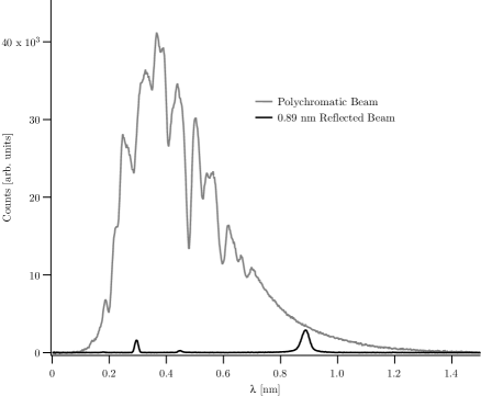
Figure 20: The time-of-flight spectrum of the incident and reflected neutron beams. The reflected monochromatic beam has the $\lambda/2$ and $\lambda/3$ peaks filtered from the beam using pyrolytic graphite and polycrystalline bismuth.

44 Apparatus

The cryogenic apparatus used for the proof-of-principle magnetic trapping measurements is described in detail in Bro00 . The changes made to the apparatus since 1999 will be outlined below and are described in detail in Mat02 and McK02 . The existing cryostat was modified to make room for a larger bore magnetic trap and the accompanying light detection system. The new magnet was designed to be the largest Ioffe-type magnet assembly that would fit in the existing cryostat. Inside of the bore of this new magnet was inserted a larger neutron trapping and detection cell. The cell is coupled to the dilution refrigerator using a superfluid heatlink that provides considerably higher thermal conductance and lower eddy current heating than the copper heatlink used previously.

44.1 Heat Link

The fill lines and heat link between the mixing chamber of the dilution refrigerator and the horizontal trapping region were replaced. In the previous design, the heat link between the mixing chamber and the cell was provided by copper rods and braids, while the cell was filled with ultrapure helium through two 3.2 mm stainless steel lines. This design was susceptible to eddy-current heating of the large copper mass when the magnet current was changed. Furthermore, the heat link had poor thermal conductivity, limited by the braid. Since the new apparatus was designed for higher magnetic fields and with a smaller separation between the magnet coils and the heat link, estimates of the large size of the eddy current heating necessitated a new design.

A continuous cylindrical volume of helium (approximately 5 cm² in area) now extends from the mixing chamber to the horizontal cell. The use of superfluid helium rather than copper results in a much greater thermal conductance for this heat link compared with the previous one. The previous heat link had a measured conductance of $2.3\times 10^{-4}$ W K^-1 at 200 mK Bro00 . A thermal conductance of $0.81~{}T^{3}$ W K^-1, where $T$ is the temperature of the mixing chamber in Kelvin was measured for the new design McK02 .

A small buffer volume provides the thermal link between the superfluid helium heat link and the mixing chamber of the dilution refrigerator. This volume contains copper fins coated with silver sinter to maintain high thermal conductivity between the mixing chamber and superfluid, even at temperatures $<100$ mK, where the Kapitza boundary resistance due to phonon mismatch is significant.

44.2 Magnet

The magnetic trap used in this work is in the Ioffe configuration. Four racetrack-shaped coils are arranged to produce the radially-confining magnetic quadrupole. Axial confinement is provided by two solenoid assemblies with identical current senses.

The magnetic trap used to demonstrate magnetic trapping of UCN in 1999 had an inner bore of 50 mm, and ran at a maximum current of 180 A, corresponding to a trap depth of 1.0 T. The newly constructed magnetic trap was designed to have a considerably larger volume and maximize the number of trapped neutrons. The design was constrained by the size of the helium bath inside the current dewar. The new design was constructed using coils of $2.5~{}\mbox{cm}\times 2.5$ cm cross-section, with a bore diameter of 105 mm. With a larger bore size, a higher detection efficiency could be obtained, as light could be more easily extracted from the trapping region. Also, the larger trap volume allowed the confinement of approximately ten times more neutrons than in with the previous trap.

The trap depth is defined as the difference between the maximum and minimum values of the magnetic field within the confinement region. In our case the maximum magnetic field value is found at the radial edge of the trap, which is defined by the location of the cell walls at a radius of 4.2 cm. The trap depth is 1.1 T for an operating current of 170 A.

44.3 The Detection Insert

The detection insert is based on tetraphenyl butadiene (TPB) evaporated on a 1 mm thick GoreTex sheet, rolled up into a tube and inner diameter of 8.4 cm. The density of the evaporated layer is between 200 $\mu$g cm^-2 and 400 $\mu$g cm^-2. Extreme ultraviolet (EUV) scintillation light is produced by the recoil of neutron decay electrons through the superfluid helium filling the trapping region. TPB absorbs photons over a broad wavelength region from the soft UV to X-rays and emits blue light with a spectrum peaked at 440 nm and a width of approximately 50 nm Bur73 . The fluorescence efficiency of an evaporated TPB film is approximately 1.4.

The great majority ($>$ 80 %) of the scintillation light from the prompt singlet decay of the excited helium is emitted within 20 ns of the ionization event. Each neutron decay event creates a bright flash of EUV light, which is converted to a pulse of blue light by the wavelength shifter. This visible light is transported to room temperature through windows and light guides, and is detected by photomultiplier tubes (PMTs) at room temperature. In this way, neutron decay events result in bursts of photoelectrons, which are detected and recorded.

In order for the TPB fluorescence to be collected by light guides and transported to room temperature, it must pass through an optically transparent, neutron-absorbing disc of boron oxide located at the end of the trapping region. The difficulty with boron oxide is that it clouds up when exposed to atmosphere (it is hygroscopic). However, we found that by minimizing its exposure to the atmosphere, its transparency could be maintained within acceptable limits. It was polished, then stored under vacuum. We found that it could be kept in the atmosphere for up to 15 min. before clouding significantly.

Following the beam dump is a ultraviolet transmitting grade acrylic light guide of diameter 8.7 cm and length 40.7 cm that transports light from the Gore-Tex tube to the end of the experimental cell. The light guide is wrapped in a 175 $\mu$m thick layer of Tyvek to increase its light transport efficiency. Scintillation light that passes out of the light guide then passes through acrylic and quartz windows at 4 K and into a 35 cm long, 11.4 cm diameter light guide that transports the scintillation light from 77 K to 300 K. At room temperature, the scintillation light is split into two photomultipliers and detected in coincidence.

The detector was calibrated by placing a ¹¹³Sn beta source in the center of the insert. Using a single photomultiplier at the end of the 77 K light guide, it was found that the 364 keV beta from the ¹¹³Sn source caused an average signal of approximately 30 photoelectrons.

The efficiency of the light guide splitter was determined by comparing the peak channel position with one photomultiplier to the peak channel position with the splitter installed and two photomultipliers attached. It was found that the light guide splitter is 94 % efficient.

45 Data Acquisition System

The goal of the new DAQ is to record multi-photon scintillation events originating within the cell, and reject events produced by cosmic ray muons. Hence, the data acquisition system triggers when coincident pulses are observed on the two main detection photomultipliers which are not coincident with an event on any of the muon paddles surrounding the trapping apparatus. For each trigger, the data acquisition records the time of occurrence and the digitized waveforms from the two main PMTs. The waveforms are recorded using two 500 MHz PCI digitizer cards. The timing signals and diagnostic information are recorded in a separate timer/counter card. Each event trace is recorded to disk for offline analysis.

46 Progress to Date

The neutron trapping apparatus was operated on several occasions in the spring of 2001 and the fall of 2002. This section contains data during the 2002 runs. It compromises approximately one week of actual trapping data. Note that although the data looks promising, considerably more data must be taken to fully investigate systematic effects. This data collection is now in progress.

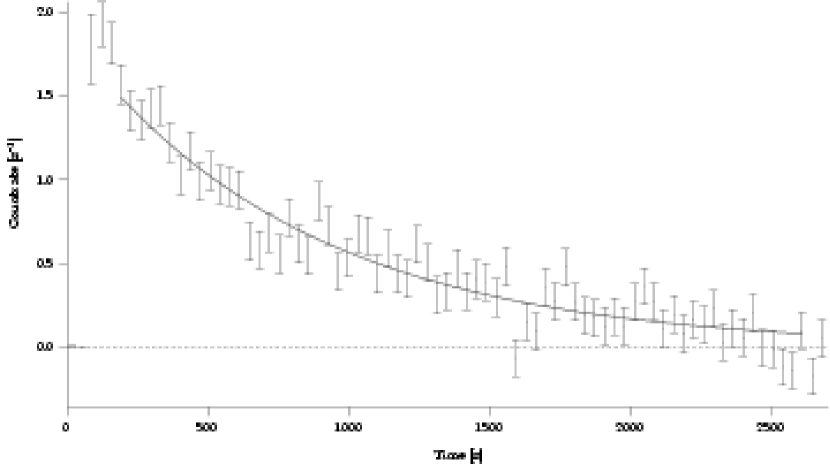
Figure 21: The difference of the positive and negative data collection runs for approximately one week of data. The curve is a fit to the function $y=Aexp(-t/\tau)$ with fit parameters $A=(1.88\pm 0.07)$ s^-1 and $\tau=(834^{+39}_{-36})$ s and a $\chi^{2}=1.2$. If the data is fit to $y=y_{0}+Aexp(-t/\tau)$, where the presumably zero constant offset is allowed to vary, one obtains values of $A=(1.87\pm 0.07)$ s^-1, $\tau=(848^{+104}_{-84})$ s, and $y_{0}=(-0.008\pm 0.052)$ s^-1. Note that the one standard deviation errors quoted are purely statistical and the data is very preliminary.

The presence of time-dependent backgrounds necessitates taking what we refer to as “positive” and “negative” runs. In positive runs, the magnet is energized while neutrons are loaded into the trap. After the beam has been turned off, the neutron decay events are recorded. In negative (or background) runs, the magnet is deenergized while the beam is on, then raised to the full value as the neutron beam is turned off. In this negative case, the backgrounds from neutron activation, etc. should be similar. A difference in the countrate versus time between positive (trapped UCN + backgrounds) and negative (backgrounds only) runs should be magnetically trapped UCN. If for some reason the backgrounds are not identical in the positive and negative runs, then the subtraction process will leave a residual difference which could mimic a trapping signal. Measurements made with natural abundance helium can then be used to determine if a putative trapping signal is caused by imperfect background subtraction.

Analysis of the data is performed by integrating the pulse area of the PMT signals and applying appropriate lower level cuts on the area of the pulses. Since luminescence is known to be present in the coincidence data with thresholds at single photoelectron levels, thresholds are typically set to require an area in each pulse to be equivalent to at least three photoelectrons. Data from all positive runs and all negative runs are pooled and subtracted to yield a difference curve as shown in Fig. 21.

The absolute detection efficiency has not been determined for the detector configuration used above, so the total number of neutrons contained in the trap is not known. We estimate, however, that the number is consistent within a factor of two of the expected number trapped.

47 Future Directions

Our present plan is to take a similar set of data using a natural isotopic abundance helium sample in order to study backgrounds. With this sample, the lifetime of UCN within the trap is less than 1 s due to absorption of the UCN by ³He. Similar positive and negative data will be taken to verify that the decaying signal seen above arises from trapped neutrons.

Once complete, we hope to take a considerably longer set of trapping data to lower the errors on the lifetime to roughly $\pm 10$ s. This should allow us to more carefully study systematic effects. Studies of the temperature dependence of the storage time due to phonon upscattering is also planned.

Ultimately, any technique for measuring the neutron lifetime will be limited by systematic as well as statistical errors. The limiting systematic errors of bottle and beam lifetime measurements, wall interactions and flux measurement, respectively, are not relevant when measuring the neutron lifetime using magnetically trapped neutrons. The use of a magnetic trap prevents interactions with material walls, and the continuous measurement of the neutron decay rate makes an independent measurement of the neutron flux unnecessary. The limiting systematic errors for the magnetic trapping technique are expected to be non-beta-decay loss mechanisms for trapped UCN. All known loss mechanisms, including capture on ³He, single- and multi-phonon upscattering, neutron depolarization (Majorana flips), and marginal trapping, are expected to result in loss rates less than $10^{-5}$ times the beta-decay rate Doy94 ; Bro00 . Another proposed systematic error, the modification of the free neutron lifetime due to nuclear interactions with the surrounding helium, is calculated to have even less of an effect Bro00 . In principle, the measurement of the neutron lifetime using magnetically trapped UCN should remain statistics limited until the fractional error reaches $10^{-5}$. The imperfect subtraction of time-dependent backgrounds can also introduce a systematic error into the measurement. This type of effect will be studied in the coming months.

48 Acknowledgments

Neutron facilities used in this work were provided by the NIST Center for Neutron Research. This work was supported in part by the National Science Foundation under grant No. PHY-0099400.

*Measurement of the Neutron Lifetime
by Counting Trapped Protons Measurement of the Neutron Lifetime
by Counting Trapped Protons F. E. Wietfeldt, M. S. Dewey, D. M. Gilliam, J. S. Nico, X. Fei, W. M. Snow, G. L. Greene, J. Pauwels, Eykens, A. Lamberty,
J. Van Gestel F. E. Wietfeldt, M. S. Dewey, D. M. Gilliam, J. S. Nico, X. Fei, W. M. Snow, G. L. Greene, J. Pauwels, Eykens, A. Lamberty,
and J. Van Gestel

We measured the neutron lifetime at the cold neutron beam NG6 at the National Institute of Standards and Technology (NIST) Center for Neutron Research, using the quasi-Penning trap method first proposed by Byrne, et al.. This method is described in detail in previous publications PTmeth . Figure 22 shows a sketch of the experimental configuration. A proton trap of length $L$ intercepts the entire width of the neutron beam. Neutron decay is observed by trapping and counting decay protons within the trap with an efficiency $\epsilon_{p}$. The neutron beam is characterized by a velocity dependent fluence rate $I(v)$. The rate $\dot{N_{p}}$ at which decay protons are detected is proportional to the mean number of neutrons inside the trap volume:

$$\dot{N_{p}}=\frac{\epsilon_{p}L}{\tau_{n}}\int_{A}da\,I(v)\frac{1}{v}.$$ (121)

where $A$ is the beam cross sectional area, After leaving the trap, the neutron beam passes through a thin foil of ⁶LiF. The probability for absorbing a neutron in the foil through the ${}^{6}{\rm Li}(n,t)^{4}$He reaction is inversely proportional to the neutron velocity $v$. The reaction products, alphas or tritons, are counted by a set of four silicon surface barrier detectors in a well-characterized geometry. We define the efficiency for the neutron detector, $\epsilon_{o}$, as the ratio of the reaction product rate to the neutron rate incident on the deposit for neutrons with thermal velocity $v_{o}=2200$ m/s. The corresponding efficiency for neutrons of other velocities is $\epsilon_{o}v_{o}/v$. Therefore, the net reaction product count rate $\dot{N_{\alpha}}$ is

$$\dot{N_{\alpha}}=\epsilon_{o}v_{o}\int_{A}da\,I(v)\frac{1}{v}.$$ (122)

The integrals in Eq. (121) and Eq. (122) are identical; the velocity dependence of the neutron detector efficiency compensates for the fact that the faster neutrons in the beam spend less time in the decay volume. This cancellation is exact except for a correction due to the finite thickness of the ⁶LiF foil (+5.4 s), and we obtain the neutron lifetime $\tau_{n}$ from the experimental quantities $\dot{N_{\alpha}}/\dot{N_{p}}$, $\epsilon_{o}$, $\epsilon_{p}$, and $L$.

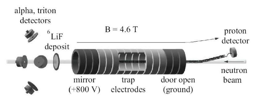
Figure 22: Schematic representation of the experimental method (not to scale).

The proton trap was a quasi-Penning trap, composed of sixteen annular electrodes, each 18.6 mm long with an inner diameter of 26.0 mm, cut from fused quartz and coated with a thin layer of gold. Adjacent segments were separated by 3 mm-thick insulating spacers of uncoated fused quartz. The dimensions of each electrode and spacer were measured to a precision of $\pm 5$ $\mu$m using a coordinate measuring machine at NIST. Changes in the dimension due to thermal contraction are below the 10^-4 level for fused quartz. The trap resided in a 4.6 T magnetic field and the vacuum in the trap was maintained below $10^{-9}$ mbar.

In trapping mode, the three upstream electrodes (the “door”) were held at +800 V, and a variable number of adjacent electrodes (the “trap”) were held at ground potential. The subsequent three adjacent electrodes (the “mirror”) were held at +800 V. We varied the trap length from 3 to 10 grounded electrodes. When a neutron decayed inside the trap, the decay proton was trapped radially by the magnetic field and axially by the electrostatic potential in the door and mirror. After some trapping period, typically 10 ms, the trapped protons were counted. The door was “opened”, i.e. the door electrodes were lowered to ground potential, and a small ramped potential was applied to the trap electrodes to assist the slower protons out the door. The protons were then guided by a 9.5^∘ bend in the magnetic field to the proton detector held at a high negative potential (-27.5 kV to -32.5 kV). After the door was open for 76 $\mu$s, a time sufficient to allow all protons to exit the trap, the mirror was lowered to ground potential. This prevented negatively charged particles, which may contribute to instability, from accumulating in any portion of the trap. That state was maintained for 33 $\mu$s, after which the door and mirror electrodes were raised again to +800 V and another trapping cycle began. Since the detector needed to be enabled only during extraction, the counting background was reduced by the ratio of the trapping time to the extraction time (typically a factor of 125). Figure 23 shows a plot of proton detection time for a typical run.

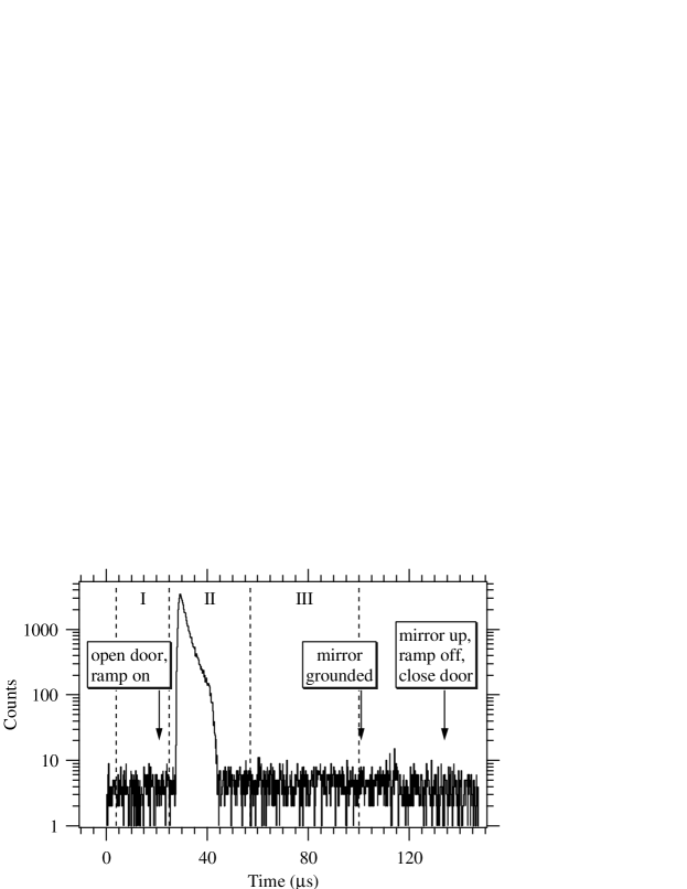
Figure 23: A typical plot of proton detection time after gating on the detector ($t=0$). Regions I and III are used to subtract background from the peak region II. After correcting for deadtime in the time-to-digital converter, the resulting peak area gives the proton rate $\dot{N_{p}}$.

Protons that were born in the trap (grounded electrode region) were trapped with 100% efficiency. However protons that were born near the door and mirror (the “end regions”), where the electrostatic potential is elevated, were not all trapped. A proton born in the end region was trapped if its initial (at birth) sum of electrostatic potential energy and axial kinetic energy was less than the maximum end potential. This complication caused the effective length $L$ of the trap to be difficult to determine precisely. It is for this reason that we varied the trap length. The shape of the electrostatic potential near the door and mirror was the same for all traps with 3–10 grounded electrodes, so the effective length of the end regions, while unknown, was in principle constant. The length of the trap can then be written $L=nl+L_{\rm end}$ where $n$ is the number of grounded electrodes and $l$ is the physical length of one electrode plus an adjacent spacer. $L_{\rm end}$ is an effective length of the two end regions; it is proportional to the physical length of the end regions and the probability that protons born there will be trapped. From Eq. (121) and (122) we see that the ratio of proton counting rate to alpha counting rate is then

$$\frac{\dot{N_{p}}}{\dot{N}_{\alpha}}=\tau_{n}^{-1}\left(\frac{\epsilon_{p}}{\epsilon_{0}v_{o}}\right)(nl+L_{\rm end}).$$ (123)

We fit $\dot{N_{p}}/\dot{N_{\alpha}}$ as a function of $n$ to a straight line and determine $\tau_{n}$ from the slope, so there is no need to know the value of $L_{\rm end}$, provided that it was the same for all trap lengths. Figure 24 shows raw data from a typical run, proton count rate vs. trap length $n$.

Figure 24: Typical raw proton count rate $\dot{N_{p}}$ vs. trap length data, fit to a straight line (top), and residuals (bottom). These data have not yet been corrected for nonlinearities.

Because of the symmetry in the Penning trap’s design, $L_{\rm end}$ was approximately equal for all trap lengths that we used. However there were two trap-length-dependent effects that broke the symmetry: the gradient in the axial magnetic field, and the divergence of the neutron beam. Each of these effects caused $L_{\rm end}$ to vary slightly with trap length. A detailed Monte Carlo simulation of the experiment, based on the measured and calculated magnetic and electric field inside the trap, was developed in order to correct for these trap nonlinearities. It gave a trap-length dependent correction that lowered the lifetime by 5.3s.

Surface barrier (SB) and passivated ion-implanted planar silicon (PIPS) detectors were used at various times for counting the protons. The proton detectors were large enough so that all protons produced by neutron decay in the collimated beam, defined by C1 and C2, would strike the 19.7-mm diameter active region after the trap was opened. The detector was optically aligned to the magnetic field axis, and the alignment was verified by scanning with a low energy electron source at the trap’s center and with actual neutron decay protons. When a proton hit the active region of the detector, the efficiency for proton detection was less than unity because: 1) a proton can lose so much energy in the inactive surface dead layer that it deposits insufficient energy in the active region to be detected; 2) a proton can be stopped within the dead layer and never reach the active region; 3) a proton can backscatter from the dead layer or the active region and deposit insufficient energy. In the first two cases, the proton will definitely not be detected. We denote the fraction of protons lost in this manner by $f_{\rm Lost}$. In the last case, there is some probability that the backscattered proton will be reflected back to the detector by the electric field and subsequently be detected. We denote the fraction of protons that backscatter but still have some chance for detection by $f_{\rm Bsc}$.

To determine the proton detection efficiency, we ran the experiment with a variety of detectors with different dead layer thicknesses and different acceleration potentials. The fraction of protons lost $f_{\rm Lost}$ and the fraction that backscatter $f_{\rm Bsc}$ were calculated using the SRIM 2000 Monte Carlo program ZIE00 . We found that $f_{\rm Lost}$ varied from $4.0(3)\times 10^{-5}$ to $8.0(6)\times 10^{-3}$, and $f_{\rm Bsc}$ from $1.83(13)\times 10^{-3}$ to $2.37(17)\times 10^{-2}$, depending on the detector and acceleration potential. The proton counting rate $\dot{N_{p}}$ for each run was multiplied by $1+f_{\rm Lost}$ to correct for lost protons. The correction for backscattered protons was not as simple because of the unknown probability for a backscattered proton to return and be detected, so we made an extrapolation of the measured neutron lifetime to zero backscatter fraction (see Figure 25).

The neutron detector target was a thin (0.34 mm), 50-mm-diameter single crystal wafer of silicon coated with a 38 mm diameter deposit of ⁶LiF, fabricated at the Institute for Reference Materials and Measurements (IRMM) in Geel, Belgium. The manufacture of deposits and characterization of the ⁶LiF areal density were exhaustively detailed in measurements performed over several years TAG91 . The average areal density was $\rho=(39.30\pm 0.10)~{}\mu\rm{g/cm^{2}}$. The $\alpha$ particles and tritons produced by the the ${}^{6}{\rm Li}(n,t)^{4}$He reaction were detected by four surface barrier detectors, each with a well-defined and carefully measured solid angle. The geometry was chosen to make the solid angle subtended by the detectors insensitive to first order in the source position. The parameter $\epsilon_{0}$ gives the ratio of detected alphas/tritons to incident thermal neutrons. It was calculated using

$$\epsilon_{0}=\frac{\sigma_{0}}{4\pi}\int\int\Omega(x,y)\rho(x,y)\theta(x,y)dxdy,$$ (124)

where $\sigma_{0}$ is the cross section at thermal ($v_{0}=2200$ m/s) velocity, $\Omega(x,y)$ is the detector solid angle, $\rho(x,y)$ is the areal mass density of the deposit, and $\theta(x,y)$ is the areal distribution of the neutron intensity on the target. The ⁶Li thermal cross section is ($941.0\pm 1.3$) b  CAR93 . It is important to note that we take the ENDF/B-6 $1\sigma$ uncertainty from the evaluation, not the expanded uncertainty, to be the most appropriate for use with this precision experiment. The neutron detector solid angle was measured in two independent ways: mechanical contact metrology and calibration with ²³⁹Pu alpha source of known absolute activity. These two methods agreed to within 0.1 %.

Proton and neutron counting data were collected for 13 run series, each with a different proton detector and acceleration potential. The corrected value of the neutron lifetime for each series was calculated and plotted vs. backscattering fraction, as shown in Figure 25. A linear extrapolation to zero backscattering gave a result of $\tau_{n}=(886.8\pm 1.2{\rm[stat]}\pm 3.2{\rm[sys]})$ s. Our result would be improved by an independent absolute calibration of the neutron counter, which would significantly reduce the two largest systematic uncertainties, in the ⁶LiF foil density and ⁶Li cross section. A cryogenic neutron radiometer that promises to be capable of such a calibration at the 0.1% level has recently been demonstrated Zema, and we are pursuing this method further. With this calibration, we expect that our experiment will ultimately achieve an uncertainty of less than 2 seconds in the neutron lifetime.

We thank P. Robouch of the IRMM for assistance in the characterization of the ⁶LiF and ¹⁰B targets. We also thank J. Adams, J. Byrne, A. Carlson, Z. Chowdhuri, P. Dawber, C. Evans, G. Lamaze, and R. D. Scott for their very helpful contributions, discussions, and continued interest in this experiment. We gratefully acknowledge the support of NIST (U.S. Department of Commerce), the U.S. Department of Energy (interagency agreement No. DE-AI02-93ER40784) and the National Science Foundation (PHY-9602872).

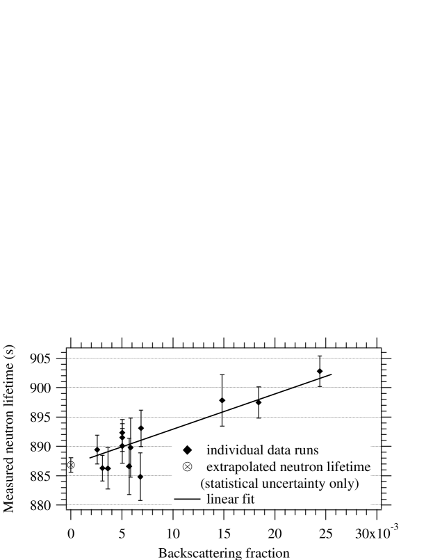
Figure 25: A linear fit of the measured neutron lifetime at varying values of the detector backscattering fraction. The extrapolation to zero backscattering gives the free neutron lifetime.

*A Magnetic Trap for Neutron-Lifetime Measurements
A Magnetic Trap for Neutron-Lifetime Measurements F.J. Hartmann for the UCN-group: I. AltarevA. FreiF.J. HartmannS. PaulG. PetzoldtR. PickerW. SchottD. TortorellaU. TrinksO. Zimmer

49 Introduction

Two important weak-interaction parameters may be determined from the $\beta$-decay of the free neutron: the absolute value of the matrix element $V_{\mathrm{ud}}$ and the ratio $\lambda=g_{\mathrm{A}}/g_{\mathrm{V}}$ of the axial-vector and vector coupling constants Abe00 . Here the knowledge of the neutron lifetime $\tau_{\mathrm{n}}$ and one parameter of the correlation between neutron direction or spin and direction and/or spin of the decay products is sufficient.

Table 8: Experimental results for the neutron lifetime $\tau_{\mathrm{n}}$.

Method	$\tau_{\mathrm{n}}$ (s)			Authors
Storage ring & counters	877	$\pm$	10	Paul et al. Pau89
Gravitational trap & counter	887.6	$\pm$	3.0	Mampe et al. Mam89
Gravitational trap & counter	888.4	$\pm$	3.1 (stat.)	Nezvishevski et al. Nes92
			1.1 (syst.)
Gravitational trap & counter	882.6	$\pm$	2.7	Mampe et al. Mam93
Penning trap for $p$&counter	889.2	$\pm$	3.0 (stat.)	Byrne et al. Byr96
			3.8 (syst.)
Gravitational trap & counter	885.4	$\pm$	0.9 (stat.)	Arzumanov et al. Arz00
			0.4 (syst.)
Gravitational trap & counter	881	$\pm$	3	Pichlmaier et al. Pic00
Mean value	885.7	$\pm$	0.8	Particle Data GroupPDG02hart

The most recent measurements of $\tau_{\mathrm{n}}$ were performed by storing ultra-cold neutrons (UCN) in material and gravitational traps and measuring the number of surviving neutrons as a function of time. Table 8 shows the results of the lifetime experiments with $\sigma(\tau_{\mathrm{n}})\leq 10$ s.

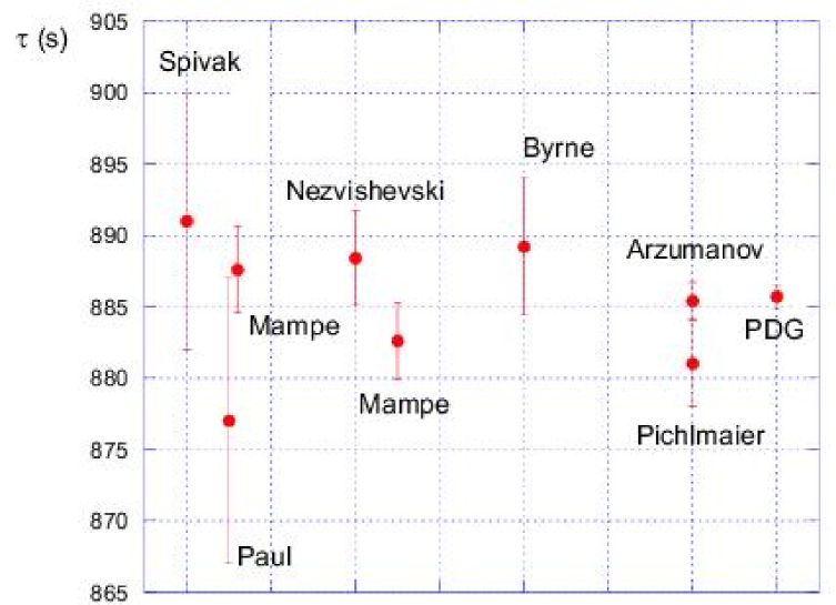
Figure 26: Neutron-lifetime measurements with $\sigma(\tau_{\mathrm{n}})\leq 10$ s

.

The value for $\tau_{\mathrm{n}}$ adopted by the Particle Data Group PDG02hart is mainly determined by one measurement Arz00 . As may be seen from Fig. 26, the results from different groups scatter appreciably. This may be due to the fact that the UCN stored in the trap hit the walls many times during the measuring period and even a very low loss probability per wall collision leads to an appreciable decrease in the measured neutron lifetime. The nature of these losses at the trap walls is not completely clarified up to now and systematic errors may show up during the necessary extrapolation to infinite trap volume. Arzumanov et al. themselves state in their latest publication: ”The major problem … is caused by losses of UCN in collisions with the trap walls”. Magnetic trapping avoids neutron contact with the trap walls and stays free of the systematic uncertainties connected with this source of losses. Hence experiments with magnetic traps are complementary to the common method and a welcome addition.

As early as in 1951 W. Paul Pau51 proposed to store neutrons in magnetic traps. The method is based on the interaction of the neutron magnetic moment $\mu_{n}$ with an inhomogeneous magnetic field. Neutrons with the right orientation of their magnetic moment, the low-field seekers, are driven away from the regions of large magnetic fields at the trap walls. The neutron-spin projection on the magnetic field is an adiabatic constant: for sufficiently slow change of the direction of the magnetic field the spin turns with the field and no spin flip occurs. The angular velocity of the rotation of the field lines seen by the neutron has to be small compared with the frequency of the neutron Larmor precession in the field, $\omega_{\mathrm{Larmor}}=|\gamma|\cdot B$ (with the gyromagnetic ratio $\gamma=183$ MHz/Tesla).

50 Experimental arrangement

50.1 Layout of the experimental set-up

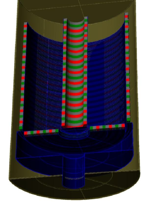
Figure 27: Schematic view of the magnetic storage device for UCN. The superconducting coils are shown in red and green, the soft iron layers in grey and the neutron reflectors and guides in blue.

A schematic view of the planned trap with superconducting magnets is shown in Fig. 2. A torus with 10 cm inner and about 50 cm outer radius and with a height of around 1.2 m is composed of sandwiches of superconducting ring coils with rings of permendur (a NbFeV alloy) or soft iron in between. The bottom of the trap is put together from concentric rings, again from soft ferromagnetic material between superconducting coils. The axis of the torus stands vertical and the top remains open. A field at the walls of about 2 Tesla is sufficient to confine UCN with energies below 120 neV. Gravitation prevents these UCN from leaving through the top. Two ring-shaped slits in the bottom allow filling the trap and detecting depolarized neutrons. In order to fill the bottle one (or several) coils around the slits are switched off.

The probability $w$ for non-adiabatic reorientation during passage through regions of low magnetic field is given by Vla61

$$w=\exp\left(-\frac{\mu\cdot B_{\mathrm{min}}^{2}}{\hbar\cdot|\mathrm{d}B/\mathrm{d}t|}\right)=\exp\left(-\alpha\right)$$

Spin-flip in the low-field region inside the torus is avoided by installing a straight bar in the torus axis and letting a current of about 100 A flow. This keeps the magnetic field everywhere inside the trap larger than 0.2 mTesla and - at velocities below 5 m/s - makes $\alpha$ stay well above one thousand.

At a volume of about 900 dm³ and a UCN density of about 10/cm³ at the high-flux reactor of Institut Laue-Langevin in Grenoble we may expect to store more than $10^{6}$ UCN with the right orientation of the magnetic moment in one filling.

50.2 Experimental procedure

In order to fill the UCN storage unit the trap is operated with a weak magnetic field in the outer slit. To this end the coils at the lower, outer edge (cf. Fig. 2 are switched off. After filling with neutrons of one spin direction the entrance slit is closed by a shutter covered with Be or ⁵⁸Ni. Now the current in the coils is increased again, slow enough to leave the current in the other coils nearly unaffected. Afterwards the shutter may be opened again.Under these circumstances the time constant for filling through a 3-5 cm slit is as low as about 10 s.

After trapping the neutrons we can determine their number as a function of time. Three methods seem feasible

1. At different times after filling a UCN detector is lowered into the trap and counts the number of neutrons left at that moment. This is possible as there are no coils at the top of the trap. Semiconductor detectors with very low reflectivity (and correspondingly high efficiency) for UCN have been developed at our institute. The detector itself is covered by a thin multilayer of ⁶LiF and ⁶²Ni Pet01 . This guarantees a negative Fermi potential down to lowest energies and efficient detection of the products from the reaction

   $$n+\mathrm{{}^{6}Li}\Rightarrow\mathrm{{}^{3}H}+\mathrm{{}^{4}He}.$$

   Another possibility would be the use of a mixture of ⁶LiF and ⁷LiF. The isotopic composition has then to be adjusted to reach negative Fermi potential. The preparation of the UCN detector would become much simpler if one could - as has also been proposed - use a thin backing for the neutron-sensitive layer and thus separate it from the detector.

2. Again at different times after filling the current in dedicated superconducting coils is ramped down and the neutrons flowing through the entrance/exit slit are registered by a UCN detector below the trap. In this case a ³He counter may be used as the UCN are accelerated by gravity.

3. The protons from neutron decay are accelerated towards the top of the setup by an electric field generated via field wires at the torus walls. A voltage of about 5 kV between bottom and top seems sufficient. According to calculations more than 90% of the protons reach the top of the torus; this because part of them are reflected in the magnetic field near the walls. After further acceleration to about 30 keV these protons hit a thin foil of large area from a suitable material (e.g. kapton with a thin Al layer). The electrons from ion-induced electron emission are accelerated towards an (again large) scintillator that is held at zero potential. The (weak) scintillation light is detected with sensitive photomultipliers or hybrid photomultiplier tubes. Several other schemes of proton detection are considered at the moment, but it is not yet clear, how feasible they are.

50.3 Possible systematic errors and their evaluation

Important sources of systematic errors are i) the presence of neutrons of wrong polarization (high-field seekers) at measurement start and ii) neutron spin flip during the measuring cycle. In both cases neutrons may escape from the storage volume and are lost. In order to detect them, the walls of the trap will be covered by beryllium or DLC (diamond-like carbon). Thus these neutrons are reflected at the walls and finally reach the bottom of the trap, where they leave it through the slits and are detected. Monte-Carlo calculations revealed that the time $t_{\mathrm{detect}}$ between spin flip and detection is of the order of 10 s. Figure 3 shows a typical delay-time distribution.

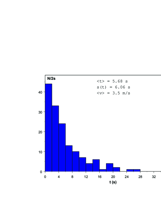
Figure 28: Distribution of the delay times between UCN spin flip and detection of the flipped particles.

The mean value $<t_{\mathrm{detect}}>$ is in good agreement with the value found from the simple formula $t=V/4A\cdot 1/<v>$ that may be derived from kinetic gas theory ($V$ and $A$ are the trap volume and the total area of the exit slit, respectively and $<v>$ is the mean UCN velocity. Figure 4 presents the typical track of a depolarized neutron starting at $r=0.26$ m and $z=0.4$ m; in this case the trap walls are assumed to be at $r=13$ cm and $r=49$ cm.

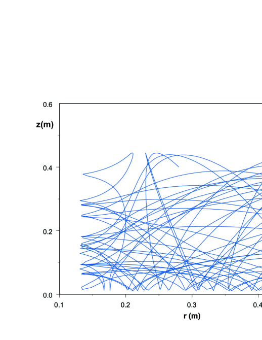
Figure 29: Typical track of a depolarized neutron from the middle of the trap to the exit slit at the lower right corner.

Covering the trap walls with Be has a second advantage. If low-field seeking UCN penetrate through the magnetic wall, they are reflected by Be with very small losses and stay in the storage volume. As the number of such events is expected to be low, losses may be kept negligible.

Another source of systematic errors may be the variation with time of the detection efficiency, e.g. by a change of the neutron density distribution in the storage volume with time. In the case of proton detection it was already pointed out before, that more than 90% of the protons from the inner part of the trap are detected. Hence the effect of efficiency variations should be suppressed. In addition, the other methods for the lifetime evaluation described above may be used for thorough cross-checks.

51 Conclusion and outlook

A trap with superconducting magnets will be built at the Physik-Department of Technische Universität München. The method chosen is complementary to those mainly employed up to now. As the storage volume is large, a large number of neutrons will be available at a time. This makes extensive checks of possible systematic effects possible. Special care will be taken to pin down systematic errors possibly caused by the existence and generation of neutrons with wrong polarization.

The conceptual layout of the magnetic trap is almost ready and construction work will start in 2003.

*Towards a Perfectly Polarized Neutron Beam Towards a Perfectly Polarized Neutron Beam A. Petoukhov, T. Soldner, V. Nesvizhevsky, M. Kreuz, M. Dehn,
M. Brehm A. Petoukhov, T. Soldner, V. Nesvizhevsky, M. Kreuz, M. Dehn,
M. Brehm

52 Motivation

Many experiments in particle physics with cold neutrons require both, a high degree of neutron polarization and its precise measurement. The neutron polarization enters linearly in the measurements of beta and antineutrino asymmetry in neutron beta decay. Improvements of these experiments are particularly important to test the unitarity of the CKM matrix and to search for right handed currents. Their next generation aims to push the precision below 0.1%. This requires corresponding precision of polarization. Other types of experiments require a neutron beam with a very homogeneous and wavelength independent polarization with variation of less than 10^-3 (whereas the absolute value is less important here). Examples are spin rotation experiments that search for parity or time reversal violation in the passage of polarized neutrons through matter.

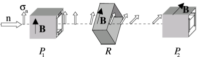
Figure 30: Scheme of double SM polarizers in crossed geometry.

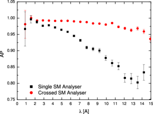
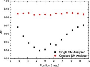
Figure 31: Comparison of single analysed and double SM analysed in crossed geometry: (Top) wavelength, (Bottom) angular dependence.

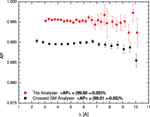
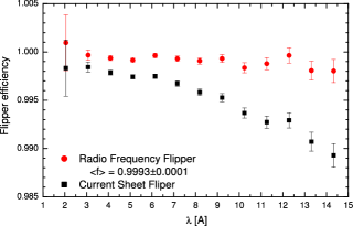
Figure 32: Comparison of (Top) double SM analysed in crossed geometry and ³He spin filter, (Bottom) radio frequency and current sheet spin flipper.

53 Status of cold neutron beam polarization techniques

Presently, super mirror (SM) polarizers schaerpf1989 ; schaerpf1989a are the most powerful tool to polarize a white neutron beam. The polarization resulting from spin dependent reflections on magnetized SMs depends on the wavelength and the incident angle. Using this technique, a neutron beam with a polarized intensity of $2\cdot 10^{9}$ n/cm²s and an averaged polarization of 98.5% is available at PF1b (Institut Laue Langevin). However, the variation of the polarization in the beam due to wavelength and position can be as high as 20% and 3%, respectively (see Fig. 31). This strong variation limits the application of SM polarizers in spin rotation experiments since a change of position or orientation of the sample changes the effective neutron polarization.

In polarization analysis, only the convolution of polarizing and analyzing power can be determined. Therefore, for an absolute measurement of the beam polarization - as required by neutron beta decay experiments - the analyzing power has to be known independently. This is not possible with SM analysers but can be solved using opaque ³He spin filters zimmer1999 ; zimmer1999a . This technique provides 100% analyzing power and is not angle and spatial dependent. It can therefore be used to average over the neutron beam (with several practical problems like corrections for windows, the time dependence of ³He polarization, etc.). However, it is limited to a narrow wavelength range by a very low and wavelength dependent transmission of less than $10^{-3}$. Moreover, for an inhomogeneous beam, even the correct average polarization may differ from the average seen from the experimental set-up.

A perfectly polarized neutron beam should therefore be homogeneous on the level of the attempted experimental precision. Today, this can be obtained neither with a single SM nor with a ³He polarizer.

54 The crossed geometry of two SM polarizers

We propose to use double SM polarizers in crossed geometry (Fig. 30). This geometry is particularly important since the angular acceptance of one device is independent of the angular acceptance of the other. Therefore, both devices are independent. This allows to predict the properties of the combined polarizer (polarization $P_{12}$ and transmission $T_{12}$) from the properties of the single devices ($P_{i}$ and $T_{i}$) using the standard matrix formalism:

$$P_{12}=\frac{P_{1}+P_{2}}{1+P_{1}P_{2}}\approx 1-\frac{1}{2}(1-P_{1})(1-P_{2})$$ (125)

and

$$T_{12}=T_{1}T_{2}.$$ (126)

Using typical SM polarizer properties ($P_{i}\approx 98$%), we predict a very high polarization ($P_{12}>99.9$%) for a wide wavelength range and an angular variation of less then 10^-3. The intensity should drop only to about 50% of the single device ($T_{1},T_{2}\approx 50$% for the “good” spin component).

55 Experimental tests

For the experimental tests at PF1b the following set-up was used: The polarized beam was created by double SM polarizers in crossed geometry, followed by a radio frequency flipper ($f=50$ kHz) and a current sheet flipper. The beam was analysed by either a single SM analyzer, double SM analysers in crossed geometry, or a polarized ³He spin filter. A time of flight set-up allowed a wavelength-resolved analysis. All SMs were adjusted to maximum transmission. To cover the wavelength range between 3 and 10 Å, different ³He cells and pressures were used.

Fig. 31a (31b) compares the wavelength (angular) dependence of the product AP of polarization and analyzing power for the single and the crossed analysed. Both dependencies are suppressed strongly for the crossed geometry.

In Fig. 32b the performances of the two flippers are compared. The efficiency of the radio frequency flipper was 99.93(1)%, averaged between 2 and 15 Å (only statistical error given).

Fig. 32a compares the AP products obtained with the crossed analysed and with the ³He spin filters. The values 99.01(5)% and 99.60(5)% differ significantly. We explain this by a depolarization in the SM analysed itself and attribute the difference between 99.60(5)% and 100% to a depolarization in the SM polarizer. A depolarization during the polarization transport can be excluded since we use the same configuration and change only the analysed. Moreover, any depolarization due to a non-adiabatic transport in the magnetic field should be wavelength dependent. This was not observed within the obtained precision of 10^-3. To check the depolarization, we reduced the SM housing magnetic field from 35 mT to 20 mT in both, polarizer and analysed. The AP product dropped by 1%.

56 Conclusions

For absolute measurements of correlations in neutron beta decay and for spin rotation experiments, double SM polarizers in crossed geometry should be used to polarize the beam. For this set-up, an average polarization of more than 99.5% can be obtained for a cold neutron beam. Spatial and wavelength dependencies can be neglected on the 0.1% level. The neutron flux is reduced by about 50% only compared to a single SM polarizer. For such a perfect beam the polarization can be measured with a precision of better than 0.1% using ³He spin filters. A spin flip efficiency of more than 99.9% can be reached with a radio frequency spin flipper. We hope that the absolute value of polarization can be increased in the near future using higher SM housing magnetic fields.

Part II

missing

*Order-$\alpha$ Radiative Corrections to Neutron, Pion and Allowed Nuclear $\beta$-Decays Order-$\alpha$ Radiative Corrections to Neutron, Pion and Allowed Nuclear $\beta$-Decays

F. Glück

57 Introduction

The theoretical analysis of neutron decay is more reliable than the analysis of high energy beta decays. There are several simplifications here:

1. the $q^{2}$ dependence of the form factors is negligible;

2. the effect of the vector form factor $f_{3}$ and the $g_{2}$ and $g_{3}$ axialvector form factors is negligible;

3. the value of the weak magnetism form factor $f_{2}$ is predicted by the conserved vector current hypothesis (CVC); this is tested by nuclear beta decays;

4. we have $f_{1}(0)=1$ to high precision: this follows from the Behrends-Sirlin-Ademollo-Gatto theorem, and also from quark model computations.

After these simplifications we have only 2 free parameters: the $up-down$ element $V_{ud}$ of the CKM-matrix, and the $\lambda=g_{1}(0)$ axialvector form factor.

In the 3-body pion beta decay $\pi^{\pm}\to\pi^{0}e^{\pm}\nu_{e}$ the $q^{2}$ dependence is larger, but here an additional simplification is the absence of the axialvector form factors.

In the case of the nuclear beta decays the theoretical analysis is not so simple and reliable, due to the isospin-symmetry breaking (charge dependent) corrections to the matrix elements, and the larger recoil corrections in beta decays with higher decay energies. Nevertheless, good nuclear structure models are available nowadays which can be employed to compute these corrections to the required precision.

Low energy beta decays can be used to test some important aspects of the Standard Model (SM): the unitarity of the CKM-matrix, the absence of the right-handed, scalar, tensor and time-reversal violating weak couplings. It is obvious now that any deviation from the SM should be quite small. Therefore, very accurate measurements are needed in order to test precisely these deviations, and they require precise theoretical analysis.

One of the most important small corrections to the theoretical distributions and quantities are the radiative corrections. These corrections are the consequences of the presence of photons which are created by the charged particles of the beta decay processes. These photons can change slightly the various decay probabilities, but some of them (the bremsstrahlung photons, which are in principle detectable) can also change the kinematics of the decay processes. These small changes are important in the analysis of the precision experiments. For example: neglecting these corrections one could see some deviations from the Standard Model which in reality is not present. An incomplete theoretical analysis could result in a false interpretation of an experiment which has otherwise no serious systematic errors.

58 Bremsstrahlung and virtual photons

The radiative corrections are the consequences of the interaction of photons with charged particles. We know from classical electrodynamics that accelerating particles create electromagnetic field, and we know from quantum physics that this field is quantized, with the photons representing its quantums. During beta decay charged particles come into existence with large velocities, and this mechanism creates photons.

It is important to distinguish 2 different types of photons: bremsstrahlung and virtual. The bremsstrahlung photons are on-shell, that is for them $E=|{\bf p}|$ (with the $c=1$ particle physics convention), where $E$ is their energy, and ${\bf p}$ denotes their three-momentum. In some sense, these bremsstrahlung photons are real: they can go very far from the beta decay region, so they are in principle detectable; although, most of these photons have very small energy, so it is not easy to detect them.

On the other hand, the virtual photons are off-shell: for them $E\not=|{\bf p}|$, they behave so as if they had a non-zero mass. These virtual photons can live only for an extremely short time and within a very small region of space: they are constrained to the space-time vicinity of the beta decay process.

The contribution of the bremsstrahlung photon events is represented by Feynman diagrams where the photon is created in a vertex on a charged particle line, and it goes out into infinity. On the other hand, the virtual photon contributions are visualized by diagrams where the photon is created in a vertex point on a charged particle line, and it is absorbed in another vertex point on the same charged particle line (self-energy diagrams) or another line (box or vertex diagrams).

The various measurable quantities of the beta decays can be calculated from the decay amplitude by using the diagrams of the decay processes and the Feynman rules of the Standard Model. Let ${\cal M}_{0}$ denote the decay amplitude without radiative corrections; we call this zeroth-order amplitude. The zeroth-order part of the measurable quantities are calculated from $|{\cal M}_{0}|^{2}$ by summation and averaging over the spins and by phase-space integration over the momenta of the particles participating in the beta decay. The ${\cal M}_{VIRT}$ virtual photon amplitude has to be added to the zeroth-order one, since the decay process with virtual photon is quantum mechanically indistinguishable from the decay events without photon. On the other hand, the bremsstrahlung process could be, in principle, distinguished from the zeroth-order process, therefore the ${\cal M}_{BR}$ amplitude should not be added to ${\cal M}_{0}$, but the bremsstrahlung parts of the measurable quantities should be computed by phase-space integration and spin summation of $|{\cal M}_{BR}|^{2}$.

59 Photon bremsstrahlung

According to the Bloch-Nordsieck theorem BlochNordsieck , bremsstrahlung photons are always present in processes where charged particles are involved. With some finite energy resolution of the detection system only the bremsstrahlung events with $K>K_{min}$ photon energy can be distinguished from the no-photon decay events. Assuming $K_{min}\sim 1keV$ resolution energy, in neutron decay the probabilities to get 1 and 2 photons during a decay event are: ${\cal P}(1\gamma)\sim 0.5\%$ and ${\cal P}(2\gamma)\sim 0.001\%$, respectively. Therefore, it is usually enough to calculate the one-photon bremsstrahlung.

The photons created during the beta decay process are called internal brems-strahlung photons. They should be distinguished from the external brems-strahlung photons: the latter are created during a collision process of beta electrons with external nuclei which are far from the beta decay point. Therefore external bremsstrahlung is completely different from internal bremsstrahlung.

The internal bremsstrahlung amplitude can be written as a sum of leptonic and hadronic parts:

$${\cal M}_{BR}={\cal M}_{l}+{\cal M}_{h},$$ (127)

where the ${\cal M}_{l}$ and ${\cal M}_{h}$ amplitudes represent the diagrams with the photon emitted by the charged lepton (here electron) and the hadrons, respectively. The calculation of the ${\cal M}_{l}$ part is simply QED, so it is always reliable. The ${\cal M}_{h}$ hadronic part contains strong interaction effects, so for energetic beta decays it is not easy to calculate reliably. This could be, however, an advantage since for example by the measurement of the radiative pion decay $\pi\to e\bar{\nu}\gamma$ one can obtain important information about the strong interaction, and it is possible also to restrict the weak tensor coupling constant. We mention that in radiative pion and kaon decays the ${\cal M}_{l}$ amplitude together with the point-like hadron model approximation part of ${\cal M}_{h}$ is usually called inner bremsstrahlung (IB), and the remaining is called structure-dependent contribution (SD) (see Ref. Bryman , page 166).

In the case of the beta decays with small decay energy, like neutron, $\pi_{e3}$ and nuclear beta decays, the situation is different. For example, in neutron decay the maximum photon energy allowed by kinematics is $K_{max}=0.78MeV$. We know since Yukawa that about 140 MeV energy corresponds to 1 fermi wavelength, so in our case the minimum wavelength of the bremsstrahlung photon is much more larger than the dimension of the nucleons:

$$\lambda_{min}^{(\gamma)}\gg\,1fm.$$ (128)

Obviously, these large wavelength photons cannot penetrate inside the nucleons, they can see mainly their charges (and to some extent their magnetic moment). The photon bremsstrahlung calculation of beta decays with small decay energy is almost model independent, therefore very reliable.

We can see also to what extent is this photon bremsstrahlung calculation model independent. For very small energy photon the hadronic bremsstrahlung amplitude is proportional to the zeroth order amplitude:

$${\cal M}_{h}[small\;K]\approx e\frac{(p\varepsilon)}{(pk)}{\cal M}_{0}$$ (129)

where $k=(K,{\bf k})$ denotes the photon four-momentum ($K$ is the photon energy) , $\varepsilon$ its polarization vector, and $e$ is the electron charge. We see that for small photon energy the bremsstrahlung amplitude is proportional to $K^{-1}$. After phase space integration one can see that the bremsstrahlung photon spectrum has also an order-$K^{-1}$ behavior for small $K$ (see Schopper , pages 76-84). The coefficient of the $K^{-1}$-term, which is dominant for low photon energy, is model independent. Due to the Low-theorem (see Refs. Low ; Adler ; Burnett ; Fearing ), which is a consequence of the gauge invariance of QED, not only the order-$K^{-1}$ , but also the order-$K^{0}$ part of ${\cal M}_{h}$ can be calculated model independently, using the zeroth-order amplitude and the electromagnetic form factors of the hadrons involved in the beta decay (an application of the Low-theorem to hyperon semileptonic decays can be found in Ref. Gluck97a ). Thus only the order-$K$ part (together with higher orders) of the hadronic bremsstrahlung amplitude is model dependent. Compared to the dominant order-$K^{-1}$ part this is of order $(K/m_{n})^{2}\sim 10^{-6}$ for neutron decay. We can then conclude:

It is not possible to obtain any strong interaction dynamical information from photon bremsstrahlung measurement in neutron decay. The bremsstrahlung here is completely determined by QED.

For 3-body pion and for allowed nuclear beta decays the above factor is larger than $10^{-6}$, but is seems very unlikely that any structure dependent part of the photon bremsstrahlung could be measured in these decays.

The photon bremsstrahlung calculation is theoretically simple and reliable. On the other hand, technically it is more complicated. In order to compute the measurable quantities, one has to evaluate many-dimensional integrals like

$$\int\frac{d^{3}{\bf p}_{p}}{E_{p}}\int\frac{d^{3}{\bf p}_{e}}{E_{e}}\int\frac{d^{3}{\bf p}_{\nu}}{E_{\nu}}\int\frac{d^{3}{\bf k}}{K}\delta^{4}(p_{n}-p_{p}-p_{e}-p_{\nu}-k)\sum_{spin}|{\cal M}_{BR}|^{2}.$$ (130)

The $|{\cal M}_{BR}|^{2}$ expression can be evaluated by symbolic algebra programs (like REDUCE). One has to use Dirac matrix algebra, and Lorentz-index summation have to be performed. These symbolic formulae can be checked by numerical calculation of the amplitude.

For the integration, there exist 2 different methods. First, it is possible to use semianalytical integration (see Refs. Gluck90 ; Gluck92 ). This gives very precise results, but the calculation of many complicated analytical integrals is rather difficult. A more simpler method is with Monte Carlo integration. In this case the computer evaluates the complicated integrals, much more smaller amount of human effort is necessary with this method. The accuracy is limited by statistics, but there is no problem to generate $10^{6}$ events, and this gives already the accuracy needed for meaningful results. The method is very flexible: the same computer program can be used in order to calculate radiative correction to any kind of measurable quantity. The method is especially suitable for experimental off-line data analysis, where the various kinematic cuts, detection efficiencies etc. require complicated modifications of the theoretical distributions. Using the Monte Carlo method one can also perform weighted or unweighted event generations.

The $|{\cal M}_{BR}|^{2}$ integrand has large peaks for small photon energy ($K\to 0$: infrared peak), and in the case of larger decay energies for almost parallel photon and electron momenta (collinear peak). These peaks make the simple Monte Carlo integration inefficient (one has to generate very large number of events). This problem can be completely solved by importance sampling: one has to generate more events in the phase space region where the integrand is large (see Refs. Gluck96 ; Gluck97a ; Gluck97b for different importance sampling solutions).

In order to calculate radiative correction to some quantity, one has to include also the very small energy photons into the integration region. But going with the $K$ photon energy to zero, the integral goes logarithmically to infinity (we have seen above that the bremsstrahlung photon spectrum behaves as $K^{-1}$ for small $K$). This infrared divergence problem can be solved by regularization. One kind of regularization is the following: a small photon mass $m_{\gamma}$ is introduced in the photon four-momentum formulae, and then the integrals become finite, namely $\ln m_{\gamma}$ terms appear after integration. The same photon mass regularization has to be performed for the calculations of the virtual photon contributions, too. The virtual correction results also contain $\ln m_{\gamma}$ terms, but with opposite sign and same magnitude as the bremsstrahlung corrections. In the sum of the bremsstrahlung and virtual corrections the photon mass term disappears: the complete radiative correction is free from infrared divergence!

If the Monte Carlo method is employed for the radiative correction computation, an expedient method is the following: the photon bremsstrahlung integration is divided into soft and hard regions. In the soft region the photon energy is small, smaller than some given $\omega$ soft-photon cutoff value; we can use here 3-body decay kinematics, the integrals containing the regulator photon mass can be calculated rather simply analytically. Adding this contribution to the virtual part, the photon mass logarithm disappears, and we get the virtual-soft part of the radiative correction. In the hard region the photon energy is larger than the $\omega$ cutoff, we use here 4-body kinematics, but the photon mass can be put equal to zero in these integrals (this makes the importance sampling method easier to apply).

The hard bremsstrahlung photons change the beta decay kinematics. It is important to take into account this fact, in order to obtain meaningful radiative corrections results

In Refs. YM76 ; GM78 analytical formulae were published for the radiative correction to the electron and neutrino asymmetry and the electron-neutrino correlation of nuclear and neutron beta decays. Their result is, however, not applicable for the precise analysis of the measurements. The reason is the following. During the radiative correction calculation, one has to take into account the bremsstrahlung photons, which arise in the beta decay with small, but non-negligible probability, together with the electron and antineutrino. These photons change considerably the decay kinematics. If one calculates the radiative correction to the neutrino asymmetry and the electron-neutrino correlation with electron and proton detection, first the electron and proton momenta have to be fixed, and the integrations over the other particle momenta have to be performed with the constraint of the fixed electron and proton momenta. This constraint makes the analytical integrations very difficult. On the other hand, the authors of Refs. GM78 ; YM76 performed the photon bremsstrahlung integration with fixed electron and antineutrino momenta. In this case, the analytical integration is possible. Unfortunately, the proton momentum now changes with the photon momentum during the integration, by momentum conservation. The result of this calculation would be useful only if the antineutrino could be detected and precisely measured. At present, however, this is in neutron and nuclear beta decay measurements impossible.

We mention that the inapplicability of several published radiative correction results for the experimental analysis of semileptonic decay measurements was emphasized already in the eighties Toth84 ; TSM86 (see also Refs. TG89 ; Gluck90 ).

60 Virtual correction and the UV divergence

We have seen that both the bremsstrahlung and the virtual correction have infrared (IR) divergence, so they are separately not observable quantities: only their sum, where the IR divergence disappears, has any meaning to be compared with experimental results.

In addition to IR divergence, the virtual correction has another and more serious divergence: for the calculation of the virtual integrals the virtual photon four-momentum has to be integrated over the whole four-dimensional phase-space region, and this makes the integrals divergent also for large photon energies. The UV divergence is present also in QED virtual integrals, but there it is possible to absorb the UV-divergent parts into the electron mass and charge (renormalization), thus all the UV divergent integrals become finite: we obtain finite radiative correction results. On the other hand, before 1971 nobody was able to find any meaningful renormalization procedure for the weak interactions. All the radiative corrections of the hadronic beta decays contained ultraviolet cutoffs, both in the four-fermion and in the vector-boson theories, and it was not possible to get rid off this cutoff by some renormalization procedure. On the other hand, the order-$\alpha$ correction of the muon decay within the framework of the $V-A$ model was finite, free from the UV-cutoff. In the sixties, after the electromagnetic nucleon form factor measurements of Hofstaedter, several famous physicists (like Feynman, Källen, Berman, Sirlin) conjectured the hypothesis that perhaps the strong interaction could solve this UV divergency problem: for large $q^{2}$ the electromagnetic form factors go rapidly to zero, and this could make the integrals finite. In the middle of the sixties, however, it was obvious due to the current algebra investigations that the strong interaction alone cannot solve the UV divergency problem. It was necessary to develop a renormalizable theory of weak interactions to solve this problem. The $SU(3)_{c}\times SU(2)_{L}\times U(1)$ non-Abelian gauge theory, with spontaneous symmetry breaking due to the Higgs mechanism (Standard Model), was able to provide a renormalizable and phenomenologically realistic model for the weak interaction. It was shown by Sirlin and others in the seventies Lee ; Sirlin74 ; Sirlin78 that the radiative corrections of hadronic beta decays in the framework of the Standard Model are free from ultraviolet divergences.

61 The weak correction

The Feynman diagrams of the order-$\alpha$ virtual corrections can be divided into 2 groups: non-photonic diagrams, with $Z$ and $W$ bosons and Higgs particle in the loops, and photonic diagrams. The photon propagator of the photonic self-energy diagrams can be decomposed as Sirlin74 ; Sirlin78

$$\frac{1}{k^{2}}=\frac{1}{k^{2}-M_{W}^{2}}-\frac{M_{W}^{2}}{k^{2}-M_{W}^{2}}\frac{1}{k^{2}}$$ (131)

Then the whole order-$\alpha$ virtual correction can be separated to weak and photonic parts. The weak part is defined by the non-photonic diagrams, plus the self-energy photonic diagrams taking the first term in the above decomposition. The photonic correction is determined by the photonic box diagram and the self-energy photonic diagrams with the second term in the above decomposition. One can then see that the photonic correction integrals are UV-finite (with the $W$ boson mass as a natural cutoff). The weak correction integrals are not finite, but their UV-divergence disappears after electroweak renormalization, taking also into account the asymptotic freedom of QCD (see Refs. Sirlin74 ; Sirlin78 ).

The final universal result from the weak part of the order-$\alpha$ radiative correction to the decay rate is:

$$r_{weak}=0.02\%$$ (132)

So the many weak diagrams give a very small and fairly reliable correction result. As we will see, the photonic correction is much more larger, and unfortunately it is difficult to calculate reliably (with small theoretical uncertainty), due to some non-perturbative effects.

62 The model independent (outer) photonic correction

The photonic virtual correction has the following general properties: it is UV finite, IR divergent, and depends on strong interaction models.

In the correction calculation the photon energy has to be integrated from zero to infinity. Let us divide the whole integration region into 3 subregions:

1. small: [0,200 MeV]

2. medium: [200 MeV, 4 GeV]

3. asymptotic: [4 GeV,$\infty$]

The region ’small’ contains completely the IR divergence, it is almost free from strong interaction effects, and only this part is sensitive to the momenta and energies of the beta decay particles. It is expedient to separate this part of the correction from the others.

This separation was introduced by Sirlin in 1967 Sirlin67 . He did not use the above arbitrary energy boundary of the region ’small’, but he defined the model independent (MI) virtual correction by using the convective term in the point-like hadron vertex-propagator expression.

Then we use the following definition:

MI radiative correction = MI virtual correction + bremsstrahlung

The MI (model independent) radiative correction has the following important properties:

• It has no strong interaction dependence, so it is reliable;

• It is sensitive to the experimental details
  (e.g.: the photon bremsstrahlung changes the kinematics);

• It changes the spectrum shapes and asymmetries.

Due to these properties, it is important to take into account this correction in precision experimental analysis.

First, this correction changes the beta spectrum shape of beta decays. Sirlin gave a universal analytical formula for the MI correction to the beta spectrum (Eq. 20 in Ref. Sirlin67 . For the case of neutron decay this function is tabulated in Table I of Ref. Gluck93 . One can see that the correction to the shape is about 1 % for neutron decay. For pion beta decay and for allowed nuclear beta decays with higher decay energy this correction is larger. In $E_{e}\to E_{emax}$ limit the correction has a logarithmic singularity, but for beta decays with decay energy below 10 MeV this is practically not relevant. It is important to take into account this correction for accurate weak magnetism, second class form factor, and Fierz term analysis of beta spectrum shapes.

The MI correction to the proton spectrum in neutron decay can be found in Table IV of Ref. Gluck93 . This correction is about 0.1 %, but it changes the $\lambda=G_{A}/G_{V}$ fitted parameter by 0.01 (the ’aspect’ project aims to measure this $\lambda$ by 0.001 precision; see Ref. Zimmerglu ).

The MI radiative correction to the recoil spectrum shapes in ${}^{6}He$ and ${}^{32}Ar$ beta decays was calculated in Ref. Gluck98 . This correction shifts the fitted electron-neutrino correlation parameter $a$ by 0.003; this is approximately the experimental error of the most precise $a$ value measurements of these decays.

It is important to take into account the MI correction also to higher energy beta decays. For example, this correction changes the fitted $\lambda=g_{1}/f_{1}$ ratio in $\Lambda\to pe\nu$ decay by 0.03 (see Ref. Gluck94 ), which is twice larger than the experimental error of the most precise measurement.

The order-$\alpha$ MI corrections to the total decay rates of some beta decays are the following Gluck97b :

• neutron decay: $r_{MI}=$ 1.50 %

• $\pi_{e3}$ decay: $r_{MI}=$ 1.04 %

• $O^{14}\to N^{14}$ decay: $r_{MI}=$ 1.29 %

The order-$\alpha$ MI corrections to the various asymmetry quantities in polarized beta decays are usually rather small (see Refs. Sirlin67 ; Shann ; Yokoo ; Gluck92 ; Gluck96a ; Gluck98a ).

63 The model dependent (inner) photonic correction

While the MI photonic correction can be visualized as integrating the virtual photon in the small energy region, and therefore this correction is sensitive to the external particle momenta, the model dependent (MD) correction gets the main contribution from the large photon energy region, therefore it is not sensitive to the particle momenta. For example, let us assume that a virtual electron with $p_{e}^{\prime}$ momentum emits a virtual photon with four momentum $k$ (this photon is then absorbed by the beta decay hadrons), and it goes into the external electron (momentum: $p_{e}$). From momentum conservation at the electron-photon vertex: $p_{e}^{\prime}=k+p_{e}$. The virtual correction integrand contains the electron propagator depending on the $p_{e}^{\prime}$ virtual electron momentum. If $k$ is large, the small $p_{e}$ momentum can be neglected in $p_{e}^{\prime}$, therefore the integral is practically independent of the external electron momentum $p_{e}$.

We can thus conclude that:

The model dependent correction is not sensitive to the external beta decay particle momenta and to the experimental (kinematical) details.

Sirlin proved in Ref. Sirlin67 the following theorem:

Neglecting terms of order

$$\alpha\frac{E_{e}}{m_{n}}\ln\left(\frac{m_{n}}{E_{e}}\right)\sim 10^{-4}-10^{-5},$$ (133)

the MD correction can be absorbed into the $f_{1}$ vector and $g_{1}$ axialvector form factors.

We can introduce effective form factors:

$$f_{1}^{\prime}=f_{1}\left(1+\frac{\alpha}{2\pi}c\right),\quad g_{1}^{\prime}=g_{1}\left(1+\frac{\alpha}{2\pi}d\right).$$ (134)

The model dependent correction is then defined by 2 numbers: $c$ and $d$. For a given beta decay one can use the same effective form factors for all measurable quantities. The $G_{V}$ weak vector coupling and the $\lambda$ parameters can then be redefined as

$$G_{V}=G_{\mu}V_{ud}f_{1}^{\prime},\quad\lambda=g_{1}^{\prime}/f_{1}^{\prime}$$ (135)

All measurable quantities for a given beta decay depend on the same $G_{V}$ and $\lambda$ parameters. For example, in neutron decay the $\lambda$ parameter can be determined from the electron asymmetry $A$ and from the electron-neutrino correlation parameter $a$. Let us denote these values as $\lambda_{A}$ and $\lambda_{a}$. Within the framework of the Standard Model we need: $\lambda_{A}=\lambda_{a}$. The comparison of these measured parameters provides a sensitive test of the $V-A$ structure of the Standard Model; in the presence of scalar or tensor couplings these parameters should not be necessary equal. What is important here: this test is independent of the model dependent correction; never mind what are the $c$ and $d$ MD corrections, we have to get the same $\lambda$ values for a fixed beta decay type within the SM. Unfortunately, the MD corrections and thus the effective form factors could be different for the different beta decay types (see below).

The $V_{ud}$ element of the CKM matrix can be determined from the measured $G_{V}$ and $G_{\mu}$ couplings, and from the calculated MD correction $c$.

The precise and reliable calculation of the $c$ model dependent correction of the vector coupling is important for the $V_{ud}$ determination, and thus for the CKM unitarity test.

The leading asymptotic behavior in $M_{Z}$ of the order-$\alpha$ radiative correction amplitude to an arbitrary semileptonic decay is given by the universal formula Sirlin82

$${\cal M}_{as}=\frac{\alpha}{\pi}\ln\left(\frac{M_{Z}}{m_{p}}\right){\cal M}_{0},$$ (136)

where $M_{Z}$ and $m_{p}$ are the Z-boson and proton masses.

This part of the model dependent correction depends on the high energy behavior of QCD (asymptotic freedom), so it contains no uncertainties from non-perturbative strong interaction models; it is therefore in fact ’model independent’. The total model dependent correction amplitude can be written as

$${\cal M}_{MD}={\cal M}_{as}+{\cal M}_{med}.$$ (137)

Here the ${\cal M}_{med}$ part comes from the integration over the medium energy range, where the photon energy is around 1 GeV. In this region the virtual photon can have a large effect to the inner structure of the hadrons, therefore this part of the correction depends very much on strong interaction models. Nevertheless, ${\cal M}_{med}$ does not contain any large logarithm, so it is expected that the asymptotic part is dominant.

For total decay rates the asymptotic part gives a correction of

$$r_{as}=\frac{2\alpha}{\pi}\ln\left(\frac{M_{Z}}{m_{p}}\right)=2.1\%$$ (138)

(we have to take the interference between the zeroth order and the virtual amplitudes: $r_{as}=2{\cal R}e({\cal M}_{as}^{*}{\cal M}_{0})/|{\cal M}_{0}|^{2}$). This part of the MD correction is universal: it is the same for all beta decays.

The higher order terms of this asymptotic correction was estimated by Marciano and Sirlin Marciano using renormalization group analysis. The asymptotic correction with the higher order terms is

$$r_{as}^{h.o.}=2.25\%$$ (139)

The medium energy ( non-asymptotic) model dependent correction to the decay rate was estimated also by Marciano and Sirlin Marciano :

$$r_{med}=0.12\pm 0.2\%$$ (140)

(see also Refs. Sirlin78 ; Sirlin95 ; Jaus ; Towner98 ; Towner02 ).

It is unlikely that the real $r_{med}$ correction should be completely different from this result. Nevertheless, this part of the radiative correction is the least reliable, and probably further theoretical investigations are necessary in order to obtain a better understanding of this correction. It should be emphasized also that the $r_{med}$ correction is very likely beta decay type dependent: it is different in neutron decay and in pion beta decay (in the first case, the virtual photon interacts with nucleons, in the second case with pions: these are completely different hadrons).

*Beyond $V_{ud}$ in Neutron Decay
Beyond $V_{ud}$ in Neutron Decay S. Gardner

64 Introduction

Precision studies of nuclear $\beta$-decay have played a crucial role in the rise of Standard Model (SM). More recently, precision studies of neutron $\beta$-decay have been realized as well; the thrust of these efforts has been the determination of the Cabibbo-Kobayashi-Maskawa (CKM) matrix element $V_{ud}$ to realize, in concert with the empirical values of $V_{us}$ and $V_{ub}$, a test of the unitarity of the CKM matrix. The value of $V_{ud}$ is extracted from the vector coupling constant of the nucleon, $f_{1}$, which is determined from the neutron-spin–electron-momentum correlation $A$ and the neutron lifetime $\tau_{n}$.

In this note we consider the systematic determination of all of the couplings of the nucleon weak current, and how such extractions lead to SM tests beyond that of CKM unitarity Zhang . In this context we discuss tests of the conserved-vector-current hypothesis (CVC) feyngm as well as the search for second-class currents (SCC) wein , and, generally, the search for non-V-A currents. In addition, we consider ancillary, low-energy SM tests accessible through neutron radiative $\beta$-decay — and offer perspective on how the low-energy SM tests we enumerate complement experiments at much higher energies.

65 Framework

The differential decay rate for polarized neutron $\beta$-decay in the SM is given by

$$d^{3}\Gamma=\frac{1}{(2\pi)^{5}2m_{B}}(\frac{d^{3}{\mathbf{p}}_{p}}{2E_{p}}\frac{d^{3}{\mathbf{p}}_{e}}{2E_{e}}\frac{d^{3}{\mathbf{p}}_{\nu}}{2E_{\nu}})\delta^{4}(p_{n}-p_{p}-p_{e}-p_{v})\frac{1}{2}\sum_{spins}|{\cal M}|^{2}\,,$$ (141)

where the transition matrix element ${\cal M}$ to leading order in the weak interaction is

$${\cal M}=\frac{G_{F}}{\sqrt{2}}\langle p(p_{p})|J^{\mu}(0)|{\vec{n}}(p_{n},P)\rangle[\bar{u}_{e}(p_{e})\gamma_{\mu}(1+\gamma_{5})u_{\nu}(p_{\nu})]\;,$$ (142)

and the most general form of the hadronic weak current, consistent with its $V-A$ structure, is murph

$$\langle p(p_{p})|J^{\mu}(0)|{\vec{n}(p_{n},P)}\rangle=\bar{u}_{p}(p_{p})(f_{1}(q^{2})\gamma^{\mu}-i\frac{f_{2}(q^{2})}{M_{n}}\sigma^{\mu\nu}q_{\nu}+\frac{f_{3}(q^{2})}{M_{n}}q^{\mu}$$

$$+g_{1}(q^{2})\gamma^{\mu}\gamma_{5}-i\frac{g_{2}(q^{2})}{M_{n}}{\sigma^{\mu\nu}}\gamma_{5}q_{\nu}+\frac{g_{3}(q^{2})}{M_{n}}\gamma_{5}q^{\mu})u_{\vec{n}}(p_{n},P)\,,$$ (143)

where $\sigma^{\mu\nu}=i[\gamma^{\mu},\gamma^{\nu}]/2$, $q\equiv p_{n}-p_{p}$, and $u_{\vec{n}}(p_{n},P)\equiv({1+\gamma_{5}{/\!\!\!\!P}})u_{n}(p_{n})/2$ for a neutron with polarization $P$. Defining $f_{i}\equiv f_{i}(0)$, we adopt the “historic” sign convention $\lambda\equiv g_{1}/f_{1}>0$ for consistency with earlier literature. In the SM, under an assumption of isospin symmetry, we note that $f_{1}=(1+\Delta_{R}^{V})V_{ud}$, where $\Delta_{R}^{V}$ is a small, radiative correction sirlin , the weak magnetism term $f_{2}$ is given by the isovector anomalous magnetic moment, as per the CVC hypothesis gell58 , and both $f_{3}$ and $g_{2}$ are zero. The chiral properties of QCD determine $g_{3}$ in terms of other low-energy constants. Isospin is merely an approximate symmetry, so that $f_{2},f_{3},$ and $g_{2}$ suffer corrections of ${\cal O}(R)$, where $R\approx(M_{n}-M_{p})/\hat{M}$ and $\hat{M}$ is the average neutron-proton mass.

Rewriting the differential decay rate in terms of the correlation coefficients, we find jtw

$$d^{3}\Gamma\propto E_{e}|{p}_{e}|(E_{e}^{\rm max}-E_{e})^{2}$$ (144)

$${}\cdot\Big{[}1+a\frac{{p}_{e}\cdot{p}_{\nu}}{E_{e}E_{\nu}}+{P}\cdot(A\frac{{p}_{e}}{E_{e}}+B\frac{{p}_{\nu}}{E_{\nu}}+D\frac{{p}_{e}\times{{p}_{\nu}}}{E_{e}E_{\nu}})\Big{]}dE_{e}d\Omega_{e}d\Omega_{\nu}\,.$$

Neglecting recoil-order corrections, i.e., of ${\cal O}(R)$ with $R\equiv E_{e}^{\rm max}/M_{n}\sim 0.0014$, as well as the pseudo-T-odd term $D$, we have

$$a=\frac{1-\lambda^{2}}{1+3\lambda^{2}}\hskip 22.76228ptA=2\frac{\lambda(1-\lambda)}{1+3\lambda^{2}}\hskip 22.76228ptB=2\frac{\lambda(1+\lambda)}{1+3\lambda^{2}}\,,$$ (145)

implying $1+A-B-a=0$ and $aB-A-A^{2}=0$ most76 , which test the V-A structure of the SM to the level of recoil-order terms, or corrections of ${\cal O}(1\%)$. The relations are satisfied within current empirical errors pdg02gard . With the measurement of the neutron lifetime, $\tau_{n}\propto f_{1}^{2}+3g_{1}^{2}$, $f_{1}$ and $g_{1}$ are determined independently. In the next generation of neutron decay measurements, the coupling constants contained within the recoil-order corrections should become experimentally accessible. In specific, $f_{2}$, $g_{2}$, and $f_{3}$ appear, though the extraction of $f_{3}$ seems unlikely. Note that $g_{3}$ does not appear in this order; rather, it can be determined through $\mu$ capture on the proton. The determination of these coupling constants permit not only a test of CKM unitarity, but also a test of the CVC hypothesis and of the absence of SCC, to the level of SM isospin violation. The measurement of $g_{3}$ tests the chiral structure of QCD. Before discussing these tests in greater detail, let us consider how we might interpret failure — the indirect nature of SM tests at low energies imply that many possibilities exist. For example, the failure of CKM unitarity could suggest the existence of a fourth generation; however, it is also possible that the effective Fermi constant which characterizes the weak decay of the $d$ quark is distinct from the Fermi constant determined in $\mu$ decay. This can occur, e.g., in models with TeV-scale extra dimensions in which the chiral fermions of the SM sit at different locations in a thick brane Arkani-Hamed:1999dc ; Rizzo:2001cy ; ChangNg . In contrast, the failure of a CVC/SCC test in a SM framework could be interpreted as evidence for a non-V-A current, such as a scalar contact interaction, as generated by a scalar leptoquark, would provide. A $\beta$-decay constraint of this ilk would be complementary to direct searches for such particles, as once discussed in the context of apparent, anomalous charged-current events at HERA Altarelli:1997qu ; Babu:1997tx ; Hewett:1997ba .

65.1 Recoil-Order Corrections

Let us consider how the form of $a$ and $A$ in recoil order permit the determination of $f_{2}$ and $g_{2}$, to test the CVC hypothesis and the absence of SCC. Defining $x\equiv{E_{l}}/{E^{max}_{l}}$, $\epsilon\equiv({M_{e}}/{M_{n}})^{2}$, and $R\equiv{E^{max}_{l}}/{M_{n}}=({M^{2}_{n}+M^{2}_{e}-M^{2}_{p}})/{2M^{2}_{n}}$, so that $\sqrt{\epsilon}/R\leq{x}\leq 1$, we have svgchi

$$a=\frac{1-\lambda^{2}}{1+3\lambda^{2}}+\frac{1}{(1+3\lambda^{2})^{2}}\Bigg{\{}\frac{\epsilon}{Rx}\Big{[}(1-\lambda^{2})(1+2\lambda+\lambda^{2}+2\lambda\tilde{g}_{2}+4\lambda\tilde{f}_{2}-2\tilde{f}_{3})\Big{]}$$

$$\hskip 19.91692pt+4R\Big{[}(1+\lambda^{2})(\lambda^{2}+\lambda+2\lambda(\tilde{f}_{2}+\tilde{g}_{2}))\Big{]}-Rx\Big{[}3(1+3\lambda^{2})^{2}+8\lambda(1+\lambda^{2})$$

$$\hskip 19.91692pt\times(1+2\tilde{f}_{2})+3(\lambda^{2}-1)^{2}\beta^{2}\cos^{2}\theta\Big{]}\Bigg{\}}+{\cal O}(R^{2},\epsilon)\;,$$ (146)

where $\tilde{f}_{i}\equiv f_{i}/f_{1}$ and $\theta$ is the angle between the electron and neutrino momenta in the neutron rest frame. The expression for $A$ in recoil order is determined by integrating over the neutrino variables, to yield svgchi

$$A=\frac{2\lambda(1-\lambda)}{1+3\lambda^{2}}+\frac{1}{(1+3\lambda^{2})^{2}}$$

$$\hskip 22.76219pt\cdot\Bigg{\{}\frac{\epsilon}{Rx}\Big{[}4\lambda^{2}(1-\lambda)(1+\lambda+2\tilde{f}_{2})+4\lambda(1-\lambda)(\lambda\tilde{g}_{2}-\tilde{f}_{3})\Big{]}$$

$$\hskip 22.76219pt+R\Big{[}\frac{2}{3}(1+\lambda+2(\tilde{f}_{2}+\tilde{g}_{2}))(3\lambda^{2}+2\lambda-1)\Big{]}+Rx\Big{[}\frac{2}{3}(1+\lambda+2\tilde{f}_{2})$$

$$\hskip 22.76219pt\times(1-5\lambda-9\lambda^{2}-3\lambda^{3})+\frac{4}{3}\tilde{g}_{2}(1+\lambda+3\lambda^{2}+3\lambda^{3})\Big{]}\Bigg{\}}+{\cal O}(R^{2},\epsilon)\;.$$ (147)

If $\tilde{g}_{2}=\tilde{f}_{3}=0$, these expressions are in agreement with Ref. bile60 ; we agree with Ref. holstein74 as well. The ${\cal O}(R)$ corrections, which we term $a^{(1)}$ and $A^{(1)}$, are plotted in Fig. 33. The $\epsilon/Rx$ terms in $a$ and $A$ are comparably small, so that the determination of $\tilde{f}_{3}$ is infeasible.

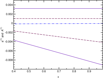
Figure 33: The leading recoil-order corrections to $a$ and $A$, $a^{(1)}$ and $A^{(1)}$, using $\lambda=1.2670$, $\tilde{g}_{2}=0$, $\tilde{f}_{2}=(\kappa_{p}-\kappa_{n})/2=1.8529$, and $\theta=0$. The solid (dashed) lines indicate the $Rx$ and $R$ terms in $a$ ($A$); the dashed-dot line indicates the $\epsilon/Rx$ term in $a$.

To test CVC in neutron decay, that is, to determine whether $\tilde{f}_{2}$ is given by the isovector magnetic moment remark , the coefficients multiplying $Rx$ must be determined; $f_{2}$ and $g_{2}$ can then be determined independently. A new method of measuring $a$ can determine its $x$ dependence, and a ${\cal O}(1\%)$ measurement is possible nista , whereas a new experiment to measure $A$ can potentially realize ${\cal O}(0.1\%)$ accuracy ucnA . A search for “new” physics implies that not only must the values of $\tilde{f}_{2}$ and $\tilde{g}_{2}$ be compared to SM expectations, but the structure of Eqs. (146,147) must also be tested. To realize this, it is crucial to determine $\tilde{f}_{2}$ and $\tilde{g}_{2}$ a plurality of ways, i.e., through different combinations of the $R$ and $Rx$ terms. Were $a$ and $A$ both measured to ${\cal O}(0.1)\%$, and $\tilde{f}_{2}$ and $\tilde{g}_{2}$ determined using the $E_{e}$-dependent terms, then $\delta\tilde{f}_{2}$ would be $2.5\%$ and $\delta\tilde{g}_{2}$ would be $0.26\lambda/2$ svgchi . Currently the most precise nuclear test of CVC/SCC is in the mass-12 system, in specific, through the measured difference of the $e^{\pm}$ angular distributions for purely aligned $1^{+}\to 0^{+}$ transitions, in ${}^{12}B(e^{-})$ and ${}^{12}N(e^{+})$ decay to ${}^{12}C$. This quantity is sensitive to both the weak magnetism and induced tensor terms in the nucleon weak current, though, unfortunately, the difference in the axial charge of the two mirror transitions, induced by isospin violation, enters as well. In the context of the impulse approximation, adopting the axial charge difference $\Delta y=0.10\pm 0.05$ computed in Ref. moritay , one finds $0.01\lambda\leq 2\tilde{g}_{2}\leq 0.34\lambda$, if CVC is assumed mina00 . The next generation of neutron decay experiments can test CVC/SCC with comparable accuracy and fewer assumptions than in the most precise nuclear test; CVC and SCC can also be tested independently.

As $\tilde{g}_{2}$ is of ${\cal O}(R)$ in the SM, the ability to extract $\tilde{f}_{2}$ and $\tilde{g}_{2}$ from the recoil corrections to $a$ and $A$, as per Eqs. (146,147), relies on the numerical magnitude of the next-to-leading order (NLO) recoil corrections morita75 ; holstein74 ; Zhang ; svgchi2 , i.e., on terms of ${\cal O}(R^{2},\epsilon)$. The uncertainties in these expressions are of particular interest. The ${\cal O}(\alpha)$ “outer” radiative corrections to $a$ and $A$ must also be applied, but are known sirshan . In NLO in recoil, the momentum transfer dependence of the form factors, as per $f_{i}(q^{2})=f_{i}[1+\xi_{i}{q^{2}}/{M^{2}_{n}}+...]$, as well as the induced pseudoscalar coupling constant $g_{3}$, enter for the first time. Only $f_{1}$ and $g_{1}$ appear in the allowed terms, so that only the $q^{2}$-dependences of these form factors are needed. However, the $q^{2}$-independent contributions which emerge from the recoil expansion of the terms in the hadronic matrix element and accompanying phase space dominate the NLO correction, and, in turn, the error in $g_{3}$ dominates the error in the NLO recoil correction. In our analysis we use the value of $g_{3}$ determined using heavy-baryon chiral perturbation theory (HBChPT) bernard1 . We conclude that the NLO recoil corrections, en masse, including an estimate of the correction to $\tilde{f}_{2}$ due to isospin violation, are sufficiently small that the LO recoil analysis can be used to bound $\tilde{g}_{2}$ until it is commensurate with its SM value Zhang ; svgchi2 .

65.2 Muon Capture

In this section we compare the theoretical result for $g_{3}$ we have employed bernard1 with the empirical value of $g_{3}$ determined in muon capture. Both ordinary muon capture (OMC), $\mu^{-}p\to\nu_{\mu}n$, and radiative muon capture (RMC), $\mu^{-}p\to\nu_{\mu}n\gamma$, on the proton permit the empirical determination of $g_{3}$. The kinematics of RMC can approach the $\pi$-pole more closely and as such is more sensitive to $g_{3}$. However, RMC yields a value of $g_{3}$ which is roughly 1.5 times larger than the HBChPT prediction, whereas the value determined in OMC is marginally consistent with theory gorringe . In specific, $g_{p}^{\rm th}=8.44\pm 0.23$ bernard1 , where $g_{P}=-m_{\mu}g_{3}(q^{2}=-0.88m_{\mu}^{2})/\hat{M}$ and $m_{\mu}$ is the muon mass, whereas an updated analysis gorringe of the TRIUMF RMC experiment wright yields $g_{p}^{\rm RMC}=12.4\pm 0.9\pm 0.4$. Extensive discussion of various resolutions exist in the literature, including molecular effects, (isospin-violating) electromagnetic effects, as well as criticisms of the computation of hadronic matrix elements, in particular of the inclusion of $\Delta$ degrees of freedom. No satisfactory explanation of the OMC and RMC data has been found to date bernard2 ; ando ; gorringe ; interestingly, the predicted photon energy spectrum in RMC determined in HBChPTrmc_hbchpt compares favorably with a reorganized chiral treatment in which the effects of the $\Delta$-resonance are included explicitly bernard2 .

66 Neutron Radiative $\beta$-Decay

We now turn to the discussion of the SM tests possible in neutron radiative $\beta$-decay. We consider two distinct tests: the determination of the weak transition form factor in $n\to pe^{-}\bar{\nu}_{e}\gamma$ to test the theoretical framework in which RMC is analyzed, as well as the determination of a “T-odd” correlation, sensitive to new sources of CP violation.

66.1 Weak Radiative Transition Form Factor

The photon in neutron radiative $\beta$-decay can be produced in bremsstrahlung from either charged particle in the final state, or it can be emitted from the effective weak vertex. The bremsstrahlung contributions form a portion of the “outer” radiative corrections in neutron $\beta$-decay sirshan , and the measurement of the photon energy spectrum in neutron radiative $\beta$-decay has been suggested as a means of testing a portion of those corrections gaponov . Rather, we believe the measurement of the photon energy spectrum offers a useful way of testing the theoretical frameworks used to analyze RMC, be it HBChPT rmc_hbchpt or reorganized HBChPT with an explicit $\Delta$ degree of freedom, for which the $N$ and $\Delta$ splitting is presumed small bernard2 . From this perspective, the bremsstrahlung photon emitted by the charged lepton is of lesser interest; rather the focus is on the $VV$ and $VA\,$ 4-point functions which must be calculated to determine the photon contribution from the hadronic side of the decay. In the static $W^{-}$ approximation, appropriate to the low-energy process we consider, the latter includes both bremsstrahlung from the proton as well as photon emission from the effective weak vertex. Nevertheless, the computed 4-point functions in concert with the leptonic bremsstrahlung contribution yields a prediction of the photon energy spectrum us ; its measurement is planned at NIST nistg .

66.2 “T-odd” Correlation

Radiative neutron $\beta$-decay admits the possibility of a pseudo-T-odd, P-odd correlation of the form $p_{p}\cdot(p_{e}\times p_{\gamma})$, as discussed in $K^{+}\to\pi^{0}e^{+}\nu_{e}\gamma$ decay braguta . Although such a contribution can be generated by electromagnetic final-state interactions in the SM, it also can be generated by new CP-violating phases in the first-generation, charged-current interaction gg , paralleling the discussion of the transverse muon polarization in $K^{+}\to\mu^{+}\nu_{\mu}\gamma$ decay specialK .

67 Summary

Precision, neutron-decay experiments are key to a rich array of low-energy, SM tests, providing useful constraints on the appearance of physics beyond the SM. We have considered the systematic determination of all of the couplings of the hadronic weak current and the SM tests such a determination entails, focusing on those tests alternative to the extraction of $V_{ud}$ and a test of the unitarity of the CKM matrix. We have considered how the determination of the coupling constants contained within the recoil corrections to the correlation coefficients $a$ and $A$ lead to independent tests of the CVC hypothesis as well as of the absence of SCC; such tests can be effected with fewer assumptions and with comparable precision to the most precise tests in nuclei. We have also considered how neutron radiative $\beta$-decay can be used to test the theoretical framework employed to extract the induced pseudoscalar coupling constant $g_{3}$ from RMC, as well as to search for new sources of CP violation.

*Radiative Corrections to the Neutron $\beta$-Decay Within the Standard Model and Their Role
for Precision Tests of the CKM-Unitarity Radiative Corrections to the Neutron $\beta$-Decay Within the Standard Model and Their Role for Precision Tests of the CKM-Unitarity G. G. Bunatian Email: bunat@cv.jinr.dubna.su

Nowadays, it has been well realized that careful, thorough and all-round study of the neutron $\beta-$decay conduces to gain an insight into the physical gist of semiweak processes and into the elementary particle physics in general d . In particular, the $CKM$ unitarity

$$|V_{ud}|^{2}+|V_{us}|^{2}+|V_{ub}|^{2}=1$$ (148)

is to be verified as strictly as possible ckm1 . That is why a grate deal of efforts has been directed past decade to measure, with a high accuracy, better than ${\sim}1\%$, the main characteristics of the $\beta-$decay of free neutrons: the lifetime $\tau$ t , the asymmetry factors (as a neutron is polarized) of the electron and antineutrino momentum distributions, $A$ a and $B$ ba respectively, the recoil proton distribution and the electron-antineutrino correlation coefficient $a$ p . Further experiments are believed to come to fruition before long.

In the report presented, the calculation of radiative corrections is based on the electroweak Lagrangian

$${\cal L}^{EW}(e,M_{Z},M_{W},m_{f},A_{\mu},W_{\mu}^{\pm},Z_{\mu},\psi_{f},\xi=1)$$ (149)

thoroughly elaborated in several review articles and books d ; ao ; h1 ; h2 ; b , and we pursue the methods expounded in these references. The electric charge $e=\sqrt{{\alpha}4{\pi}}$ and the masses of particles are chosen as the bare physical input parameters together with the physical fields $A_{\mu},W_{\mu}^{\pm},Z_{\mu},\psi_{f}$, the Feynman gauge, $\xi=1$, is presumed. This Lagrangian specifies the propagators of gauge boson, quark and lepton fields, $\;\;D^{A,W,Z}_{\mu\nu}(k^{2})\,,\,\;G_{f}(p)\,,\;$ and interactions between these fields

$${\cal L}^{EW}_{int}={\cal L}^{WWZ}+{\cal L}^{WWA}+{\cal L}^{Wff}+{\cal L}^{Zff}+{\cal L}^{Aff},$$ (150)

where $A,W,Z$ stand for electromagnetic, $W-$ and $Z-$boson fields, and $f$ renders various kinds of fermions. In further calculating the neutron $\beta-$decay amplitude in the one-loop approximation, we leave out the effect of Higgs-fermion interactions since they are of order $\sim{m_{f}}{/}{M_{W}}\ll 1$, the Higgs coupling to fermions ao ; h1 ; h2 ; b . The multiplicative renormalization is carried out, $g\rightarrow g{\cdot}z_{1}^{W,Z}{\cdot}(z_{2}^{W,Z})^{-3/2}\;,\;\;\Phi\rightarrow\Phi{\cdot}(z_{2}^{\Phi})^{1/2}\;,\;\;z=1+\delta{z}$ , accordingly the widely-applied on-mass-shell (OMS) renormalization scheme, $g$ and $\Phi$ represent generically couplings and fields ao ; h1 ; h2 ; b . The original Lagrangian (149) written in terms of the bare physical quantities is then decomposed into tree and counter terms as usually ao ; h1 ; h2 ; b

$${\cal L}^{EW}\Rightarrow{\cal L}_{tree}^{EW}(e,M_{W},M_{Z},m_{f},\Phi)$$

$$\hskip 31.29802pt+{\cal L}^{EW}_{ct}(e,M_{W},M_{Z},m_{f},\Phi,\delta M^{2}_{W},\delta M_{Z}^{2},\delta m^{2}_{f},\delta z_{1,2}^{\Phi}).$$ (151)

Upon renormalizing, not only the ultraviolet divergencies, occurring in the loop expansion, are absorbed into the infinite parts of the renormalization constants, but also the finite parts of radiative corrections are fixed. These lead to physically observable consequences.

The neutron $\beta$-decay

$$n\Longrightarrow p+e^{-}+\bar{\nu}+\gamma$$ (152)

can never be reduced to the pure quark decay $u\Rightarrow d+e^{-}+\bar{\nu}+\gamma$. As the nucleon is a complex composite system, strong quark-quark interactions must be properly taken into consideration. The total Lagrangian to describe (152) is the sum of electroweak and strong $qq-$interactions

$${\cal L}_{int}(x)={\cal L}^{EW}_{int}(x)+{\cal L}^{qq}_{str}(x),\;\;\;\;{\cal L}_{int}(x)\longrightarrow 0\;\;\;\text{when}\;\;\;x_{0}\longrightarrow\mp\infty$$ (153)

Without ${\cal L}^{qq}_{str}$, the nucleon wave function in quark variables reads as

$$\Phi^{q}_{N}(P_{N},\sigma_{N},x_{0})=\Phi^{q}_{0N}(P_{N},\sigma_{N})\equiv\Phi^{q}_{N}(P_{N},\sigma_{N},x_{0}{=}\pm\infty).$$ (154)

Here $P_{N},{\sigma}_{N}$ stand for momentum and spin variables of nucleons. The $S_{str}-$matrix, caused by ${\cal L}^{qq}_{str}$, transforms the wave function $\Phi^{q}_{0N}(P_{N},\sigma_{N})$ of the noninteracting quark system into the wave function of the physical nucleon $\Phi^{q}_{N}(P_{N},\sigma_{N},x_{0})$. So, with allowance for ${\cal L}_{str}^{qq}$ ,
$\Phi^{q}_{N}(P_{N},\sigma_{N},x_{0})={\cal S}_{str}(x_{0},\mp\infty)\Phi^{q}_{N}(P_{N},\sigma_{N},\mp\infty)={\cal S}_{str}(x_{0},\mp\infty)\Phi^{q}_{0N}(P_{N},\sigma_{N})\,,$ where

$${\cal S}_{str}(x_{0},-\infty)={\cal T}\exp\Bigl{(}i\int\limits_{-\infty}^{x_{0}}\mbox{d}x_{0}\int\mbox{d}{\bf x}{\cal L}^{qq}_{str}(x)\Bigr{)}\,,\;\;\;\;\;{\cal S}(t,t^{\prime})\cdot{\cal S}(t^{\prime},t_{0})={\cal S}(t,t_{0}).$$

$\cal T$ stands for the time-ordering operator.

The transition amplitude of (152) is given in the general form

$${\cal M}\cdot i(2\pi)^{4}\delta(P_{n}-P_{p}-p_{e}-p_{\gamma})=$$

$$\langle\Phi_{0p}^{q\,+}(P_{p},\sigma_{p}),\psi_{e}^{+}(p_{e}),A(p_{\gamma})|{\cal S}_{int}|\Phi_{0n}^{q}(P_{n},\sigma_{n}),\psi_{\nu}(-p_{\nu})\rangle\,,$$ (155)

with $S_{int}-$matrix dictated by (153)

$${\cal S}_{int}={\cal T}\exp\Bigl{(}i\int\mbox{d}^{4}x{\cal L}_{int}(x)\Bigr{)}={\cal T}\exp\Bigl{(}i\int\mbox{d}^{4}x[{\cal L}_{int}^{EW}(x)+{\cal L}_{str}^{qq}(x)]\Bigr{)}.$$ (156)

Nowadays, there sees no option but to parameterize the effect of strong interactions in treating the neutron $\beta-$decay.

At the lowest order in ${\cal L}^{EW}_{int}$, on the tree level, the amplitude of (152), with allowance for ${\cal L}_{str}^{qq}(x)$,

$${\cal M}^{0}=\bar{u}_{e}(p_{e})\Gamma_{\alpha}^{e\nu W}u_{\nu}(-p_{\nu})\cdot\bar{U}_{p}(P_{p})\Gamma_{N\,\beta}^{npW}U_{n}(P_{n})\cdot D_{\alpha\beta}^{W}(q)\,,$$ (157)

$${\Gamma}_{\alpha}^{e\nu W}={\Gamma}_{q\,\alpha}^{pnW}=\frac{e}{2\sqrt{2}s_{W}}\gamma_{\alpha}(1-\gamma^{5})\,,\;\;\;\;\Gamma_{N\,\alpha}^{npW}=|V_{ud}|\frac{e}{2\sqrt{2}s_{W}}{\cal J}_{np\;\alpha}(q)\,,$$

$$q=P_{n}-P_{p}-p_{e}-p_{\nu}\,\;\;\;\;q^{2}\ll M_{p}^{2}\ll M_{W}^{2}\,,\;\;\;\;D_{\alpha\beta}^{W}(q)=\frac{g_{\alpha\beta}}{q^{2}-M_{W}^{2}}=\frac{-g_{\alpha\beta}}{M^{2}_{W}}$$

is parameterized by introducing the nucleon weak transition current

$${\cal J}^{\beta}_{np}(k)=\gamma^{\beta}+g_{WM}\sigma^{\beta\nu}k_{\nu}-(\gamma^{\beta}g_{A}+g_{IP}k^{\beta})\gamma^{5}.$$ (158)

In (157), $u_{l}\,,\,\,U_{N}$ indicate Dirac spinors of leptons and nucleons, and the usual notations $c_{W}{=}{M_{W}}{/}{M_{Z}}\,,\,\,s_{W}^{2}=1-c_{W}^{2}$ are introduced. The Born amplitude (157) is written in terms of the non-renormalized vertices and $W-$propagator which will give place to the renormalized quantities $\hat{\Gamma}_{\alpha}^{e\nu W},\hat{\Gamma}_{N\,\beta}^{npW},\hat{D}_{\alpha\beta}^{W}$ in the one-loop calculation.

The evaluation of the renormalized pure lepton vertex with the counter terms obtained accordingly OMS gives

$$\Gamma_{\alpha}^{e\nu W}\Rightarrow$$

$$\hat{\Gamma}_{\alpha}^{e\nu W}=\Gamma^{e\nu W}_{\alpha}\Bigl{\{}1+\frac{\alpha}{4\pi}\Bigl{(}2\ln\frac{m}{\lambda}+\ln\frac{m}{M_{Z}}-\frac{9}{4}+\frac{3}{s^{2}_{W}}+\frac{6c_{W}^{2}-s_{W}^{2}}{s^{4}_{W}}\ln{c_{W}}\Bigr{)}\Bigr{\}}$$ (159)

As seen, this renormalized vertex in multiple of the nonrenormalized one. In evaluating (159) and hereafter, we neglect all the terms of the order $q{/}{M_{N,Z,S}}$, $m_{f}{/}{M_{N,Z,S}}$. All the masses are taken from pdg1 .

In the one-loop approximation, the renormalized $\hat{\Gamma}_{N\alpha}^{npW}-$vertex, which is due to the quark part of ${\cal L}_{int}^{EW}$, is defined by the matrix element which involves besides the electroweak interactions, ${\cal L}^{Zqq},{\cal L}^{Wqq},{\cal L}^{Aqq},{\cal L}^{ZWW},{\cal L}^{AWW}$, the strong $qq-$interaction ${\cal L}^{qq}_{str}$ as well, via ${\cal S}_{str}$. The processes of the different kinds contribute to $\hat{\Gamma}_{N\alpha}^{npW}$. In the piece of $\hat{\Gamma}_{N\alpha}^{npW}$ which involves the heavy virtual boson propagators $D^{W,Z}(k^{2})$ the integration over momenta $k$ in the loops involves, as a matter of fact, only the large values of momenta $k^{2}\sim M^{2}_{W,Z}$. Consequently, strong $qq-$interactions die out in intermediate states so that we deal with free quarks in the intermediate states in this case. In the part of $\hat{\Gamma}_{N\alpha}^{npW}$ involving a virtual photon, the photon propagator $D^{A}(k)$ is split into two pieces including large and small momenta

$$D^{A}_{\mu\nu}(x_{2}-x_{3})$$

$$=g_{\mu\nu}\int\frac{\mbox{d}^{4}k}{(2\pi)^{4}}\Bigl{(}\frac{1}{k^{2}-M^{2}_{S}+i0}+\frac{-M_{S}^{2}}{(k^{2}-\lambda^{2}+i0)(k^{2}-M^{2}_{S})}\Bigr{)}e^{-ik(x_{2}-x_{3})}$$ (160)

$$=D^{AS}_{\mu\nu}(x_{2}-x_{3})+D^{Al}_{\mu\nu}(x_{2}-x_{3}),$$

with the subsidiary matching parameter $M_{S}$ introduced thereby, $M_{p}^{2}\ll M^{2}_{S}\ll M_{W}^{2}$ sh . Quarks are free in the term involving $D^{AS}$, the “massive photon” propagator. The total renormalized vertex $\hat{\Gamma}_{N\,\alpha}^{npW}$ is written as

$$\hat{\Gamma}_{N\,\alpha}^{npW}=\hat{\Gamma}_{Ns\,\alpha}^{npW}+\hat{\Gamma}_{Nl\,\alpha}^{npW}.$$ (161)

The contribution $\hat{\Gamma}_{Ns\,\alpha}^{npW}$ from all the processes, where ${\cal L}^{qq}_{str}$ can be ignored in the intermediate states, proves to be

$$\hat{\Gamma}^{npW}_{Ns\,\alpha}(P_{n},P_{p},q)=\Gamma^{npW}_{N\,\alpha}\Biggl{\{}1+\frac{\alpha}{4\pi}\Bigl{(}\ln\frac{M_{S}}{M_{Z}}+\frac{3}{s^{2}_{W}}+\frac{6c^{2}_{W}-s^{2}_{W}}{s^{4}_{W}}\ln(c_{W})\Bigr{)}\Biggr{\}},$$ (162)

with the appropriate allowance for the counter terms obtained from ${\cal L}^{EW}_{int}$ , the “massive photon” propagator $D^{AS}$ replacing $D^{A}$.

As $\hat{\Gamma}^{npW}_{Nl\alpha}$ involves the “soft photon” propagator $D^{Al}(k^{2})$ , quarks in the intermediate state in $\hat{\Gamma}^{npW}_{Nl\alpha}$ posses small momenta and constitute baryonic states. Thus, $\hat{\Gamma}^{npW}_{Nl\alpha}$ in (161) incorporates the sum over the intermediate baryonic states, the bound states of strong interacting quarks. In the simplified case, when there are only pure unexcited nucleons in the intermediate states with the propagators $G_{N}(p_{N})$, and the nucleon formfactors are ignored, i.e. $f_{\alpha}^{p}=\gamma_{\alpha}\;,\;\;f^{n}_{\alpha}=0$, we arrive at

$$\hat{\Gamma}^{pnW}_{Nl\,\alpha}={\Gamma}^{npW}_{N\alpha}\biggl{(}\frac{1}{2}{\delta}{z_{0}^{p}}+\frac{1}{2}{\delta}{z_{0}^{n}}\biggr{)},$$ (163)

with the finite renormalization constants of the proton and neutron states

$${\delta}{z^{p}_{0}}=-\frac{\alpha}{4\pi}\Bigl{(}2\ln\frac{M_{S}}{M_{p}}+\frac{9}{2}-4\ln\frac{M_{p}}{\lambda}\Bigr{)}\,,\;\;\;\;{\delta}{z^{n}_{0}}=0.$$ (164)

To realize the accuracy of this result we have estimated the corrections to (163) due to the formfactors

$$f^{pp}_{\alpha}(k)=\Bigl{(}\gamma_{\alpha}+\frac{1.79}{2M_{p}}k^{\beta}{\sigma}_{\alpha\beta}\Bigr{)}\frac{-m^{2}_{\rho}}{k^{2}-m_{\rho}^{2}}\,,\;\;\;f^{nn}_{\alpha}=\Bigl{(}-\frac{1.93}{2M_{n}}\Bigr{)}\frac{-m^{2}_{\rho}}{k^{2}-m_{\rho}^{2}}\,,$$ (165)

where $m_{\rho}$ is the $\rho-$meson mass, and due to allowance for the $\Delta_{33}-$isobar in the intermediate states,

$$G_{N}(p)\longrightarrow G_{\Delta}(p)=\frac{\not p+M_{\Delta}}{p^{2}-M_{\Delta}^{2}+i0}.$$

These corrections prove to constitute no more than a few per cent to the quantity (163). The relations $M_{p,n}\ll M_{W,Z}\,,\;\;\;M^{2}_{p,n}\ll M^{2}_{S}\ll M^{2}_{W,Z}\,,\;\;\;m_{f}\ll M_{p,n}\,,\;\;\;q^{2}\ll M^{2}_{p,n}\,,\;\;\;M^{2}_{\Delta_{33}}-M^{2}_{p}\sim M^{2}_{p}$ are utilized through all the evaluations.

Thus, with the accuracy about a few per cent, the whole renormalized $Wnp-$vertex $\hat{\Gamma}^{npW}_{N\,\alpha}(P_{n},P_{p},q)=\hat{\Gamma}^{npW}_{Ns\,\alpha}(P_{n},P_{p},q)+\hat{\Gamma}^{npW}_{Nl\,\alpha}(P_{n},P_{p},q)$ is

$$\Gamma^{npW}_{N\,\alpha}\Biggl{\{}1+\frac{\alpha}{4\pi}\Bigl{(}\ln\frac{M_{p}}{M_{Z}}-2\ln\frac{\lambda}{M_{p}}-\frac{9}{4}+\frac{3}{s^{2}_{W}}+\frac{6c^{2}_{W}-s^{2}_{W}}{s^{4}_{W}}\ln(c_{W})\Bigr{)}\Biggr{\}}$$ (166)

is multiple of the nonrenormalized vertex $\Gamma_{N\alpha}^{npW}$.

Next, the propagator of virtual $W-$boson in ${\cal M}^{0}$ (157) modifies as

$$D^{W}(q)\Longrightarrow\hat{D}^{W}(q)=\frac{1}{q^{2}-M_{W}^{2}+\hat{\Sigma}^{W}(q^{2})}\approx\Bigl{(}-\frac{1}{M_{W}^{2}}\Bigr{)}\frac{1}{1-\frac{\hat{\Sigma}^{W}(0)}{M_{W}^{2}}}$$ (167)

which can be extracted from the $\mu-$decay analysis ms ; h2

$$\Bigl{(}\frac{e}{2\sqrt{2}s_{W}}\Bigr{)}^{2}\hat{D}^{W}(q)=-\frac{G_{\mu}(1-\delta_{\it v})}{\sqrt{2}}\ ,\;G_{\mu}=1.1663\cdot 10^{-5}\,\mbox{GeV}^{-2}\,,\;\delta_{\it v}\approx 0.006.$$

Then

$${\cal M}^{0}=-\frac{G\,|V_{ud}|}{\sqrt{2}}\bigl{(}\bar{u}_{e}(p_{e})\gamma_{\alpha}(1-\gamma_{5})u_{\nu}(-p_{\nu})\bigr{)}$$

$$\hskip 34.1433pt\cdot\bigl{(}\bar{U}_{p}(P_{p})\gamma^{\alpha}(1-\gamma_{5}g_{A})U_{n}(P_{n})\bigr{)}\,$$ (168)

$$\hskip 8.53581ptG=G_{\mu}(1-\delta_{\it v})$$

By now, we have considered the terms which stem from the Born amplitude ${\cal M}^{0}$ (157) by replacing the nonrenormalized vertices $\Gamma^{e\nu W}_{\alpha},\Gamma_{N\alpha}^{npW}$ and the $W-$boson propagator by renormalized ones. The total amplitude ${\cal M}$ of (152) also contains the part ${\cal M}_{2\gamma}$ which is of the second order in both lepton and quark electroweak interactions, usually referred to as a contribution from the “box diagrams”. The matrix element which defines ${\cal M}_{2\gamma}$ incorporates the terms of different nature. The term which is due to a photon exchange between quarks and leptons contains the photon propagator $D^{A}(k^{2})$ and is divided into two parts corresponding to large and small momenta transferred by the virtual photon, the “massive” $D^{AS}$ and “soft” $D^{Al}$ photon propagators respectively (160). The terms in ${\cal M}_{2\gamma}$ including heavy boson electroweak interactions with quarks and leptons, ${\cal L}^{Zqq},{\cal L}^{Wqq},{\cal L}^{Zee},{\cal L}^{Z\nu\nu},{\cal L}^{We\nu}$, are due to the $Z-$boson exchange between quarks and leptons. They contain the propagators $D^{W,Z}$ of virtual heavy gauge bosons. This case corresponds to large momenta, $\,q^{2}\sim M^{2}_{Z,W}\gg M_{p}^{2}$ , transferred from leptons to quarks. Strong $qq-$interactions in the intermediate states can be ignored in the terms containing the virtual heavy gauge bosons and “massive” photons. The contribution ${\cal M}_{2\gamma s}$ from these terms into the whole amplitude

$${\cal M}_{2\gamma}+{\cal M}_{2\gamma s}+{\cal M}_{2\gamma l}$$ (169)

is multiple of ${\cal M}_{0}$,

$${\cal M}_{2\gamma s}=-{\cal M}^{0}\frac{\alpha}{4\pi}\Biggl{\{}\Bigl{(}1+\frac{5c^{4}_{W}}{s^{4}_{W}}\Bigr{)}\ln{(c_{W})}-6\ln\frac{M_{W}}{M_{S}}\Biggr{\}}$$ (170)

The amplitude ${\cal M}_{2\gamma l}$ includes the “soft photon” propagator $D^{Al}$ which corresponds to small momenta $q^{2}<M^{2}_{S}$ transferred from leptons to quarks. Therefore the intermediate quark system posses small momenta so that we deal with an intermediate baryonic state $B$, a ground or excited nucleon state. Our calculation proves that leaving out all the excited states and presuming for the nucleon formfactors and nucleon transition current

$$f^{pp}_{\beta}=\gamma_{\beta}\,,\;\;\;f_{\beta}^{Bn}=0\,,\;\;\;{\cal J}_{\alpha}^{pn}=\gamma_{\alpha}(1-\gamma^{5}g_{A})$$ (171)

we commit no more than a few per cent error. With this accuracy

$${\cal M}_{2\gamma l}=\Bigl{(}\frac{e}{2\sqrt{2}s_{W}}\Bigr{)}^{2}|V_{ud}|\frac{1}{M_{W}^{2}}$$

$$\cdot\frac{\alpha}{4\pi}\Biggl{\{}\Biggl{(}\bar{u}_{e}(p_{e})\gamma^{\beta}(\not p_{e}+m)\gamma^{\alpha}(1-\gamma^{5})u_{\nu}(-p_{\nu})\frac{1}{2\varepsilon M_{p}v}$$

$$\times[\ln{(x)}\ln{\frac{\lambda}{m}}-\frac{1}{4}(\ln{(x)})^{2}+F(1/x-1)-{\pi^{2}v}{/}{\tilde{v}}]$$ (172)

$$-\bar{u}_{e}(p_{e})\gamma^{\beta}\gamma^{\delta}\gamma^{\alpha}(1-\gamma^{5})u_{\nu}(-p_{\nu})\frac{1}{2M_{p}}\big{[}-\frac{p_{\delta}}{v\varepsilon}\ln{(x)}+\delta_{0\delta}\bigl{(}\frac{1}{v}\ln{(x)}-2\ln{\frac{m}{M_{p}}})\bigr{]}\Biggr{)}$$

$$\times\bigl{(}\bar{U}_{p}(P_{p})\gamma_{\beta}(\not P_{p}+M_{p})\gamma_{\alpha}(1-\gamma^{5}g_{A})U_{n}(P_{n})\bigr{)}$$

$$-\bigl{(}\bar{u}_{e}(p_{e})\gamma^{\beta}\gamma^{\delta}\gamma^{\alpha}(1-\gamma^{5})u_{\nu}(-p_{\nu})\bigr{)}\bigl{(}\bar{U}_{p}(P_{p})\gamma_{\beta}\gamma^{\nu}\gamma_{\alpha}(1-g_{A}\gamma^{5})U_{n}(P_{n})\bigr{)}$$

$$\times g_{\delta\nu}\Bigl{(}\frac{3}{8}+\frac{1}{2}\bigl{(}\ln{\frac{M_{W}}{M_{p}}}-\frac{M_{W}^{2}}{M_{W}^{2}-M_{S}^{2}}\ln{\frac{M_{W}}{M_{S}}}\bigr{)}-\delta_{0\delta}\frac{1}{2}\Bigr{)}\Biggr{\}}$$

The electron energy $\varepsilon=\sqrt{m^{2}+p^{2}}\leq M_{n}-M_{p}\ll M_{p}$ . $F$ - Spens-function , ${\bf v}=\frac{\bf p}{\varepsilon}\,,$
$x={(1-v)}{/}{(1+v)}\;,\;\;\omega_{{\nu}0}=M_{n}-M_{p}-\varepsilon\,,$

$${\tilde{v}}({\varepsilon})=\frac{1}{2}\Biggl{(}\sqrt{(v+\frac{m\omega_{{\nu}0}}{M_{p}\varepsilon})^{2}+2v\frac{\omega_{{\nu}0}}{\varepsilon}(\frac{m}{M_{p}})^{2}}+\sqrt{(v-\frac{m\omega_{{\nu}0}}{M_{p}\varepsilon})^{2}-2v\frac{\omega_{{\nu}0}}{\varepsilon}(\frac{m}{M_{p}})^{2}}\,\,\Biggr{)}\,.$$

As seen, this part of the total transition amplitude ${\cal M}$ is not multiple of the Born amplitude ${\cal M}_{0}$ (157).

The amplitude of the real $\gamma-$radiation with momentum $\bf k$ and polarization $\mbox{{\boldmath$\epsilon$}}^{(r)}$

$${\cal M}^{(r)}_{1\gamma}(k)=\Bigl{(}\frac{e}{2\sqrt{2}s_{W}}\Bigr{)}^{2}|V_{ud}|\bigl{(}\frac{-1}{M_{W}^{2}}\Bigr{)}e\epsilon_{a}^{(r)}$$

$$\cdot\bigl{(}\bar{u}_{e}(p_{e})\gamma^{a}\frac{(\not p_{e}+\not k+m)}{(p_{e}+k)^{2}-m^{2}}\gamma^{\lambda}(1-\gamma^{5})u_{\nu}(-p_{\nu})\bigr{)}\times\bigl{(}\bar{U}_{p}(P_{p})\gamma_{\lambda}(1-g_{A}\gamma^{5})U_{n}(P_{n})\bigr{)}$$

$$(a,r=1,2,3)$$ (173)

is also not multiple of ${\cal M}^{0}$ (157).

Absolute square of the whole transition amplitude, up to the first $\alpha-$order,

$$|{\cal M}|^{2}=|{\cal M}^{R}+{\cal M}_{2\gamma l}+{\cal M}^{(r)}_{1\gamma}|^{2}\approx|{\cal M}^{R}|^{2}+|{\cal M}^{(r)}_{1\gamma}|^{2}+2\mbox{Re}[{\cal M}^{0}{\cal M}_{2\gamma l}],$$ (174)

where

$${\cal M}^{R}=\bigl{(}\bar{u}_{e}(p_{e})\hat{\Gamma}_{\alpha}^{e\nu\mu}u_{\nu}(-p_{\nu})\bigr{)}\times$$

$$\times\bigl{(}\bar{U}_{p}(P_{p})\hat{\Gamma}_{\beta}^{npW}U_{n}(P_{n})\bigr{)}D^{W}_{\alpha\beta}(p_{\nu}+p_{e})+{\cal M}_{2\gamma s}\approx$$

$$\approx{\cal M}^{0}\Bigl{\{}1-\frac{\alpha}{4\pi}\Bigr{(}2\ln{\frac{M_{Z}}{M_{p}}}+4\ln{\frac{\lambda}{m}}+\frac{9}{2}-\ln{\frac{M_{p}}{m}}-$$ (175)

$$-\frac{6}{s_{W}^{2}}-6\ln{\frac{M_{Z}}{M_{S}}}-\frac{3+4c^{2}_{W}}{s^{4}_{W}}\ln{(c_{W})}\Bigr{)}\Bigr{\}}$$

comprises all the terms proportional to the Born amplitude ${\cal M}^{0}$ (157). We calculate the $\beta-$decay probability of a polarized neutron (the polarization vector $\xi$) integrated over the final proton, antineutrino and photon momenta, and summarized over the polarizations of all the final particles

$$\mbox{d}{\bf W}(\varepsilon,{\bf p}_{e})=\mbox{d}{\bf W}^{R}(\varepsilon,{\bf p}_{e})+\mbox{d}{\bf W}_{1\gamma}(\varepsilon,{\bf p}_{e})+\mbox{d}{\bf W}_{2\gamma l}(\varepsilon,{\bf p}_{e})$$ (176)

where $\mbox{d}{\bf W}^{R},\;\mbox{d}{\bf W}_{1\gamma},\;\mbox{d}{\bf W}_{2\gamma l}$ come from $|{\cal M}^{R}|^{2},\;|{\cal M}^{(r)}_{1\gamma}|^{2},\;2\mbox{Re}[{\cal M}^{0}{\cal M}_{2\gamma l}]$ , respectively. $\;\;\mbox{d}{\bf W}^{R}(\varepsilon,{\bf p}_{e})$ is certainly proportional to the uncorrected, Born, decay probability

$$\mbox{d}{\bf W}^{0}(\varepsilon,{\bf p}_{e})=\frac{G^{2}}{2\pi^{3}}\varepsilon|{\bf p}_{e}|k_{m}^{2}\mbox{d}\varepsilon\frac{\mbox{d}{\bf n}}{4\pi}\bigl{(}1+3g_{A}^{2}+{\mbox{{\boldmath$v\xi$}}}2g_{A}(1-g_{A})\bigr{)}\,,$$ (177)

$${\bf n}={\bf p}_{e}{/}|{\bf p}_{e}|\,,\;\;\;{\mbox{{\boldmath$v$}}}={\bf p}_{e}{/}\varepsilon\,,\;\;\;k_{m}=M_{n}-M_{p}-\varepsilon,$$

whereas the contribution from the real $\gamma-$radiation and from the “box diagrams” containing nucleon in the intermediate state, $\mbox{d}{\bf W}_{1\gamma}(\varepsilon,{\bf p}_{e})$ and $\mbox{d}{\bf W}_{2\gamma l}(\varepsilon,{\bf p}_{e})$, are not multiple of $\mbox{d}{\bf W}^{0}(\varepsilon,{\bf p}_{e})$. Besides the terms proportional to $\mbox{d}{\bf W}^{0}(\varepsilon,{\bf p}_{e})$ they involve ones which are not.

Eventually, the electron momentum distribution in the $\beta-$decay of a polarized neutron is written as

$$\mbox{d}{\bf W}({\bf p}_{e},\varepsilon)=\frac{G^{2}}{2\pi^{3}}\varepsilon|{\bf p}_{e}|k_{m}^{2}\mbox{d}\varepsilon\frac{\mbox{d}{\bf n}}{4\pi}\bigl{\{}W_{0}(g_{A},\varepsilon)+\mbox{{\boldmath$v\xi$}}W_{\xi}(g_{A},\varepsilon)\bigr{\}}=$$

$$\mbox{d}{\bf W}^{0}({\bf p}_{e},\varepsilon)\cdot[{\cal B}(\varepsilon)+\tilde{C}_{1}(\varepsilon)]+\frac{G^{2}}{2\pi^{3}}\varepsilon|{\bf p}_{e}|k_{m}^{2}\mbox{d}\varepsilon\frac{\mbox{d}{\bf n}}{4\pi}\times$$

$$\Bigl{(}(1+3g_{A}^{2})\tilde{C}^{\prime}_{0}(\varepsilon)+2\mbox{{\boldmath$v\xi$}}g_{A}(1-g_{A})\tilde{C}^{\prime}_{\xi}(\varepsilon)+C_{0}(g_{A},\varepsilon)+C_{\xi}(g_{A},\varepsilon)\Bigr{)}.$$ (178)

$$W_{0}(g_{A},\varepsilon)=(1+3g_{A}^{2})[1+\tilde{C}_{0}(\varepsilon)+{\cal B}(\varepsilon)]+C_{0}(g_{A},\varepsilon),$$

$$W_{\xi}(g_{A},\varepsilon)=2g_{A}(1-g_{A})[1+\tilde{C}_{\xi}(\varepsilon)+{\cal B}(\varepsilon)]+C_{\xi}(g_{A},\varepsilon)$$

Here, all ${\cal B},{C}_{0},\tilde{C}_{0},{C}_{\xi},\tilde{C}_{\xi}$, are the cumbersome but rather plain functions of their arguments, directly obtained from Eqs. (159, 166, 167, 170, 172-176).

The relative modification of the total decay probability ,

$$\frac{\int\limits_{m}^{{\Delta}}\mbox{d}{\bf w}W_{0}({g_{A},\varepsilon})}{(1+3g_{A}^{2})\int\limits_{m}^{{\Delta}}\mbox{d}{\bf w}}-1=\delta W\,,$$ (179)

$$\Delta=M_{n}-M_{p}\,,\;\;\;\;\mbox{d}{\bf w}=\varepsilon|{\bf p}_{e}|k_{m}^{2}\mbox{d}\varepsilon\,\mbox{d}{\bf n},$$

amounts up to $\delta W\approx 8\%\,(\pm\lesssim 0.3\%)$. The uncorrected asymmetry factor of the electron angular distribution $A_{0}$ is replaced by corrected one $A({\varepsilon})$ accounting for the radiative corrections,

$$A_{0}=\frac{2g_{A}(1-g_{A})}{1+3g_{A}^{2}}\Longrightarrow\frac{W_{\xi}(g_{A},{\varepsilon})}{W_{0}({g_{A},\varepsilon})}=A({\varepsilon}).$$ (180)

The difference $\delta A=A(\varepsilon)-A_{0}\;$ amounts up to $\;\delta A\approx-1.9\%\,(\pm\lesssim 0.2\%)$. Practically, the same values of (179), (180) were acquired in the previous calculation i based immediately on the effective Lagrangian of the local $4$-fermion theory of weak interactions d . It is to emphasize ones again that the accuracy attainable in the presented calculation is about a few per cent to the obtained values of the radiative corrections, i.e. a few tenth of per cent, $\sim 0.01\%$, to the characteristics of the neutron $\beta-$decay, such as $W,A$. As was discussed above, the ambiguities come from the need to allow for strong $qq-$interactions and the nucleon compositeness, such as excited states and formfactors, associated with intrinsic structure. In particular, varying the parameter $M_{S}$ within the limits $3M_{p}<M_{S}<30M_{p}$ causes uncertainties $\sim 0.1\%$ in $\delta W,\delta A$. Introducing only the usual parameters $g_{A}\,,\,\,g_{WM}\,,\,\,g_{IP}$, describing the weak nucleon transition current, is not enough to parameterize the whole effect of strong interactions in treating the neutron $\beta-$decay.

Apparently, (178) can never be transformed to an expression multiple of (177), unlike the results asserted in several calculations sha ; gl1 ; gl2 ; gar which were entailed by Ref. sir where the total decay probability was reduced, to all intents and purposes, to the “model independent” part proportional merely to ${\cal M}^{0}$. That is why our results for quantities (179), (180) differ appreciably from the results asserted in Refs. sha ; gl1 ; gl2 ; gar ; sir : $\delta{W}_{MI}{\approx}5.4\%\,,\,\,\delta{A}_{MI}{\approx}0\%$. Because of the differences between these $\delta{W}_{MI}\,,\,\,\delta{A}_{MI}$ and our $\delta{W}\,,\,\,\delta{A}$, the $|V_{ud}|$ and $g_{A}$ values, ascertained from experimental data processing with allowance for $\delta{W}_{MI}\,,\,\,\delta{A}_{MI}$, would alter, when obtained with our $\delta{W}\,,\,\,\delta{A}$. The modifications are of the noticeable magnitude: $\delta g_{A}\approx 0.47\%\,,\,\,\delta|V_{ud}|{=}{-1.7\%}$. For instance, the values $g_{A}=1.2739\,,\,\,|V_{ud}|=0.9713$ given in a ; pdg1 will be modified to $g_{A}{\approx}1.28\,,\,\,|V_{ud}|{\approx}0.96$

So, the tenable calculation based on the electroweak theory provides the palpable results for radiative corrections which must be strictly allowed for in experimental data processing.

*Breaking of Isospin Symmetry in Nuclei
and Cabibbo-Kobayashi-Maskawa Unitarity Breaking of Isospin Symmetry in Nuclei
and Cabibbo-Kobayashi-Maskawa Unitarity H. Sagawa

68 Introduction

The isospin symmetry is the first dynamical symmetry in physics proposed by J. Heisenberg, 1932. This hypothesis relies entirely on the equivalence between the p-p and n-n two-body interactions. Experimentally, the validity of the isospin symmetry was proved by the finding of the isobaric analog state (IAS) in 1961 by J. D. Anderson and C. Wong. On the other hand, it is known that the two-body Coulomb interaction, the charge symmetry breaking (CSB) force and the charge independence breaking (CIB) force violate this symmetry and induce the impurity of isospin in the atomic nuclei. The question is how much the isospin impurity affects on important or not for the experimental determination of the vector coupling constant G_V of nucleon $\beta$ decay. Super-allowed Fermi $\beta$ decays have been studied intensively for several decades in relation to the vector coupling constant under the conserved vector current (CVC) hypothesis. Combining the vector coupling constant of nuclear $\beta$ decay with that of muon $\beta$ decay, it is possible to determine the mixing amplitude between ${\it u}$ and ${\it d}$ quarks in the first row of the Cabibbo-Kobayashi-Maskawa (CKM) unitary matrix. Thus, this amplitude , together with the mixing amplitudes of ${\it u}$ and ${\it s}$ quarks and ${\it u}$ and ${\it b}$ quarks, provides an opportunity to test experimentally the standard three-generation quark model for the electro-weak interaction.

Two nuclear medium corrections have been studied for obtaining the “ nucleus  independent ” ft valueOB89 ; THH77 . The first one is the “inner” radiative correction and the second one is the effect of isospin non-conserving forces in nuclei. These two corrections have been studied intensively during last two decades and found to be important to obtain the “nucleus independent” $ft$ value. However, there is still a substantial deviation from the unitarity in the empirical CKM matrix elements. It has been claimed that the empirical data of Fermi decay after subtracting the nuclear structure effects gives somewhat smaller value than that required by the unitary condition (3 times more than the standard deviation). In this studySGS96 , we will would like to pin down two new effects which have not been seriously discussed in the previous studies of the isospin mixings,i.e. , the isospin impurity of the core outside the shell model space and the effect of the charge symmetry breaking (CSB) and charge independence breaking (CIB) forces on the mean field potentials Wil93 ; SGS95 . It might be interesting to see how our model gives different results for the CKM unitarity problem since there are essential differences between our model and the previous studies. Particularly we study the Fermi $\beta$ decay in ¹⁰C, ¹⁴O, ²⁶Al, ³⁴Cl, ³⁸K, ⁴²Sc and ⁵⁴Co nuclei for which the most accurate experimental ${\it ft}$ values are available. We also report results of heavier nuclei ⁶²Ga, ⁶⁶As, and ⁷⁴Rb for further study of CVC hypothesis, and to clarify the differences between our model and previous calculations with different models.

69 RPA calculations for Fermi transitions

We have performed self-consistent Hartree-Fock(HF)+ random phase approximation (RPA) calculations. The CSB and CIB interactions are taken into account in the HF calculations. We take even-even nuclei (the daughter nuclei of the $\beta$ decay except for ¹⁰C and ¹⁴O) as the RPA vacuum and calculated the excited states with $J^{\pi}=0^{+}$ in odd-odd nuclei. The lowest states in the RPA spectra are identified as the IAS of the $\beta$ decay. We adopt the filling approximation for the RPA vacuum in which the particles occupy the HF single particle states from the bottom of the potential in order and the last orbit has a partially occupied configuration according to the mass number. The HF+RPA calculations are performed by using the harmonic oscillator basis. The model space adopted is 8 $\hbar\omega$ for ¹⁰C and ¹⁴O and 10 $\hbar\omega$ for other nuclei.

The quenching factor $\delta_{c}$ for the super-allowed transition is defined as

$$|\langle J^{\pi}=0^{+}T=1:\mbox{daughter}|T_{+}|J^{\pi}=0^{+}T=1:\mbox{mother}\rangle|^{2}\equiv 2(1-\delta_{c})$$ (181)

The results are shown in Fig. 34 with and without the CSB and CIB interactions. We pointed out that the sum rule values of the super-allowed Fermi transitions are enhanced substantially by the isospin impurity effect in nuclei with the mass $A\leq$20 SGS96 . Contrary to the results of the sum rule, the transitions are quenched substantially except for ¹⁰C. This is due to the fact that the isospin mixing of the mother state enhances the sum rule, but that of the daughter state cancels this enhancement in the transition. While there is no enhancement due to the couplings to the isovector giant monopole states, the coupling to neighboring $J^{\pi}$= 0⁺ states decrease the decay strength. This is the same mechanism as the finding of the previous shell model calculationsOB89 ; THH77 . The CSB and CIB interactions give 20-30 % larger quenching factors in all nuclei as shown in Fig. 34.

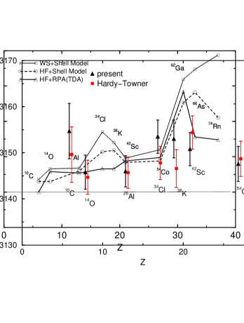
Figure 34: Calculated quenching factor $\delta_{c}$ of the super-allowed Fermi $\beta$ decay of seven $J$=0 odd-odd nuclei. The solid line with triangles is calculated by the HF and RPA (or TDA) with the Skyrme interaction SG2 + the CSB and CIB interactions. The results of HF(Woods-Saxon) + shell model denoted by the dashed(dotted) line with circles(squares) are taken from ref. OB95 .

70 CVC hypothesis and Cabibbo-Kobayashi-Maskawa (CKM) mixing matrix

Precise measurements of super-allowed $\beta$ decay between nuclei with ($J^{\pi}=0^{+},T=1)$ provide the most stringent probe of the electroweak interaction and has been the subject of intensive study for several decades. Since the axial current does not contribute to transitions in the lowest order, the experimental $ft$-value is directly related to the vector coupling constant $G_{V}$

$$ft=\frac{K}{G_{V}^{2}|M_{F}|^{2}}$$ (182)

where the constant $K/(\hbar c)^{6}$ and the matrix $M_{F}$ are defined as

$$K/(\hbar c)^{6} = 2\pi^{3}ln(2)\hbar/(m_{e}c^{2})^{6}$$

$$= (8120.271\pm 0.012)\times 10^{-10}GeV^{-4}\cdot s$$

$$|M_{F}|^{2} = |\langle J^{\pi}=0^{+}T=1:\mbox{daughter}$$ (184)

$$|T_{+}|J^{\pi}=0^{+}T=1:\mbox{mother}\rangle|^{2}$$ (185)

$$= 2(1-\delta_{c})$$

Up to now, nine $ft$ values of $0^{+}\rightarrow 0^{+}$transitions have been reported experimentally in enough accuracy of less than 0.2 % error to test the CVC hypothesis ; from the lightest ¹²C to the heaviest ⁵⁴Co. The constancy of these values is the key issue of the prediction of CVC hypothesis. Top of the CVC problem, the CKM mixing matrix between $u$ and $d$ quarks ($v_{ud}$) can be determined by comparing the decay rates for muon and nuclear Fermi $\beta$ decay. A test of the unitarity of the matrix , made possible by the empirical value $v_{ud}$, is an important measure of the accuracy for the three generation Standard model.

For these purposes, nucleus-dependent corrections should be subtracted from the experimental $ft$ values. The first is radiative corrections to the statistical rate function $f$, denoted conventionally $\delta_{R}$. There is also nucleus-independent radiative corrections $\Delta_{R}^{V}$. The factor $\delta_{R}$ is called the “inner” radiative correction and $\Delta_{R}^{V}$ is the “outer” radiative correction including axial-vector interference terms. The second correction is the nuclear structure factor due to the isospin impurity. Including all these corrections, the “nucleus-independent” $Ft$ value is defined as

$$Ft=ft(1+\delta_{R}+\Delta_{R}^{V})(1-\delta_{c})$$ (186)

and the matrix element $v_{ud}$ is given by

$$|v_{ud}|^{2}=\frac{\pi^{3}ln2}{Ft}\frac{\hbar^{7}}{G_{F}^{2}m_{e}^{5}c^{4}}=\frac{2984.38(6)}{Ft}$$ (187)

where the Fermi coupling $G_{F}$ is obtained from muon $\beta$ decay.

In table 1, we list the experimental $ft$ values, the nucleus dependent radiative correction $\delta_{R}$, the nuclear structure factor $\delta_{c}$ and the $Ft$ values. The outer radiative correction $\Delta_{R}^{V}$ is taken from ref. Tow95 ,

$$\Delta_{R}^{V}=(2.46\pm 0.09)\%$$ (188)

and added to obtain the $Ft$ values. The statistical factor $f$ adopted is slightly different from the values in ref.Wil93 , but does not make any significant change for the final results.

Figure 35: Nucleus independent $Ft$ values in eq. (24) of super-allowed Fermi transitions. The present results are plotted by black squares, while those of ref. Tow95 are given by black squares.

The average value $\bar{Ft}$ of 7 data in table 1 is

$$\bar{Ft}=3149.6\pm 1.5$$ (189)

The standard deviation $\sigma$ is 1.5 which could be small enough to justify the CVC hypothesis. There is no sigh of the Z-dependence of $Ft$ value in Fig. 4 which was claimed in ref.Wil93 to solve the deviation of the unitarity condition of the CKM matrix. In ref.Tow95 , the calculated $\bar{Ft}$ of the seven data is

$$\bar{Ft}=3148.2\pm 1.6\qquad,$$ (190)

while Ormand and Brown OB95 give

$$\bar{Ft}=3149.8\pm 1.8$$ (191)

The average value of our model is surprisingly close to the previous calculations in which the models are essentially different in the two points, i.e., the configuration space and the effect of CSB and CIB interactions in the mean field. The matrix element $v_{ud}$ is now calculated from eq. (27) to be

$$v_{ud}=0.9734(2)$$ (192)

The other two matrix elements $v_{us}$ and $v_{ub}$ are determined from independent experimental information of weak decays,

$$v_{us} = 0.2199(17)$$

$$v_{ub} < 0.0075(90\%\mbox{confidence level})$$ (193)

Finally, the sum of three matrix element becomes

$$|v_{ud}|^{2}+|v_{us}|^{2}+|v_{ub}|^{2}=0.9959(12)$$ (194)

which deviates (3-4) times more than the standard deviation $\sigma$= 0.0012 from the unitary condition. This deviation is certainly more than the ambiguity of nuclear structure effect since our RPA model prediction differs in only 0.05 % level from that of the shell model in average and corresponds to less than one standard deviation. It should be noticed that the final result in eq. (32) relies on many small effects of the radiative corrections and the nuclear structure. We calculated the $\delta_{c}$ and $Ft$ values by using another Skyrme interaction S3. The average $Ft$ value obtained is 3149.7 $\pm$1.5 which is essentially identical to that of SGII in table 1. However, the final conclusion will be easily changed by one unknown effect since the values discussed are always 1% level which will be certainly discarded in most of nuclear physics study.

Table 9: Empirical $ft$ values of super-allowed Fermi transitions and nucleus dependent corrections $\delta_{R}$ and $\delta_{c}$ The nucleus independent radiative corrections $\Delta_{R}^{V}$=2.46 $\pm$ 0.09 ( % ) are included in the $Ft$ values in eq. (24). The data of $ft,\delta_{R}$ and $\Delta_{R}^{V}$ are taken from ref. Tow95 .

SG2
A	$ft(s)$	$\delta_{R}$ (% )	$\delta_{c}(\%)$	$Ft(s)$
10C	3040.1 (50)	1.30 (4)	$-$0.01	3154.7 (60)
14O	3038.1 (18)	1.26 (5)	0.17	3145.8 (37)
26Al	3035.8 (17)	1.45 (2)	0.27	3146.0 (34)
34Cl	3048.4 (19)	1.33 (3)	0.33	3153.5 (36)
38K	3047.9 (26)	1.33 (4)	0.33	3153.0 (41)
42Sc	3045.1 (14)	1.47 (5)	0.44	3150.8 (36)
54Co	3045.8 (11)	1.39 (7)	0.49	3147.6 (38)
			ave.	3149.6 (15)

71 Summary

We studied the effect of isospin impurity on the super-allowed Fermi $\beta$-decay using the HF and RPA (or TDA) model. The Skyrme force SGII is adopted for both HF and RPA calculations. The CSB and CIB interactions are also taken into account in the HF calculations for the first time. The super-allowed Fermi transition probabilities of light nuclei ¹⁰C and ¹⁴O are shown to be quenched less than 0.2 % , while those of sd shell and pf-shell nuclei are quenched up to 1%. These calculated values are close to those obtained in the literatures with the HF and shell model calculations. It is interesting to notice that the shell model configuration space is 1 $\hbar\omega$ while, in our RPA calculations, we took into account up to 12 $\hbar\omega$ configuration in the harmonic oscillator basis. Another difference is the pairing which is properly taken into account in the shell model , but not in the HF + RPA calculations. We can notice in Fig. 2 that the quenching factor $\delta_{c}$ of the shell model is somewhat larger than those of our results in nuclei at the middle of the shells because of strong correlations in open-shell nuclei.

We estimate the so-called “nucleus independent” $Ft$ value taking into account both the nuclear structure and the radiation effects. The average $Ft$ value is obtained as

$${\bar{F}t}=3149.6(15)$$

which is very close to the ones reported by Chalk River group recently. It is shown that the values $Ft$ are rather Z-independent and no sign of the quadratic Z-dependence which is suggested by ref.Wil93 . Our result shows that the average $Ft$ value is still larger than the requested value to satisfy strictly the unitary condition of Cabibbo-Kobayashi-Maskawa matrix within 0.1 % level, although two new effects , the core polarization effects and the CSB and CIB interactions, are taken into account for the first time in our study.

*$g_{A}$ on the Lattice $g_{A}$ on the Lattice M. Göckeler, R. Horsley, D. Pleiter, P.E.L. Rakow, A. Schäfer,
G. Schierholz M. Göckeler, R. Horsley, D. Pleiter, P.E.L. Rakow, A. Schäfer,
G. Schierholz

72 What do we want to compute?

Lattice evaluations of $g_{A}$ make use of nucleon matrix elements of the axial vector current. For the quark flavors $q=u,d$ we have

$$\langle\mbox{proton},p,s|\bar{q}\gamma_{\mu}\gamma_{5}q|\mbox{proton},p,s\rangle=2\Delta q\cdot s_{\mu}\,,$$ (195)

where $p$ denotes the momentum of the proton and $s$ is its spin vector. In parton model language, $\Delta q$ is the fraction of the proton spin carried by the quarks of flavor $q$. Assuming perfect isospin symmetry we can write

$$\langle\mbox{proton},p,s|\bar{u}\gamma_{\mu}\gamma_{5}u-\bar{d}\gamma_{\mu}\gamma_{5}d|\mbox{proton},p,s\rangle$$

$$=\langle\mbox{proton},p,s|\bar{u}\gamma_{\mu}\gamma_{5}d|\mbox{neutron},p,s\rangle=2g_{A}\cdot s_{\mu}$$ (196)

and hence $g_{A}=\Delta u-\Delta d$.

73 What can we compute on the lattice?

The basic observables in lattice QCD are Euclidean $n$-point correlation functions. Since space-time has been discretised (with lattice spacing $a$) the path integral has become a high-dimensional integral over a discrete set of field variables. As the (Grassmann valued) quark fields appear bilinearly in the action, they can be integrated out analytically leaving behind the determinant of the lattice Dirac operator and products of quark propagators. The remaining integrals over the gluon fields can then be evaluated by Monte Carlo methods. In the quenched approximation, which will be employed throughout most of this paper, the determinant of the Dirac operator is replaced by 1. This approximation saves a lot of computer time, but it is hardly possible to estimate its accuracy.

Let us briefly sketch how hadronic matrix elements can be extracted from ratios of three-point functions over two-point functions. First, one has to choose suitable interpolating fields for the particle to be studied. For a proton with momentum $\vec{p}$ one may take

$$B_{\alpha}(t,\vec{p})=\sum_{x;x_{4}=t}\mathrm{e}^{-\mathrm{i}\vec{p}\cdot\vec{x}}\epsilon_{ijk}u^{i}_{\alpha}(x)u^{j}_{\beta}(x)(C\gamma_{5})_{\beta\gamma}d^{k}_{\gamma}(x)$$ (197)

and the corresponding $\bar{B}$, where $i$, $j$, …are color indices, $\alpha$, $\beta$, …are Dirac indices and $C$ is the charge conjugation matrix.

As the time extent $T$ of our lattice tends to $\infty$, the two-point correlation function becomes the vacuum expectation value of the corresponding Hilbert space operators with the Euclidean evolution operator ${\mathrm{e}}^{-Ht}$ in between, i.e. we have, omitting Dirac indices and momenta for simplicity:

$$\langle B(t)\bar{B}(0)\rangle\stackrel{{\scriptstyle T\to\infty}}{{=}}\langle 0|B{\mathrm{e}}^{-Ht}\bar{B}|0\rangle\,.$$ (198)

If in addition the time $t$ gets large, the ground state $|\mbox{proton}\rangle$ of the proton will dominate the sum over intermediate states between $B$ and $\bar{B}$, and the two-point function will decay exponentially with a decay rate given by the proton energy $E_{\mathrm{prot}}$:

$$\langle B(t)\bar{B}(0)\rangle\stackrel{{\scriptstyle T\to\infty}}{{=}}\langle 0|B{\mathrm{e}}^{-Ht}\bar{B}|0\rangle\stackrel{{\scriptstyle t\to\infty}}{{=}}\langle 0|B|\mbox{proton}\rangle{\mathrm{e}}^{-E_{\mathrm{prot}}t}\langle\mbox{proton}|\bar{B}|0\rangle+\cdots$$ (199)

Of course, if the momentum vanishes, we have $E_{\mathrm{prot}}=m_{\mathrm{prot}}$, the proton mass.

Similarly we have for a three-point function with the operator $\mathcal{O}$ whose matrix elements we want to calculate:

$$\langle B(t)\mathcal{O}(\tau)\bar{B}(0)\rangle$$

$$\stackrel{{\scriptstyle T\to\infty}}{{=}}\langle 0|B{\mathrm{e}}^{-H(t-\tau)}\mathcal{O}{\mathrm{e}}^{-H\tau}\bar{B}|0\rangle$$

$${}=\langle 0|B|\mbox{proton}\rangle{\mathrm{e}}^{-E_{\mathrm{prot}}(t-\tau)}\langle\mbox{proton}|\mathcal{O}|\mbox{proton}\rangle{\mathrm{e}}^{-E_{\mathrm{prot}}\tau}\langle\mbox{proton}|\bar{B}|0\rangle+\cdots$$

$${}=\langle 0|B|\mbox{proton}\rangle{\mathrm{e}}^{-E_{\mathrm{prot}}t}\langle\mbox{proton}|\bar{B}|0\rangle\langle\mbox{proton}|\mathcal{O}|\mbox{proton}\rangle+\cdots$$ (200)

if $t>\tau>0$. Hence the ratio

$$R\equiv\frac{\langle B(t)\mathcal{O}(\tau)\bar{B}(0)\rangle}{\langle B(t)\bar{B}(0)\rangle}=\langle\mbox{proton}|\mathcal{O}|\mbox{proton}\rangle+\cdots$$ (201)

will be independent of the times $\tau$ and $t$, if all time differences are so large that excited states can be neglected, and then $R$ yields the desired matrix element.

The proton three-point function for a two-quark operator contains quark-line connected as well as quark-line disconnected pieces. In the quark-line connected contributions the operator is inserted in one of the quark lines of the nucleon propagator, while in the disconnected pieces the operator is attached to an additional closed quark line which communicates with the valence quarks in the proton only via gluon exchange. In the limit of exact isospin invariance considered in this paper, the disconnected contributions of the $u$ quarks and the $d$ quarks cancel in the case of non-singlet two-quark operators. Fortunately, the operator needed for the evaluation of $g_{A}$ in Eq.(72) is of this type so that we do not have to cope with the disconnected contributions, which are very hard to compute.

74 Chiral symmetry

Chiral symmetry plays an important role in hadronic physics. Unfortunately, it is not straightforward to implement it on the lattice. “Traditional” formulations, like (improved) Wilson fermions break chiral symmetry explicitly at finite lattice spacing $a$. This has the consequence that the axial vector current has to be renormalized and chiral symmetry is only restored in the continuum limit $a\to 0$. However, the last years have seen a remarkable progress in this field. We have now “chirally symmetric” lattice formulations of the Dirac operator based on solutions of the Ginsparg-Wilson relation. These enjoy a lattice version of chiral symmetry even at finite lattice spacing such that physical consequences of chiral symmetry (e.g. Ward identities) hold already at finite $a$. In particular, there is an axial vector current which is not renormalized.

However, there is a price to be paid for these nice properties: Chirally symmetric lattice fermions need considerably more computer time than the “traditional” formulations. Therefore phenomenologically interesting results obtained with lattice fermions of this kind are only slowly beginning to appear.

A related problem is the chiral extrapolation: In the foreseeable future it will not be possible to perform simulations at the physical values of the masses of the $u$ and $d$ quarks. Hence results obtained at higher masses have to be extrapolated to the physical mass values. This extrapolation is, of course, the more reliable the smaller the masses in the simulation are. Since Ginsparg-Wilson fermions allow us to work with considerably lighter quarks than most other lattice fermions, their use will improve the quality of the results also in this respect.

75 Results

In Fig.36 taken from the review lat02 we show our own results (QCDSF and UKQCD collaborations) obtained with quenched and unquenched $O(a)$-improved Wilson fermions as well as results from the LHPC and SESAM collaborations LHPC who work with quenched and unquenched unimproved Wilson fermions. The $g_{A}$ values from the simulations have been extrapolated linearly in the quark mass to the chiral limit and are plotted versus $a^{2}$ in units of the “force scale” $r_{0}$ whose phenomenological value is $\approx 0.5\,\mbox{fm}$. Although the agreement between the various simulations is rather good (within the partially quite large statistical errors), the value obtained by a simple-minded continuum extrapolation is considerably smaller than the experimental value. Unquenching does not seem to have a big effect, which may be due to the rather large quark masses in the unquenched simulations.

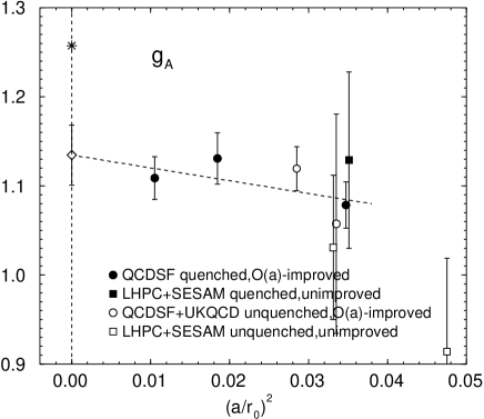
Figure 36: $g_{A}$ from quenched and unquenched simulations versus $a^{2}$ in units of $r_{0}\approx 0.5\,\mbox{fm}$. The experimental value is indicated by the asterisk.

Could the discrepancy between the simulations and experiment be caused by the chiral extrapolation? The data at finite masses which are behind the results displayed in Fig.36 do not show any deviation from linearity when plotted versus the quark mass. This is exemplified in Fig. 37 where the quenched QCDSF data with lattice artefacts subtracted are plotted versus the square of the pseudoscalar mass in units of $r_{0}^{-1}$. But will this linearity persist down to the physical mass? At small masses one has to worry about finite size effects, and simulations with unimproved Wilson fermions which we are performing show indeed some indications of such effects, but no significant deviation from linearity yet.

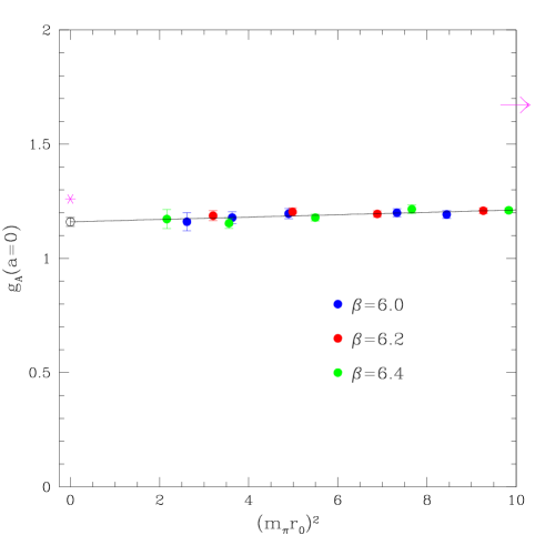
Figure 37: QCDSF results for $g_{A}$ from quenched improved Wilson fermions plotted versus the square of the pseudoscalar mass (proportional to the quark mass). The line shows a linear chiral extrapolation. The experimental value is indicated by the asterisk.

Clearer evidence for finite size effects in $g_{A}$ has been found by the RBC collaboration RBC in quenched simulations with domain wall fermions (an approximate realization of Ginsparg-Wilson fermions). For a more theoretical discussion of the volume dependence of $g_{A}$ we refer to the recent papers by Jaffe and Cohen jaffe . Hopefully, the influence of the finite volume will soon be better understood leading also to a clearer picture of the quark mass dependence. Recent results from chiral perturbation theory chpt shed more light on the problem of the chiral extrapolation. These developments should eventually enable us to increase the reliability of the lattice computations of $g_{A}$.

*CLEO-c and CESR-c: Allowing Quark Flavor Physics to Reach Its Full Potential CLEO-c and CESR-c: Allowing Quark Flavor Physics
to Reach Its Full Potential I. Shipsey

76 Executive Summary

The goals of quark flavor physics are: to test the consistency of the Standard Model (SM) description of quark mixing and CP violation, to search for evidence of new physics, and to sort between new physics scenarios initially uncovered at the LHC. This will require a range of measurements in the quark flavor changing sector of the SM at the per cent level. These measurements will come from a variety of experiments including BABAR and Belle and their upgrades, full exploitation of the facilities at Fermilab (CDF/D0/BTeV) and at the LHC (CMS/ATLAS/LHC-b), and experiments in rare kaon decays.

However, the window to new physics that quark flavor physics can provide, has a curtain drawn across it. The curtain represents hadronic uncertainty. The study of weak interaction phenomena, and the extraction of quark mixing matrix parameters remain limited by our capacity to deal with non-perturbative strong interaction dynamics. Techniques such as lattice QCD (LQCD) directly address strongly coupled theories and have the potential to eventually determine our progress in many areas of particle physics. Recent advances in LQCD have produced a wide variety of calculations of non-perturbative quantities with accuracies in the 10-20% level for systems involving one or two heavy quark such as $B$ and $D$ mesons, and $\Psi$ and $\Upsilon$ quarkonia. The techniques needed to reduce uncertainties to 1-2% precision exist, but the path to higher precision is hampered by the absence of accurate charm data against which to test and calibrate the new theoretical techniques.

To meet this challenge the CLEO collaboration has proposed to operate CLEO and CESR as a charm and QCD factory at charm threshold where the experimental conditions are optimal. In a three year focused program CLEO-c will obtain charm data samples one to two orders of magnitide larger than any previous experiment operating in this energy range, and with a detector that is significantly more powerful than any previous detector to operate at charm threshold. CLEO-c has the potential to provide a unique and crucial validation of LQCD with accuracies of 1-2%.

If LQCD is validated, CLEO-c data will lead to a dramatic improvement in our knowledge of the quark couplings in the charm sector. In addition CLEO-c validation of lattice calculations, combined with B factory, Tevatron, and LHC data will allow a significant improvement in our knowledge of quark couplings in the beauty sector. The impact CLEO-c will have on our knowledge of the CKM matrix makes the experiment an essential step in the quest to understand the origin of CP violation and quark mixing. CLEO-c allows quark flavor physics to reach its full potential, by enabling the heavy flavor community to draw back the curtain of hadronic uncertainty, and thereby see clearly through the window to the new physics that lies beyond the SM. Of equal importance, CLEO-c allows us to significantly advance our understanding and control over strongly-coupled, non-perturbatyive quantum field theories in general. An understanding of strongly coupled theories will be a crucial element in helping to interpret new phenomena at the high energy frontier.

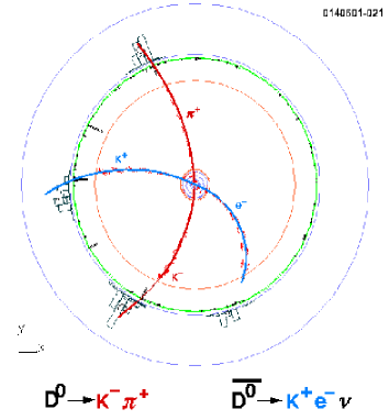
Figure 38: A doubly tagged event at the $\psi(3770)$.

77 Introduction

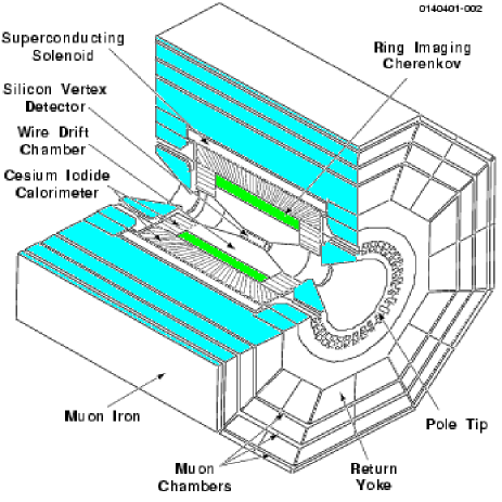
Figure 39: The CLEO III detector.

For many years, the CLEO experiment at the Cornell Electron Storage Ring, CESR, operating on the $\Upsilon$(4S) resonance, has provided most of the world’s information about the $B_{d}$ and $B_{u}$ mesons. At the same time, CLEO, using the copious continuum pair production at the $\Upsilon$(4S) resonance has been a leader in the study of charm and $\tau$ physics. Now that the asymmetric B factories have achieved high luminosity, CLEO is uniquely positioned to advance the knowledge of quark flavor physics by carrying out several measurements near charm threshold, at center of mass energies in the 3.5-5.0 GeV region. These measurements address crucial topics which benefit from the high luminosity and experimental constraints which exist near threshold but have not been carried out at existing charm factories because the luminosity has been too low, or have been carried out previously with meager statistics. They include:

1. Charm Decay constants $f_{D},f_{D_{s}}$

2. Charm Absolute Branching Fractions

3. Semileptonic decay form factors

4. Direct determination of $V_{cd}$ & $V_{cs}$

5. QCD studies including:
   Charmonium and bottomonium spectroscopy
   Glueball and exotic searches
   Measurement of R between 3 and 5 GeV, via scans
   Measurement of R between 1 and 3 GeV, via ISR

6. Search for new physics via charm mixing, CP violation and rare decays

7. $\tau$ decay physics

The CLEO detector can carry out this program with only minimal modifications. The CLEO-c project is described at length in cleo-c - maravin . A very modest upgrade to the storage ring is required to achieve the required luminosity. Below, we summarize the advantages of running at charm threshold, the minor modifications required to optimize the detector, examples of key analyses, a description of the proposed run plan, and a summary of the physics impact of the program.

Table 10: Summary of CLEO-c charm decay measurements.

Topic	Reaction	Energy	$L$	current	CLEO-c
		(MeV)	$(fb^{-1})$	sensitivity	sensitivity
Decay constant
$f_{D}$	$D^{+}\to\mu^{+}\nu$	3770	3	UL	2.3%
$f_{D_{s}}$	$D_{s}^{+}\to\mu^{+}\nu$	4140	3	14%	1.9%
$f_{D_{s}}$	$D_{s}^{+}\to\mu^{+}\nu$	4140	3	33%	1.6%
Absolute Branching Fractions
$Br(D^{0}\to K\pi)$		3770	3	2.4%	0.6%
$Br(D^{+}\to K\pi\pi)$		3770	3	7.2%	0.7%
$Br(D_{s}^{+}\to\phi\pi)$		4140	3	25%	1.9%
$Br(\Lambda_{c}\to pK\pi)$		4600	1	26%	4%

77.1 Advantages of running at charm threshold

The B factories, running at the $\Upsilon$(4S) will have produced 500 million charm pairs by 2005. However, there are significant advantages of running at charm threshold:

1. Charm events produced at threshold are extremely clean.

2. Double tag events, which are key to making absolute branching fraction measurements, are pristine.

3. Signal/Background is optimum at threshold.

4. Neutrino reconstruction is clean.

5. Quantum coherence aids $D$ mixing and CP violation studies.

These advantages are dramatically illustrated in Fig. 1, which shows a picture of a simulated and fully reconstructed $\psi(3770)\to D\bar{D}$ event.

77.2 The CLEO-III Detector : Performance, Modifications and issues

The CLEO III detector, shown in Figure 39, consists of a new silicon tracker, a new drift chamber, and a Ring Imaging Cherenkov Counter (RICH), together with the CLEO II/II.V magnet, electromagnetic calorimeter and muon chambers. The upgraded detector was installed and commissioned during the Fall of 1999 and Spring of 2000. Subsequently operation has been very reliable (see below for a caveat) and a very high quality data set has been obtained. To give an idea of the power of the CLEO III detector in Figure 40 (left plot) the beam constrained mass for the Cabibbo allowed decay $B\to D\pi$ and the Cabibbo suppressed decay $B\to DK$ with and without RICH information is shown.

The latter decay was extremely difficult to observe in CLEO II/II.V which did not have a RICH detector. In the right plot of Figure 40 the penguin dominated decay $B\to K\pi$ is shown. This, and other rare $B$ decay modes are observed in CLEO III with branching ratios consistent with those found in CLEO II/II.V, and are also in agreement with recent Belle and BABAR results. Figure 40 is a demonstration that CLEO III performs very well indeed.

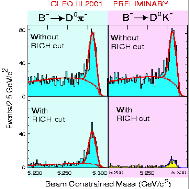
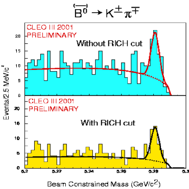
Figure 40: (Top) Beam constrained mass for the Cabibbo allowed decay $B\to D\pi$ and the Cabibbo suppressed decay $B\to DK$ with and without RICH information. The latter decay was extremely difficult to observe in CLEO II/II.V which did not have a RICH detector. (Bottom) The penguin dominated decay $B\to K\pi$. Both of these modes are observed in CLEO III with branching ratios consistent with those found in CLEO II/II.V.

Unfortunately, there is one detector subsystem that is not performing well. The CLEO III silicon has experienced an unexpected and unexplained loss of efficiency. The silicon detector will be replaced with a wire vertex chamber for CLEO-c. We note that if one was to design a charm factory detector from scratch the tracking would be entirely gas based to ensure that the detector material was kept to a minimum. CLEO-c simulations indicate that a simple six layer stereo tracker inserted into the CLEO III drift chamber, as a silicon detector replacement, would provide a system with superior momentum resolution compared to the current CLEO III tracking system.

Due to machine issues we plan to lower the solenoid field strength to 1.0 T from 1.5 T. All other parts of the detector do not require modification. The dE/dx and Ring Imaging Cerenkov counters are expected to work well over the CLEO-c momentum range. The electromagnetic calorimeter works well and has fewer photons to deal with at 3-5 GeV than at 10 GeV. Triggers will work as before. Minor upgrades may be required of the Data Acquisition system to handle peak data transfer rates. The conclusion is that, with the addition of the replacement wire chamber, CLEO is expected to work well in the 3-5 GeV energy range at the expected rates.

77.3 Machine Conversion

Electron positron colliders are designed to operate optimally within a relatively narrow energy range. As the energy is reduced below design, there is a significant reduction in synchrotron radiation, which is the primary means of cooling the beam. In consequence, the luminosity drops, roughly as the beam energy to the fourth power. Without modification to the machine, CESR performance in the 3-5 GeV energy range would be modest, well below $10^{31}{\rm cm}^{-2}{\rm s}^{-1}$. CESR conversion to CESR-c requires 18 m of wiggler magnets, to increase transverse cooling, at a cost of $\sim$ $4M. With the wigglers installed, CESR-c is expected to achieve a luminosity in the range $2-4\times 10^{32}{\rm cm}^{-2}{\rm s}^{-1}$ where the lower (higher) luminosity corresponds to $\sqrt{s}=3.1(4.1){\rm GeV}$.

77.4 Examples of analyses with CLEO-c

The main targets for the CKM physics program at CLEO-c are absolute branching ratio measurements of hadronic, leptonic and semileptonic decays. The first of these provides an absolute scale for all charm and hence all beauty decays. The second measures decay constants and the third measures form factors and, in combination with theory, allows the determination of $V_{cd}$ and $V_{cs}$.

Absolute branching ratios

The key idea is to reconstruct a $D$ meson in any hadronic mode. This, then, constitutes the tag. Figure 41 shows tags in the mode $D\to K\pi$. Note the y axis is a log scale. Tag modes are very clean. The signal to background ratio is $\sim$ 5000/1 for the example shown. Since $\psi(3770)\to D\bar{D}$, reconstruction of a second D meson in a tagged event to a final state X, corrected by the efficiency which is very well known, and divided by the number of D tags, also very well known, is a measure of the absolute branching ratio $Br(D\to X)$. Figure 42 shows the $K^{-}\pi^{+}\pi^{+}$ signal from doubly tagged events. It is approximately background free. The simplicity of $\psi(3770)\to D\bar{D}$ events combined with the absence of background allows the determination of absolute branching ratios with extremely small systematic errors. This is a key advantage of running at threshold.

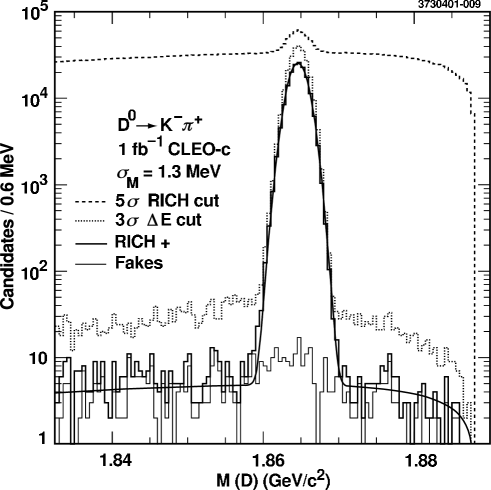
Figure 41: $K\pi$ invariant mass in $\psi(3770)\to D\bar{D}$ events showing a strikingly clean signal for $D\to K\pi$. The y axis is a logarithmic scale. The signal to background ratio is $\sim$ 5000/1.

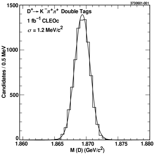
Figure 42: $K\pi\pi$ invariant mass in $\psi(3770)\to D\bar{D}$ events where the other D in the event has already been reconstructed. A clean signal for $D\to K\pi\pi$ is observed and the absolute branching ratio $Br(D\to K\pi\pi)$ is measured by counting events in the peak.

Leptonic decay $D_{s}\to\mu\nu$

This is a crucial measurement because it provides information which can be used to extract the weak decay constant, $f_{D_{s}}$. The constraints provided by running at threshold are critical to extracting the signal.

The analysis procedure is as follows:

1. Fully reconstruct one $D_{s}$, this is the tag.

2. Require one additional charged track and no additional photons.

3. Compute the missing mass squared ($m_{\nu}^{2}$) which peaks at zero for a decay where only a neutrino is unobserved.

The missing mass resolution, which is of order $\sim m_{\pi^{0}}$, is sufficient to reject the backgrounds to this process as shown in Fig. 43. There is no need to identify muons, which helps reduce the systematic error. One can inspect the single prong to make sure it is not an electron. This provides a check of the background level since the leptonic decay to an electron is severely helicity-suppressed and no signal is expected in this mode.

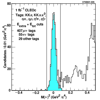
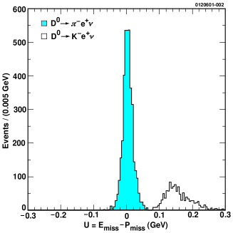
Figure 43: (Left) Missing mass squared for $D_{s}\bar{D_{s}}$ tagged pairs produced at $\sqrt{s}=4100$ MeV. Events due to the decay $D_{s}\to\mu\nu$ are shaded. (Right) The difference between the missing energy and missing momentum in $\psi(3770)\to D\bar{D}$ tagged events for the Cabibbo suppressed decay $D\to\pi\ell\nu$ (shaded). The unshaded histogram arises from the ten times more copiously produced Cabibbo allowed transition $D\to K\ell\nu$ where the $K$ is outside the fiducial volume of the RICH.

Semileptonic decay $D\to\pi e^{+}\nu$

The analysis procedure is as follows:

1. Fully reconstruct one D, this constitutes the tag.

2. Identify one electron and one hadronic track.

3. Calculate the variable, $U=E_{miss}-P_{miss}$, which peaks at zero when only a neutrino has escaped detection, which is the case for semileptonic decays.

Using the above procedure results in the right plot of Figure 43. With CLEO-c for the first time it will become possible to make precise branching ratio and absolute form factor measurements of every charm meson semileptonic pseudoscalar to pseudoscalar and pseudoscalar to vector transition. This will be a lattice validation data set without equal. Figure 44 shows the current precision with which the absolute semileptonic branching ratios of charm particles are known, and the precision attainable with CLEO-c.

77.5 Run Plan

CLEO-c must run at various center of mass energies to achieve its physics goals. The “run plan” currently used to calculate the physics reach is given below. This plan assumes CESR-c achieves design luminosity. Item 1 is prior to machine conversion, while the remaining items are post machine conversion.

1. 2002 : $\Upsilon$’s – 1-2 $fb^{-1}$ each at $\Upsilon(1S),\Upsilon(2S),\Upsilon(3S)$
   Spectroscopy, electromagnetic transition matrix elements, the leptonic width. $\Gamma_{ee}$, and searches for the yet to be discovered $h_{b},\eta_{b}$ with 10-20 times the existing world’s data sample. As of July 2002, most of this data has been collected.

2. 2003 : $\psi(3770)$ – 3 $fb^{-1}$
   30 million events, 6 million tagged D decays (310 times MARK III)

3. 2004 : 4100 MeV – 3 $fb^{-1}$
   1.5 million $D_{s}D_{s}$ events, 0.3 million tagged $D_{s}$ decays (480 times MARK III, 130 times BES)

4. 2005 : $J/\psi$ – 1 $fb^{-1}$
   1 billion $J/\psi$ decays (170 times MARK III, 20 times BES II)

77.6 Physics Reach of CLEO-c

Tables 10, 11 , and 12, and Figures 44 and 45 summarize the CLEO-c measurements of charm weak decays, and compare the precision obtainable with CLEO-c to the expected precision at BABAR which expects to have recorded about 500 million charm pairs by 2005. While BABAR data allows improvement in the precision with which these quantities can be measured, CLEO-c clearly achieves far greater precision for many measurements. The reason for this is the ability to measure absolute branching ratios by tagging, and the absence of background at threshold. For charm quantities where CLEO-c is not dominant, it will remain comparable in sensitivity, and complementary in technique, to the B factories. Also shown in Table 12 is a summary of the data set size for CLEO-c and BES II at the $J/\psi$ and $\psi^{\prime}$, and the precision with which R, the ratio of the $e^{+}e^{-}$ annihilation cross section into hadrons to mu pairs, can be measured. The CLEO-c data sets are over an order of magnitude larger, the precision with which R is measured is a factor of three higher, in addition the CLEO detector is vastly superior to the BES II detector.

Taken together the CLEO-c datasets at the $J/\psi$ and $\psi^{\prime}$ will be qualitatively and quantitatively superior to any previous dataset in the charmonium sector thereby providing discovery potential for glueballs and exotics without equal.

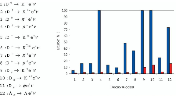
Figure 44: Absolute branching ratio current precision from the PDG (left entry) and precision attainable at CLEO-c (right entry ) for twelve semileptonic charm decays.

Table 11: Summary of direct CKM reach with CLEO-c

Topic	Reaction	Energy	$L$	current	CLEO-c
		(MeV)	$(fb^{-1})$	sensitivity	sensitivity
$V_{cs}$	$D^{0}\to K\ell^{+}\nu$	3770	3	16%	1.6%
$V_{cd}$	$D^{0}\to\pi\ell^{+}\nu$	3770	3	7%	1.7%

Table 12: Comparision of CLEO-c reach to BABAR and BES

Quantity	CLEO-c	BaBar	Quantity	CLEO-c	BES-II
$f_{D}$	2.3%	10-20%	#$J/\psi$	$10^{9}$	$5\times 10^{7}$
$f_{D_{s}}$	1.7%	5-10%	$\psi^{\prime}$	$10^{8}$	$3.9\times 10^{6}$
$Br(D^{0}\to K\pi)$	0.7%	2-3%	4.14 GeV	$1fb^{-1}$	$23pb^{-1}$
$Br(D^{+}\to K\pi\pi)$	1.9%	3-5%	3-5 R Scan	2%	6.6%
$Br(D_{s}^{+}\to\phi\pi)$	1.3%	5-10%

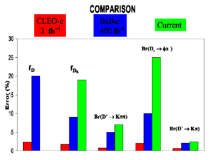
Figure 45: Comparison of CLEO-c (left) BABAR (center) and PDG2001 (right) for the charm meson decay constants and three important charm meson hadronic decay branching ratios.

77.7 CLEO-c Physics Impact

CLEO-c will provide crucial validation of Lattice QCD, which will be able to calculate with accuracies of 1-2%. The CLEO-c decay constant and semileptonic data will provide a “golden”, and timely test while CLEO-c QCD and charmonium data provide additional benchmarks. CLEO-c will provide dramatically improved knowledge of absolute charm branching fractions which are now contributing significant errors to measurements involving b’s in a timely fashion. CLEO-c will significantly improve knowledge of CKM matrix elements which are now not very well known. $V_{cd}$ and $V_{cs}$ will be determined directly by CLEO-c data and LQCD, or other theoretical techniques. $V_{cb},V_{ub},V_{td}$ and $V_{ts}$ will be determined with enormously improved precision using B factory and Tevatron data, once the CLEO-c program of lattice validation is complete. Table 13 provides a summary of the situation. CLEO-c data alone will also allow new tests of the unitarity of the CKM matrix. The unitarity of the second row of the CKM matrix will be probed at the 3% level. Of particular relevance to this workshop CLEO-c will make a measurement of $V_{cd}$ to better than 2% precision. This measurement can be combined with the beautiful measurements of $V_{ud}$ discussed elsewhere in these proceedings to test of the unitarity of the first column of the CKM matrix to a precision similar to that with which the first row is now known. CLEO-c data will also test unitarity by measuring the ratio of the long sides of the squashed $cu$ triangle to 1.3%.

Finally the potential to observe new forms of matter; glueballs, hybrids, etc. in $J/\psi$ decays and new physics through sensitivity to charm mixing, CP violation, and rare decays provides a discovery component to the program.

Table 13: Current knowledge of CKM matrix elements (row one). Knowledge of CKM matrix elements after CLEO-c (row two). The improvement in the precision with which $V_{cd}$ and $V_{cs}$ are known is attainable with CLEO-c data combined with Lattice QCD. The improvement in precision with which $V_{cb}$, $V_{ub}$, $V_{td}$, and $V_{ts}$ are known is obtained from CLEO-c validated Lattice QCD calculations and B factory and Tevatron data.

$V_{cd}$	$V_{cs}$	$V_{cb}$	$V_{ub}$	$V_{td}$	$V_{ts}$
7%	16%	5%	25%	36%	39%
1.7%	1.6%	3%	5%	5%	5%

I would like to thank my CLEO colleagues for providing the opportunity to represent the collaboration at this conference. It is a privilege to be part of the CLEO collaboration. I thank Ikaros Bigi, Gustavo Burdman, Andreas Kronfeld, Peter Lepage, Zoltan Ligeti and Matthias Neubert for valuable discussions. Finally, I thank Hans Abele and his support team for the superb organization of this conference.

*Perspectives on Measuring $V_{us}$ at KLOE Perspectives on Measuring $V_{us}$ at KLOE The KLOE Collaboration A. Aloisio, F. Ambrosino, A. Antonelli, M. Antonelli, C. Bacci, G. Bencivenni, S. Bertolucci, C. Bini, C. Bloise, V. Bocci, F. Bossi, P. Branchini, S. A. Bulychjov, R. Caloi, P. Campana, G. Capon, G. Carboni, M. Casarsa, V. Casavola, G. Cataldi, F. Ceradini, F. Cervelli, F. Cevenini, G. Chiefari, P. Ciambrone, S. Conetti, E. De Lucia, P. De Simone, G. De Zorzi, S. Dell’Agnello, A. Denig, A. Di Domenico, C. Di Donato, S. Di Falco, B. Di Micco, A. Doria, M. Dreucci, O. Erriquez, A. Farilla, G. Felici, A. Ferrari, M. L. Ferrer, G. Finocchiaro, C. Forti, A. Franceschi, P. Franzini, C. Gatti, P. Gauzzi, S. Giovannella, E. Gorini, E. Graziani, S. W. Han, M. Incagli, W. Kluge, V. Kulikov, F. Lacava, G. Lanfranchi, J. Lee-Franzini, D. Leone, F. Lu, M. Martemianov, M. Matsyuk, W. Mei, L. Merola, R. Messi, S. Miscetti, M. Moulson, S. Müller, F. Murtas, M. Napolitano, A. Nedosekin, F. Nguyen, M. Palutan, E. Pasqualucci, L. Passalacqua, A. Passeri, V. Patera, E. Petrolo, L. Pontecorvo, M. Primavera, F. Ruggieri, P. Santangelo, E. Santovetti, G. Saracino, R. D. Schamberger, B. Sciascia, A. Sciubba, F. Scuri, I. Sfiligoi, A. Sibidanov, T. Spadaro, E. Spiriti, G. L. Tong, L. Tortora, P. Valente, B. Valeriani, G. Venanzoni, S. Veneziano, A. Ventura, S. Ventura, R. Versacci, G. W. Yu. presented by E. De Lucia

The KLOE experiment at DA$\Phi$NE

The KLOEkp detector at DA$\Phi$NE dafne , the Frascati $\phi$-factory, started data taking in April 1999. The DA$\Phi$NE  e⁺-e^- collider operates at the center of mass of the $\phi$(1020) meson producing almost monochromatic K${}^{0}_{S}$ and K${}^{0}_{L}$ pairs, K⁺ and K^-  pairs and all other $\phi$ decay products. Moreover at DA$\Phi$NE   kaons are produced with a $\sim 110-125$ MeV/c momentum and their decay lengths are $\lambda_{S}\sim 0.6$ cm, $\lambda_{L}\sim 340$ cm and $\lambda_{\pm}\sim 90$ cm. The unique feature of a $\phi$-factory is the tagging: the detection of a long-lived neutral kaon guarantees the presence of a K${}^{0}_{S}$ of given momentum and direction and viceversa, the same holds for charged kaons.

During 2002 data taking DA$\Phi$NE   reached a peak luminosity of $\simeq 8\times 10^{31}$cm^-2s^-1 .

The integrated luminosity is $\sim 500~{}pb^{-1}$ for a total number of $1.5\times 10^{6}~{}~{}K^{+}K^{-}$ pairs per $pb^{-1}$ and $10^{6}~{}~{}K_{L}K_{S}$ pairs per $pb^{-1}$.

The KLOE detectorkp ; tp consists of a large cylindrical drift chamber surrounded by a hermetic electromagnetic calorimeter. A superconducting coil and an iron yoke surrounding the whole detector provide a 0.52 T magnetic field.

The drift chamberdpap (DC) with 4 m diameter and 3.3 m length, has a total number of 52140 wires, arranged in 12582 cells distributed over 58 concentric layers and with an all-stereo geometry. In order to maximize transparency to photons and reduce K${}^{0}_{L}$ regeneration, the mechanical support of the drift chamber is made of carbon fiber-epoxy composite and the operating gas mixture is 90 % helium - 10 % isobutane. The achieved position resolution is $\sigma_{r\phi}\sim 150\mu m$ and $\sigma_{z}\sim 2mm$ while vertices are reconstructed with a resolution $\sigma_{v}\sim 3mm$. The momentum resolution is $\sigma(p_{\perp})/p_{\perp}\sim 0.4\%$.

The electromagnetic calorimetertp ; epap (EmC) is a lead-scintillating fiber sampling calorimeter made of 88 modules, divided into a barrel section and two C-shaped end-caps, ensuring 98% coverage of the solid angle. The read-out of the modules is performed on both ends with $\sim 4.4\times 4.4cm^{2}$ granularity for a total of 4880 photomultipliers. The calorimeter has to detect with very high efficiency photons down to 20 MeV energy and to accurately measure their energy and time of flight. The achieved energy resolution is 5.7$\%$/$\sqrt{E(GeV)}$, with a linearity in energy response better than 1$\%$ above 80 MeV and better than 4$\%$ between 20 to 80 MeV. The time resolution is $\sigma_{t}$=(54/$\sqrt{(}E(GeV)\oplus$ 50) ps.

Measuring $V_{us}$

The most accurate test of the unitarity condition of the CKM-matrix is provided by the measurements of the $V_{us}$, $V_{ud}$ and $V_{ub}$ matrix elements. Present experimental values indicate a 2.2$\sigma$ deviation from unitarity in the CKM matrix. Therefore further efforts to reduce the uncertainties in the determination of the $V_{us}$ element, besides those of $V_{ud}$ and $V_{ub}$, are needed.

The present value of $V_{us}$ is pdg02delucia :

$$V_{us}=0.2196\pm 0.0026~{}~{}~{}(\Delta V_{us}/V_{us}=1.18\%)$$

The $V_{us}$ CKM-matrix element can be measured using the semileptonic decays of both charged and neutral kaons, in particular $K_{e3}$ decays provide the most accurate value.

The almost monochromatic beams of K${}^{0}_{S}$K${}^{0}_{L}$ and K⁺K^-produced at DA$\Phi$NE makes KLOE one of the most promising detectors to perform these measurements.

The partial decay width $\Gamma(K_{l3})$ of the kaon semileptonic decays is given by:

$$\Gamma(K_{l3})=\frac{G^{2}_{F}m^{5}_{K}}{192\pi^{3}}\cdot S_{EW}\cdot C^{2}_{K}\cdot|f^{K\pi}_{+}(0)\cdot V_{us}|^{2}\cdot I_{K}(m_{K},m_{\pi},m_{l},f^{K\pi}_{+,0}(q^{2}))\cdot(1+\delta_{K})$$

where $G_{F}$ is the Fermi coupling constant obtained from $\mu$ decays, $I_{K}$ is the phase space integral, $f^{K\pi}_{+}(q^{2})$ and $f^{K\pi}_{0}(q^{2})$ are the form factors of the strangeness changing hadronic vector current, function of the squared momentum transfer $q$. These form factors incorporate the isospin breaking corrections and the second order SU(3) breaking effects arising from s-d, u quark mass difference.The radiative corrections are factorized into a short-distance electroweak term $S_{EW}$, and a long-distance model-dependent QED correction $\delta_{K}$ cirigliano ; calderonlopez .

The observable is the quantity $|f^{K\pi}_{+}(0)\cdot V_{us}|$ so in order to extract $V_{us}$ we need to know the SU(2) and SU(3)-flavor symmetry breaking and the radiative corrections.

These corrections are different for neutral and charged kaons (and for $K_{e3}$ and $K_{\mu 3}$) therefore it is important to perform the measurement in both cases.

The uncertainty of the present value of $V_{us}$ is dominated by the theoretical knowledge of $f^{K\pi}_{+}(0)$, contributing with a 0.8$\%$ factor. This means that any improvement in the experimental accuracy on the $K_{l3}$ decay properties has to be accompanied by an improvement in the calculation of form factors at $q^{2}=0$. However, more precise measurements of the partial decay width and of the $q^{2}$ dependence of the vector form factor $f^{K\pi}_{+}(q^{2})$ are very useful in understanding the long-distance radiative corrections and possible effects on $V_{us}$ arising from nonlinear terms that could be present in $f^{K\pi}_{+}(q^{2})$.
Thus the set of the four kaon semileptonic decays is fundamental to make a consistency check of the measurements and of the different corrections applied to the decay rates.

At KLOE we have the possibility of measuring the full set of kaon semileptonic decays using the same detector and exploiting the tagging feature.

The present accuracy on the partial decay widths ($\Gamma(l3)$) can be improved:

• measuring the absolute branching ratios for semileptonic decays of charged and neutral decays

• measuring directly the partial decay width.

The traditional method to obtain the partial decay width uses the measurement of the branching ratio ($BR(l3)$) and of the total decay width, coming from the lifetime ($\tau_{K}$). The uncertainty on $\Gamma(l3)$ is given by the propagation of the errors on $BR(l3)$ and $\tau_{K}$.

At KLOE the direct measurement of $\Gamma(l3)$ can be performed counting:

• the number of produced kaons given by the tag ($N_{K}$)

• the number of semileptonic decays in a given decay region ($\Delta N_{l3}/\Delta t$)

and using the expression:

$$\Gamma(l3)=(\Delta N_{l3}/\Delta t)/N_{K}.$$ (202)

The total decay width enters as a second order correction in eq. 202 therefore its contribution to the uncertainty of $\Gamma(l3)$ is reduced, by a factor $\sim 5$, with respect to the traditional $\Gamma(l3)$ measurement.

This is a unique feature of KLOE arising from the tagging.

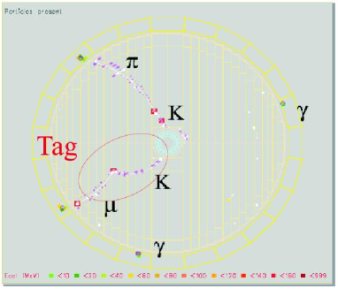
Figure 46: Display showing a K⁺K^-event selected exploiting the tagging.

As previously said, the tagging allows us to select samples of K⁺K^-and of K${}^{0}_{S}$K${}^{0}_{L}$. Thus the strategy for the selection of $K_{l3}$ decays is: tag with one kaon of the pair and look for the desired semileptonic decay of the other.

The very clean signature of the decays K${}^{\pm}\rightarrow\pi^{\pm}\pi^{0}$ and K${}^{\pm}\rightarrow\mu^{\pm}\bar{\nu}(\nu)$ is exploited to tag charged kaons, while K${}^{0}_{S}\rightarrow\pi^{+}\pi^{-}$ decays tag the K${}^{0}_{L}$neutral kaon (fig. 46). Only drift chamber information is used in both cases. The tagging efficiencies can be estimated directly from data. For charged kaons we use the redundant calorimetric information of the K${}^{\pm}\rightarrow\mu^{\pm}\bar{\nu}(\nu)$ events while for the tagging provided by K${}^{0}_{S}\rightarrow\pi^{+}\pi^{-}$  we use the sample of K${}^{0}_{L}$ interacting in the Electromagnetic Calorimeter.

With the statistics of $\sim 500\textrm{pb}^{-1}$ we can reach a level of $O(0.07\%)$ accuracy on tagging efficiencies.

The sample of $K^{\pm}_{l3}$ events is selected asking for a tag on one side and on the other for a vertex in the drift chamber and one $\pi^{0}$ in the electromagnetic calorimeter. The time of flight information separates charged pions from electrons, exploiting the excellent timing resolution of the detector. From preliminary studies we expect the number of $K^{\pm}_{e3}$ decays to be $N_{K^{\pm}_{e3}}\simeq 2000/\textrm{pb}^{-1}$, which means a total number of $N_{K^{\pm}_{e3}}\simeq 10^{6}$, after analysis cuts. Most of the selection efficiencies can be evaluated directly from data using control samples, a method already used in the measurement of $\Gamma(K_{S}\to\pi^{+}\pi^{-}(\gamma))/\Gamma(K_{S}\to\pi^{0}\pi^{0})$ ksrapp . The momentum range of the lepton in $K^{\pm}_{l3}$ is covered by K${}^{\pm}\rightarrow\pi^{\pm}\pi^{0}$  K${}^{\pm}\rightarrow\mu^{\pm}\bar{\nu}(\nu)$ and K${}^{\pm}\rightarrow\pi^{\pm}\pi^{0}\pi^{0}$ decays (fig. 47). The energy range of the most energetic cluster of the $\pi^{0}$ from the semileptonic decay is covered by K${}^{\pm}\rightarrow\pi^{\pm}\pi^{0}$ and K${}^{\pm}\rightarrow\pi^{\pm}\pi^{0}\pi^{0}$ decays (fig. 47).

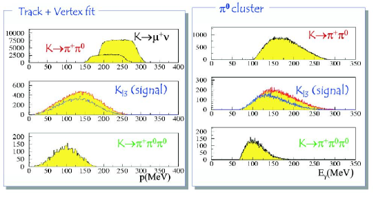
Figure 47: Distribution of the momentum of the lepton (left) and of the energy of the most energetic cluster of the $\pi^{0}$ (right) for $K^{\pm}_{l3}$ decays and for the control samples K${}^{\pm}\rightarrow\pi^{\pm}\pi^{0}$  K${}^{\pm}\rightarrow\mu^{\pm}\bar{\nu}(\nu)$ and K${}^{\pm}\rightarrow\pi^{\pm}\pi^{0}\pi^{0}$ decays.

The sample of $K^{0L}_{l3}$ events is selected asking for a tag on one side and on the other asking for a vertex in the drift chamber fiducial volume, applying a cut on the invariant mass. The time of flight information separates pions from muons and electrons. The total number of semielectronic K${}^{0}_{L}$ decays is $N_{K^{0L}_{e3}}\sim 1.5\times 10^{6}$, after analysis cuts. This procedure has been already used in the measurement of the branching ratio of K${}^{0}_{S}\rightarrow\pi^{\pm}e^{\mp}\bar{\nu}(\nu)$ decay kssemil .

Moreover at KLOE we can improve the actual measurements on the vector form factor slope $\lambda_{+}$, using both charged and neutral $K_{e3}$ decays. With the present data sample we can reach a statistical accuracy of $O(10^{-4})$ for $\lambda^{+}$ from $K^{0}_{e3}$ and of $O(10^{-3})$ using $K^{\pm}_{e3}$, values which are competitive with the ones of the actual measurements.

Conclusions

The KLOE experiment can improve the actual situation of the $V_{us}$ CKM-matrix element measuring, with the same detector, the absolute branching ratios both for charged and neutral kaon semileptonic decays and measuring directly the partial decay widths. Moreover the accuracies that can be reached are beyond the present theoretical ones. Therefore KLOE can give a unique contribution in understanding the SU(2) and SU(3)_F symmetry breaking effects and the radiative corrections applied to the decay rates in order to determine the value of $V_{us}$.

*An Ultracold Neutron Facility at PSI
An Ultracold Neutron Facility at PSI M. Daum for the PSI-PNPI-ILL-Cracow-IMEP UCN Collaboration M. Daum

78 The New UCN Source

A new type of ultra-cold neutron source (SUNS, Spallation Ultra-cold Neutron Source) based on the spallation process is under construction at PSI. A detailed description of the source parameters can be found in Ref. tm . The essential elements of SUNS are a pulsed proton beam with highest intensity (I${}_{p}\geq$ 2 mA) and a low duty cycle ($\sim$ 1 %), a heavy-element spallation target, and a large moderator and converter system consisting of about 4 m³ of heavy water at room temperature and 30 dm³ of solid deuterium (SD₂) kept at a low temperature ($\sim$ 6 K) for the production of ultra-cold neutrons. Operating the UCN source in a pulsed mode will allow maintaining the SD₂ at very low temperatures despite of the large temporary heat load deposited in the spallation target. The proton beam is directed onto the neutron production target for a few seconds only, a time long enough to fill the intermediate UCN storage vessel ($\sim$ 2 m³). A high neutron density is generated in the moderator assembly. The neutrons are thermalized in the D₂O, further cooled in the SD₂ and finally, some of them are down-scattered into the ultra-cold neutron range (T${}_{\mbox{kin}}\leq 250$ neV).

About when equilibrium between the produced and re-absorbed UCNs is achieved in the storage volume, the SD₂ moderator is separated from the latter by a reflective shutter, in order to prevent re-absorption of the UCNs in the cold moderator. The proton beam is turned off, and the UCNs are transferred from the storage volume to the EDM apparatus. The filling of the source storage volume is repeated after about 800 s, i.e., as soon as the UCN density in the storage volume has dropped significantly. The source layout, pulse duration, and storage volume are optimized for a dedicated EDM spectrometer of about 0.2 m³ volume.

Monte Carlo calculationstm show that at this source, an average UCN density of $\sim$ 3$\cdot 10^{3}$ UCN/cm³ can be delivered to the experiments. This is about two orders of magnitude more than in the present experiments at the reactors in the Institute Laue Langevin, ILL, Grenoble and in the St. Petersburg Nuclear Physics Institute, PNPI, Gatchina. This average UCN density corresponds to a pulsed proton beam current I_p = 2 mA (600 MeV) with a pulse duration of 8 seconds and a 1 % duty cycle. The target material assumed for this calculation is lead with a filling factor (Pb/D₂O ratio) of 0.5.

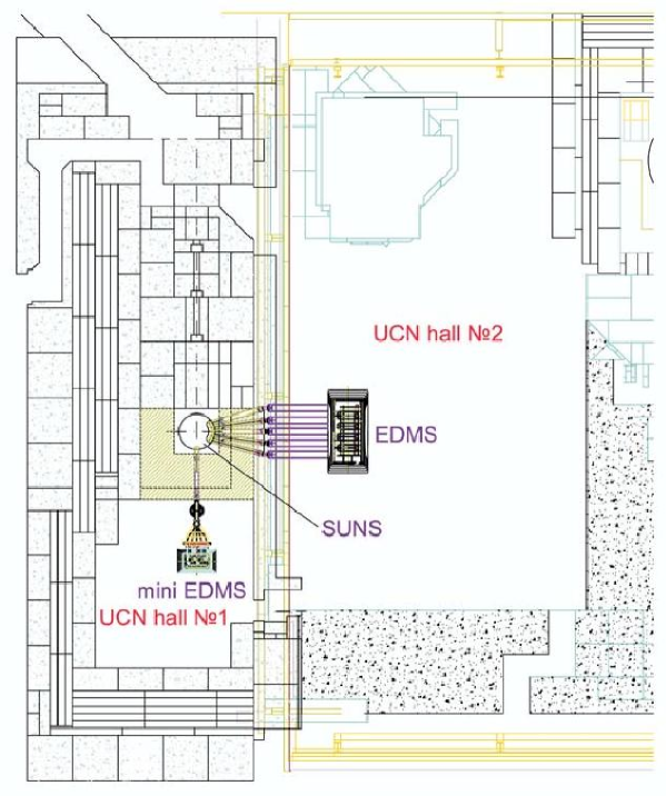
Figure 48: Layout of SUNS and EDM spectrometers in the different experimental areas at PSI.

The new UCN facility at PSI will be built in two steps. The layout of SUNS and the connected experimental areas are shown in Fig. 48. In 2006, the source is expected to be operational and a first experimental area will be available for experiments with UCNs (mini EDMS, UCN hall No.1, Fig. 48). At a later stage ($\sim$2007-2008), an extended area (EDMS, UCN hall No.2, Fig. 48) will complete the experimental installations at this facility. Then, a second step of an EDM Experiment with an EDM spectrometer of highly increased volume ($\sim$0.2 m³) as well as various other fundamental experiments can be envisaged.

*Three-fold Correlation in the Interaction
of Polarized Neutrons with Polarized Nuclei
and the Method of Oscillating Fields
Three-fold Correlation in the Interaction of Polarized Neutrons with Polarized Nuclei and the Method of Oscillating Fields A.V.Aldushchenkov, A.I.Kovalev, V.V.Lukashevich

There is an intriguing problem of searching for breaking T-invariance in the low energy physics. One of the possible variants of such searching has been under discussion nearly for recent 20 years. This is a study of the slow neutrons interaction with ¹³⁹La. An interest to this nucleus is stipulated by the fact that closely lying s,p-resonances created in a compound state by passing neutrons could enhance the T-violation interaction on 5-6 orders.

P,T–odd interaction in ¹³⁹La is like the interaction of an axial neutron dipole moment with an electric field but it seems more attractive because of large enhancement factor. T–odd, P–even interaction is phenomenological and is not followed by the extension of standard model, though such an interaction is studied carefully in five-fold correlation journ1 .

Traditionally, the amplitude of interaction of neutrons with a nucleus is written as

$$f=A+p_{t}B(\vec{s}\vec{I})+C(\vec{s}\vec{k})+p_{t}D(\vec{s}[\vec{k}\vec{I}]),$$

where I - spin nucleus, $p_{t}$- target polarization, s - neutron spin and k - its wave vector.

The experimental measurement subject is a value T–violation amplitude $D$. The hierarchy spin depended forces is such as $B\gg C\gg D$, so it is difficult to separate the small P,T-odd effect from the large background effects of strong, electromagnetic and helicity depended neutron-nucleus interactions.

There are several proposals how to measure the value of $D$ journ2 . However, according to analysis journ2 and journ3 , some of them are practically unattainable, while some others are wrong. So, new presentations are required to resolve a problem under discussion.

In the given work the possibility of T-breaking amplitude measurement is discussed on the basis of a high sensitive method of magnetic exact, two coil method by Ramsey journ4 .

A neutron spin is parallel to the magnetic field H and a nuclear polarization at the entrance of the first coil. After a coil the spin is turned on $\frac{\pi}{2}$. Then, a neutron goes through the target and the second coil, in which the spin is turned on $\frac{\pi}{2}$ once more, and an analyzer measures its polarization.

A result of polarized neutron interaction with the efficient pseudomagnetic, weak P-odd and T-violation fields in the polarized target is convenient to describe within the framework of the density matrix formalism. This enables one to define an experimental strategy.

Let us use a standard presentation for the density matrix

$$\rho=\frac{1}{2}[1+(\vec{p}\vec{\sigma})],$$

where $\vec{p}$ is the neutron polarization vector and $\vec{\sigma}$ are the Pauli matrices. For neutrons, polarized along axis z, the matrix of density is diagonal and the components of polarization vector are $p_{z}=p_{0}$, $p_{x}=p_{y}=0$. The passing of neutrons through the first coil with the radio-frequency field, target and second coil in terms of the density matrix is described as follows

$$\rho=U_{2}U_{int}U_{1}\rho_{0}U_{1}^{\dagger}U_{int}^{\dagger}U_{2}^{\dagger}.$$ (203)

In this expression $U_{1}$, $U_{2}$are the time evolution operators for the first and second coils, accordingly. $U_{int}$ is the evolution operator, describing a transformation of density matrix by the interaction in a target. $\rho_{0}$ is an initial density matrix. On condition that the field frequency in coils is equal to the frequency of Larmor precession in the external magnetic field and that the spin turning angle is equal to $\frac{\pi}{2}$ in each of the coils, the Hamiltonian of a neutron in the coils in the rotating coordinate system has a simple type

$$H_{1}=H_{2}=\frac{\pi}{4}(\vec{n}\vec{\sigma}).\\$$

Here $\vec{n}$ is a single vector toward the magnetic field. For specified conditions, this vector has following components: $n_{z}=0$, $n_{x}=\cos\delta$, $n_{y}=\sin\delta$,

where $\delta$ is a random phase, with which a neutron flies in the first coil.

After passing first coil, a density matrix becomes equal to

$$\rho_{1}=\frac{1}{2}[1+p_{0}(\sigma_{x}\sin\delta-\sigma_{y}\cos\delta)].$$ (204)

That is to say, neutron spins ”lie” in horizontal plane and a spin direction is defined by the initial phase $\delta$. For the density matrix evolution of neutrons in the polarized target ¹³⁹La we will use the results of work journ3 , in which general solution for the density matrix

$$\rho_{int}=U_{int}\rho_{1}U_{int}^{\dagger}$$ (205)

is given with a free matrix $\rho_{1}$.

Let us suppose that a vector of target polarization and an external magnetic field are directed along the axis z and neutrons are moved along the axis y. Then, using (205), (204) and (203) we find expression for matrix on the device exit, which in the expanding form is

$$\rho=\frac{1}{2}[N_{0}+(\vec{P}\vec{\sigma})],$$ (206)

where

$$P_{z}=-p_{x}^{{}^{\prime}}\sin\delta_{1}+p_{y}^{{}^{\prime}}\cos\delta_{1},$$

$$P_{x}=\cos\delta_{1}(p_{x}^{{}^{\prime}}\cos\delta_{1}+p_{y}^{{}^{\prime}}\sin\delta_{1})+p_{z}\sin\delta_{1}$$

$$P_{y}=\sin\delta_{1}(p_{x}^{{}^{\prime}}\cos\delta_{1}+p_{y}^{{}^{\prime}}\sin\delta_{1})-p_{z}\cos\delta_{1}.$$

The phase $\delta_{1}$contains a constant difference $\epsilon$ between the radio frequency phases of the two coils, so that $\delta_{1}=\delta+\epsilon$.
In (206) $p_{i}^{{}^{\prime}}$ are projections of the polarization vector after the target, which are defined in journ3 . From this work we also take the determination of efficient fields. The vector $\vec{b}^{{}^{\prime}}=\frac{\sin{qt}}{q}\vec{b}$, where $q=\sqrt[2]{\vec{b}\vec{b}}$ and the vector $\vec{b}$ is a resulting vector of the three fields, which a neutron interacts with and $qt$ is the efficient angle of neutron spin rotation around this vector.

In the chosen coordinate system values $b_{i}^{{}^{\prime}}$ are connected with efficient fields in a target as follows

• the T violation field $b_{x}=p_{t}\frac{D}{2}$,

• the field of weak interaction $b_{y}=\frac{C}{2}$,

• and the so called pseudomagnetic field $b_{z}=p_{t}\frac{B}{2}$.

Here $p_{t}$ is the target polarization factor.

A general form of the density matrix (206) allows us to construct three asymmetries. The first is an asymmetry depended on the neutron phase, the second – on the neutron polarization and the third - on a degree of the target polarization. However, under detailed consideration, two last asymmetries do not allow to select T- violation amplitude D, so we will give an analysis of the asymmetry of neutron polarization $\eta_{\delta}$ depending on a neutron phase. The final result for $\eta_{\delta}$ is

$$\eta_{\delta}=\frac{\rho_{11}(\delta)-\rho_{11}(-\delta)}{\rho_{11}(\delta)+\rho_{11}(-\delta)}=\frac{E}{F},$$ (207)

where $\rho_{11}$ is the matrix element of the density matrix (206).

$$E=4\sin{\delta}[(p_{0}+\cos{\epsilon})Im(b_{y}^{{}^{\prime}}b_{z}^{{}^{\prime}\ast})+(p_{0}-\cos{\epsilon})Im(b_{x}^{{}^{\prime}\ast}\cos{qt})$$

$$+2p_{0}\cos{\delta}\cos{\epsilon}Re(b_{x}^{{}^{\prime}}b_{y}^{{}^{\prime}\ast})]+4\sin{\delta}\sin{\epsilon}[p_{0}\cos{\delta}(|b_{y}^{{}^{\prime}}|^{2}-|b_{x}^{{}^{\prime}}|^{2})$$

$$-Im(b_{x}^{{}^{\prime}}b_{z}^{{}^{\prime}\ast}-b_{y}^{{}^{\prime}\ast}\cos{qt})]$$

$$F=2[(1+p_{0}\cos{\epsilon}\cos{2\delta})|b_{x}^{{}^{\prime}}|^{2}+(1-p_{0}\cos{\epsilon}\cos{2\delta)}|b_{y}^{{}^{\prime}}|^{2}+(1+p_{0}\cos{\epsilon})|b_{z}^{{}^{\prime}}|^{2}$$

$$+(1-p_{0}\cos\epsilon)|\cos{qt}|^{2}]+4\cos{\delta}(p_{0}+\cos{\epsilon})Im(b_{x}^{{}^{\prime}}b_{z}^{{}^{\prime}\ast})$$

$$-4\cos{\delta}(p_{0}-\cos{\epsilon})Im(b_{y}^{{}^{\prime}\ast}\cos{qt})$$

$$+4\sin{\epsilon}[\cos 2{\delta}Re(b_{x}^{{}^{\prime}}b_{y}^{{}^{\prime}\ast}+p_{0}Re(b_{z}^{{}^{\prime}\ast}\cos{qt})-\cos{\delta}(Im(b_{y}^{{}^{\prime}\ast}b_{z}^{{}^{\prime}}+Im(b_{x}^{{}^{\prime}\ast}\cos{qt}))].$$

We can choose the instrumental phase $\epsilon$ equal to $\pi$ and take $p_{0}=1$ because the polarization degree of neutron beams is approximately equal to 1 in real experiments. Under these conditions the expression (207) is significantly simplified

$$\eta_{\delta}=\frac{2\sin{\delta}[Im(b_{x}^{{}^{\prime}\ast}\cos{qt})-\cos{\delta}Re(b_{x}^{{}^{\prime}}b_{y}^{{}^{\prime}\ast})]}{\sin^{2}{\delta}|b_{x}^{{}^{\prime}}|^{2}+\cos^{2}{\delta}|b_{y}^{{}^{\prime}}|^{2}+|\cos{qt}|^{2}-2\cos{\delta}Im(b_{y}^{{}^{\prime}}\cos{qt})}.$$ (208)

Now this is a critical point of the analysis. In (208) for the quantity $q$ we can take into account only the large term corresponding to the pseudomagnetic field then

$$q=ReB+iImB.$$

Let us re-write (208) in terms of efficient fields saving only main values and neglecting the second term in the numerator (208) as far as it has the second order of smallness.

As it is pointed out by Abragam mono2 $ImB\sim 10^{-3}ReB$. It allows us not to include terms with $ImB$. After these remarks we have

$$\eta_{\delta}\approx p_{t}\frac{4\sin{\delta}ImD}{{\omega}ctg{\frac{{\omega}t}{2}}+4\cos{\delta}ImC},$$ (209)

where $\omega=ReB$ is the frequency of neutron spin precession in pseudomagnetic field.

We can evaluate this frequency from pseudomagnetic moment ¹³⁹La which was measured in journ5 . The pseudomagnetic field in crystal LaAlO₃(Nd³⁺) is found less than 1kG at the target polarization 50%. The spin makes several turns in this field for the flight time ($10^{-6}$ sec) through the target with length 1cm. We can notice that such level of polarization in crystal LaAlO₃(Nd³⁺) was reached in the work journ6 .

The P,T-odd effect shown by Eq. (209) disappears in the case when the spin makes the integer number of turns and the effect is maximum when the complete precession angle is different on ${\pi}$ from the integer number of turns. The second opportunity may be realized by the corresponding choice of the target length for neutrons with p-wave resonance energy 0.734eV. From the expression (209) follows that the phase analysis have not to be done near phase angle $\delta=0,{\pi}$.

As a result, it is possible to conclude that the experimental found asymmetry (209) can be a measure of breaking T-invariance at the interaction of slow neutrons with nuclei.

In the experimental plan the measurement of the $\eta_{\delta}$ value means a synchronization moment of a neutron registration in the counter (after passing an analyzer) with the phase of radio frequency field and a selection of events with phases distinguishing on $\pi$. More exactly, neutrons with the energy of p-wave resonance $E_{n}=0.734eV$ are registered as function of phase $\delta$. On the basis of the existing technique, the accuracy of phase angle measurements can be order of one degree journ7 .

*Trine – A New Limit on Time Reversal Invariance Violation in Neutron $\beta$-Decay Trine – A New Limit on Time Reversal Invariance Violation in Neutron $\beta$-Decay T. SoldnerL. BeckC. PlonkaK. SchreckenbachO. Zimmer

79 Introduction

To create the baryon antibaryon asymmetry in the universe from a symmetric start, a baryon number, C and CP violating process outside thermal equilibrium is required sakharov1967 . CP violation was discovered in the decay of neutral kaons christenson1964 . This type of CP violation is implemented in the Standard model of particle physics via a free phase in the quark mixing matrix kobayashi1973 but seems to be insufficient to explain the observed baryon asymmetry herczeg2001 .

Extensions of the Standard model like SUperSYmmetric models or Grand Unified Theories open new channels for CP violation which may be observed in low energy particle physics like in electric dipole moments (EDMs) or in the neutron beta decay. Especially the neutron EDM is a sensitive test for physics beyond the Standard model and restricts the parameter space for many alternative models ellis1989 . The decay, however, namely the triple correlation $D$ of the spin of the decaying neutron and the momenta of electron and antineutrino, is more sensitive for CP violation via leptoquarks herczeg2001 which appear naturally in GUTs.

The differential decay probability of the neutron can be written as jackson1957a :

$$\frac{{\rm d}W}{{\rm d}E_{\rm e}{\rm d}\Omega_{\rm e}{\rm d}\Omega_{\bar{\nu}}} = gG_{\rm E}(E_{\rm e})\left\{1+a\frac{\vec{p}_{\rm e}\vec{p}_{\bar{\nu}}}{E_{\rm e}E_{\bar{\nu}}}+b\frac{m_{\rm e}}{E_{\rm e}}+\right.$$

$$\left.\frac{\vec{\sigma}_{\rm n}}{\sigma_{\rm n}}\left(A\frac{\vec{p}_{\rm e}}{E_{\rm e}}+B\frac{\vec{p}_{\bar{\nu}}}{E_{\bar{\nu}}}+D\frac{\vec{p}_{\rm e}\times\vec{p}_{\bar{\nu}}}{E_{\rm e}E_{\bar{\nu}}}\right)\right\}$$

Here, $g$ is a normalization constant, $G_{\rm E}$ the electron spectrum, $\vec{\sigma}_{\rm n}$ the neutron spin, $E_{i}$ the energy, $\vec{p}_{i}$ the momentum, and ${\rm d}\Omega_{i}$ the solid angle of electron e and antineutrino $\bar{\nu}$, respectively. The coefficients $a$, $b$, $A$, $B$, and $D$ describe the correlations between the decay products.

Eq. (79) assumes only Lorentz invariance but no discrete symmetries like parity P, charge conjugation C, or time reversal T. Indeed, the coefficients $A$ and $B$ are P and C violating and nonzero ($A=-0.1162(13)$, $B=0.983(4)$ pdg2002 ). In the V–A-theory $A$ or $a$ are used to determine the ratio $|\lambda|:=|g_{\rm A}/g_{\rm V}|$ of the axial vector and the vector coupling constant ($b\equiv 0$ in V–A-theory). Together with the neutron life time the absolute values of the coupling constants can be determined. For a precise measurement of the phase of $\lambda$, however, the $D$ coefficient is required. A phase $\neq 0,\pi$, i.e. $D\neq 0$, would indicate T violation (and according to the CPT theorem CP violation). Up to now, no evidence for a deviation of $D$ from 0 was found (world average $D=-0.6(1.0)\cdot 10^{-3}$ pdg2002 ). The Standard model prediction is $D<10^{-12}$. Any value above the final state effect level ($D_{\rm FS}\approx 10^{-5}$ for neutrons) would indicate new physics. For leptoquark models, this experimental range is not excluded by measurements of alternative parameters (like, e.g., EDMs) herczeg2001 .

80 Principle of a $D$ measurement

To measure $D$ in neutron decay, electron and proton (which can replace the antineutrino for slow neutrons) have to be detected dependent on the neutron spin. Integrating (79) over the acceptance of electron detector $i$ and proton detector $j$ gives the count rate $\dot{N}^{ij}$ of the detector combination ${\rm e}^{i}{\rm p}^{j}$:

$$\dot{N}^{ij}=\epsilon_{\rm e}^{i}\epsilon_{\rm p}^{j}\left\{K_{1}^{ij}+aK_{a}^{ij}+bK_{b}^{ij}+\vec{P}\left(A\vec{K}_{A}^{ij}+B\vec{K}_{B}^{ij}+D\vec{K}_{D}^{ij}\right)\right\}.$$ (211)

Here, $\epsilon_{\rm e}^{i}$ ($\epsilon_{\rm p}^{j}$) describes the detector efficiency of electron (proton) detector $i$ ($j$). $K_{\eta}^{ij}$ are apparatus constants that describe the sensitivity of the apparatus versus the coefficient $\eta\in\{1,a,b,A,B,D\}$, e.g.

$$K_{1}^{ij}\propto\left\langle\int_{{\rm e}^{i}{\rm p}^{j}}G_{\rm E}(E_{\rm e}){\rm d}E_{\rm e}{\rm d}\Omega_{\rm e}{\rm d}\Omega_{\bar{\nu}}\right\rangle_{V}$$

   or   

$$\vec{K}_{D}^{ij}\propto\left\langle\int_{{\rm e}^{i}{\rm p}^{j}}G_{\rm E}(E_{\rm e})\frac{\vec{p}_{\rm e}\times\vec{p}_{\bar{\nu}}}{E_{\rm e}E_{\bar{\nu}}}{\rm d}E_{\rm e}{\rm d}\Omega_{\rm e}{\rm d}\Omega_{\bar{\nu}}\right\rangle_{V}.$$

$\langle\ldots\rangle_{V}$ represents the average over the decay volume. $\vec{P}$ is the neutron polarization. Modifications are necessary for inhomogeneous $\epsilon$ or $\vec{P}$. The $K_{\eta}$ can be determined by Monte Carlo simulations. The quotient

$$\alpha^{ij}:=\frac{\dot{N}^{ij}_{\uparrow}-\dot{N}^{ij}_{\downarrow}}{\dot{N}^{ij}_{\uparrow}+\dot{N}^{ij}_{\downarrow}}=\vec{P}\left(A\vec{\kappa}_{A}^{ij}+B\vec{\kappa}_{B}^{ij}+D\vec{\kappa}_{D}^{ij}\right)$$ (212)

with $\vec{\kappa}_{\eta}^{ij}=\vec{K}_{\eta}^{ij}/(K_{1}^{ij}+aK_{a}^{ij}+bK_{b}^{ij})$ is independent on detector efficiencies.

Since $D\ll A,B$ the influence of the parity violating coefficients $A$ and $B$ has to be suppressed carefully. Therefore, the detector and the decay volume should have two common perpendicular mirror planes ($x$-$z$ and $y$-$z$ planes in Fig. 49 (a) which shows the simplest implementation). For such detector, $A$ and $B$ are suppressed to first order:

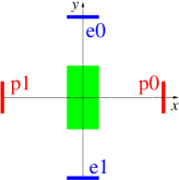
(a)     (b)    

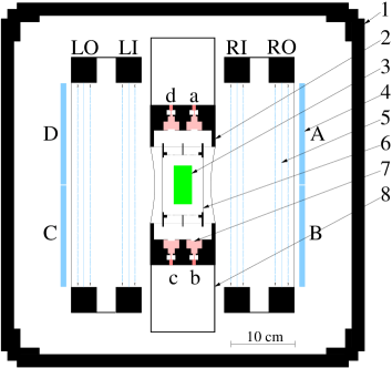
Figure 49: (a) Simplest symmetric detector for $D$, (b) Cross section of the Trine detector: 1 – outer chamber (counting gas), 2 – inner vacuum chamber, 3 – neutron beam, 4 – plastic scintillator, 5 – wire chamber, 6 – electrode for proton acceleration, 7 – PIN diode, 8 – housing for PIN preamplifier. For both detectors, the polarizations points in $z$ direction perpendicular to the plane of the drawing.

$$4P_{z}\kappa_{D,z}D=\alpha^{00}-\alpha^{01}-\alpha^{10}+\alpha^{11}=:\alpha_{D}.$$ (213)

This bases on the different symmetry properties of $\vec{\kappa}_{A}\propto\vec{p}_{\rm e}$, $\vec{\kappa}_{B}\propto\vec{p}_{\bar{\nu}}$, and $\vec{\kappa}_{D}\propto\vec{p}_{\rm e}\times\vec{p}_{\bar{\nu}}$. The detector is insensitive to a beam divergence and to deviations of the polarization from $z$ axis. However, deviations from the mirror symmetries are sources for systematic errors. Whereas (213) suppresses the influences of the parity violating coefficients one can define asymmetries that enhance this influence and allow to investigate imperfections of the set-up:

$$\alpha_{x}:= \alpha^{00}+\alpha^{01}-\alpha^{10}-\alpha^{11} =4P_{x}(A\kappa_{A,x}+B\kappa_{B,x})+4P_{y}D\kappa_{D,y}$$ (214)

$$\alpha_{y}:= \alpha^{00}-\alpha^{01}-\alpha^{10}+\alpha^{11} =4P_{y}(A\kappa_{A,y}+B\kappa_{B,y})+4P_{x}D\kappa_{D,x}$$ (215)

$$\alpha_{z}:= \alpha^{00}+\alpha^{01}+\alpha^{10}+\alpha^{11} =4P_{z}(A\kappa_{A,z}+B\kappa_{B,z}).$$ (216)

The index of these combined asymmetries indicates the component of the polarization the asymmetry is sensitive to (cf. Fig. 49 (a)). In principle, (214)-(216) allow to derive the full polarization vector from the measured combined asymmetries, using the values for $A$ and $B$ from literature.

A further reduction of the sensitivity to the coefficients $A$ and $B$ can be obtained by optimizing the angle $\varphi$ between electron and proton detector. This sensitivity can be described by $\kappa_{A}(\varphi)/\kappa_{D}(\varphi)$ and $\kappa_{B}(\varphi)/\kappa_{D}(\varphi)$ and has a minimum at slightly obtuse angles of about 120^∘, depending on the specific detector dimensions soldner2000a .

The statistical sensitivity of a combination of electron and proton detector is determined by the angular correlation between electron and proton and the dependence $\kappa_{D}=\kappa_{D}(\varphi)$ and has its maximum at about 135^∘ lising2000 ; soldner2000a .

81 The Trine Experiment

Trine detects the electrons by 4 plastic scintillators ($560\times 158\times 8.5$ mm³) in coincidence with multi wire proportional chambers and the protons after acceleration in a focusing electrostatic field by special PIN diodes with thin entrance windows (diameter of active area 10 mm, 25 nm dead layer; see beck1997 for the performance). Fig. 49 (b) shows a cross-section of the detector. The detector consists of 16 such planes which use the same four scintillators and wire chambers (Fig. 50). Only the central detector planes 03–14 and plane 16 were equipped with PIN diodes. Data analysis used the 12 central planes to avoid edge effects at the ends of the high voltage electrode. Plane 16 served to investigate these effects.

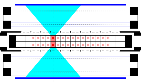
Figure 50: Top view of the detector, symmetrization: The electron has to pass the wire chamber in a range symmetric to the PIN diode plane hit by the proton.

In each plane, four groups of detector combinations exist defined by the enclosed angle between electron and proton detector: 50^∘, 82^∘, 98^∘, and 130^∘. Each group fulfills the symmetries requested in section 80 (Fig. 49).

The experiment was carried out at the ILL cold neutron beam facility PF1. The beam polarization of $P=0.974(26)$ was created by a focusing polarizer. The neutron spin was flipped every 3 s by a resonance flipper. An octagonal long coil (length 180 cm, diagonal 96 cm, correction coils at the ends), surrounded by a mu metal tube to shield the earth magnetic field, created the longitudinal spin holding field of 140 $\mu$T in the detector region. The field deviation $B_{\perp}/B_{z}$ from the $z$ axis was smaller than $5\cdot 10^{-3}$.

The neutron beam profile was measured at the beginning, the center and the end of the decay volume ($z=-15,0,15$ cm respectively) using gold foils which were exposed to the neutron beam and than scanned with an image plate soldner2000a . The profile is slightly inhomogeneous in $y$ direction (Fig. 51), caused by an inhomogeneous transmission of the focusing polarizer.

Figure 51: Cuts of the beam profile (capture flux) in the decay volume in $y$ direction. The solid lines correspond to 2 dimensional Fourier expansions of the data. The decay rate from this flux is about $10^{3}$/s in the detector volume, resulting in a count rate of about 10/s (due to solid angle and electron-proton correlation).

Data acquisition required the coincidence of a scintillator and the corresponding outer wire chamber. Thus, the trigger rate for events to store was kept low. Events without a wire chamber signal contributed a dead time of only 1.2 %. For each event, the analog signals of all scintillators, the numbers of the wires hit in all wire chambers, the number(s) and analog value(s) of the PIN diode(s) hit in the 10 $\mu$s after the second trigger, and the proton time of flight (TOF) between trigger and the first PIN diode hit were registered by a VME based acquisition system. The dead time per stored event was 30 $\mu$s, resulting in an overall dead time of 3.3 %. The VME bus was read out synchronously with the spin flip. Incomplete events (i.e. events without proton signal within the 10 $\mu$s) were sorted out by software. Only every 16th incomplete event was saved for control purposes. Monitor data like neutron flux, count rates of single detectors, high voltages of the electrode and the wire chambers were stored for each spin interval.

From the 100 days available at PF1 about 25 days in the first and 40 days in the second reactor cycle were used to collect statistics and 10 days of the second cycle for systematic tests. During the measurement, the scintillators were recalibrated every 10 days but only small adjustments were needed. Data from the first cycle suffered from high voltage problems and are not analysed yet. In the following we present the analysis of the data from the second cycle.

82 Data Analysis

82.1 Selection of events

Spin intervals with unusual values of monitor signals together with the following three intervals and spin intervals where one VME module lost a trigger were removed (approx. 4 %). Only complete events with exactly one triggering PIN diode were used. A threshold of 150 keV was applied to the electron signal by software (hardware threshold was about 115 keV). The stability of the detectors was verified by an automatic generation of software cuts to the PIN analog spectra and allowed to sum the data to 10 days samples, corresponding to the period of scintillator recalibrations.

Figure 52: Typical TOF spectrum (1 PIN diode and 1 scintillator for 98^∘). The dashed lines indicate the ranges for the background fit, the solid line the fit result.

Individual TOF spectra were calculated for all detector combination in each sample using the events that fulfill the software cuts. The background of the TOF spectra was fit by an exponential in a fixed range before and after the coincidence peak (Fig. 52). This shape of the background follows from the data acquisition which stopped the TOF measurement with the first proton signal. As a further consequence, the background behind the peak is suppressed compared to that in front of it. The $\chi^{2}$ analysis showed perfect agreement between the exponential and the data for separate fits of the two fit ranges but a systematic increase to $\chi^{2}/{\rm ndf}=1.26$ (averaged over all individual spectra) for a common fit of the ranges. To account for this the error of the background was scaled by a factor 1.124, but anyway the effect is very small due to the excellent signal to background ratio of 23 (averaged over the detector combinations used). The thus obtained peak areas were normalized with the neutron monitor counts of the particular spin to account for fluctuations caused by upstream experiments.

82.2 Selection of Detector Combinations

The measured count rates of the detector combinations 50^∘ and 82^∘ were higher than expected from the Monte Carlo simulations. These combinations are more sensitive to systematic effects due to the small particle energies caused by kinematics. This increases the scattering for electrons (e.g. by the counting gas). The low energy protons may be disturbed by a small penetration of the electrostatic field into the electrode. Furthermore, the sensitivity to $A$ and $B$ coefficient is larger for angles below 90^∘ than for slightly obtuse angles, and the contribution of small angle combinations to the statistics can be neglected (see section 80 or soldner2000a ). Therefore, only the larger angle combinations (98^∘ and 130^∘) were used in the analysis.

82.3 Detector “Symmetrization”

The single asymmetry $\alpha^{ij}$ of a detector combination close to an end of the decay volume is high due to the spatial asymmetry of this combination in $z$ direction, resulting in a sensitivity to $A$ and $B$ (Fig. 53, top). This sensitivity cancels by calculating the combined asymmetry $\alpha_{D}$ (section 80). However, for a real detector, effects like inhomogeneous detector efficiencies result in an incomplete cancellation which can fake $D\neq 0$.

Figure 53: Combined asymmetries $\alpha_{z}\approx 4\alpha$ as function of the detector plane. Top: full scintillator, Bottom: symmetrized detector with $\pm 10$ cm per plane.

The spatial resolution of the wire chamber was used to suppress this sensitivity already in the initial asymmetries by selecting a symmetric electron detector range for each detector plane (see Fig. 50). The resulting asymmetries $\alpha_{z}$ are plotted in Fig. 53 (bottom). The size of the range was selected such that the variations of $\alpha_{D}$ between the different planes were consistent with statistical variations. For $\pm 10$ cm a $\chi^{2}$ of 10.4 (12.2) for 11 degrees of freedom was found for 98^∘ (130^∘). The slightly higher $\chi^{2}$ for 130^∘ was taken into account as a systematic error of $2.2\cdot 10^{-4}$. The change of the $\alpha_{D}$ values for different sizes of the wire chamber range was not fully compatible with statistics. Although this is expected since the range serves to suppress systematic effects it was considered as a contribution to the systematic error of $1.0\cdot 10^{-4}$ by comparing the $D$ values for different wire range sizes.

82.4 Influence of the Beam Profile

The influence of the beam profile was investigated with test measurements where one half or one quarter of the polarizer exit were closed to increase the beam shift (center of mass shifted by $\Delta y=7.2$ mm for the 3/4 beam compared to 1 mm for the full beam). The results $D_{\rm 3/4}$ for the both detector combinations used were consistent with 0 but were used to limit the systematic error caused by the inhomogeneous beam profile: $\delta_{\rm shift}D=16(13)\cdot 10^{-4}$ ($2.4(5.0)\cdot 10^{-4}$) for 98^∘ (130^∘) (statistical error given). A more precise calculation of this systematic error by Monte Carlo simulations is in progress and will replace the present estimation in the final result.

82.5 Results and Outlook

During the second cycle, $30\cdot 10^{6}$ events were collected with the unshifted beam. $13.8\cdot 10^{6}$ events fulfilled the symmetry condition (wire chamber range). The preliminary result is $D=(-3.1\pm 6.2^{\rm stat}\pm 4.7^{\rm syst}\pm 4.7^{\rm syststat})\cdot 10^{-4}$. Syststat indicates the statistical error of the systematic error determined with the partially covered beam and will not enter into the final result after the Monte Carlo simulations (section 82.4). The systematic error consists of the contributions given in sections 82.3 and 82.4 and those from the uncertainties of the apparatus constants ($0.3\cdot 10^{-4}$) and polarization ($0.08\cdot 10^{-4}$).

Table 14: Comparison of the latest $D$ measurements.

Year $P$ Events Sig/BG $D$ $[\%]$ $[10^{6}]$ $[10^{-3}]$ steinberg1976 1976 70 (7) 6 4 –1 .1 $\pm$1.7 erozolimskii1978 1978 68 (3), 65(1) 2 .5 2 .2 2 .2 $\pm$3.0 emiT lising2000 2000 96 (2)  15 2 .5 –0 .6 $\pm$1.2 $\pm$0.5 Trine 2000 97 .4(2.4) 30 /13.8 23 –0 .31 $\pm$0.62 $\pm$0.47$\pm$0.47

Table 14 compares the last $D$ measurements. The result of the Trine measurement profits from the suppression of systematic effects using the spatial resolution of the wire chambers and the high segmentation with 12 used detector planes. Because of the signal to background ratio of 23 the statistics of the neutron beam could be used completely.

Improved measurements of emiT (Trine) are in progress (preparation). The world average for $D$ may reach a precision in the very interesting lower $10^{-4}$ range within one year.

*Search for Time Reversal Violating Effects,
R- and N-Correlations in the Decay of Free Neutrons Search for Time Reversal Violating Effects,
R- and N-Correlations in the Decay of Free Neutrons

K. BodekG. BanM. BeckA. BiałekT. BryśA. CzarneckiW. FetscherP. GorelK. KirchSt. KistrynA. KozelaA. LindrothO. Naviliat-CuncicJ. PulutA. SerebrovN. SeverijnsE. StephanJ. Zejma

Introduction

According to well known theoretical conjectures, supported by experimental observations, the combined charge conjugation and parity symmetry ($\mathcal{CP}$) and time reversal symmetry ($\mathcal{T}$) are closely related by the $\mathcal{CPT}$-theorem. There are two unambiguous pieces of evidence for $\mathcal{CP}$- and $\mathcal{T}$-violation: the forbidden decay modes of neutral $K$ and $B$ mesons and the excess of the baryonic matter over antimatter in the present Universe. However, the $\mathcal{CP}$-violation found in kaon decays, and incorporated into the SM via the quark mixing mechanism, is too weak to explain the excess of baryons over antibaryons. Therefore, cosmology provides a hint for the existence of an unknown source of $\mathcal{T}$-violation, which is not included in the SM.

The SM predictions of $\mathcal{T}$-violation, originating from the quark mixing scheme, for systems built up of $u$ and $d$ quarks, are by 7 to 10 orders of magnitude lower than the experimental accuracies available at present. This applies to determinations of the $\mathcal{T}$-violating electric dipole moments as well as to $\mathcal{T}$-violating correlations in decay or scattering processes. With such a strong suppression of the SM contribution these experiments are regarded as important searches for “Physics beyond the Standard Model.” New time reversal violating phenomena may be generated by e.g. the exchange of multiplets of Higgs bosons, leptoquarks, right handed bosons, or by the presence of the $\theta$ term in the QCD interactions. These exotic particles or phenomena do not contribute to the $V$-$A$ form of the weak interaction which is embedded into the SM. However, they may generate scalar $S$ or tensor $T$ variants of the weak interaction or a phase different from 0 or $\pi$ between the vector $V$ and axial-vector $A$ coupling constants. It is a general presumption that time reversal phenomena are caused by tiny admixture of exotic interaction terms. Therefore, weak decays provide a favorable testing ground in a search for such feeble forces BOEH95 ; HERC95 . Physics with very slow, polarized neutrons has a great potential in this respect. Our experiment looks after small deviations from the SM in two observables that have never before been addressed experimentally in neutron decay.

Angular correlations in $\beta$-decay

Direct, i.e. first-order access to the $\mathcal{T}$-violating part of the weak interaction coupling constants is provided for by measurements of directional correlations between the spins and momenta of particles or nuclei involved in the decay process. The lowest order $\mathcal{T}$-violating combination of spins and momenta appears in the form of the mixed triple product. From the experimentally accessible quantities, four triple products can be formed (following the notation of JACK57a ; JACK57b ; EBEL57 ):

$R$-correlation	($\mathcal{T}$-odd,	$\mathcal{P}$-odd)	$\vec{J}\cdot(\vec{p}\times\vec{\sigma})$,
$D$-correlation	($\mathcal{T}$-odd,	$\mathcal{P}$-even)	$\vec{J}\cdot(\vec{P}\times\vec{p})$ = $\vec{J}\cdot(\vec{p}\times\vec{p}_{\nu})$,
$V$-correlation	($\mathcal{T}$-odd,	$\mathcal{P}$-odd)	$\vec{J}\cdot(\vec{P}\times\vec{\sigma})$,
$L$-correlation	($\mathcal{T}$-odd,	$\mathcal{P}$-even)	$\vec{P}\cdot(\vec{p}\times\vec{\sigma})$,

where $\vec{J}$ is the spin of the parent system, $\vec{\sigma}$, $\vec{p}$ are the spin and momentum of the detected lepton, $\vec{P}$ denotes the momentum of the recoil system and $\vec{p}_{\nu}$ stands for the momentum of the unobserved neutrino. Either one of the first two correlations listed above was measured in the weak decays of the muon, the neutron, kaons, hyperons, several nuclei and in the decay of polarized $Z^{0}$ ABEK95 . The only system for which both $D$ and $R$ have been determined is ¹⁹Ne SCHN83 . The latter two correlations, which require two difficult measurements simultaneously, were not addressed experimentally yet.

For our discussion, the relevant terms in the formula for the decay rate $W$ for a semileptonic transition from an oriented sample of nuclei or particles with vector polarization $\vec{J}$ can be written as JACK57a ; JACK57b :

$$W\!\!\propto\!\!\left[1+A\,\frac{\vec{J}\cdot\vec{p}}{E}+B\,\frac{\vec{J}\cdot\vec{p_{\nu}}}{E_{\nu}}+D\,\frac{\vec{J}\cdot(\vec{p}\times\vec{p_{\nu}})}{EE_{\nu}}+R\,\frac{\vec{J}\cdot(\vec{p}\times\vec{\sigma})}{E}+N\;\vec{J}\cdot\vec{\sigma}+\!\cdot\cdot\cdot\right],$$

where $E$, $E_{\nu}$ are the total energies of emitted leptons, and $A$ and $B$ are the usual decay asymmetry parameters arising from parity violation for the charged lepton and the neutrino, respectively. The correlation parameter $N$ is also connected to the charged lepton’s spin, however, it is $\mathcal{T}$-conserving. $N$ was rarely considered in $\beta$-decay discussions so far.

The $R$-correlation

Our interest is focused on the $R$-correlation, the time reversal violating observable, which has not yet been measured for the free neutron decay. The physical interpretation is straightforward: the numerical value of the $R$-coefficient represents the transverse component of the electron polarization which is contained in the plane perpendicular to the neutron spin axis. In contrast to $D$, which is sensitive primarily to the complex terms in the vector/axial-vector interference, the $\mathcal{P}$-odd, $\mathcal{T}$-odd $R$-observable may disclose the exotic scalar or tensor interaction terms. The explicit expression for the $R$-amplitude, in terms of Fermi and Gamow-Teller matrix elements $M_{F}$, $M_{GT}$ and weak interaction coupling constants $C_{i}$ ($i=S,V,A,T$), is given by JACK57b . For neutron decay, we obtain:

$$R\; = \;\frac{\Im{\left[(C_{V}^{*}+2C_{A}^{*})(C_{T}+C^{\prime}_{T})+C_{A}^{*}(C_{S}+C^{\prime}_{S})\right]}}{|C_{V}|^{2}+3|C_{A}|^{2}}\;+\;R_{FSI}\;$$ (217)

$$=\;0.28\cdot S\,+\,0.33\cdot T\;+\;R_{FSI},$$

where $S\equiv\Im{\left[(C_{S}+C^{\prime}_{S})/C_{A}\right]}$ and $T\equiv\Im{\left[(C_{T}+C^{\prime}_{T})/C_{A}\right]}$ and $M_{F}=1$, $M_{GT}=\sqrt{3}$, $C_{V}={C^{\prime}}_{V}=\Re{C_{V}}=1$, $C_{A}={C^{\prime}}_{A}=\Re{C_{A}}=-1.26$, and $|C_{S}|,|{C^{\prime}}_{S}|,|C_{T}|,|{C^{\prime}}_{T}|\ll 1$ were assumed. While the lowest order expression of $R$ vanishes for the SM, the value including final-state interaction becomes finite:

$$R_{\rm FSI,SM}\; = \;\frac{\alpha Zm}{p}\cdot A_{\rm SM}.$$

With $A=-0.1189(8)$ REIC00 , this implies $R_{\rm SM}\approx 0.001$ due to FSI-effects, which is beyond the scope of this experiment, though the value of this correction is known with the absolute precision of $10^{-5}$ VOGE83 . The exclusion plot in the $S-T$ plane, including the results from Refs. SCHN83 ; SROM96 and from electron-neutrino angular correlations in the decay of ³³Ar ADEL93 and ³²Ar ADEL99 is shown in Fig. 54. We note that the neutron experiment, with an accuracy of 0.005 in the $R$-coefficient, has a potential either to determine finite values of the $\mathcal{T}$-violating charged current scalar couplings or to bring a significant improvement in their upper limit.

Figure 54: Results from the experiments testing the scalar and tensor weak interaction. The bands indicate $\pm 1\sigma$ limits. Constraints from the study of the $R$-correlation in the free neutron decay with an accuracy of $\pm 0.005$ are attached. This prediction is arbitrarily fixed at $S,T$ = 0.

The $N$-correlation

According to our knowledge this correlation has not been measured directly in nuclear or neutron decay before. As for the $R$-correlation, $N$ can be determined by measuring the neutron polarization, and the momentum and transverse polarization of the emitted electron. The experimental apparatus capable of measuring $R$ will in a natural way measure $N$ simultaneously. The numerical value of the $N$-coefficient multiplied by sin$\,\theta_{e}$, $\theta_{e}$ being the electron emission angle with respect to the neutron spin direction, represents the transverse component of the electron polarization which is contained in the plane spanned by the neutron polarization and the electron momentum. $N$ conserves $\mathcal{T}$ and is given in Ref. JACK57b . We note that the Standard Model value of $N$ scales with the decay asymmetry $A$, corresponding to:

$$N_{\rm SM}\;=\;-\;\frac{m}{E}\;A_{\rm SM}\;=\;\frac{m}{E}\;\frac{2(\lambda^{2}+\lambda)}{1+3\lambda^{2}}\;\approx\;+0.119\;\frac{m}{E},$$

where $\lambda$ denotes the ratio $C_{A}/C_{V}$. This neutron decay experiment aims at an absolute sensitivity of 0.5% which translates into a measurement of $N$ at the 5% (relative) level. Because $A$ has been measured to the 1% level one can not expect any progress in the determination of the Standard Model $\lambda$ from the measurement of $N$. However, the $N$ measurement will test additional couplings in the general expression with its 0.5% sensitivity. This is the same sensitivity as of the current best $B$ SERE98 experiment and thus the measurement of $N$ will provide an independent check on the involved scalar and tensor couplings.

Experiment

The main challenge of the experiment is the measurement of the polarization of the low energy electrons (end-point energy of 783 keV in neutron decay). Large angle Mott scattering is sensitive to the transverse component of the electron polarization and the analyzing power reaches exceptionally high values of -0.4 to -0.5 as shown in Fig. 2a. Such a high analyzing power, together with the large polarization of the cold neutron beam ($\sim 95$%) provides an unprecedented sensitivity for spin observables. However, for neutron decay, the difficulty arises from relatively weak decay source (10³ – 10⁴ s^-1). This should be considered in the context of high background generated by slow neutrons captured in the neighborhood of the experiment.

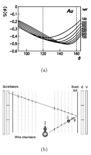
Figure 55: (a) Mott scattering analyzing power $S(\vartheta)$ for ¹⁹⁷Au obtained by interpolation of the Sherman tables SHER56 . (b) The principle of the experiment. The electrons are backscattered from the spin analyzer Au foil. From the electron tracks, the scattering angle and the Mott scattering asymmetry can be determined.

The principle of the measurement is sketched in Fig. 2b. The electron emitted from a polarized neutron and scattered from an analyzing foil is tracked by a system of two multiwire gas chambers and stops in the plastic scintillator. In this way, all the angular and energy information necessary to determine the momentum of the electron and the Mott scattering asymmetry is provided.

For the vertically oriented neutron spin in a simultaneous measurement of $R$ and $N$ one of the correlations will produce an up-down asymmetry while the other leads to a forward-backward asymmetry. Turning the neutron polarization by 90^∘ between the beam axis and the vertical axis interchanges the relation of the correlations to the observable asymmetries. One can now fully appreciate the measurement of $N$ as an aid for the $R$-measurement: because the deviation of $N$ from its SM-value is expected to be small (as implied by the good knowledge of the asymmetry parameters $A$ and $B$) it provides an ideal, positive-effect calibration of the apparatus.

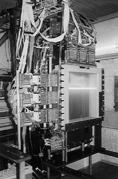
Figure 56: Full size MWPC-1 placed inside the experimental bunker. The neutron decay chamber is disassembled.

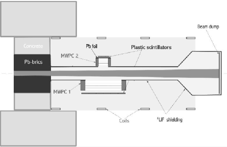
Figure 57: Layout of the experimental setup where the missing MWPC-2 has been replaced by the prototype detector. A 30 mg/cm² thick Pb foil is used as the Mott target.

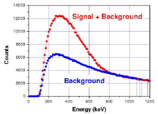
(a)

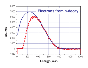
(b)

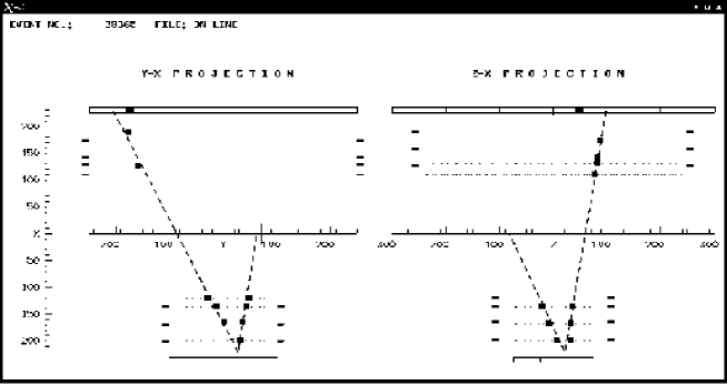
(c)

Figure 58: (a) Energy spectra of electrons reconstructed as coming from the neutron beam region (“Signal+Background”) and originating in walls (“Background”), respectively. (b) Experimental energy spectrum after background subtraction. The solid line represents the theoretical $\beta$ spectrum from neutron decay. (c) On-line display of a the Mott scattering event.

For fundamental physics experiments, a dedicated polarized cold neutron facility has been constructed at the spallation source SINQ. Its description can be found in Ref. NEUN00 . New measurements give the following performance parameters at the place of the experimental setup:

Flux:	($2.46\pm 0.04$)	$\times 10^{8}\;\textrm{(cm}^{2}\cdot\textrm{s}\cdot\textrm{mA)}^{-1}$
Equivalent thermal flux:	($6.49\pm 0.10$)	$\times 10^{8}\;\textrm{(cm}^{2}\cdot\textrm{s}\cdot\textrm{mA)}^{-1}$
Total intensity:	($1.48\pm 0.03$)	$\times 10^{10}\;\textrm{(s}\cdot\textrm{mA)}^{-1}$
Density:	($2.95\pm 0.04$)	$\times 10^{3}\;\textrm{(cm}^{3}\cdot\textrm{mA)}^{-1}$
Mean polarization:	($95.05\pm 0.09$)	%
Horizontal divergence:	0.014	rad
Vertical divergence:	0.011	rad

An efficient detector providing good rejection of undesired events is of primary importance. The key method of selecting the true events, where the electron emitted in the neutron decay was scattered from the analyzing foil, is based on the electron identification via energy spectrum and the reconstruction of the scattering vertex: the measured energy (corrected for losses) must not exceed the end-point energy of 783 keV and the reconstructed scattering vertex must be located on the analyzing foil.

These two conditions governed the laboratory development of prototype detectors and optimization studies for the experimental environment around the decay source: the part of the neutron beam viewed by detectors. The detector should have low mass and should be constructed of low Z materials. This leads to the concept of a gas detector with all electrodes of thin wire grids and gas mixture based on helium. Also the neutron beam must be transported in pure helium in front of the thin window (Mylar, 2 $\mu$m). The results of the laboratory investigations of the prototype MWPC are described in detail in Ref. BODE01 . The experience made by testing this detector in the real environment influenced by neutron beam led to a construction of the full size detectors with an active area of $50\times 50\;\textrm{cm}^{2}$. Now the first one of two MWPCs (see Fig. 3) is systematically investigated in the setup shown schematically in Fig. 4. The missing second MWPC has been replaced by the laboratory prototype. In this way, the trigger and the readout electronics can be reliably tested, too.

Sample data taken with the present setup are promising: the electrons originating from neutron decay are clearly identified as can be seen in Figs. 58(a) and 58(b). The missing part of the experimental $\beta$ spectrum at low energies is due to absorption effects in gas and the energy threshold of the scintillation detectors. Fig. 58(c) shows the on-line display of an example Mott scattering event.

It is planned that the experiment should start data taking in summer 2003 and within a few months should collect enough data for the anticipated accuracy of $5\times 10^{-3}$ for the $R$- and $N$-correlation parameters in the decay of free neutrons.

*The Measurement of Neutron Decay Parameters with the Spectrometer PERKEO II The Measurement of Neutron Decay Parameters
with the Spectrometer PERKEO II M.B. Kreuz^1,2 M.B. Kreuz

83 Introduction

Particle physics tries to examine structure and strength of particle interactions and particle properties. Traditionally, it is associated with high energy physics working in the energy range of presently $GeV$ and $TeV$. In contrast, our experiment was done with cold neutrons whose energies are even much lower than those of ordinary gas molecules at the other end of the energy spectrum.
In the Standard Model of elementary particle interactions the fundamental fermionic constituents of matter are leptons and quarks found in three generations. In the decay of free neutrons a d-quark couples to a u-quark and the electron to an electron-antineutrino via a W-Boson exchange. This is a simple process where all particles of the first family are present. It allows to derive precise information about the first generation of the Standard Model and to access a number of interesting questions in particle physics, for example

• the ratio of the coupling constants $\lambda=\frac{g_{A}}{g_{V}}$ (beta asymmetry $A$)

• the quark mixing and the unitarity of the CKM matrix ($A$ and neutron lifetime $\tau$)

• the universality of the electroweak interaction ($A$ and $\tau$)

• the origin of parity violation and the proposed existence of right handed currents (neutrino asymmetry $B$)

• a violation of time reversal invariance beyond the Standard Model (triple correlations D and R torsten )

In all these fields important progress has been made in the last few years.

84 The Spectrometer PERKEO

The spectrometer PERKEO II reich99 reich00 was build to access several of these coefficients, in particular the beta asymmetry $A$ and the neutrino asymmetry $B$, describing the correlation between the neutron spin and the momenta of the electron and the neutrino respectively. For $A$, it is sufficient to detect the decay electrons with respect to the neutron spin. For $B$ both the electron and the proton have to be traced to be able to deduce the neutrino direction.

We use the measurement scheme shown in Fig.59. A spin polarized, high flux cold neutron beam passes the spectrometer perpendicular to a strong magnetic field of 1T, created by large superconducting coils in a split pair configuration. Some of the neutrons will decay inside the spectrometer in the volume defined by a set of baffles. The uncharged neutrons pass the magnetic field without deviation, but the charged decay products – i.e. the electron and the proton – gyrate along the magnetic field lines and can be detected in the two detectors left and right of the beam. By using the magnetic field many problems of beta decay experiments are suppressed: the solid angle is well known to be $2\times 2\pi$. In addition the count rate is rather high because all particles reach the detector. By this the signal to background ratio improves accordingly.

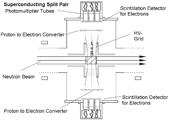
Figure 59: Layout of the spectrometer PERKEO for the measurement of the correlation $B$. The electron and the proton from the neutron decay are guided by a $1T$ magnetic field to the two combined electron proton detectors.

For the electron detection, plastic scintillators with photomultiplier readout are used. This is a fast and efficient combination. The threshold for electrons is 60keV. For the $A$ measurement count rates of about 300s^-1 have been obtained. In addition false effects from electron backscattering – a serious source of systematic error in beta spectroscopy – are suppressed by the magnetic field.

The detection of the protons is a challenge due to their low energy ($<750$eV). For systematic reasons we also wanted to be able to detect both particles in both hemispheres (see section 86). To this aim, the protons are converted into electrons via a negatively charged thin carbon foil: they are accelerated by the negative potential towards the foil where they create secondary electrons, which can be detected in the electron detector stratowa . Since the electric potential is considerably lower than the electron energies observable in the experiment, the electrons will pass the foils unhindered.

85 The Beta Asymmetry A

As already mentioned for the determination of the beta asymmetry $A$ only the electrons have to be detected. In our experiment, the experimental asymmetry in two detectors is defined by

$$A_{exp}:=\frac{N^{\uparrow\uparrow}-N^{\downarrow\uparrow}}{N^{\uparrow\uparrow}+N^{\downarrow\uparrow}}=APf\frac{v}{c}$$ (218)

with the polarization $P$, the spin flip efficiency $f$, the electron velocity $v$ and the count rates parallel and antiparallel to the neutron spin $N^{\uparrow\uparrow}$ and $N^{\downarrow\uparrow}$.

$A$ is very sensitive to the ratio of the axial vector to vector coupling strength $\lambda=\frac{g_{A}}{g_{V}}$ of the weak interaction. In the Standard Model $A$ and $\lambda$ are linked by a simple formula:

$$A=-2\frac{|\lambda|^{2}-Re(\lambda)}{1+3|\lambda|^{2}}$$ (219)

From our experiment we get $A=-0.1189(7)$ and $\lambda=-1.274(2)$. The main experimental errors in this experiment have been the statistical error ($0.45\%$) and the determination of the neutron spin polarization ($0.3\%$). Since the last measurement, important improvements in both fields have been made. First, the neutron flux at the new ballistic supermirror guide at the instrument PF1B at the ILL is a factor of $3$ higher compared with the previous experimental zone harry . Second, a new arrangement of two supermirror polarizers allows to achieve an unprecedented degree of polarization of more than $99.5\%$ and its determination at the $0.1\%$ level sascha .

From $\lambda$ and the neutron lifetime $\tau$ pdgkreuz $g_{A}$ and $g_{V}$ can be determined. They are important parameters for many problems in astrophysics, e.g. for primordial nucleosynthesis. Furthermore, they can be used to test the Standard Model: According to the conserved vector current hypothesis (CVC) the value of $C_{V}$ is not changed by QCD effects in the nuclear medium, which has been checked for many nuclei. On the other hand, $g_{A}$ depends on the nuclear medium and has to be measured. The value of $g_{V}$ can also be used to determine the first element $V_{ud}$ of the quark mixing matrix or CKM matrix via

$$V_{ud}=\frac{g_{V}}{G_{F}}$$ (220)

with the Fermi coupling constant $G_{F}$. Together with the particle data group values for $V_{us}$ and $V_{ub}$, the unitarity of the CKM matrix required by the Standard Model can be tested for the first row. In a unitary matrix the squared sum of all rows and columns has to be equal to one. For our value of $V_{ud}$ the test reads

$$|V_{ud}|^{2}+|V_{us}|^{2}+|V_{ub}|^{2}=0.9917(29)$$ (221)

which gives a $2.7$ sigma deviation from the expected value abele . The particle data group uses the world average $V_{ud}=0.9728(12)$ from neutron decay, leading to a unitarity gap of only $2.2$ sigma pdgkreuz . Using data from nuclear beta decay, one still finds a $2.3$ sigma deviation hardy from unity. New measurements are required to determine whether a discrepancy between reality and the Standard Model has been found.

86 The Neutrino Asymmetry B

It is necessary to detect both electron and proton to be able to trace the neutrino and to measure the neutrino asymmetry $B$. In our setup with a combined electron-proton detector on both sides there are two possibilities to define an observable asymmetry: electron and proton in the same or in opposite hemispheres. We can define the following asymmetries:

$$B_{exp,1}=\frac{N^{\uparrow\uparrow\uparrow}-N^{\downarrow\uparrow\uparrow}}{N^{\uparrow\uparrow\uparrow}+N^{\downarrow\uparrow\uparrow}}$$ (222)

$$B_{exp,2}=\frac{N^{\uparrow\uparrow\downarrow}-N^{\downarrow\uparrow\downarrow}}{N^{\uparrow\uparrow\downarrow}+N^{\downarrow\uparrow\downarrow}}$$ (223)

The arrows indicate the direction of the neutron spin and the hemisphere direction of the electron and proton respectively.

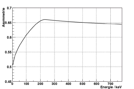
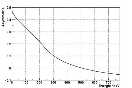
Figure 60: Electron-proton asymmetry in dependence of the electron energy for both possible configurations. Top: both particles in the same hemisphere. Bottom: in opposite hemispheres.

The resulting dependence of the asymmetry from the electron energy can be seen in Fig.60. From a systematic point of view it is much better to use the same hemisphere: If electron and proton are detected in the same detector the direction of the neutrino is well defined. Therefore the asymmetry is almost independent from the electron energy and thus insensitive to the detector calibration and resolution. In addition the influence of other asymmetry coefficients is suppressed and a high statistical sensitivity for $B$ is achieved over the complete energy range. In the case of opposite hemispheres the direction of the neutrino is not well defined and the asymmetry depends strongly on the electron energy. Furthermore, the result depends on a precise knowledge of the beta asymmetry parameter $A$ and the The highest sensitivity to $B$ is in the low energy part of the spectrum where the spectroscopy is most difficult because of background and threshold effects. Considering these systematics an evaluation of the asymmetry of equation222 is strongly preferable, but any measurement with PERKEO will automatically allow both.

In contrast to $A$, $B$ is not very sensitive to the ratio of the coupling strengths $\lambda$. But since $B$ measures directly the antineutrino asymmetry, it is rather sensitive to a hypothetical admixture of right handed components to the weak interaction which is purely left handed in the Standard Model. It can be used to test left right symmetric models. In these models parity is not violated for high energies and even in our low energy world it should not be maximally violated. Small remnants of the right handed currents can still be found, suppressed by the much higher mass of the corresponding W-Boson. The manifest left right symmetric models are described by three parameters: the mixing angle $\zeta$ between the weak W-eigenstates and the mass eigenstates, the ratio $\delta$ of the square of the boson masses and the ratio $\lambda$ of the coupling constants. Using $A$ and $B$ from the experiment and $\tau$ from the PDG an exclusion plot in the $\delta-\zeta$-plane can be drawn. The Standard Model ($\delta=0$, $\zeta=0$) lies within the allowed region at $90\%$ confidence level. Please note that these are not the best limits reached so far by high energy physics and astronomy, but due to the high sensitivity of B, a slight improvement of the precision will make them competitive. The evaluation of our 2001 measurement of the neutrino asymmetry is still in progress. It should be finished at the end of 2003.

87 Summary

Within our group two different correlation coefficients in the decay of free neutrons have been measured and precision tests of the Standard Model have been performed. $V_{ud}$ the first element of the CKM matrix has been derived from neutron decay experiments in such a way that a unitarity test of the CKM matrix can be performed based solely on particle physics data. With this value we find a 2.7 sigma deviation from unitarity.

*Summary Talk Summary Talk N. Severijns

88 Unitarity

At the current level of precision the unitarity test based on the first row of the CKM quark mixing matrix depends only on the $V_{ud}$ and $V_{us}$ matrix elements.

The $V_{ud}$ matrix element is determined in beta decay processes. At their respective precisions the results from the superallowed $0^{+}\rightarrow 0^{+}$ pure Fermi transitions (i.e. $V_{ud}$ = 0.9740(5) hardy02 ), from the lifetime $\tau$ and the electron asymmetry parameter $A$ in neutron decay (i.e. $V_{ud}$ = 0.9740(13)abele02 ) and from the pion beta decay branch (i.e. $V_{ud}$ = 0.9771(56) pocanic02 ) agree with each other and point to a 2 $\sigma$ to 2.5 $\sigma$ deviation from unitarity.

The highest precision at present is reached by the superallowed $0^{+}\rightarrow 0^{+}$ transitions. The error bar is in this case dominated by the corrections. Although theorists believe that both the radiative as well as the nuclear structure related corrections are well under control, the isospin corrections are rather frequently questioned. At several facilities experimental programs are therefore ongoing to acquire experimental information that should allow one to check the reliability of these corrections.

Due to important recent progress in the experimental precision for both the lifetime $\tau$ and the electron asymmetry parameter $A$ in neutron decay the precision of the $V_{ud}$ value from neutron decay is now almost at the same level of precision as the one from the $0^{+}\rightarrow 0^{+}$ transitions. A number of new measurements is moreover being prepared or well advanced already. In addition, important cross checks will be provided by new measurements of the electron-neutrino correlation coefficient $a$ (with about an order of magnitude higher precision) as well as by a combined measurement of the electron asymmetry parameter $A$, the neutrino asymmetry parameter $B$ and the electron-neutrino correlation coefficient $a$ in neutron decay.

In pion decay, reaching a high precision for $V_{ud}$ is hampered by the low beta decay branching ratio of order $10^{-8}$ only. However, the analysis of a currently available large data set from a recent experiment at PSI will significantly improve the value mentioned above. It is finally important to note that the error on the $V_{ud}$ values obtained from neutron decay and from pion beta decay are still dominated by the experimental error bars. New measurements that allow one to further reduce these should therefore be strongly supported.

The $V_{us}$ matrix element is determined most precisely in Kaon decay. As it turns out, the presently accepted value for $V_{us}$ is based on experiments that were carried out about 25 years ago. Recent results obtained in $K_{e3}$ decay at Brookhaven indicate that the branching ratios on which the value for $V_{us}$ is based may be off by several standard deviations. If so, it is not excluded that this might solve the unitarity problem. New efforts that are being planned in this respect renk ; delucia should clarify this.

It is interesting to note that measurements planned at the CLEO-c facility that is constructed to do charm physics at threshold, which in general yields clean signals, will soon allow one to test unitarity also for other rows and columns of the CKM matrix. Most important will be the determination of the $V_{cd}$ matrix element with an anticipated precision of about 1.7% shipsey , which would yield a unitarity test for the first column with an almost identical precision to that obtained now for the first row. This will indicate whether the current deviation from unitarity for the first row is more likely to be due to a problem with $V_{ud}$ or with $V_{us}$. In addition, the determination of the $V_{cs}$ matrix element with an about 1.6% precision shipsey would allow to test unitarity also for the second row and the second column, although with somewhat less precision.

89 Search for new weak interactions

Apart from providing important input information to test unitarity, correlation experiments in neutron decay also provide very important tests for the presence of scalar, tensor or right-handed weak interactions that are not included in the Standard Model and would be mediated by gauge bosons other than the W- and Z-bosons or by leptoquarks. The potential of neutron decay experiments in this respect was demonstrated several years ago already by Mostovoi et al. mostovoi00 , and this type of physics interpretation of correlations in neutron decay will certainly gain in importance as the experimental precision increases further. At that point it will also become important to include in the analysis of the data the Fierz interference term $b$ (which is zero in the Standard Model) as well as radiative and recoil corrections, which are now usually neglected. Measurements of the energy dependence of the recoil corrections to the electron asymmetry parameter $A$ and the electron-neutrino correlation coefficient $a$ would lead to improved CVC and second class current tests.

90 Time reversal violation

In recent years a lot of progress was made in searches for the neutron electric dipole moment. The current limit for the neutron EDM has ruled out already a number of models and is close to the discovery limit for other models. Large efforts are currently ongoing at several places to further improve on this, mainly based on the design of powerful ultra cold neutron facilities. With the planned and ongoing developments of new UCN sources that will provide unprecedented amounts of neutrons, an improvement of two orders of magnitude seems realistic, thereby improving the sensitivity for neutron EDM experiments to about 2 x $10^{-28}$ e cm. These efforts should be strongly supported.

Other ongoing searches for T-violation in neutron decay, i.e. determinations of the D- and R-triple correlation coefficients, should be pursued as well as these can be interpreted with much fewer theoretical uncertainties than the EDM, or they are complementary.

91 Technical advances

Recent new ideas for alternative measurement principles and new set-ups for lifetime and correlation measurements with both cold and ultra cold neutrons have already lead and will still lead to reduced systematic errors and increased statistics. Especially important in this respect are the successful new developments with respect to neutron polarimetry. Using supermirrors a precision of 0.5% is now routinely available, while polarized ${}^{3}He$ polarimeters even allow one to limit the uncertainty on the neutron polarization to as low as 0.1%. Further, several facilities providing cold and ultra cold neutrons will provide both higher intensity beams as well as pulsed beams, thereby allowing for significant experimental improvements.

92 Conclusion

The field of fundamental research in neutron decay is very active. In the past decade significant progress was made with respect to the obtainable experimental precision, both due to increased neutron beam intensities and the development of improved neutron polarimetry techniques. With the presently ongoing technical developments, the large amount of new ideas for improved experimental set-ups, and the new approaches for the determination of several observables in neutron decay that are currently available and being developed, the neutron will also in the next decade remain an important laboratory for fundamental weak interaction physics.

*List of Participants

List of Participants

References

- (1) M. Kobayashi and T. Maskawa, Prog. Theor. Phys. 49 (1973) 652.
- (2) N. Cabibbo, Phys. Rev. Lett. 10 (1963) 531.
- (3) L.-L. Chau and W.-Y. Keung, Phys. Rev. Lett. 53 (1984) 1802; H. Harari and M Leurer, Phys. Lett. B181 (1986) 123; H. Fritzsch and J. Plankl, Phys. Rev. D35 (1987) 1732 ; F. J. Botella and L.-L. Chao, Phys. Lett. B168 (1986) 97.
- (4) L. Wolfenstein, Phys. Rev. Lett. 51 (1983) 1945 (1983).
- (5) K. Hagiwara et al., Phys. Rev. D66 (2002) 10001
- (6) J. C. Hardy and I. S. Towner, talk at WEIN98, Santa Fe, June 14-21, 1998 and nucl-th/9809087.
- (7) Yu. A. Mostovoi et al., Phys. Atomic Nucl. 64, 1955 (2001); P. Liaud, Nucl. Phys. A612 (1997) 53. H. Abele et al., submitted to Phys. Rev. Lett. 2001, as a final result of J. Reich et al., Nucl. Instr. Meth. A440 (2000) 535
- (8) H. Leutwyler and M. Roos, Z. Phys. C25, 91 (1984). See also the work of R. E. Shrock and L.-L. Wang, Phys. Rev. Lett. 41, 1692 (1978). V. Cirigliano et al., Eur. Phys. J. C23, 121 (2002). G. Calderon and G. Lopez Castro , Phys. Rev. D65, 073032 (2002).
- (9) H. Abramowicz et al., Z. Phys. C15, 19 (1982). S. A. Rabinowitz et al., Phys. Rev. Lett. 70, 134 (1993); A. O. Bazarko et al., Z. Phys. C65, 189 (1995). N. Ushida et al., Phys. Lett. B206, 375 (1988).
- (10) The LEP Collaborations, the LEP Electroweak Working Group and the SLD Heavy Flavour and Electroweak Groups, hep-ex/0112021v2, 2002.
- (11) M. Artuso and E. Barbieri, Mini-Review of in the 2002 Review of Particle Physics.
- (12) M. Battaglia and L. Gibbons, mini-review of in the 2002 Review of Particle Physics.
- (13) T. Affolder et al., Phys. Rev. Lett. 86, 3233 (2001).
- (14) O. Schneider, mini-review on - mixing in the 2002 Review of Particle Physics.
- (15) The relevant QCD corrections in leading order in F. J. Gilman and M. B. Wise Phys. Lett. B93, 129 (1980) and Phys. Rev. D27, 1128 (1983), have been extended to next-to-leading-order by A. Buras et al., Ref. 39; S. Herrlich and U. Nierste Nucl. Phys. B419, 292 (1992) and Nucl. Phys. B476, 27 (1996).
- (16) The limiting curves in Figure 2 arising from the value of correspond to values of the hadronic matrix element expressed in terms of the renormalization group invariant parameter from 0.75 to 1.10 . See, for example, L. Lellouch, plenary talk at Lattice 2000, Bangalore, India, August 17 - 22, 2000, in Nucl. Phys. Proc. Suppl. 94, 142 (2001).
- (17) B. Aubert et al., SLAC preprint SLAC-PUB-9153, 2002 and hep-ex/0203007.
- (18) K. Abe et al. (Belle Collaboration), Belle Preprint 2002-6 and hep-ex/0202027v2, 2002.
- (19) H. Burkhardt et al., Phys. Lett. B206 (1988) 169.
- (20) G. D. Barr et al., Phys. Lett. B317 (1993) 233 ; L. K. Gibbons et al., Phys. Rev. Lett. 70 (1993) 1203; V. Fanti et al.,Phys. Lett. B465 (1999) 335; A. Alavi-Harati et al., Phys. Rev. Lett. 83 (1999) 22; A. Lai et al. Europhys. Lett. C22 (2001) 231.
- (21) L.-L. Chau and W. Y. Keung, Ref. 3; J. D. Bjorken, private communication and Phys. Rev. D39 (1989) 1396 (1989); C. Jarlskog and R. Stora, Phys. Lett. B208 (1988) 268; J. L. Rosner, A. I. Sanda, and M. P. Schmidt, in Proceedings of the Workshop on High Sensitivity Beauty Physics at Fermilab, Fermilab, November 11 - 14, 1987, edited by A. J. Slaughter, N. Lockyer, and M. Schmidt (Fermilab, Batavia, 1988), p. 165; C. Hamzaoui, J. L. Rosner, and A. I. Sanda, ibid., p. 215.
- (22) C. Jarlskog, Phys. Rev. Lett. 55 (1985) 1039 and Z.Phys. C29 (1985) 491.

References

- (1) I.S. Towner and J.C. Hardy, Proc. of the V Int. WEIN Symposium: Physics Beyond the Standard Model, Santa Fe, NM, June 1998, edited by P. Herczeg, C.M. Hoffman and H.V. Klapdor-Kleingrothaus (World Scientific, Singapore, 1999) pp. 338-359.
- (2) J.C. Hardy, I.S. Towner, V.T. Koslowsky, E. Hagberg and H. Schmeing, Nucl. Phys A509, 429 (1990).
- (3) K. Hagiwara et al , Phys. Rev. D 66, 010001 (2002).
- (4) H. Abele, M.A. Hoffmann, S. Baessler, D. Dubbers, F. Gluck, U. Muller, V. Nesvizhevsky, J. Reich and O. Zimmer, Phys. Rev. Lett. 88, 211801 (2002).
- (5) I.S. Towner and J.C. Hardy, Phys. Rev. C 66, 035501 (2002).
- (6) J.C. Hardy and I.S. Towner, Phys. Rev. Lett. 88, 252501 (2002).
- (7) J.C. Hardy et al, to be published.

References

- (1) A. Sirlin, Phys. Rev. 164, 1767 (1967).
- (2) I. Towner and J. Hardy, Phys. Rev. C66, 035501 (2002).
- (3) W. Jaus and G. Rasche, Nucl. Phys. A143, 202 (1970); Phys. Rev. D35, 3420 (1987); A. Sirlin and R. Zucchini, Phys. Rev. Lett. 57, 1994 (1986); A. Sirlin, Phys. Rev. D35, 3423 (1987).
- (4) A. Czarnecki, W. Marciano and A. Sirlin, prepint in preparation.
- (5) A. Sirlin, Rev. Mod. Phys. 50, 573 (1978).
- (6) W. Marciano and A. Sirlin, Phys. Rev. Lett. 56, 22 (1986).
- (7) A. Sirlin, in Precision Tests of the Standard Electroweak Model (ed. P. Langacker, World Sci. 1995) p. 776.

References

- (1) Particle Data Group, Phys.Rev.D 66 (2002) 01001
- (2) D.N.Schramm, Proc. 25th Int. Conf. on High Energy Physics, eds K.K.Phua and Y.Yamaguchi, Singapore (1991)1311
- (3) J.N.Bahcall et al., Rev.Mod.Phys. 54 (1982)767; 60 (1988) 296
- (4) I.S.Towner and J.C.Hardy, Physics Beyond the Standard Model, eds. Herczeg et al. World Scientific (1998) 322
- (5) J.F.Donoghue et al., Dynamics of the Standard Model, Cambridge (1992) 63
- (6) B.R.Holstein, Rev. Mod. Phys. 46 (1974) 789
- (7) J.D.Jackson et al., Phys. Rev. 106 (1957) 107
- (8) A.Garcia, JETP Lett. 27 (1978) 510
- (9) A.S.Carnoy et al., Phys.Rev.D 38 (1988) 1636; J.Phys.G 18 (1992) 823
- (10) J.Deutsch and P.Quin, Precision Tests of the Standard Model, ed.P.Langacker, World Scientific (1995) 706
- (11) O. Nachtmann, Zeits.Phys. 215 (1968) 505
- (12) H.Abele, Nucl.Instr.and Meth.in Phys.Res.A 440 (2000) 499
- (13) A.P.Serebrov et al., JETP 86 (1998)1074
- (14) Yu A.Mostovoi et al. Physics of Atomic Nuclei 64 (2001) 1955
- (15) S.Weinberg, Phys. Rev. 115 (1959) 481
- (16) F.Glück, Phys.Lett. B 376 (1996) 25
- (17) J.Byrne, Europhys.Lett. 56 (2001) 633
- (18) M.Beck et al., Pis’ma v ZhETF 76 (2002) 392

References

- (1) S. Arzumanov, L. Bondarenko, S. Chernyavsky, W. Drexel, A. Fomin, P. Geltenbort, V. Morozov, Yu. Panin, J. Pendlebury, K. Schreckenbach, Phys. Lett. B 483 (2000) 15.
- (2) W.Mampe , P.Ageron ,C.Bates, J.M. Pendlebury and A. Steyerl, Phys. Rev. Lett. 63 (1989) 593.
- (3) V.Nesvizhevskii, A. Serebrov, et al. , Sov.JETP 75 (1992) 405.
- (4) W. Mampe, L. Bondarenko, V. Morosov, et al. JETP Lett. 57 (1993) 82.
- (5) H. Abele et al., Physics Letters B 407 (1997) 212.
- (6) K.Schreckenbach, P.Liaud et al.,Phys.Lett. B349 (1995) 427.
- (7) B.Erozolimskii, I.Kuznetsov et al., Phys.Lett. B263 (1991) 33.
- (8) D.Dubbers, W.Mampe and J. Dorner, Europhys. Lett. 11 (1990) 195.
- (9) K. Schreckenbach and W. Mampe, J.Phys. G 18 (1992) 1.
- (10) V.Morozov, Storing of ultracold neutrons in closed vessels, review. Goskomatom USSR, NIIAtomReactors, Dimitrovgrad, 1982.
- (11) V. Nesvizhevsky et al., ILL Annual Report 1997, p.62; JINR Commun, P3-98-79, Dubna, 1998.
- (12) L.Bondarenko, E.Korobkina, V.Morozov et al. ILL Experimental Report no.3-14-44 (1997); JETP Lett., v.68, iss.9, p.691, 1998, see also 6th International Seminar on Interaction of Neutrons with Nuclei, Dubna, May 1998, p.101.
- (13) Yu. Mostovoi. Preprint RRC Kurchatov Institute IAE-6040/2, 1997.
- (14) C.Caso et al. (PDG), European Phys.Jour. C3, 1(1998); URL: http://pdg.lbl.gov p.2.

References

- (1) K. Hagiwara et al., Phys. Rev. D 66 010001 (2002).
- (2) W.J. Marciano and A. Sirlin, Phys. Rev. Lett. 56 (1986) 22.
- (3) P. Langacker and D. London, Phys. Rev. D 38 (1988) 886.
- (4) J. Maalampi and M. Roos, Phys. Rep. 186 (1990) 53.
- (5) P. Langacker and M. Luo, Phys. Rev. D 45 (1992) 278.
- (6) W.J. Marciano and A. Sirlin, Phys. Rev. D 35 (1987) 1672.
- (7) J. Deutsch in Workshop on the breaking of fundamental symmetries in nuclei, Santa Fe, 1988: B.R. Holstein and S. B. Treiman, Phys. Rev. D 16 (1977) 2369.
- (8) Y. Liao, X. Li, Phys. Lett. B 503 (2001) 301.
- (9) J. Hardy et al., nucl-th/9812036 (1998).
- (10) D. Pocanic, PIBETA : a precise measurement of the pion -decay rate to determine , ref. HADM .
- (11) M Battaglia, AJ Buras, P Gambino and A Stocchi, eds. Proceedings of the First Workshop on the CKM Unitarity Triangle, CERN, Feb 2002, hep-ph/0304132.
- (12) W. Marciano, New Analysis of Neutron -Decay (Radiative Corrections) and Implications for CKM Unitarity”, ref. HADM .
- (13) D.H. Wilkinson, Nucl. Phys. A 377 (1982) 474; S. M. Bilenkii et al., Soviet. Phys. JETP 37 (1960) 1241.
- (14) F. Glück and K. To’th, Phys. Rev. D 46 (1992) 2090; R. T. Shann, Nuovo Cimento A5 (1971) 591.
- (15) H. Abele et al., Phys. Rev. Lett. 88 211801 (2002).
- (16) I.S. Towner, Nucl. Phys. A 540 (1992) 478; J. Hardy et al., nucl-th/9812036 (1998).
- (17) H. Abele et al., Phys. Lett. B 407 (1997) 212.
- (18) J. Reich et al., Nucl Instr. & Meth. A 440 (2000) 535.
- (19) C.Sbarra, talk at the Rencontre de Moriond, Les Arcs, Savoie, France (March 11-18, 2000).
- (20) P. Bopp et al., Phys. Rev. Lett. 56 (1988) 919.
- (21) B.G. Yerozolimsky et al. Phys. Lett. B 412 (1997) 240; B.G. Erozolimskii et al., Phys. Lett. B 263 (1991) 33.
- (22) K. Schreckenbach et al., Phys. Lett. B 349 (1995) 427; P. Liaud et al., Nucl. Phys. A 612 (1997) 53.
- (23) H. Haese et al., Nucl. Instrum. Methods Phys. Res. A485, 453, 11.06.2002.
- (24) T. Soldner, Recent progress in neutron polarization and its analysis, ref. HADM .
- (25) W. Heil et al., Physica B 241 (1998) 56.
- (26) O. Zimmer et al., Nucl. Instr. & Meth. A 440 764 (2000).
- (27) D. Dubbers, Correlation measurements in pulsed beams, ref. HADM .
- (28) H. Abele, D. Mund, eds. these proceedings, workshop of Quark-Mixing, CKM-Unitarity.

References

-
(1)
N. Cabibbo, Phys. Rev. Let. 10 (1963) 531;
M. Kobayashi and T. Maskawa, Prog. Theor. Phys. 49 (1973) 652. - (2) D.E. Groom et al., Phys. Rev. D66 (2002) 1.
- (3) ALEPH Collaboration, R. Barate et al., Phys. Lett. B465 (1999) 349.
- (4) DELPHI Collaboration, P. Abreu et al., Phys. Lett. B439 (1998) 209.
- (5) OPAL Collaboration, G. Abbiendiet al., Phys. Lett. B490 (2000) 71.
-
(6)
’LEP W Mass and Width combinations’,
http://lepewwg.web.cern.ch/LEPEWWG/lepww/mw/ - (7) http://lepewwg.web.cern.ch/LEPEWWG/lepww/4f/ and references therein.
- (8) W. Beenakker et al., “WW Cross-Sections and Distributions”, in “Physics at LEP2”, eds. G. Altarelli et al., CERN 96-01
- (9) DELPHI Collaboration, P. Abreu et al., Phys.Lett.B439 (1998) 209.
- (10) J.Letts and P.Mattig Eur.Phys.J.C21 (2001) 211.

References

- (1) http://pibeta.phys.virginia.edu/ or http://pibeta.web.psi.ch.
- (2) W Jaus, Phys. Rev. D 63, 053009 (2001).
- (3) V Cirigliano, M Knecht, H Neufeld and H Pichl, hep-ph/0209226.
- (4) W K McFarlane, et al., Phys. Rev. D 32, 547 (1985).
- (5) F J Gilman, et al., in “Review of Particle Physics”, Phys. Rev. D 66, 01001-113 (2002).
- (6) W J Marciano and A. Sirlin, Phys. Rev. Lett. 56, 22 (1986).
- (7) V N Bolotov et al., Phys. Lett. B 243, 308 (1990).
- (8) V N Bolotov et al., Sov. J. Nucl. Phys. 51, 455 (1990).
- (9) A A Poblaguev, Phys. Lett. B 238, 108 (1990).
- (10) A A Poblaguev, Phys. Lett. B 286, 169 (1992).
- (11) P Herczeg, Phys. Rev. D 49, 247 (1994).

References

- (1) The Particle Data Group, Phys. Rev. D66, Part I, 113 (2002)
- (2) H. Leutwyler and M. Roos, Z. Phys. C25, 91 (1984)
- (3) M. Bourquin et al., Z. Phys. C12, 307 (1982)
- (4) M. Bourquin et al., Z. Phys. C21, 1 (1983)
- (5) M. Bourquin et al., Z. Phys. C21, 17 (1983)
- (6) J. Wise et al., Phys. Lett. B91, 165 (1980)
- (7) S.Y. Hsueh et al., Phys. Rev. D38, 2056 (1988)
-
(8)
A. Alavi-Harati, Phys. Rev. Lett. 87, 132001 (2001)
N. Solomey, hep-ex/0010073 (2000) - (9) R. Flores-Mendieta, E. Jenkins and A.V. Manohar, UCSD/PTH 98-17 and hep-ph/9805416 (1998)
- (10) J. Anderson and M.A. Luty, Phys. Rev. D47, 4975 (1993)
- (11) J. Donoghue, B. Holstein and W. Klimt, Phys. Rev. D35, 934 (1987)
- (12) A. Krause, Helv. Phys. Acta 63, 3 (1990)
- (13) F. Schlumpf, Phys. Rev. D51, 2262 (1995)
- (14) K. Toth, K. Szego, T. Margaritisz, Phys. Rev. D33, 3306 (1986)
- (15) F. Glück, I. Joó, Phys. Lett. B340, 240 (1994)

References

- (1) V. Grigoryev, A. Grishin, V. Vladimirsky, et al Sov. J. Nucl. Phys 6, 329 (1967)
- (2) C. Stratova, R. Dobrozemskii, V. Weinzierl, et al Phys. Rev. (D18), 3970 (1978)
- (3) J. Byrne, P. G. Dawber, M. G. D. van der Grinten, et al Journal of Physics G: Nuclear and Particle Physics 28, 1325 (2002)
- (4) S. Balashov, Yu. Mostovoy Russian Research Center “Kurchatov Institute” Preprint IAE – 5718/2, Moscow (1995)

References

- (1)
- (2) Particle Data Group, K. Hagiwara et al., Phys. Rev. D 66, 010001 (2002)
- (3) J. Hardy, this proceedings
- (4) H. Abele et al., Phys. Rev. Lett. 88, 211801 (2002), and this proceedings
- (5) D. Dubbers et al., this proceedings
- (6) A. Young, this proceedings
- (7) Chr. Stratowa et al., Phys. Rev. D18, 3970 (1978)
- (8) J. Byrne et al., J. Phys. G 28, 1325 (2002), and this proceedings
- (9) O. Zimmer et al., Nucl. Inst. Meth. A440 (2000) 548, S. Baeßler et al., in preparation

References

- (1) H. Abele et al., Phys. Rev. Lett. 88 211801 (2002).
- (2) H. Haese et al., Nucl. Instrum. Methods Phys. Res. A485, 453, 11.06.2002.
- (3) T. Soldner, Recent progress in neutron polarization and its analysis. In: these proceedings, workshop of Quark-Mixing, CKM-Unitarity.

References

- (1) The members of the TRIP group at KVI are at present: G.P. Berg, U. Dammalapati, P. Dendooven, O. Dermois, M.N. Harakeh, R. Hoekstra, K. Jungmann, R. Morgenstern, A. Rogachevskiy, M. Sanchez-Vega, R. Timmermans, E. Traykov, L. Willmann, H.W. Wilschut
- (2) K. Jungmann, Acta Physica Polonica, 33, 2049 (2002)
- (3) J.W. Turkstra, Hyperf.Int. 127, 533 (2000); see also: “Trapped Radioactive Isotopes: -laboratories for fundamental Physics – TRIP ”, H.W. Wilschut et al., Aanvraag in het kader van het investeringsprogramma NWO-Groot (1999);
- (4) “Precision Tests of the Standard Electroweak Model”, P. Langacker (ed.) World Scientific, Singapore (1995)
- (5) M. Leino. Nucl. Instr. Meas. 126, 320 (1997)
- (6) “Atomic Physics at Accelerators: Laser Spectroscopy and Applications”, Hyperf.Int. 127, L. Schweikhard and H.-J. Kluge (eds.)
- (7) P. Herczeg, Prog. Part. and Nucl. Phys. 46, 413 (2001)
- (8) S.J.M. Kuppens et al., Phys.Rev. A 65, 023410 (2002)
- (9) J.W. Turkstra et al., Phys.Rev.Lett. 87, 123202 (2001)
- (10) “CP Violation without Strangeness”, I.B. Khriplovich, S.K. Lamoreaux, Springer, Berlin (1997)
- (11) M. Trodden, Rev.Mod.Phys. 71, 1463 (1999); A.D. Sakharov, A. D., JETP Lett. 5, 24 (1967)
- (12) N. Ramsey, at ”Breit Symposium”, Yale (1999)
- (13) C. Regan et al.,Phys.Rev.Lett.88, 071805 (2002); see also: E.A. Hinds and B.E. Sauer, Physics World 10, 37 (1997)
- (14) J. Bailey et al., Nucl. Phys. B150, 1 (1978)
- (15) M. Aciari, et al., Phys.Lett. B bf , (1998)
- (16) D. Cho et al. Phys.Rev.Lett. 63, 2559 (1989); see also: H.M. Quiney et al., Phys.Rev. A 57, 920 (1998)
- (17) P.G. Harris et al., Phys.Rev.Lett. 82, 904 (1999)
- (18) M.V. Romalis et al. Phys. Rev. Lett. 86, 2505 (2001)
- (19) P.G.H. Sandars, Contemp.Phys. 42, 97 (2001)
- (20) V. Dzuba et al., Phys.Rev. A 63, 062101 (2001)
- (21) W.C. Haxton and C.E. Wieman, Ann Rev.Nucl.Part.Sci. 51 261 (2001)
- (22) D. Fick, Hyperf.Int. 127, 463 (2000)

References

- (1) J. M. Doyle and S. K. Lamoreaux, Europhys. Lett. 26, (1994) 253.
-
(2)
C. E. H. Mattoni.
Magnetic Trapping of Ultracold Neutrons Produced Using
a Monochromatic Cold Neutron Beam.
PhD thesis, Harvard University, 2002.
Available at
http://www.doylegroup.harvard.edu/neutron/publications/publications.html. -
(3)
D. N. McKinsey.
Detecting Magnetically Trapped Neutrons: Liquid Helium As A
Scintillator.
PhD thesis, Harvard University, 2002.
Available at
http://www.doylegroup.harvard.edu/neutron/publications/publications.html. - (4) P. R. Huffman, C. R. Brome, J. S. Butterworth, K. J. Coakley, M. S. Dewey, S. N. Dzhosyuk, R. Golub, G. L. Greene, K. Habicht, S. K. Lamoreaux, C. E. H. Mattoni, D. N. McKinsey, F. E. Wietfeldt, and J. M. Doyle. Magnetic trapping of neutrons. Nature 403, 62–64 (2000).
-
(5)
C. R. Brome.
Magnetic Trapping of Ultracold Neutrons.
PhD thesis, Harvard University, 2000.
Available at
http://www.doylegroup.harvard.edu/neutron/publications/publications.html. - (6) R. Golub, D. Richardson, and S. K. Lamoreaux. Ultra-Cold Neutrons. Adam Hilger, 1991.
- (7) W. M. Burton and B. A. Powell. Fluorescence of tetraphenyl-butadiene in the vacuum ultraviolet. Applied Optics 12, 87–89 (1973).

References

- (1) J. Byrne, et al., Nucl. Instrum. Meth. A 284, 116 (1989); J. Byrne, et al., Phys. Rev. Lett. 65, 289 (1990); A. P. Williams, Ph.D. thesis, University of Sussex (unpublished, 1989); W. M. Snow, et al., Nucl. Instrum. Meth. A 440, 528 (2000);
- (2) J. Pauwels, et al., Nucl. Instrum. Meth. A 303, 133 (1991); R. D. Scott, et al., Nucl. Instrum. Meth. A 314, 163 (1992); J. Pauwels, et al., Nucl. Instrum. Meth. A 362, 104 (1995); R. D. Scott, et al., Nucl. Instrum. Meth. A 362, 151 (1995); Private communication, J. Pauwels fax to D. Gilliam and R. D. Scott, 17 Dec. 1993, Reg. No. 2367/93.
- (3) J. F. Ziegler, Stopping and Range of Ions in Matter (SRIM-2000).
- (4) A. D.Carlson, et al. The ENDF/B-VI Neutron Cross Section Measurement Standards, NISTIR 5177 (1993). Available from NTIS (http://www.ntis.gov/).
- (5) J. M. Richardson, W. M. Snow, Z. Chowdhuri, and G. L. Greene, IEEE Trans. Nucl. Sci. 45,550 (1998); Z. Chowdhuri et al., to be published in in Rev. Sci. Instr. (2003).

References

- (1) H. Abele, Nucl. Instr. Methods A 440, 499 (2000).
- (2) W. Paul, in Proc. Int. Conf. on Nuclear Physics and Physics of Fundamental Particles, Chicago, 1951.
- (3) W. Paul, F. Anton, L. Paul, S. Paul, W. Mampe, Z. Phys. C 45, 25 (1989).
- (4) W. Mampe, et al., Phys. Rev. Lett. 63, 593 (1989).
- (5) V.V. Nesvizhevskii et al.., Sov. Phys. JETP 75, 405 (1992).
- (6) W. Mampe et al., JETP Letters 57, 82 (1993).
- (7) J. Byrne et al., Europhys. Lett. 33, 187 (1996).
- (8) S.S. Arzumanovet al., Nucl. Instr. Methods A 440, 511 (2000).
- (9) A. Pichelmaier et al., Nucl. Instr. Methods A 440, 517 (2000).
- (10) K. Hagiwara et al. (Particle Data Group), Phys. Rev D 66, 110001 (2002).
- (11) V.V. Vladimirskii, Sov. Phys. JETP 12,740 (1961)
- (12) G. Petzoldt, Diploma thesis, Technische Universität München, 2001 (unpublished); G. Petzoldt et al., to be published.

References

- (1) O. Schärpf and N. Stüsser: NIM A 284 (1989) 208.
- (2) O. Schärpf: Physica B 156/157 (1989) 639.
- (3) O. Zimmer: Phys. Lett. B 461 (1999) 307.
- (4) O. Zimmer, T.M. Müller, P. Hautle, W. Heil, and H. Humblot: Phys. Lett. B 455 (1999) 62.

References

- (1) F. Bloch and A. Nordsieck, Phys. Rev. 52 (1937) 54.
- (2) D. A. Bryman, P. Depommier and C. Leroy, Phys. Reports 88 (1982) 151.
- (3) H. F. Schopper, Weak Interactions and Nuclear Beta Decay (1966).
- (4) F. E. Low, Phys. Rev. 110 (1958) 974.
- (5) S. L. Adler and Y. Dothan, Phys. Rev. 151 (1966) 1267.
- (6) T. H. Burnett and N. M. Kroll, Phys. Rev. Lett. 20 (1968) 86.
- (7) H. W. Fearing, E. Fischbach and J. Smith, Phys. Rev. Lett. 24 (1970) 189; Phys. Rev. D 2 (1970) 542.
- (8) F. Glück and I. Joó, Comp. Phys. Comm. 107 (1997) 92.
- (9) F. Glück and I. Joó, Comp. Phys. Comm. 95 (1996) 111.
- (10) F. Glück, Comp. Phys. Comm. 101 (1997) 223.
- (11) F. Glück and K. Tóth, Phys. Rev. D 41 (1990) 2160.
- (12) F. Glück and K. Tóth, Phys. Rev. D 46 (1992) 2090.
- (13) Y. Yokoo and M. Morita, Suppl. Prog. Theor. Phys. No. 60 (1976) 37.
- (14) A. Garcia and M. Maya, Phys. Rev. D 17 (1978) 1376.
- (15) K. Tóth, KFKI-1984-52.
- (16) K. Tóth, K. Szegő and A. Margaritis, Phys. Rev. D 33 (1986) 3306.
- (17) K. Tóth and F. Glück, Phys. Rev. D 40 (1989) 119.
- (18) S. Y. Lee, Phys. Rev. D6 (1972) 1803; R. N. Mohapatra and S. Sakakibara, Phys. Rev. D9 (1974) 429; W. Angerson, Nucl. Phys. B69 (1974) 493.
- (19) A. Sirlin, Nucl. Phys. B71 (1974) 29; Phys. Rev. Lett. 32 (1974) 966; Nucl. Phys. B100 (1975) 291.
- (20) A. Sirlin, Rev. Mod. Phys. 50 (1978) 573.
- (21) A. Sirlin, Phys. Rev. 164 (1967) 1767.
- (22) F. Glück, Phys. Rev. D 47 (1993) 2840.
- (23) O. Zimmer et al., Nucl. Inst. Meth. A 440 (2000) 548.
- (24) F. Glück, Nucl. Phys. A 628 (1998) 493.
- (25) F. Glück and I. Joó, Phys. Lett. B 340 (1994) 240.
- (26) R. T. Shann, Nuovo Cimento, 5A (1971) 591.
- (27) Y. Yokoo, S. Suzuki and M. Morita, Prog. Theor. Phys 50 (1973) 1894.
- (28) F. Glück, Phys. Lett. B 376 (1996) 25.
- (29) F. Glück, Phys. Lett. B 436 (1998) 25.
- (30) A. Sirlin, Nucl. Phys. B 196 (1982) 83.
- (31) A. Sirlin, in: Precision Tests of the Standard Electroweak Model (ed. P. Langacker, World Sci., 1995), p. 766.
- (32) W. J. Marciano and A. Sirlin, Phys. Rev. Lett. 56 (1986) 22.
- (33) W. Jaus and G. Rasche, Phys. Rev. D 41 (1990) 166.
- (34) I. S. Towner, Nucl. Phys. A540 (1992) 478.
- (35) I. S. Towner and J. C. Hardy, Phys. Rev. C66 (2002) 035501 (see also: nucl-th/0209014 (2002)); nucl-th/9809087

References

- (1) Chi Zhang: Testing the Standard Model with Free Neutron Decay. Ph.D. Thesis, University of Kentucky, Lexington, KY (2002).
- (2) R. P. Feynman and M. Gell-Mann, Phys. Rev. 109, 193 (1958).
- (3) S. Weinberg, Phys. Rev. 112, 1375 (1958).
- (4) M. L. Goldberger and S. B. Treiman, Phys. Rev. 111, 354 (1958).
- (5) W.J. Marciano and A. Sirlin, Phys. Rev. Lett. 56,22 (1986); A. Sirlin, in Precision Tests of the Standard Electroweak Model, ed. P. Langacker (World-Scientific, Singapore, 1994).
- (6) M. Gell-Mann, Phys. Rev. 111, 362 (1958).
- (7) J.D. Jackson, S.B. Treiman, and H. W. Wyld, Jr., Phys. Rev. 106, 517 (1957); Nucl. Phys. 4, 206 (1957).
- (8) Yu. A. Mostovoĭ and A. I. Frank, JETP Lett. 24, 38 (1976).
- (9) Particle Data Group, K. Hagiwara et al., Phys. Rev. D 66, 010001 (2002).
- (10) N. Arkani-Hamed and M. Schmaltz, Phys. Rev. D 61, 033005 (2000).
- (11) T. G. Rizzo, Phys. Rev. D 64, 015003 (2001) and private communication.
- (12) W. F. Chang and J. N. Ng, JHEP 0212, 077 (2002).
- (13) G. Altarelli, G. F. Giudice, and M. L. Mangano, Nucl. Phys. B 506, 29 (1997).
- (14) K. S. Babu, C. F. Kolda, and J. March-Russell, Phys. Lett. B 408, 261 (1997).
- (15) J. L. Hewett and T. G. Rizzo, Phys. Rev. D 58, 055005 (1998).
- (16) S. Gardner and C. Zhang, Phys. Rev. Lett. 86, 5666 (2001).
- (17) S. M. Bilen’kiĭ et al., Sov. Phys. JETP 37, 1241 (1960).
- (18) B. R. Holstein, Rev. Mod. Phys. 46, 789 (1974); Erratum, 48, 673 (1976) and references therein.
- (19) We have implicitly assumed that the radiative corrections to and are equal; the latter have never been calculated.
- (20) F. Wietfeldt et al., Fundamental Physics with Pulsed Neutron Sources Conference, Durham, NC (July 1-2, 2000), to be published.
- (21) A Proposal for an Accurate Measurement of the Neutron Spin-Electron Angular Correlation in Polarized Neutron Beta Decay with Ultra-Cold Neutrons, T. Bowles and A.R. Young, co-Principal Investigators.
- (22) M. Morita et al., Progr. Theor. Phys. 47, 556 (1972); M. Morita and I. Tanihata, Phys. Rev. Lett. 35, 26 (1975) [Erratum-ibid. 35, 546 (1975)]; M. Morita et al., Suppl. Progr. Theor. Phys. 60, 1 (1976).
- (23) K. Koshigiri et al., Nucl. Phys. A 588, 165c (1995).
- (24) T. Minamisono et al., Phys. Rev. Lett. 80, 4132 (1998); K. Minamisono et al., Nucl. Phys. A 663, 951 (2000).
- (25) S. Gardner and C. Zhang, in preparation.
- (26) A. Sirlin, Phys. Rev. 164, 1767 (1967); R.T. Shann, Nuovo Cimento 5A, 591 (1971).
- (27) V. Bernard, N. Kaiser, and U. G. Meißner, Phys. Rev. D 50, 6899 (1994).
- (28) D.H. Wright et al, Phys. Rev. C 57, 373 (1998).
- (29) T. Gorringe and H. W. Fearing, arXiv:nucl-th/0206039.
- (30) V. Bernard, T. R. Hemmert, and U. G. Meißner, Nucl. Phys. A 686, 290 (2001).
- (31) S.-i. Ando, F. Myhrer, and K. Kubodera, Phys. Rev. C 65, 048501 (2002).
- (32) H. W. Fearing, R. Lewis, N. Mobed, and S. Scherer, Phys. Rev. D 56, 1783 (1997); S.-i. Ando and D. P. Min, Phys. Lett. B 417, 177 (1998);
- (33) Y. V. Gaponov and R. U. Khafizov, Phys. Atom. Nucl. 59, 1213 (1996) [Yad. Fiz. 59N7, 1270 (1996)]; Phys. Lett. B 379, 7 (1996).
- (34) V. Bernard, S. Gardner, U.-G. Meißner, and C. Zhang, in preparation.
- (35) F. Wietfeldt and T. Gentile, private communications.
- (36) V. V. Braguta, A. A. Likhoded, and A. E. Chalov, Phys. Rev. D 65, 054038 (2002) [Phys. Atom. Nucl. 65, 1868 (2002)].
- (37) S. Gardner and G. Hiller, in preparation.
- (38) G. H. Wu and J. N. Ng, Phys. Rev. D 55, 2806 (1997); G. Hiller and G. Isidori, Phys. Lett. B 459, 295 (1999).

References

- (1) J.F. Donoghue, E. Golowich and B.R. Holstein, Dynamics of the Standard Model, Cambridge University Press, Cambridge, UK (1994).
- (2) D.E. Groom et al., (PDG), 11 CKM-Quark-Mixing Matrix, Eur. Phys. J. C 15 (2000) 110.
-
(3)
W. Mampe et al., JETP Lett. 57 (1993) 82.
S. Arzumanov et al., NIM A 440 (2000) 511.
J. Byrne et al., Eur. Lett. 33 (1996) 187. -
(4)
J. Reich, H. Abele et al., NIM A 440 (2000)
535.
H. Abele et al., Phys. Lett. B 412 (1997) 240. -
(5)
I.A. Kuznetsov et al., Phys. Rev. Lett. 75
(1995) 794.
A.P. Serebrov et al., JETP 113 (1998) 1963. - (6) P.G. Dawber et al., NIM A 440 (2000) 543, 548.
- (7) K.I.Aoki et al., Suppl. Progr. Theor. Phys. 73 (1982) 1.
- (8) M. Böhm, W. Hollik, H. Spiesberger, Fortschr. Phys. 34 (1986) 687.
- (9) W. Hollik, Fortschr. Phys. 38 (1990) 165.
- (10) D. Bardin, G. Passarino, “The Standard Model in the Making ” , Oxford, 1999.
- (11) D.E. Groom et al., (PDG), EUR. Phys. J. C 15 (2000) 1.
-
(12)
A.Sirlin, Phys.Rev. D 5 (1972) 436.
B.R.Holstein, Phys.Lett. B 224 (1990) 83. - (13) A. Sirlin, Phys.Rev. D 22 (1980) 971.
- (14) G.G. Bunatian, Phys Atomic Nuc. 63 (2000) 502; /aps1999mar005.
- (15) R.T. Shann, Nuov. Cim. A 5 (1971) 591.
- (16) F. Glück and K. Tóth, Phys. Rev. D 46 (1992) 2090.
- (17) F. Glück, I. Joó and J. Last, Nucl. Phys. A 295 (1995) 125.
- (18) A. Garcia et al., Phys. Lett. B 500 (2001) 66.
- (19) A. Sirlin, Phys. Rev. 164 (1967) 1767.

References

- (1) W. E. Ormand and B. A. Brown, Phys. Rev. Lett. 62 (1989) 866.
-
(2)
I. S. Towner, J. C. Hardy and M. Harvey, Nucl. Phys. A284 (1977) 269.
J. C. Hardy, I. S. Towner, V. T. Koslowsky, E. Hagberg and H. Schmeing, Nucl. Phys. A509 (1990) 429. - (3) H. Sagawa, Nguyen Van Giai and T. Suzuki, Phys. Rev. C53 2163 (1996).
- (4) D. H. Wilkinson, Nucl. Instrum. Methods Phys. Res., Sect. A335 (1993) 201; Proc. of 5th Wein conference (1995,June).
- (5) H. Sagawa, Nguyen Van Giai and T. Suzuki, Phys. Lett. B353, 7 (1995).
- (6) W. E. Ormand and B. A. Brown, Phys. Rev.C52, 2455 (1995).
- (7) I. S. Towner and J. C. Hardy, Symmetry and Fundamental Interactions (edited by E. M. Henley and W. C. Haxton, World Scientific, 1995) p.183

References

- (1) M. Göckeler, R. Horsley, D. Pleiter, P.E.L. Rakow, A. Schäfer and G. Schierholz, hep-lat/0209160
- (2) D. Dolgov, R. Brower, S. Capitani, P. Dreher, J.W. Negele, A. Pochinsky, D.B. Renner, N. Eicker, T. Lippert, K. Schilling, R.G. Edwards and U.M. Heller, hep-lat/0201021
- (3) S. Sasaki, T. Blum, S. Ohta and K. Orginos, Nucl. Phys. B (Proc. Suppl.) 106 (2002) 302; S. Ohta (RBC collaboration), hep-lat/0210006
- (4) R.L. Jaffe, Phys. Lett. B529 (2002) 105; T.D. Cohen, Phys. Lett. B529 (2002) 50
- (5) T.R. Hemmert, M. Procura and W. Weise, preprint TUM-T39-02-22 (2002); W. Weise, talk at PANIC02, Osaka, preprint TUM-T39-02-23 (2002)

References

- (1) “CLEO-c and CESR-c : A New Frontier of Weak and Strong Interactions”, CLNS 01/1742.
- (2) “Report of Snowmass 2001 Working Group E2: Electron-positron Colliders for the phi to the Z”, I. Shipsey on behalf of the E2 convenors, G. Burdman, J. Butler, I. Shipsey, and H. Yamamoto. Talk at the final plenary session of Snowmass, 2001. A written version of this talk is available as Z.Zhao hep-ex/0201047, to be published in Proceedings of the 2001 DPF Snowmass Summer Study on the Future of Particle Physics. ‘All E2 working group talks (refs. 2-11) may be found at http://www.physics.purdue.edu/Snowmass2001_E2/
- (3) “Another look at Charm: the CLEO-c physics program”, M. Artuso, talk to the E2 Working Group.
- (4) “CLEO-c and CESR-c : A New Frontier of Weak and Strong Interactions”, I. Shipsey, talk to a joint E2/P2/P5 Working Group session.
- (5) “Projected Non-perturbative QCD Studies with CLEO-c”, S. Dytman, talk to the E4 Working Group.
- (6) “CLEO-c and R measurements”, L. Gibbons, talk to the E2 Working Group.
- (7) “An Introduction to CLEO-c ”, L. Gibbons, talk to the E2 Working Group.
- (8) “CLEO-C reach in D meson Decays : Measuring absolute D meson branching fractions, D decay constants,and CKM matrix elements”, D. Cassel, talk to the E2 Working Group.
- (9) “Beyond the Standard Model: the clue from charm”, M. Artuso, talk to the E2 Working Group.
- (10) “A case for running CLEO-C at the MeV)”, S. Pordes, talk to the E2 Working Group.
- (11) “Experimental Aspects of Tau Physics at CLEO-c”, Y. Maravin, talk to the E2 Working Group.

References

- (1) The KLOE Collaboration, A general purpose detector for DANE , LNF-92/019 (1992).
- (2) S.Guiducci et al., Proc. of the 2001 Particle Accelerator Conference (Chicago,Illinois,USA), P.Lucas S.Weber ed., 353, (2001)
- (3) The KLOE Collaboration, The KLOE detector, Technical Proposal, LNF-93/002 (1993).
- (4) The KLOE Collaboration,Nucl. Inst. Meth. A 482 363 (2002)
- (5) The KLOE Collaboration,Nucl. Inst. Meth. A 488 (2002), 51-73
- (6) Particle Data Group 2002, K. Hagiwara et al., Phys. Rev. D 66 (2002)
- (7) V. Cirigliano, M. Knecht, H. Neufeld, H. Rupertsberger and P. Talavera, Eur. Phys. J. C 23 (2002), 121-133
- (8) G. Calderon and G. Lopez Castro, Phys. Rev. D 65,073032 (2002)
- (9) The KLOE Collaboration,Phys. Lett. B 538/1 (2002), 21-26
- (10) The KLOE Collaboration, Phys. Lett. B 535/1 (2002), 37-42

References

- (1) A. Fomin et al., PSI Report TM-14-01-01 (2000).

References

- (1) P.R. Huffman et al, Phys. Rev. Lett 76, 4681 (1996).
- (2) V.E. Bunakov, I.S.Novikov, V.R.Skoy, Jadernaja Physika. 62, 855 (1999)
- (3) S.K. Lamoreaux, R.Golub, Phys.Rev.D 50, 5632 (1994)
- (4) N. F. Ramsey, Phys. Rev. 76, 996 (1949).
- (5) A. Abragam, N.Goldman, Nuclear magnetism, Order & Disorder (Clarendon Press, Oxford (1982)).
- (6) H. Glattli et al, Jour.de Phys. 40, 629 (1979).
- (7) P. Hautle, M. Iinima, Nucl. Instr. Meth. A440, 638 (2000)
- (8) A. Malinovsky et al, Nucl.Phys. A365, 103 (1981)

References

- (1) A. D. Sakharov: JETP Lett. 5, 24 (1967).
- (2) J. H. Christenson et al.: Phys. Rev. Lett. 13, 138 (1964).
- (3) M. Kobayashi and T. Maskawa: Prog. Theo. Phys. 49, 652 (1973).
- (4) P. Herczeg: Prog. Part. Nucl. Phys. 46 413 (2001).
- (5) J. Ellis: NIM A 284 33 (1989).
- (6) J. D. Jackson et al.: Phys. Rev. 106 517 (1957).
- (7) K. Hagiwara et al.: Phys. Rev. D 66 010001 (2002), http://pdg.lbl.gov.
- (8) T. Soldner: Test der Zeitumkehrinvarianz am -Koeffizienten des freien Neutronenzerfalls mit Trine, phd-thesis, TU München (2001).
- (9) L. J. Lising et al.: Phys. Rev. C 62 055501 (2000).
- (10) L. Beck et al.: in Proc. of the ISINN 5 conference 199, JINR, Dubna (1997).
- (11) R. I. Steinberg et al.: Phys. Rev. D 13 2469 (1976).
- (12) B. G. Erozolimskii et al.: Sov. J. Nucl. Phys. 28 48 (1978).

References

- (1) F. Boehm, in Symmetries and Fundamental Interactions in Nuclei, ed. W.C. Haxton and E.M. Henley, World Scientific, 1995, p. 67.
- (2) P. Herczeg, in Symmetries and Fundamental Interactions in Nuclei, ed. W.C. Haxton and E.M. Henley, World Scientific, 1995, p. 89.
- (3) J.D. Jackson, S.B. Treiman and H.W. Wyld, Phys. Rev. 106, 517 (1957).
- (4) J.D. Jackson, S.B. Treiman and H.W. Wyld, Nucl. Phys. 4, 206 (1957).
- (5) M.E. Ebel and G. Feldman, Nucl. Phys. 4, 213 (1957).
- (6) K. Abe et al., Phys. Rev. Lett. 75, 4173 (1995).
- (7) M.B. Schneider et al., Phys. Rev. Lett. 51, 1239 (1983).
- (8) J. Reich et al., Nucl. Instr. Meth. A 440, 535 (2000).
- (9) P. Vogel, B. Werner, Nucl. Phys. A404, 345 (1983).
- (10) J. Sromicki et al., Phys. Rev. C 53, 932 (1996).
- (11) E.G. Adelberger, Phys. Rev. Lett. 70, 2856 (1993).
- (12) E.G. Adelberger et al., Phys. Rev. Lett. 83, 1299 (1999).
- (13) N. Sherman, Phys. Rev. 103, 1601 (1956).
- (14) A.P. Serebrov et al., JETP 86, 1074 (1998).
- (15) K. Bodek et al., Neutron News, 3 (2000) 29.
- (16) K. Bodek et al., Nucl. Instr. and. Meth. A473, 326 (2001).

References

- (1) T.Soldner, these proceedings.
- (2) J. Reich, Doctoral Thesis, Heidelberg University (1999).
- (3) J. Reich et al., Nucl Instr. & Meth. A 440, 535 (2000).
- (4) C.R. Stratowa et al., Phys. Rev. D 18, 3970 (1978)
- (5) Nucl. Instr. Meth. A485, 453 (2002).
- (6) A. Petoukhov et al., to be published.
- (7) Particle Data Group, K. Hagiwara et al., Phys. Rev. D 66 010001 (2002).
- (8) H. Abele et al., Phys. Rev. Let. 88, 21 (2002)
- (9) J. Hardy et al., nucl-th/9812036.
*Summary Talk \toctitleSummary Talk N. Severijns 11institutetext: Katholieke Universiteit Leuven, Celestijnenlaan 200 D, B-3001 Leuven, Belgium

References

- (1) J.C. Hardy, these proceedings.
- (2) H. Abele, these proceedings.
- (3) D. Pocanic, these proceedings.
- (4) B. Renk, private communication.
- (5) E. De Lucia, private communication.
- (6) P. Shipsey, these proceedings.
- (7) Yu.A. Mostovoi, Yu.V. Gaponov, B.G. Yerozolimsky: Physics of Atomic Nuclei 63, 1193 (2000)