$B\to\phi K_{S}$ $CP$ asymmetries as a probe of supersymmetry

Abstract

We consider sparticle contributions to time dependent $CP$ asymmetry in $B\to\phi K_{S}$. As for the gluino-squark loop, $LR$ or $RL$ insertion is more likely to give recently observed $S_{\phi K}<0$ than $LL$ or $RR$ insertion. Neutral Higgs contribution does not change $S_{\phi K}$ very much due to the strong constraint from $B_{s}\rightarrow\mu^{+}\mu^{-}$. We also show correlations among related processes such as direct $CP$ asymmetry in $B\rightarrow X_{s}\gamma$ and $B_{s}$–$\overline{B_{s}}$ mixing, and discuss theoretical motivations for desired strength of flavor violation.

Time dependent $CP$ asymmetry in $B\to\phi K_{S}$ mode is written as

$${\cal A}_{\phi K}(t) \equiv{{\Gamma(\overline{B}^{0}(t)\rightarrow\phi K_{S})-\Gamma(B^{0}(t)\rightarrow\phi K_{S})}\over{\Gamma(\overline{B}^{0}(t)\rightarrow\phi K_{S})+\Gamma(B^{0}(t)\rightarrow\phi K_{S})}}$$

$$=-C_{\phi K}\cos(\Delta m_{d}t)+S_{\phi K}\sin(\Delta m_{d}t),$$

where $\Delta m_{d}$ denotes the mass splitting between the two mass eigenstates composed of $B^{0}$ and $\overline{B}^{0}$. Current data on the coefficients of the sine and cosine terms and their Standard Model (SM) predictions are summarized in Table 1.

	$S_{\phi K}$	$C_{\phi K}$
BaBarbrowder	$+0.45\pm 0.43\pm 0.07$	$-0.38\pm 0.37\pm 0.12$
BelleAbe:2003yt	$-0.96\pm 0.50^{+0.09}_{-0.11}$	$+0.15\pm 0.29\pm 0.07$
Average	$-0.15\pm 0.33$	$-0.05\pm 0.24$
SM	$0.734\pm 0.054$	0
$\text{Avg.}-\text{SM}$	$-2.7\sigma$	$-0.2\sigma$

Table 1: Current status of time dependent $CP$ asymmetry in $B\to\phi K_{S}$.

It shows a 2.7 $\sigma$ discrepancy between the measured value and SM prediction of $S_{\phi K}$. This has become a hot issue in the high energy physics community recently. One of the reasons why physicists are focusing on $B\to\phi K_{S}$ mode is that it is loop suppressed in the SM because it is a purely flavor changing neutral current (FCNC) process. This means that it is more sensitive to possible new physics effects which presumably arise at loop level, than those processes that have tree level contribution such as $B\rightarrow J/\psi K_{S}$. In this work, we consider a possibility of filling this gap between the data and SM value, with effects from supersymmetry (SUSY).

One major source of flavor violation in the general minimal supersymmetric standard model (MSSM) is non-diagonal squark mass matrix. An off-diagonal element in the squark mass matrix in the super CKM basis can constitute a diagram leading to $b\rightarrow s\bar{q}q$ through gluino mediation, where $q=u,d,s,c,b$. An example of this type of QCD penguin diagram is shown in Fig. 1.

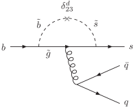
Figure 1: Gluino-squark loop penguin diagram.

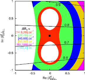
(a) Allowed region for $(\delta_{LL}^{d})_{23}$

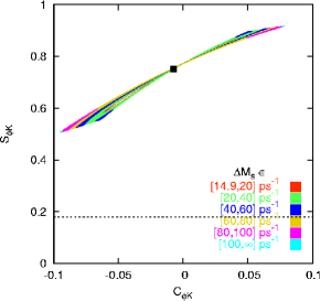
(b) $S_{\phi K}$ vs. $C_{\phi K}$

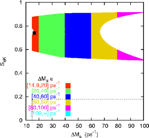
(c) $S_{\phi K}$ vs. $\Delta M_{s}$

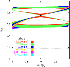
(d) $S_{\phi K}$ vs. $\sin 2\beta_{s}$

Figure 2: (a) Allowed region on the complex plane of $(\delta_{LL}^{d})_{23}$, and (b–d) correlations among observables for the $LL$ insertion case. Different shades are used for different values of $\Delta M_{s}$. The black square corresponds to the SM case. The dotted line represents the upper bound on $S_{\phi K}$ at 1-$\sigma$ level. Lines in Fig. (a) are contours of $S_{\phi K}$.

Here we adopt the mass insertion (MI) approximation which is one of the most convenient ways to analyzing this type of contribution. We consider four MI’s relevant to $b\rightarrow s$ transitions, i.e., $(\delta_{LL}^{d})_{23}$, $(\delta_{RR}^{d})_{23}$, $(\delta_{LR}^{d})_{23}$, and $(\delta_{RL}^{d})_{23}$, one at a time. In addition to these four cases, we include another one called $RL$ dominance scenario Everett:2001yy . In this case, $C_{7\gamma}$ and $C_{8g}$ are assumed to vanish at the $m_{b}$ scale, so the observed decay of $B\rightarrow X_{s}\gamma$ must come from $\widetilde{C}_{7\gamma}$, the chirality-flipped version of $C_{7\gamma}$. This unconventional scenario and the usual case can be distinguished by measuring the photon polarization. Therefore $(\delta_{RL}^{d})_{23}$ is forced to be a finite size to account for the data unlike the other four cases, and this corresponds to an extreme case with maximized SUSY effect in some sense. In the following, we turn on one of the four MI parameters at a time, and scan over it imposing constraints from $B\rightarrow X_{s}\gamma$ and $B_{s}$–$\overline{B_{s}}$ mixing as follows:

$$2.0\times 10^{-4}<B(B\rightarrow X_{s}\gamma)< 4.5\times 10^{-4},$$

$$\Delta M_{s}>14.9\ \text{ps}^{-1} \mbox{\cite[cite]{\@@bibref{Authors Phrase1YearPhrase2}{Stocchi:2000ps}{\@@citephrase{(}}{\@@citephrase{)}}}}.$$

We impose a rather generous bound on $B(B\rightarrow X_{s}\gamma)$ to take into account theoretical uncertainties. The common squark mass $\tilde{m}$ and the gluino mass $m_{\tilde{g}}$ are chosen to be $m_{\tilde{g}}=\tilde{m}=400$ GeV. We use QCD factorization Beneke:1999br in evaluating hadronic matrix elements for $B\to\phi K_{S}$. We do not assume any new physics in the $B^{0}$–$\overline{B}^{0}$ mixing because $\sin 2\beta$ measurement from the $B\rightarrow J/\psi K_{S}$ mode is well consistent with the SM fit.

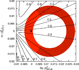
(a) Allowed region for $(\delta_{LR}^{d})_{23}$

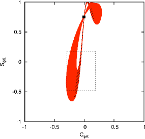
(b) $S_{\phi K}$ vs. $C_{\phi K}$

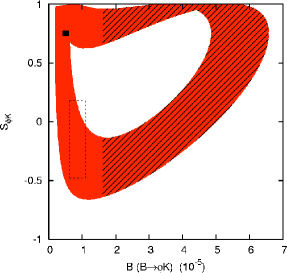
(c) $S_{\phi K}$ vs. $B(B\to\phi K_{S})$

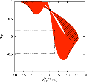
(d) $S_{\phi K}$ vs. $A_{\rm CP}^{b\to s\gamma}$

Figure 3: (a) Allowed region on the complex plane of $(\delta_{LR}^{d})_{23}$, and (b–d) correlations among observables for the $LR$ insertion case. The black square corresponds to the SM case. The dotted boxes represent current measurements at 1-$\sigma$ level. Lines in Fig. (a) are contours of $S_{\phi K}$.

First, let us consider the $LL$ insertion case. Fig. 2 (a) is the region of $(\delta_{LL}^{d})_{23}$ consistent with $B(B\rightarrow X_{s}\gamma)$ and $\Delta M_{s}$ constraints. The solid lines are contours of $S_{\phi K}$. The small square at the origin corresponds to the SM case, because there is no SUSY contribution there. The white space on the left is excluded by too small value of $B(B\rightarrow X_{s}\gamma)$. The two holes around the $\mathrm{Re}(\delta_{LL}^{d})_{23}=0$ line are excluded by too small $\Delta M_{s}$. In Fig. 2 (b), we plot predictions of $S_{\phi K}$ and $C_{\phi K}$ from the allowed values of $(\delta_{LL}^{d})_{23}$. The dotted horizontal line is the current 1-$\sigma$ upper limit on $S_{\phi K}$. This figure shows that the minimal value of $S_{\phi K}$ in this case is about +0.5, and the change of $S_{\phi K}$ from the SM prediction is not significant. Although $S_{\phi K}$ is not very much affected, large effect in $B_{s}$–$\overline{B_{s}}$ can be expected. For example, we show the prediction of $\Delta M_{s}$ in Fig. 2 (c). The SM value of $\Delta M_{s}$ is about 16 $\mathrm{ps}^{-1}$, marked by the black square. We can read huge enhancement of $\Delta M_{s}\sim 50\ \mathrm{ps}^{-1}$ is possible. Also, we show $\sin 2\beta_{s}$ in Fig. 2 (d), where $2\beta_{s}$ is the phase of $\langle B_{s}|H_{\mathrm{eff}}^{\Delta B=2}|\overline{B_{s}}\rangle$. The SM prediction of it is almost zero, but it can have any value between $-1$ and 1 here, which means that $CP$ violation in $B_{s}$–$\overline{B_{s}}$ mixing can drastically change.

The $RR$ insertion case is almost identical to the $LL$ insertion case. The only difference is the way $B(B\rightarrow X_{s}\gamma)$ constrains $(\delta_{RR}^{d})_{23}$. The $LL\ (RR)$ insertion mainly contributes to $C_{7\gamma}\ (\widetilde{C}_{7\gamma})$, and the dependence is such that

$$B(B\rightarrow X_{s}\gamma) \propto|C_{7\gamma}^{\mathrm{SM}}+C_{7\gamma}^{\mathrm{SUSY}}|^{2},\quad\text{for\ }LL,$$

$$B(B\rightarrow X_{s}\gamma) \propto|C_{7\gamma}^{\text{SM}}|^{2}+|\widetilde{C}_{7\gamma}^{\text{SUSY}}|^{2},\quad\text{for\ }RR.$$

Because of this difference, $(\delta_{RR}^{d})_{23}$ plane does not show a region excluded by $B(B\rightarrow X_{s}\gamma)$ that is present in Fig. 2 (a). However, this additional parameter space does not help shifting down $S_{\phi K}$ very much. Plots for this case are available in Ref. Kane:2002sp .

It is well known that the chirality-flipping $LR$ and $RL$ insertions receive enhancement by the factor of $m_{\tilde{g}}/m_{b}$, when they contribute to a (chromo) magnetic dipole operator. This is why they are strongly constrained by $B\rightarrow X_{s}\gamma$. For the same reason, they are more effective in modifying $S_{\phi K}$ and/or $C_{\phi K}$ than $LL$ or $RR$ insertion given the same magnitude of the MI parameter. We show the region of $(\delta_{LR}^{d})_{23}$ consistent with $B(B\rightarrow X_{s}\gamma)$ and $\Delta M_{s}$ in Fig. 3 (a). As in the previous case, the solid lines are contours of $S_{\phi K}$, and the small square at the origin corresponds to the SM case. The annulus with radius $\sim 10^{-2}$ comes from the $B(B\rightarrow X_{s}\gamma)$. Here the $B(B\rightarrow X_{s}\gamma)$ constraint is so strong that $\Delta M_{s}$ does not change very much from the SM value and play no role in constraining $(\delta_{LR}^{d})_{23}$. We show $S_{\phi K}$ and $C_{\phi K}$ from these values of $(\delta_{LR}^{d})_{23}$ in Fig. 3 (b). The dotted box is 1-$\sigma$ intervals of these observables, and we find some region where both $S_{\phi K}$ and $C_{\phi K}$ are within the box. This plot also shows a definite correlation between them. For $S_{\phi K}$ less (bigger) than the SM value, $C_{\phi K}<(>)\ 0$. Fig. 3 (c) is the plot of $B(B\to\phi K_{S})$, with hatches on the region where $B(B\to\phi K_{S})>1.6\times 10^{-5}$. This region, excluded by $B(B\to\phi K_{S})$ constraint, corresponds to the hatched region in Fig. 3 (a). Here we learn that significant portion of the $(\delta_{LR}^{d})_{23}$ parameter space that is consistent with $B(B\rightarrow X_{s}\gamma)$, is excluded by $B(B\to\phi K_{S})$. In Fig. 3 (d) is displayed the correlation between $S_{\phi K}$ and direct $CP$ asymmetry in $B\rightarrow X_{s}\gamma$. For $S_{\phi K}$ less (bigger) than the SM value, $A_{\rm CP}^{b\to s\gamma}>(<)\ 0$. It appears that $A_{\rm CP}^{b\to s\gamma}$ is outside the dotted box, but the experimental uncertainty is still large, so we cannot definitely conclude that this scenario is disfavored currently.

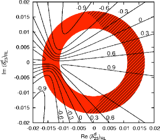
(a) Allowed region for $(\delta_{RL}^{d})_{23}$

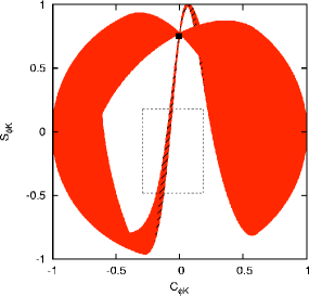
(b) $S_{\phi K}$ vs. $C_{\phi K}$

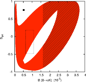
(c) $S_{\phi K}$ vs. $B(B\to\phi K_{S})$

Figure 4: (a) Allowed region on the complex plane of $(\delta_{RL}^{d})_{23}$, and (b–c) correlations among observables for the $RL$ dominance case. The black square corresponds to the SM case. The dotted boxes represent current measurements at 1-$\sigma$ level. Lines in Fig. (a) are contours of $S_{\phi K}$.

We turn to the $RL$ dominance scenario. Fig. 4 (a) is the region of $(\delta_{RL}^{d})_{23}$ constrained by $B(B\rightarrow X_{s}\gamma)$ and $\Delta M_{s}$. Again, the solid lines are contours of $S_{\phi K}$. In this case, we are assuming that SM contributions to $C_{7\gamma}$ and $C_{8g}$ are somehow canceled by SUSY contributions. Because we are always involving SUSY contributions in $C_{7\gamma}$ and $C_{8g}$, there cannot be any point on the $(\delta_{RL}^{d})_{23}$ plane that reduces to the SM case. The allowed annulus, centered at the origin, has radius $\sim 10^{-2}$, which is fixed by $B(B\rightarrow X_{s}\gamma)$. As in the previous case, the region consistent with $B(B\rightarrow X_{s}\gamma)$ is always consistent with $\Delta M_{s}$ as well. Predictions of $S_{\phi K}$ and $C_{\phi K}$ from the allowed region are shown in Fig. 4 (b). We can fit $S_{\phi K}$ to any value between $-1$ and 1. Moreover, big change in $C_{\phi K}$ from the SM value of zero, is expected in general, resulting in any value between $-1$ and 1. However, some region around the center is not covered. In Fig. 4 (c), we plot $B(B\to\phi K_{S})$, with hatches on the region with excessive $B(B\to\phi K_{S})$. Since there is only one weak phase in the $b\rightarrow s\gamma$ amplitude, we have $A_{\rm CP}^{b\to s\gamma}=0$ in this case. If we turned on another weak phase such as coming from $(\delta_{RR}^{d})_{23}$, we could have non-vanishing $A_{\rm CP}^{b\to s\gamma}$, but we do not pursue more detailed analysis here.

We also analyzed the usual $RL$ insertion case, keeping SM contributions to $C_{7\gamma}$ and $C_{8g}$. Because the SM prediction of $B(B\rightarrow X_{s}\gamma)$ is already consistent with the data, there is less room for new physics in this case than in the $RL$ dominance scenario. Nevertheless, we can get sizable change in $S_{\phi K}$, satisfying $B(B\rightarrow X_{s}\gamma)$. Plots for this case can be found in Ref. Kane:2002sp .

These results of analysis depend on the sparticle mass scale. For a fixed value of MI parameter, SUSY effects get enhanced as the sparticle masses decrease. In Figs. 5, we show possible values of $S_{\phi K}$ as functions of the gluino mass, $m_{\tilde{g}}$.

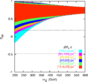
(a) $LL$ insertion case

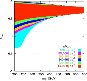
(b) $RR$ insertion case

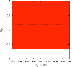
(c) $LR$ insertion case

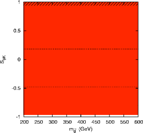
(d) $RL$ dominance case

Figure 5: Possible range of $S_{\phi K}$ as a function of the gluino mass. Different shades are used for different values of $\Delta M_{s}$. The dotted lines represent the current bounds on $S_{\phi K}$ at 1-$\sigma$ level.

In these plots, we fix the ratio $x\equiv m_{\tilde{g}}^{2}/\tilde{m}^{2}$ to be 1, and scan over one of the four MI parameters imposing constraints from $B(B\rightarrow X_{s}\gamma)$ and $\Delta M_{s}$. Figs. 5 (a) and (b) are for the chirality-preserving insertions, $LL$ and $RR$, respectively. Here we see a clear tendency of SUSY effects decoupling as the gluino mass increases. Note that our analysis shown in Figs. 2–4 is for $m_{\tilde{g}}=400$ GeV. The way to getting $S_{\phi K}$ consistent with the data is to imagine the gluino mass $\sim 250$ GeV, which is close to the current experimental lower bound. On the other hand, a chirality-flipping insertion, $LR$ or $RL$, shown in Figs. 5 (c) and (d), results in a range of $S_{\phi K}$ that is independent of $m_{\tilde{g}}$. This is explained in the following way in the $LR$ insertion case for example. The dependence of $B\rightarrow X_{s}\gamma$ on the SUSY parameters is only through the ratio of $(\delta_{LR}^{d})_{23}/m_{\tilde{g}}$, which precisely is the parameter that $S_{\phi K}$ also depends on. The set of $(\delta_{LR}^{d})_{23}/m_{\tilde{g}}$ allowed by $B(B\rightarrow X_{s}\gamma)$ is independent of $m_{\tilde{g}}$, and so is $S_{\phi K}$. The $RL$ and $RL$ dominance cases are explained likewise. In fact, this type of constant dependence would be true for $LL$ or $RR$ insertion case as well, if we allowed arbitrarily large size of $(\delta_{LL}^{d})_{23}$ or $(\delta_{RR}^{d})_{23}$ and if we discarded $\Delta M_{s}$ constraint.

In the QCD factorization, divergences coming from endpoint of integral $\int dx/x$ are regulated in the form of $X_{A(H)}=(1+\varrho_{A(H)}e^{i\varphi_{A(H)}})\ln(m_{B}/\Lambda_{h})$, where $\Lambda_{h}\sim 0.5$ GeV is the scale in hard-scattering. Discussion so far has been carried out without considering any uncertainties coming from this regularization, but we have to scan over the parameters $\varrho_{A,H}$ and $\varphi_{A,H}$ properly to take care of these theoretical uncertainties. In Fig. 6 (a), we show a curve of $S_{\phi K}$ as a function of the gluino mass. In this plot, we fix $x=1$, and turn on only the $RR$ insertion with the value $(\delta^{d}_{23})_{RR}=0.534-0.856i$, which minimizes $S_{\phi K}$ at $m_{\tilde{g}}=200$ GeV. This curve is broadened into bands shown in Fig. 6 (b), if we begin to scan over the aforementioned parameters. In general, the uncertainty in the annihilation from $\varrho_{A}$ dominates over that in hard spectator scattering from $\varrho_{H}$. The black band is for the range $0\leq\varrho_{A},\varrho_{H}\leq 1$, and this is what the authors of Ref. Beneke:1999br recommend to use. On this band, the tendency of decoupling SUSY effects with increasing $m_{\tilde{g}}$ is still maintained. However, for the case of $0\leq\varrho_{A},\varrho_{H}\leq 5$, which is displayed in light gray, estimated theoretical uncertainties are so large that almost every value of $S_{\phi K}$ between $-1$ and 1 is predicted, for any gluino mass between 200 GeV and 600 GeV. Ref. Ciuchini:2002uv claims that they get $S_{\phi K}<0$ from $LL$ or $RR$ insertion with $m_{\tilde{g}}=350$ GeV, disagreeing with us. We suspect this is due to the difference in choosing intervals for $\varrho_{A}$ and $\varrho_{H}$. They use $0\leq\varrho_{A}\leq 8$, and from Fig. 6 (b), it is obvious that $S_{\phi K}$ will have every value between $-1$ and 1 for this interval.

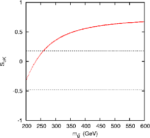
(a) $S_{\phi K}$ without hadronic uncertainties

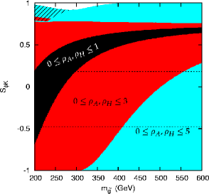
(b) $S_{\phi K}$ with hadronic uncertainties

Figure 6: Predictions of $S_{\phi K}$ from $(\delta^{d}_{23})_{RR}=0.534-0.856i$ as functions of the gluino mass, (a) with $X_{A}=X_{H}=0$, and (b) with varying $\varrho_{A},\varrho_{H}$. The dotted lines represent the current bounds on $S_{\phi K}$ at 1-$\sigma$ level. In Fig. (b), different shades are used for different ranges of $\varrho_{A}$ and $\varrho_{H}$.

Let us think of theoretical motivations for $(\delta_{LR}^{d})_{23}$ or $(\delta_{LR}^{d})_{23}\sim 10^{-2}$. In many alignment models using flavor symmetry, there remain small off-diagonal elements in the squark mass matrix in the super CKM basis. They can cause $(\delta^{d}_{23})_{LL}$ or $(\delta^{d}_{23})_{RR}$ $\sim 10^{-2}$ with arbitrary complex phase. This chirality preserving insertion can lead to an induced $LR$ or $RL$ insertion,

$$(\delta_{LR}^{d})_{23}^{\rm ind}=(\delta_{LL}^{d})_{23}\times{m_{b}(A_{b}-\mu\tan\beta)\over\tilde{m}^{2}}\sim 10^{-2},$$

provided $\tan\beta$ is large enough so that $\mu\tan\beta\sim 30$ TeV. This kind of double insertion mechanism has been used in explaining both $\epsilon_{K}$ and $\epsilon^{\prime}/\epsilon_{K}$ from a single $CP$ violation source of $(\delta_{LL}^{d})_{12}$ Baek:1999jq . We also constructed a model that naturally gives the desired amount of $LR$ or $RL$ insertion using intersecting D5 branes Kane:2002sp .

Since QCD penguin contributes to $b\rightarrow s\bar{q}q$ for $q=u,d,s,c,b$ at equal strength, one may worry about what happens to other decays such as $B\rightarrow\eta^{\prime}K_{S},\ \pi K,\ K^{+}K^{-}K_{S}$. There are other 4-quark operators which contribute only to these decays not affecting $B\to\phi K_{S}$, and changes in these decay modes are not definitely predictable in the present study. On the other hand, there is a nice mechanism which enables us to control $B\rightarrow VP$ and $B\rightarrow PP$ modes independently. Parity invariance tells us that the transition amplitudes of these modes depend on the new physics contribution in such a way that $B\rightarrow VP\ (PP)$ mode depends on $\sum_{i}[C^{\mathrm{NP}}_{i}+(-)\ \widetilde{C}^{\mathrm{NP}}_{i}]\,\#_{i}$, where $C^{\mathrm{NP}}_{i}$ and $\widetilde{C}^{\mathrm{NP}}_{i}$ are Wilson coefficients with opposite chiralities, coming from new physics. Hence we can control $B\rightarrow\eta^{\prime}K_{S}$ and $B\to\phi K_{S}$ separately, and only the latter will change if we imagine a situation where $(\delta_{LR}^{d})_{23}=(\delta_{RL}^{d})_{23}$, for instance. If this is the case, predictions of other observables such as $C_{\phi K}$ and $A_{\rm CP}^{b\to s\gamma}$ will be different than the four cases we considered here. After all, it requires further study to see changes in other decay modes in more general cases.

From now, we consider the neutral Higgs mediated contribution to $B\to\phi K_{S}$. A typical diagram is shown in Fig. 7.

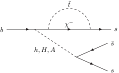
Figure 7: Higgs penguin diagram.

This diagram contributes to $B_{s}\rightarrow\mu^{+}\mu^{-}$ as well as to $B\to\phi K_{S}$ if we replace the $s\bar{s}$ pair with $\mu^{+}\mu^{-}$. Once we impose the upper bound from CDF Abe:1998ah , $B(B_{s}\rightarrow\mu^{+}\mu^{-})<2.6\times 10^{-6}$, we find that $S_{\phi K}>0.71$. This argument applies not only in minimal flavor violation scenario, but also in general MSSM Kane:2002sp . As a result, Higgs exchange does not cause substantial change in $S_{\phi K}$.

In conclusion, we analyzed SUSY contributions to time dependent $CP$ asymmetry in $B\to\phi K_{S}$. As to the gluino-squark loop, negative $S_{\phi K}$ is more likely to come from $LR$ or $RL$ insertion than from $LL$ or $RR$ insertion if the sparticle masses are not close to the current experimental lower bound. However, we may have chances to look for $LL$ or $RR$ insertion in $B_{s}$–$\overline{B_{s}}$ mixing. Correlations among $S_{\phi K}$, $C_{\phi K}$, $A_{\rm CP}^{b\to s\gamma}$, $\Delta M_{s}$, $\sin 2\beta_{s}$ may help us discriminate among different possibilities. Constraint from nonleptonic decays such as $B\to\phi K_{S}$ is becoming as severe as that from $B\rightarrow X_{s}\gamma$. Higgs mediated FCNC cannot explain $S_{\phi K}<0$. Finally, let us direct the reader to Ref. Kane:2002sp for more complete discussion including dilepton $CP$ asymmetry in $\Upsilon(4S)$ decay.

The author is grateful to G. L. Kane, P. Ko, C. Kolda, Haibin Wang, and Lian-Tao Wang, for enjoyable collaboration. This work was supported in part by KOSEF through CHEP at Kyungpook National University and by the BK21 program.

References

(1)
T. Browder, talk at Lepton Photon 2003, Fermilab, Aug. 11-16, 2003.
(2)
K. Abe et al. [Belle Collaboration],
hep-ex/0308035.
(3)
L. Everett, G. L. Kane, S. Rigolin, L. T. Wang and T. T. Wang,
JHEP 0201, 022 (2002).
(4)
A. Stocchi,
hep-ph/0010222.
(5)
M. Beneke, G. Buchalla, M. Neubert and C. T. Sachrajda,
Phys. Rev. Lett. 83, 1914 (1999);
Nucl. Phys. B 591, 313 (2000);
Nucl. Phys. B 606, 245 (2001).
(6)
G. L. Kane, P. Ko, H. b. Wang, C. Kolda, J.-h. Park and L. T. Wang,
hep-ph/0212092;
Phys. Rev. Lett. 90, 141803 (2003).
(7)
M. Ciuchini, E. Franco, A. Masiero and L. Silvestrini,
Phys. Rev. D 67, 075016 (2003)
[Erratum-ibid. D 68, 079901 (2003)].
(8)
S. Baek, J. H. Jang, P. Ko and J.-h. Park,
Phys. Rev. D 62, 117701 (2000);
Nucl. Phys. B 609, 442 (2001).
(9)
F. Abe et al. [CDF Collaboration],
Phys. Rev. D 57, 3811 (1998).