Toward understanding the lattice QCD results
from the strong coupling analysis

Abstract

This is a review of strong coupling approaches to grasp the nature of the phase transition in finite temperature and density QCD. We commence with classics of the center symmetry and the Polyakov loop in pure gauge theories. The effective action derived in the strong coupling limit gives qualitatively plausible behavior for the deconfinement transition at finite temperature. We can apply the strong coupling analysis to describe the chiral phase transition with the help of large dimensional expansion. In order to make this article as self-contained as possible, we elucidate the computational procedure and its physical meaning in detail. Also the relation between the Polyakov loop behavior and the chiral dynamics, the phase structure of two-color QCD, and future possibilities to be pursued in the strong coupling analysis are discussed.

1 Objectives

The aim we are trying to achieve here is to understand the phase structure of Quantum Chromodynamics (QCD) in a medium at finite temperature and baryon density. It is known that QCD would undergo phase transitions between different states of matter, namely, the hadronic phase, the quark-gluon plasma (color-deconfined or chiral symmetry restored phase) [1], the color-super conductivity or diquark super-fluidity [2], and some other exotic states like pion and kaon condensations, ferromagnetic spin alignment, etc.

The lattice QCD simulation is one of the most prosperous implements to draw the right answer among various possibilities [3]. The phase structure of QCD or QCD-like theories have been intensely investigated by the lattice simulation at finite temperature. In many cases the physical quantities of interest in the lattice calculation are the Polyakov loop and the chiral condensate. The Polyakov loop is supposed to be an order parameter characterizing the deconfinement transition [4, 5], as explained later. The chiral condensate is a familiar quantity serving as an order parameter for the chiral phase transition.

Even though we could extract the right answer from the lattice QCD results, we cannot reach a deep understanding of the QCD phase structure until we correctly comprehend, interpret and explain the numerical outputs. In a sense the lattice results may be regarded as experimental facts from which we should draw the physical meaning. For this purpose the effective model approach would be useful to abstract the essence. Also, on a technical level, model studies are indispensable particularly at finite baryon density because the lattice simulation cannot avoid suffering from the notorious negative sign problem of the Dirac determinant.

There are many successful effective models so far, such as the Nambu–Jona-Lasinio model [6], the linear sigma model [7], the chiral random matrix model [8], the instanton liquid model [9], the Polyakov loop model [10], and so on. In this review, we shall draw attention to another effective model description based on the strong coupling expansion. Even though the effective action given at strong coupling has no guarantee to lead to quantitative agreement with physical observables in the weak coupling regime, the strong coupling approach has advantages over other models as follows: 1) Because the effective model derived in the strong coupling expansion has an obvious connection to the fundamental theory, the result could be exact, in principle, in the limit of strong coupling. 2) The strong coupling expansion is the most natural approach on the lattice. Since it is formulated on the lattice, the correspondence to the lattice QCD simulation is transparent. 3) The strong coupling analysis is almost a unique method in which the chiral and the Polyakov loop dynamics are taken into account on equal footing. 4) The model parameters are few, namely, the lattice spacing $a$ and the current quark mass $m_{q}$. To our surprise, we can reach qualitative and even quantitative agreement with physical observables with these two parameters.

Figure 1: String tension in unit of the lattice spacing calculated up to twelfth order [11]. Two dashed curves represent the extreme cases of strong and weak coupling limits.

It should be noted here that we must be cautious about the continuity between the strong and weak coupling regions. If there is a phase transition at a certain value of the coupling constant, the strong coupling physics would not give any information on the weak coupling physics in reality. Although it is not resolved whether the strong coupling world is smoothly connected to the real world without any singularity, the string tension of the SU(2) gauge theory calculated up to twelfth order of the strong coupling expansion [11] suggests that physics continuously changes from the strong coupling limit toward the scaling limit in the perturbative regime (see Fig. 1).

2 Deconfinement and Chiral Restoration

The deconfinement phase transition is well-defined only in the pure gauge theory (gauge theory without quarks in the fundamental representation in color space). In this case we can determine whether the vacuum is a confined one or not by putting a test static color-charge. If the free energy gain $F_{\text{q}}$ diverges, any color-charge isolation is not allowed in this system so that confinement is realized. [If a theory contains dynamical quarks, $F_{\text{q}}$ is always finite due to string breaking effects. It is difficult then to characterize confinement by thermodynamic properties [12].]

$F_{\text{q}}$ can be calculated from the partition function with a test charge carried by a static quark $q^{\alpha}(\vec{r})$, which can be explicitly written down as [13, 5]

$$F_{\text{q}}(\vec{r})=-T\ln\int\mathcal{D}A_{i}\sum_{\alpha=1}^{N_{\text{c}}}\langle A_{i};q^{\alpha}(\vec{r})|\,\mathrm{e}^{-\beta H}\mathcal{P}|A_{i};q^{\alpha}(\vec{r})\rangle$$ (1)

in the Weyl gauge ($A_{0}=0$). $\mathcal{P}$ is the projection operator onto the physical state which should satisfy the Gauss law, that is;

$$\biggl{(}D_{i}\Pi_{A}^{i\alpha}-\mathrm{i}g\Pi_{q}\frac{\lambda^{\alpha}}{2}q\biggr{)}|A_{i};q^{\beta}(\vec{r})\rangle=\biggl{\{}D_{i}\Pi_{A}^{i\alpha}+g\frac{\lambda^{\alpha}}{2}\delta^{\alpha\beta}\delta(\vec{x}-\vec{r})\biggr{\}}|A_{i}\rangle=0$$ (2)

with the canonical momenta $\Pi_{A}^{i\alpha}$ and $\Pi_{q}$ for the gauge and quark fields respectively. $D_{i}$ stands for the covariant derivative. The Gauss law constraint needs a Lagrange multiplier which can be eventually regarded as $A_{4}$ (temporal component of the gauge field in Euclidean space-time) [14]. Then in the imaginary-time (Matsubara) formalism the free energy can be expressed as

$$F_{\text{q}}(\vec{r})\!=\!-T\ln\!\int\!\mathcal{D}A_{\mu}\,\mathrm{e}^{-S[A]}\,\mathrm{Tr_{c}}\mathcal{T}\exp\biggl{[}\mathrm{i}g\int_{0}^{\beta}\mathrm{d}x_{4}\,A_{4}(\vec{r},x_{4})\biggr{]}\!\equiv\!-T\ln\langle\mathrm{Tr_{c}}L(\vec{r})\rangle,$$ (3)

where $\mathcal{T}$ is time ordering and $\mathrm{Tr_{c}}$ is the trace in color space. The Polyakov loop is denoted by $L$. If we introduce a pair of test charge and anti-charge in the same way, we can attain the inter-quark potential, $F_{\mathrm{q\bar{q}}}$, expressed by the Polyakov loop correlation function. In Table 1 the basics on the Polyakov loop behavior are summarized.

	confined (disordered) phase	deconfined (ordered) phase
free energy	$F_{\text{q}}=\infty$	$F_{\text{q}}<\infty$
	$F_{\mathrm{q\bar{q}}}(\vec{r})\sim\sigma|\vec{r}|$	$F_{\mathrm{q\bar{q}}}(\vec{r})\sim-\mathrm{e}^{-m|\vec{r}|}/|\vec{r}|$
Polyakov loop	$\langle\mathrm{Tr_{c}}L\rangle=0$	$\langle\mathrm{Tr_{c}}L\rangle\neq 0$
	$\langle\mathrm{Tr_{c}}L^{\dagger}(0)\mathrm{Tr_{c}}L(\vec{r})\rangle\rightarrow 0$	$\langle\mathrm{Tr_{c}}L^{\dagger}(0)\mathrm{Tr_{c}}L(\vec{r})\rangle\nrightarrow 0\quad(|\vec{r}|\rightarrow\infty)$

Table 1: Confined and deconfined phases in the pure gauge theory.

As is clear in Table 1, the expectation value of the Polyakov loop serves as an order parameter to identify the deconfinement transition. In many cases a phase transition is linked with the spontaneous symmetry breaking. As a matter of fact, the Polyakov loop behavior is prescribed by the center symmetry [13, 5, 14]. The center symmetry in the SU($N_{\text{c}}$) gauge theory is defined by the gauge transformation satisfying a boundary condition twisted by an element, $z$, of the center Z($N_{\text{c}}$) [15]. The point is that such a gauge transformation does not affect the periodic boundary condition for the gauge field, while the Polyakov loop picks up the element $z$. As a result the expectation value of the Polyakov loop vanishes if the vacuum preserves the center symmetry. Hence, concerning the deconfinement transition, the SU($N_{\text{c}}$) gauge theory can be regarded as a spin system with the global Z($N_{\text{c}}$) symmetry described in terms of the Polyakov loop “spin” variables. The universality argument tells us the critical properties of the deconfinement transition which have been confirmed in the lattice simulations [3, 13, 16, 17].

One might have thought that it should be curious that the disordered (ordered) phase lies in the lower (higher) temperature side [18]. This seeming contradiction comes from the duality transformation connecting the gauge theory to a spin system. Going back to the original paper written by Polyakov [4], we can find the explicit transformation for the partition function (notation is slightly changed);

$$\int\mathcal{D}\phi\sum_{n}\exp\biggl{[}-\frac{g^{2}}{2T}\sum n_{x\mu}^{2}+\sum\mathrm{i}(\nabla n)\phi\biggr{]}\sim\int\mathcal{D}\phi\sum_{m}\exp\biggl{[}-\frac{T}{2g^{2}}\sum(\mathrm{i}\nabla\phi-2\pi m)^{2}\biggr{]}.$$ (4)

The left-hand-side is the partition function given by Hamiltonian in the strong coupling limit on the lattice. The electric flux string, $n_{x\mu}$, dominates over the magnetic fluctuation at strong coupling. The Gauss law is implemented by the Lagrange multiplier $\phi$ (that is $A_{4}$ in Eq. (3)). The right-hand-side is derived by Poisson’s resummation formula (duality transformation) up to an overall factor and is nothing but an approximated form of the XY spin model. From the above expression it can be clearly understood why the effective “spin” theory of the Polyakov loop has the inverse temperature.

In the rest of this section we shall briefly summarize the definitions inherent in the lattice description. The Wilson action of the gauge field is given by [19]

$$S_{\text{G}}[U]=\frac{2N_{\text{c}}}{g^{2}}\sum_{x,(\mu,\nu)}\biggl{\{}1-\frac{1}{N_{\text{c}}}\text{Re}\,\mathrm{Tr_{c}}\,U_{\mu\nu}(x)\biggr{\}}$$ (5)

with the plaquettes; $U_{\mu\nu}(x)=U_{\nu}^{\dagger}(x)U_{\mu}^{\dagger}(x+\hat{\nu})U_{\nu}(x+\hat{\mu})U_{\mu}(x)$. The coupling constant, $g^{2}$, only appears as an overall coefficient, from which the strong coupling expansion is derived. The Polyakov loop can be equivalently written on the lattice as

$$L(\vec{x})=\prod_{x_{d}=a}^{N_{\tau}a}U_{d}(\vec{x},x_{d})$$ (6)

in $d-$dimensional space-time. $N_{\tau}$ is the temporal extent and related to the temperature by $T=1/N_{\tau}a$ with the lattice spacing $a$.

As for the chiral symmetry, the lattice fermion suffers from the notorious species doubling problem. Among ideas to avoid having $2^{d}$-fold doublers, we shall limit our discussion in this review to the staggered formalism (Kogut-Susskind fermion [20]) that has advantage in providing a simple description of chiral symmetry. The staggered fermion $\chi(x)$ is derived from the Dirac fermion $\psi(x)$ by the following transformation;

$$\psi(x)=\Gamma(x)\chi(x),\quad\bar{\psi}(x)=\bar{\chi}(x)\Gamma^{\dagger}(x),\quad\Gamma(x)=\gamma_{1}^{x_{1}}\gamma_{2}^{x_{2}}\cdots\gamma_{d}^{x_{d}}.$$ (7)

Then Dirac’s gamma matrices are reduced to be unity and we can forget about the Dirac indices. As a result $2^{d}$-fold doublers are diminished by $2^{[d/2]}$. The remains are usually interpreted as flavor degrees of freedom. Since the flavor number might be sometimes confusing as it is, we will write $n_{\text{f}}$ to mean the original flavor number associated with staggered fermions and $N_{\text{f}}$ to mean the flavor number in the continuum limit (i.e., $N_{\text{f}}=4n_{\text{f}}$ for $d=4$).

It should be noted that the chiral symmetry is given by a U($n_{\text{f}}$)$\times$U($n_{\text{f}}$) rotation on alternate lattice sites. Although the symmetry pattern looks different, the chiral condensate, $\langle\bar{\chi}\chi\rangle$, serves as an order parameter for the chiral symmetry breaking; $\mathrm{U}(n_{\text{f}})\times\mathrm{U}(n_{\text{f}})\to\mathrm{U}_{\text{V}}(n_{\text{f}})$. The action for the staggered fermion is given by

$$S_{\text{F}}[U,\bar{\chi},\chi]=m_{q}\sum_{x}\bar{\chi}(x)\chi(x)+\frac{1}{2}\!\sum_{x,\mu>0}\eta_{\mu}(x)\bar{\chi}(x)\bigl{\{}U_{\mu}(x)\chi(x+\hat{\mu})-U_{\mu}^{\dagger}(x-\hat{\mu})\chi(x-\hat{\mu})\bigl{\}}$$ (8)

with $\eta_{\mu}(x)=(-1)^{x_{1}+x_{2}+\cdots x_{\mu-1}}$. The price for reducing spin indices is that the flavor contents are scattered and mixed on the adjacent lattice sites.

3 Deconfinement Transition

The lattice gauge theory was originally formulated by Wilson [19] with the aim of giving a plain explanation of color-confinement in the strong coupling limit. The strong coupling expansion on the lattice is achieved by statistical analog at high temperature. The formulation has been developed systematically. In this article we will not go into mathematical and technical details in general. If necessary, one can consult an exhaustive review written by Drouffe and Zuber [21].

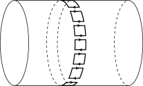
Figure 2: Leading-order contribution to the effective action with respect to the Polyakov loop. The cylinder represents temporal $S^{1}$ and spatial $R^{3}$ manifold.

In this section we shall focus on the strong coupling study on the deconfinement transition for which the order parameter is given by the Polyakov loop. We can attain the effective action in terms of the Polyakov loop by integrating over other degrees of freedom. As seen from (5), the large $g^{2}$ expansion is systematically available by the Taylor expansion of exponential of $S_{\text{G}}$. In the leading order of the strong coupling expansion the partition function with the Polyakov loop (or $U_{d}$) left unintegrated is calculated as (see Fig. 2)

$$Z_{\text{eff}}^{\text{(G)}}[U_{d}] =\int\mathcal{D}U_{i}\,\mathrm{e}^{-S_{\text{G}}[U_{i},U_{d}]}=\sum_{m=0}^{\infty}\frac{1}{m!}\int\mathcal{D}U_{i}\biggl{\{}\frac{1}{g^{2}}\sum_{x,(\mu,\nu)}\mathrm{Tr_{c}}\Bigl{(}U_{\mu\nu}(x)+U_{\mu\nu}^{\dagger}(x)\Bigr{)}\biggr{\}}^{m}$$

$$=1+\sum_{\vec{x},\hat{j}<d}\mathrm{Tr_{c}}\prod_{x_{d}=a}^{N_{\tau}a}U_{d}(\vec{x},x_{d})\,\mathrm{Tr_{c}}\prod_{x^{\prime}_{d}=a}^{N_{\tau}a}U_{d}^{\dagger}(\vec{x}+\hat{j}a,x_{d}^{\prime})\Bigl{(}\frac{1}{g^{2}N_{\text{c}}}\Bigr{)}^{N_{\tau}}+\text{(h.c.)}+\cdots.$$ (9)

Note that $1/N_{\text{c}}$ emerges as a result of the group integration. This expression immediately leads to the effective action as

$$S_{\text{eff}}^{\text{(G)}}[L]=-\ln Z_{\text{eff}}^{\text{(G)}}=-\mathrm{e}^{-\sigma a/T}\sum_{\text{n.n.}}\mathrm{Tr_{c}}L(\vec{x})\,\mathrm{Tr_{c}}L^{\dagger}(\vec{y}),$$ (10)

where n.n. is the abbreviation to mean the nearest-neighbor interaction. We have used $T=1/N_{\tau}a$ and the familiar expression of the string tension in the strong coupling limit; $\sigma a^{2}=\ln[g^{2}N_{\text{c}}]$.

The effective action (10) describes the $(d-1)$-dimensional classical spin system with the spin variable represented by $\mathrm{Tr_{c}}L$ and the exchange interaction by $\mathrm{e}^{-\sigma a/T}$ [22]. Although (10) looks quite simple, non-trivial complexity can originate from the matrix nature of the Polyakov loop. In the simplest mean-field analysis the matrix nature is taken into account by the Haar measure explicitly, that is the Jacobian associated with the variable transformation from $A_{4}$ to $L$ [23]. Then the effective potential can be approximated as

$$V_{\text{eff}}^{\text{(G)}}[L]/T=-2(d-1)\mathrm{e}^{-\sigma a/T}|\mathrm{Tr_{c}}L|^{2}-\ln\mathcal{M}_{\text{Haar}}[L],$$ (11)

where

$$\ln\mathcal{M}_{\text{Haar}}[L]=\begin{cases}\ln\bigl{[}1-|\mathrm{Tr_{c}}L/2|^{2}\bigr{]}&\text{for }N_{\text{c}}=2,\\ \ln\bigl{[}1\!-\!6|\mathrm{Tr_{c}}L/3|^{2}\!+\!8\text{Re}(\mathrm{Tr_{c}}L/3)^{3}\!-\!3|\mathrm{Tr_{c}}L/3|^{4}\bigr{]}&\text{for }N_{\text{c}}=3.\end{cases}$$ (12)

The effective potential for $N_{\text{c}}=2$ gives a second-order phase transition [24], while the Z(3) center symmetry allows a cubic term so that the phase transition is of first-order for $N_{\text{c}}=3$ [25]. Interestingly enough, it is obvious from (11) that confinement as well as the Z($N_{\text{c}}$) nature stem only from the Haar measure, as is consistent with the arguments that the Haar measure is essentially important for non-perturbative aspects of QCD [26].

Unfortunately straightforward generalization to $N_{\text{c}}>3$ cases is not available. Instead, as usually performed in the spin system, the Weiss approximation works well for arbitrary $N_{\text{c}}$. In this approximation, we take account of the fluctuation of the individual Polyakov loop surrounded by a constant mean field [21, 22, 27, 28, 29]. This results in a first-order phase transition for $N_{\text{c}}\geq 3$. In particular we can find the critical coupling $2(d-1)\mathrm{e}^{-\sigma a/T_{\text{d}}}=0.806$ for $N_{\text{c}}=3$. Once empirical values, the string tension $\sigma=(425\,\text{MeV})^{2}$ and the lattice spacing $a^{-1}=440\,\text{MeV}$ (see next section), are substituted, the deconfinement temperature is estimated as $T_{\text{d}}=204\,\text{MeV}$. One can, otherwise, fit the empirical value, $T_{\text{d}}=270\,\text{MeV}$, by choosing $a^{-1}=333\,\text{MeV}$ [29].

In short summary, the strong coupling expansion yields a simple form of the effective potential in terms of the Polyakov loop. It leads to even quantitatively acceptable results as well as qualitative agreement with gross features of the deconfinement transition. Since it is easy to handle, the effective potential (11) or more sophisticated one [28, 29] can also be a useful ingredient to build an effective model and probe underlying physics in model studies [30].

4 Chiral Phase Transition

4.1 Spontaneous chiral symmetry breaking at $T=\mu=0$

Now we shall deal with the system with dynamical quarks. The center symmetry is lost and the deconfinement transition is obscured then. Instead, the chiral symmetry plays an important role. In this subsection we will describe the spontaneous chiral symmetry breaking at $T=\mu=0$ mainly according to the formalism given by Kawamoto and Smit [31] and Kluberg-Stern, Morel and Petersson [32].

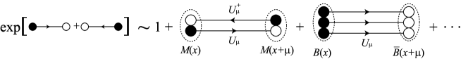
Figure 3: Intuitive graphical representation of the $U_{\mu}$ integration.

In the $g^{2}\to\infty$ limit the gauge action can be neglected. We can accomplish the integration with respect to $U_{\mu}$ on each lattice site by expanding the exponential of (8). Such series of the Taylor expansion corresponds to the large dimensional expansion, as explained below. For our present purpose to explain how it works, we only keep the leading order contributions. Then the $U_{\mu}$ integration picks up the mesonic and baryonic (color-singlet) composites as (see Fig. 3)

$$\int\mathrm{d}U_{\mu}(x)\;\exp\biggl{[}-\frac{1}{2}\eta_{\mu}(x)\bar{\chi}(x)U_{\mu}(x)\chi(x+\hat{\mu})+\frac{1}{2}\eta_{\mu}(x+\hat{\mu})\bar{\chi}(x+\hat{\mu})U_{\mu}^{\dagger}(x)\chi(x)\biggr{]}$$

$$=1+\frac{N_{\text{c}}}{2d}\mathrm{Tr_{f}}M(x)M(x+\hat{\mu})+\cdots$$

$$\>-\!(-1)^{N_{\text{c}}(N_{\text{c}}-1)/2}\biggl{\{}\frac{\eta(x)}{2\sqrt{d}}\biggr{\}}^{N_{\text{c}}}\!\!\mathrm{Tr_{f}}\bigl{\{}\bar{B}(x\!+\!\hat{\mu})B(x)\!+\!(-1)^{N_{\text{c}}}\bar{B}(x)B(x\!+\!\hat{\mu})\bigr{\}}+\cdots,$$ (13)

where the mesonic and baryonic composites with flavor indices are defined by

$$\begin{split}&M_{ij}(x)=\frac{1}{N_{\text{c}}}\sqrt{\frac{d}{2}}\sum_{\alpha=1}^{N_{\text{c}}}\chi_{i}^{\alpha}\bar{\chi}_{j}^{\alpha}(x),\\ &B_{i_{1}i_{2}\cdots i_{N_{\text{c}}}}(x)=\frac{d^{N_{\text{c}}/4}}{N_{\text{c}}!}\sum_{\alpha_{1},\dots,\alpha_{N_{\text{c}}}=1}^{N_{\text{c}}}\epsilon_{\alpha_{1}\alpha_{2}\cdots\alpha_{N_{\text{c}}}}\chi_{i_{1}}^{\alpha_{1}}\chi_{i_{2}}^{\alpha_{2}}\cdots\chi_{i_{N_{\text{c}}}}^{\alpha_{N_{\text{c}}}}(x).\end{split}$$ (14)

Here we can understand where the $1/d$ expansion emerges from. The large $d$ limit would make sense under the condition that the mesonic propagation has a finite amplitude. Since the index $\mu$ runs over $d$ directions, the hopping term $M(x)M(x+\hat{\mu})$ should be divided by $d$. In other words, the quark fields, $\chi$ and $\bar{\chi}$, should be normalized by $d^{1/4}$ like (14). Consequently, the Taylor expansion in terms of $\chi$ and $\bar{\chi}$ leads to the systematic $1/d$ expansion.

Although the baryonic term may be important when the system has a non-vanishing baryon chemical potential, we shall drop it from (13) and examine the spontaneous breaking of chiral symmetry. [Note that the baryonic term is of higher order in the $1/d$ expansion for $N_{\text{c}}\geq 3$.] In order to transform variables from the quark fields $\chi$ to the meson field $\lambda$, we linearize the four-fermionic interaction by inserting an auxiliary field in the following way;

$$\exp\biggl{[}N_{\text{c}}\sum_{x,y}\mathrm{Tr_{f}}\biggl{\{}\frac{1}{2}M(x)V_{M}(x,y)M(y)+2\bar{m}_{q}M(x)\delta_{xy}\biggr{\}}\biggr{]}$$

$$= \int\mathcal{D}\lambda\;\exp\biggl{[}-N_{\text{c}}\sum_{x,y}\mathrm{Tr_{f}}\biggl{\{}\frac{1}{2}\lambda(x)V_{M}(x,y)\lambda(y)-\bigl{(}\lambda(x)V_{M}(x,y)+2\bar{m}_{q}\delta_{x,y}\bigr{)}M(y)\biggr{\}}\biggr{]},$$ (15)

where $V_{M}(x,y)=(1/2d)\sum_{\mu}(\delta_{x,y+\hat{\mu}}+\delta_{x,y-\hat{\mu}})$ represents the mesonic hopping propagation between the nearest neighbor sites and $\bar{m}_{q}=m_{q}/\sqrt{2d}$.

Now that the effective action is linearized in regard to the composite field $M(x)$, the integration with respect to the quark fields, $\chi(x)$, is straightforward to be carried out resulting in the effective action in terms of $\lambda(x)$;

$$S_{\text{eff}}^{\text{(F)}}[\lambda]=\frac{N_{\text{c}}}{2}\sum_{x,y}\mathrm{Tr_{f}}\lambda(x)V_{M}(x,y)\lambda(y)-N_{\text{c}}\sum_{x}\mathrm{Tr_{f}}\ln\Bigl{[}\sum_{y}\lambda(y)V(y,x)+2\bar{m}_{q}\Bigr{]}.$$ (16)

Here $\lambda$ can be regarded as the meson field and its condensate, which is denoted by $\delta^{ij}\bar{\lambda}$, generates an additional contribution to the quark mass. The stationary value of $\bar{\lambda}$ is fixed by the extremal condition of the effective potential,

$$V_{\text{eff}}^{\text{(F)}}[\bar{\lambda}]=\frac{N_{\text{c}}n_{\text{f}}}{2}\bar{\lambda}^{2}-N_{\text{c}}n_{\text{f}}\ln\bigl{[}\bar{\lambda}+2\bar{m}_{q}\bigr{]},$$ (17)

to lead to a finite scalar condensate, $\bar{\lambda}=-\bar{m}_{q}+\sqrt{1+\bar{m}_{q}^{2}}$, which brings about the spontaneous breaking of chiral symmetry. Actually $\bar{\lambda}$ is directly related to the chiral condensate,

$$\Psi_{q}=\langle\bar{\chi}(x)\chi(x)\rangle=-\frac{1}{N^{d}N_{\text{c}}n_{\text{f}}}\cdot\frac{\mathrm{d}}{\mathrm{d}m_{q}}\ln\int\mathcal{D}\lambda\;\mathrm{e}^{-S_{\text{F}}[\lambda]},$$ (18)

by a simple proportionality relation; $\Psi_{q}=-\bar{\lambda}\sqrt{2/d}$ (see a reference [29] for details). We should remark that the logarithmic term in the effective potential (17) makes infinite barrier around the symmetric vacuum ($\bar{\lambda}=\bar{m}_{q}=0$) and this logarithmic singularity alone is responsible for the symmetry breaking in the present approach.

In the next place let us look into the meson spectrum acquired in this framework. The kinetic term of the meson fluctuation, $\delta\lambda(x)$, around the stationary condensate provides us with the propagator of meson excitations, whose poles correspond to the dispersion relations physical particles should satisfy. From the effective action (16) we have the kinetic term as

$$-\frac{N_{\text{c}}}{2}\sum_{x,y}\mathrm{Tr_{f}}\delta\lambda(x)\Bigl{\{}V_{M}(x,y)+\frac{1}{(\bar{\lambda}+2\bar{m}_{q})^{2}}V_{M}^{2}(x,y)\Bigr{\}}\delta\lambda(y).$$ (19)

To derive the information on the meson spectrum we transform the meson propagator into the representation in the momentum space. Then the inverse propagator is

$$\frac{N_{\text{c}}}{(\bar{\lambda}+2\bar{m}_{q})^{2}}\sum_{x,y}\mathrm{e}^{\mathrm{i}kx}V_{M}(x,y)\bigl{\{}(\bar{\lambda}+2\bar{m}_{q})^{2}\delta_{y0}+V_{M}(y,0)\bigr{\}}$$

$$\propto\;\; \tilde{V}_{M}(k)\bigl{\{}(\bar{\lambda}+2\bar{m}_{q})^{2}+\tilde{V}_{M}(k)\bigr{\}}\;\propto\;\frac{1}{d}\sum_{\mu}\cos k_{\mu}+(\bar{\lambda}+2\bar{m}_{q})^{2},$$ (20)

where we used the Fourier transformed hopping propagator in the momentum space, $\tilde{V}_{M}(k)$, which is obtained as

$$\tilde{V}_{M}(k)=\sum_{x}\mathrm{e}^{\mathrm{i}kx}V_{M}(x,0)=\frac{1}{d}\sum_{\mu}\cos k_{\mu}.$$ (21)

Now that the meson propagator in the momentum space is known, we can read the meson masses putting the momentum $k_{\mu}=(\vec{0},\mathrm{i}M)+\pi\delta_{\mu}$ into the propagator. The last term $\delta_{\mu}$ takes either $1$ or $0$ representing the fermion doublers which are absorbed into the flavor degrees of freedom. From the condition that the inverse of the meson propagator has zeros, we have the meson spectrum in the present approach as

$$\cosh M_{p}=d\{(\bar{\lambda}+2\bar{m}_{q})^{2}-1\}+2p+1.\qquad(p=0,1,\dots,d-1)$$ (22)

$M_{0}$ and $M_{1}$ are identified as the masses of the lightest state belonging to $0^{-}$ (pion) and mainly $1^{-}$ ($\rho$ meson), respectively. $M_{2}$ and $M_{3}$ are regarded as $1^{+}$ ($a_{1}$ meson) and $0^{+}$ ($a_{0}$ meson) with significant mixtures with $1^{-}$ and $0^{-}$ [33]. In order to reproduce the physical values, $m_{\pi}=140\;\text{MeV}$ and $m_{\rho}=780\;\text{MeV}$ , the model parameters are fixed as

$$m_{q}=8\;\text{MeV},\qquad a^{-1}=440\;\text{MeV},$$ (23)

which give other physical quantities as listed in Table 2. We would like to conclude this subsection with quoting from Kluberg-Stern et al. – “We believe that this is not a bad result owing to the crudeness of the model.”

	$g^{2}=0$	Physical values
$M_{2}$	$910\;\text{MeV}$	$m_{a_{1}}=1260\;\text{MeV}$
$M_{3}$	$1010\;\text{MeV}$	$m_{a_{0}}=980\;\text{MeV}$
$M_{\text{B}}$	$1380\;\text{MeV}$	$m_{N}=940\;\text{MeV}$
$\Psi_{q}$	$-(390\;\text{MeV})^{3}$	$-(240\;\text{MeV})^{3}$
$f_{\pi}$	$190\;\text{MeV}$	$93\;\text{MeV}$

Table 2: Hadron spectrum inferred from the strong coupling analysis. The baryon mass, $M_{\text{B}}$, can be obtained by inserting the baryonic auxiliary field to (13) and $f_{\pi}$ from the PCAC relation.

4.2 Chiral restoration at $T\neq 0$ and $\mu\neq 0$

Since the $1/d$ expansion works quite well to describe the spontaneous chiral symmetry breaking at zero temperature, it is interesting to see what kind of phase structure appears at finite temperature and baryon density. The extension to the evaluation in a hot and dense medium is straightforward as found in literatures [28, 29, 34]. The temperature dependence originates from the boundary condition in the temporal direction and the baryon chemical potential dependence is introduced by the replacement; $U_{d}\to\mathrm{e}^{\mu}U_{d}$ ($\mu$ being the quark chemical potential) [35]. These facts suggest that we should carefully treat the integration along the temporal direction apart form the others in the spatial $(d-1)$-dimensional coordinates. We have two strategies to embody it.

One is a physically preferable but technically difficult method. First, all $U_{\mu}$ (including $U_{d}$) are integrated by means of the $1/d$ expansion. The resultant action is (13) with the baryonic term in the temporal direction multiplied by $\mathrm{e}^{N_{\text{c}}\mu}$. Then, after inserting the mesonic and baryonic auxiliary fields ($\lambda$ and $b$), the integrations with respect to $\chi$ and $b$ are performed to obtain the effective potential in terms of $\lambda$. This computational procedure works well at $T=0$ and $\mu\neq 0$. The physical intuition that the $\mu$ dependence comes from the baryonic excitations would make sense. Unfortunately for the $T\neq 0$ system, however, we have to take account of not only the baryonic but also the mesonic loops explicitly and the calculation becomes too complicated.

The other is much simpler to handle. First, $U_{d}$ are left unintegrated and the $1/d$ expansion is applied only for the $U_{i}$ integration. Then, after inserting $\lambda$, the integration with respect to $\chi$ and $U_{d}$ are exactly carried out. It should be mentioned that in this method the baryonic term in (13) is not necessary to deal with the $\mu$ dependence. In principle, the $\chi$ integration with unintegrated $U_{d}$ contains in itself the thermal excitation of both mesonic and baryonic composite states. The problem is that the physical meaning is not transparent especially in the confined phase because the thermal excitation is given by quarks in this method.

Here we will explain the latter method in detail neglecting the baryonic hopping term. The integration over $U_{i}(x)$ is done by the same procedures as in the case at zero temperature. Then the partition function can be written as

$$\int\!\mathcal{D}U_{d}\mathcal{D}\chi\mathcal{D}\bar{\chi}\,\exp\biggl{[}-\frac{1}{2}\sum_{x}\eta_{d}(x)\bar{\chi}(x)\bigl{\{}\mathrm{e}^{\mu}U_{d}(x)\chi(x\!+\!\hat{d})-\mathrm{e}^{-\mu}U_{d}^{\dagger}(x\!-\!\hat{d})\chi(x\!-\!\hat{d})\bigr{\}}$$

$$\qquad-\frac{N_{\text{c}}}{2}\sum_{x,y}\lambda(x)V_{M}(x,y)\lambda(y)+N_{\text{c}}\sum_{x,y}\bigl{(}\lambda(x)V_{M}(x,y)+2\bar{m}_{q}\delta_{x,y}\bigr{)}M(y)\biggr{]},$$ (24)

where $V_{M}(x,y)$ represents the hopping propagator only in the spatial directions. In the mean-field approximation the meson field, $\lambda(x)$, is simply replaced by constant $\delta^{ij}\bar{\lambda}$. Then the functional integration with respect to the quark field, $\chi(x)$, is reduced into the one-dimensional problem and it can be easily manipulated. After the $\chi$ integration, the expression is simplified as

$$\int\mathcal{D}U_{d}\prod_{\alpha=1}^{N_{\text{c}}}\Bigl{[}2\cosh(N_{\tau}E)+2\cos(\theta_{\alpha}-\mathrm{i}\mu)\Bigr{]}^{n_{\text{f}}}$$ (25)

in the Polyakov loop gauge ($U_{d}=\text{diag}(\mathrm{e}^{\mathrm{i}\theta_{1}},\dots,\mathrm{e}^{\mathrm{i}\theta_{N_{\text{c}}}})$). For simplicity we will focus on the $n_{\text{f}}=1$ case ($N_{\text{f}}=4$) from now on. Then the integration with respect to $\chi$ results in the effective potential;

$$V_{\text{eff}}^{\text{(F)}}[\lambda]=\frac{N_{\text{c}}}{2}\bar{\lambda}^{2}-\frac{1}{N_{\tau}}\ln\Biggl{[}2\cosh(N_{\tau}N_{\text{c}}\mu)+\frac{\sinh[(N_{\text{c}}+1)N_{\tau}E]}{\sinh(N_{\tau}E)}\Biggr{]}$$ (26)

with the definition; $E=\sinh^{-1}(\bar{\lambda}\sqrt{(d-1)/2}+m_{q})$.

Now we can draw the phase diagram derived from (26) with $m_{q}=0$ (chiral limit) and $N_{\text{c}}=3$. As long as $\mu$ is not large, the chiral phase transition is of second-order. The phase boundary can be determined by the condition that the potential curvature around $\bar{\lambda}=0$ (denoted by $C_{0}$) passes across zero. When $\mu$ gets larger, the phase transition becomes of first-order. As a result we reach the phase structure depicted in Fig. 4. What seems interesting is that in some region of $\mu$ the chiral phase transition undergoes twice with increasing temperature unlike the results in other model studies.

Figure 4: Phase diagram derived from (26) with $m_{q}=0$ and $N_{\text{c}}=3$ in unit of the lattice spacing. $C_{0}$ is the potential curvature at $\bar{\lambda}=0$. Thick dashed and solid curves represent the second and first order boundaries respectively.

5 Relation between Two Phase Transitions

In the last section we have seen that the $U_{d}$ integration is dealt with separately. Since the Polyakov loop consists of $U_{d}$, it is easy to put the Polyakov loop into the formalism. Once we construct an effective model with the chiral order parameter and the Polyakov loop, we can investigate the relation between the deconfinement and chiral phase transitions. An interesting question is why these two transitions have been observed at the same temperature in the lattice QCD simulations [17, 36].

The effect of dynamical quarks on the deconfinement phase transition was first studied by Green and Karsch [37] with the hopping parameter (heavy quark) expansion. Chiral symmetry was seriously taken into account by Gocksch and Ogilvie [28], followed by the finite density extension by Ilgenfritz and Kripfganz [38]. The Gocksch-Ogilvie model is defined by the effective action; [29]

$$\begin{split}&S_{\text{eff}}[L,\lambda]=-\mathrm{e}^{-\sigma a/T}\sum_{\text{n.n.}}\mathrm{Tr_{c}}L(\vec{x})\mathrm{Tr_{c}}L^{\dagger}(\vec{y})\\ &\qquad+\frac{N_{\text{c}}}{2}\sum_{x,y}\lambda(x)V_{M}(x,y)\lambda(y)-\frac{N_{\text{f}}}{4}\sum_{\vec{x}}\mathrm{Tr_{c}}\ln\biggl{[}\cosh(N_{\tau}E)+\frac{1}{2}(L+L^{\dagger})\biggr{]}.\end{split}$$ (27)

This can be understood as a combination of (10) and (26). The effective potential $V_{\text{eff}}[l,\bar{\lambda}]$ ($l$ being the expectation value of the Polyakov loop) obtained from (27) in the mean-field approximation has an interesting property, that is, $V_{\text{eff}}[l=0,\bar{\lambda}]$ inevitably has instability at $\bar{\lambda}=0$ and thus it leads to a non-vanishing chiral condensate. Roughly speaking, the confined vacuum breaks chiral symmetry at any temperature. As emphasized in a chiral effective model study with the Polyakov loop [30], this property suggests $T_{\chi}\geq T_{d}$ (the chiral restoration temperature is higher than the deconfinement temperature). Remembering that $T_{d}\sim 270\;\text{MeV}$ without dynamical quarks is higher than $T_{\chi}\sim 150\;\text{MeV}$, we can expect to have $T_{d}=T_{\chi}$ in the presence of dynamical quarks. As a matter of fact, we can see that in the Gocksch-Ogilvie model the simultaneous crossovers are attributed to this mechanism, as shown in the left of Fig. 5.

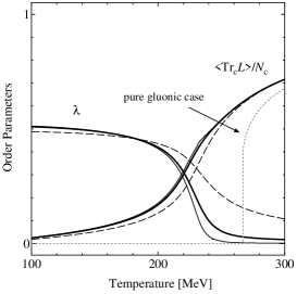
Figure 5: The Polyakov loop and the chiral order parameter as functions of the temperature calculated in the Gocksch-Ogilvie model [29]. The left figure is for the system with dynamical quarks in the fundamental representation in color space. The right figure is for the system with adjoint quarks. Thick curves are for the physical value of the quark mass and thin solid and dashed curves are for $m_{q}=1\;\text{MeV}$ and $m_{q}=50\;\text{MeV}$ respectively.

6 QCD-like Theories

6.1 QCD with Adjoint Quarks (aQCD)

Adjoint quarks have the same color structure as gluons and thus never break the center symmetry. In the lattice simulation of QCD with adjoint quarks (aQCD), as expected, the deconfinement transition is found to be of first-order [39]. The Gocksch-Ogilvie model has been generalized to include adjoint quarks and the model study gives a satisfactory explanation on all the qualitative features [29]. The right of Fig. 5 is the result in the Gocksch-Ogilvie model with adjoint quarks.

6.2 Two-Color QCD

Two-color QCD (QCD with $N_{\text{c}}=2$) has special properties. As explained before, the staggered fermion has the global $\mathrm{U}(n_{\text{f}})\times\mathrm{U}(n_{\text{f}})$ symmetry for $m_{q}=0$. For $N_{\mathrm{c}}=2$, the chiral symmetry is graded to U($2n_{\text{f}}$) [40, 32]. This is because the color SU(2) group is pseudo-real and the action possesses Pauli-Gürsey’s symmetry [41], which also makes possible the lattice simulation at finite density.

Introduction of a finite chemical potential $\mu$ or quark mass $m_{q}$ explicitly breaks the U(2$n_{\text{f}}$) symmetry. Listed in Table 3 are the symmetries realized in various circumstances and their breaking patterns for $n_{\text{f}}=1$.

	$m=0$	$m\neq 0$
$\mu=0$	U(2)	$\mathrm{U_{V}(1)}$
	broken to U(1) with 3 NG modes	not broken
$\mu\neq 0$	$\mathrm{U_{V}(1)\times U_{A}(1)}$	$\mathrm{U_{V}(1)}$
	totally broken with 2 NG modes	totally broken with 1 NG mode

Table 3: Symmetry realized in the single-component staggered-fermion action for $N_{\text{c}}=2$. Possible symmetry breaking patterns and the number of Nambu-Goldstone (NG) modes are also listed.

To our surprise, the chiral condensate, $\langle\bar{\chi}\chi\rangle$, of two-color QCD vanishes in the chiral limit ($m_{q}=0$). Instead, the diquark condensate, $\langle\chi\chi\rangle$, plays an important role. Note that $\chi\chi\equiv\epsilon_{\alpha\beta}\chi^{\alpha}\chi^{\beta}$ is a gauge invariant operator for $N_{\text{c}}=2$ and it corresponds to the baryonic contribution in (13). The phase structure was first investigated in the strong coupling approach by Dagotto, Karsch and Moreo [42]. The analytical and numerical studies have been inexhaustively explored within the framework of the strong coupling limit [43, 44]. The results are consistent with the lattice simulation [45]. The order parameters and the phase diagram are shown in Fig. 6.

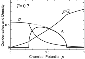
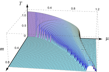
Figure 6: Left: Chiral and diquark condensates ($\sigma$ and $\Delta$ respectively) for $m_{q}=0.02$. Dotted curve represents the magnitude of condensation; $\sqrt{\sigma^{2}+\Delta^{2}}$. The mixing angle between $\sigma$ and $\Delta$ is controlled by $m_{q}$. If $m_{q}=0$ then $\sigma=0$ and the condensation is saturated by $\Delta$. Right: Phase boundaries in the 3-dimensional $(m_{q},T,\mu)$ space. Below the critical surface, $\Delta$ takes a non-vanishing value [44].

7 Beyond Understanding

We have looked over various aspects of the strong coupling approach to QCD. Since the celebrated paper by Wilson, there are quite a few contributions to clarify QCD physics in the strong coupling limit. Nevertheless, there still remain several interesting questions to be answered in the strong coupling analysis. We shall enumerate some possibilities here;

1) Glueballs at finite temperature – In the pure gauge theory, the Polyakov loop is an order parameter for the deconfinement transition. However, the physical interpretation and the dynamical description (real-time evolution) of the Polyakov loop are not clear in Minkowski space-time. In principle, we can define the deconfinement transition in terms of physical excitations, namely, glueballs [46]. At zero temperature, glueballs are well described in the strong coupling expansion [47]. A finite-temperature extension would give us concrete information on electric and magnetic glueballs near the deconfinement transition temperature [48].

2) Relation between the deconfinement and chiral phase transitions at finite density – Since the lattice QCD simulation has given no definite answer at finite density, the model study preceding future lattice simulations at finite density would be especially useful. Because, unlike the temperature, the baryon density effect explicitly breaks the center symmetry, it could be expected that the Polyakov loop behavior should be significantly affected at finite density.

3) Color-super conductivity on the lattice [50] – Although the lattice simulation is not applicable at finite density, we believe that the sign problem could be gotten over someday. Then an interesting and important problem would be how to see the color-super conductivity on the lattice. Because of Elitzur’s theorem [49], we have to make a gauge invariant order parameter or choose a certain gauge fixing condition.

4) Phase structure of the system at finite isospin density – It is interesting to apply the strong coupling approach to investigate the phase transition at finite isospin density [51], for there are numerical outputs from the lattice simulation [52]. In order to incorporate the flavor structure the Wilson fermion is more suitable then. The strong coupling analysis with Wilson fermions should be developed [53].

Beyond understanding the existing lattice data, we would like to emphasize that the strong coupling analysis could be a powerful tool to give some guideline or prediction to future progress in the lattice approaches. I hope that this contribution presented here will provide some clues to open the way for finite density QCD.

References

- [1] For a review on the quark-gluon plasma, see: D.H. Rischke, arXive: nucl-th/0305030.
- [2] For a review on the color-super conductivity, see: K. Rajagopal and F. Wilczek, in At the Frontier of Particle Physics: Handbook of QCD, ed. M. Shifman (World Scientific Singapore, 2001), arXive: hep-ph/0011333.
- [3] For reviews on the lattice simulation, see: E. Laermann and O. Philipsen, arXive: hep-ph/0303042. S. Muroya, A. Nakamura, C. Nonaka and T. Takaishi, \PTP110,2003,615.
- [4] A.M. Polyakov, \PLB72,1978,477. L. Susskind, \PRD20,1979,2610.
- [5] For reviews on the Polyakov loop and the center symmetry, see: B. Svetitsky, \PRP132,1986,1. R.D. Pisarski, arXive: hep-ph/0203271.
- [6] Y. Nambu and G. Jona-Lasinio, \JLPhys. Rev. ,122,1961,345; \andvol124,1961,246.
- [7] B.W. Lee, Chiral Dynamics (Gordon and Breach, New York, 1972).
- [8] E. Shuryak and J.J.M. Verbaarschot, \NPA560,1993,306.
- [9] T. Schäfer and E.V. Shuryak, \JLRev. Mod. Phys.,70,1998,323.
- [10] R.D. Pisarski, \PRD62,2000,111501.
- [11] G. Münster, \NPB180,1981,23.
- [12] K. Fukushima, \ANN304,2003,72.
- [13] B. Svetitsky and L.G. Yaffe, \NPB210,1982,423; \PRD26,1982,963. L.D. McLerran and B. Svetitsky, \PLB98,1981,195; \PRD24,1981,450. J. Kuti, J. Polonyi and K. Szlachanyi, \PLB98,1981,199.
- [14] D.J. Gross, R.D. Pisarski and L.G. Yaffe, \JLRev. Mod. Phys.,53,1981,43.
- [15] ’t Hooft, \NPB138,1978,1; \NPB153,1979,141.
- [16] J. Engels, F. Karsch, H. Satz and I. Montvay, \PLB101,1981,89. R.V. Gavai, \NPB215,1983,458. R.V. Gavai, F. Karsch and H. Satz, \NPB220,1983,223. J. Engels, J. Fingberg and M. Weber, \NPB332,1990,737. J. Engels, J. Fingberg and D.E. Miller \NPB392,1993,493.
- [17] J. Kogut, M. Stone, H.W. Wyld, W.R. Gibbs, J. Shigemitsu, S.H. Shenker and D.K. Sinclair, \PRL50,1983,393.
- [18] A.V. Smilga, \PRP291,1997,1.
- [19] K. Wilson, \PRD10,1974,2445.
- [20] J. Kogut and L. Susskind, \PRD11,1975,395.
- [21] J.M. Drouffe and J.B. Zuber, \PRP102,1983,1.
- [22] J. Kogut, M. Snow and M. Stone, \NPB200,1982,211.
- [23] H. Reinhardt, \JLMod. Phys. Lett. A,11,1996,2451.
- [24] J. Polónyi and K. Szlachányi, \PLB110,1982,395.
- [25] M. Gross, \PLB132,1983,125. M. Gross, J. Bartholomew, and D. Hochberg, “SU() Deconfinement Transition and the State Clock Model,” Report No. EFI-83-35-CHICAGO.
- [26] A. Gocksch and R.D. Pisarski, \NPB402,1993,657. F. Lentz and M. Thies, \ANN268,1998,308.
- [27] M. Creutz, Quarks, gluons and lattices, (Cambridge University Press, Cambridge, England, 1983).
- [28] A. Gocksch and M.C. Ogilvie, \PRD31,1985,877.
- [29] K. Fukushima, \PLB533,2003,38; \PRD68,2003,045004.
- [30] K. Fukushima, arXive: hep-ph/0310121.
- [31] N. Kawamoto and J. Smit, \NPB192,1981,100.
- [32] H. Kluberg-Stern, A. Morel, O. Napoly and B. Petterson, \NPB190,1981,504. H. Kluberg-Stern, A. Morel and B. Petersson, \NPB215,1983,527.
- [33] H. Kluberg-Stern, A. Morel, O. Napoly and B. Petersson, \NPB220,1983,447.
- [34] P.H. Damgaard, N. Kawamoto and K. Shigemoto, \PRL53,1984,2211; \NPB264,1986,1. P.H. Damgaard, D. Hochberg and N. Kawamoto, \PLB158,1985,239. E. Dagotto, A. Moreo and U. Wolff, \PRL57,1986,1292; \PLB186,1987,395. N. Bilić, F. Karsch and K. Redlich, \PRD45,1992,3228. N. Bilić, K. Demeterfi and B. Petersson, \NPB377,1992,651. N. Bilić and J. Cleymans, \PLB355,1995,266.
- [35] P. Hasenfratz and F. Karsch, \PLB125,1983,308.
- [36] M. Fukugita and A. Ukawa, \PRL57,1986,503. F. Karsch and E. Laermann, \PRD50,1994,6954. S. Aoki, M. Fukugita, S. Hashimoto, N. Ishizuka, Y. Iwasaki, K. Kanaya, Y. Kuramashi, H. Mino, M. Okawa, A. Ukawa and T. Yoshié, \PRD57,1998,3910. F. Karsch, E. Laermann and A. Peikert, \NPB605,2001,579. C.R. Allton, S. Ejiri, S.J. Hands, O. Kaczmarek, F. Karsch, E. Laermann, Ch. Schmidt and L. Scorzato, \PRD66,2002,074507.
- [37] F. Green and F. Karsch, \NPB238,1984,297.
- [38] E.-M. Ilgenfritz and J. Kripfganz, \JLZ. Phys. C,29,1985,79.
- [39] F. Karsch and M. Lütgemeier, \NPB550,1999,449.
- [40] S. Hands, J.B. Kogut, M. Lombardo and S.E. Morrison, \NPB558,1999,327.
- [41] W. Pauli, \NC6,1957,205. F. Gürsey, \NC7,1958,411. A. Smilga and J.J.M. Verbaarshot, \PRD51,1995,829.
- [42] E. Dagotto, F. Karsch and A. Moreo, \PLB169,1986,421.
- [43] E. Dagotto, A. Moreo and U. Wolff, \PLB186,1987,395.
- [44] Y. Nishida, K. Fukushima and T. Hatsuda, arXive: hep-ph/0306066.
- [45] J.B. Kogut, D. Toublan and D.K. Sinclair, \PLB514,2001,77; \NPB642,2002,181; \PRD68,2003,054507.
- [46] Y. Hatta and K. Fukushima, arXive: hep-ph/0307068; hep-ph/0311267.
- [47] G. Münster, \NPB190,1981,439.
- [48] S. Datta and S. Gupta, \NPB534,1998,392.
- [49] S. Elitzur, \PRD12,1975,3978.
- [50] V. Azcoiti, G. Di Carlo, A. Galante and V. Laliena, \JLJournal of High Energy Physics,0309,2003,014.
- [51] D.T. Son and M.A. Stephanov, \PRL86,2001,592.
- [52] J.B. Kogut and D.K. Sinclair, \PRD66,2002,014508; \PRD66,2002,034505.
- [53] B. Rosenstein and A.D. Speliotopoulos, \PLB365,1996,252.