IFT-2003-31 Uncertainties of the CJK 5 Flavour LO Parton Distributions in the Real Photon

Abstract

Radiatively generated, LO quark ($u,d,s,c,b$) and gluon densities in the real, unpolarized photon, calculated in the CJK model being an improved realization of the CJKL approach, have been recently presented. The results were obtained through a global fit to the experimental $F_{2}^{\gamma}(x,Q^{2})$ data. In this paper we present, obtained for the very first time in the photon case, an estimate of the uncertainties of the CJK parton distributions due to the experimental errors. The analysis is based on the Hessian method which was recently applied in the proton parton structure analysis. Sets of test parametrizations are given for the CJK model. They allow for calculation of its best fit parton distributions along with $F_{2}^{\gamma}(x,Q^{2})$ and for computation of uncertainties of any physical value depending on the real photon parton densities. We test the applicability of the approach by comparing uncertainties of example cross-sections calculated in the Hessian and Lagrange methods. Moreover, we present a detailed analysis of the $\chi^{2}$ of the CJK fit and its relation to the data. We show that large $\chi^{2}/_{\rm DOF}$ of the fit is due to only a few of the experimental measurements. By excluding them $\chi^{2}/_{\rm DOF}\approx 1$ can be obtained.

1 Introduction

In the recent paper, [1], new results on the LO unpolarized real photon parton distributions have been presented. In that work we improved and broadened our previous analysis, [2]. As a result three models and corresponding parametrizations of the photon structure function $F_{2}^{\gamma}(x,Q^{2})$ and parton densities were given.

The main difference between the models lies in the way the heavy charm- and bottom-quark contributions to the photon structure function are described. In two approaches, referred to as FFNS${}_{CJK}1$ and 2 we adopted a widely used scheme in which there are no heavy quarks, $h$, in the photon. In that case heavy quarks contribute to the photon structure function through the so-called Bethe-Heitler, $\gamma^{*}\gamma\to h\bar{h}$ interaction. The FFNS${}_{CJK}2$ model includes an additional “resolved” contribution given by the $\gamma^{*}G\to h\bar{h}$ process, see for instance [3]. Finally, the model of our main interest, denoted as CJK, applies the ACOT$(\chi)$ [4] scheme, where heavy-quark densities appear.

The free parameters of each model have been computed by the means of the global fits to the set of updated $F_{2}^{\gamma}(x,Q^{2})$ data collected in various $e^{+}e^{-}$ experiments. That way parametrizations of the photon structure function and parton distributions were created.

The main goal of the present analysis is to estimate the uncertainties of the CJK parton distributions due to the experimental errors of $F_{2}^{\gamma}(x,Q^{2})$ data. Alike in the global CJK fit the raw experimental data are used, by which we mean that neither the radiative corrections, nor the corrections taking into the account the small off-shelness of the probed quasi-real photons are included. Further, the correlations among the measurements are neglected and in each $x$ bin the approximation $\langle F_{2}^{\gamma}(x)\rangle\approx F_{2}^{\gamma}(\langle x\rangle)$ is assumed. Finally, one has to keep in mind that all the data were obtained with an assumption of the FFNS scheme for the heavy-quark contributions to $F_{2}^{\gamma}(x,Q^{2})$ . The inclusion of the above corrections is beyond the scope of this work.

Our work has been motivated by the recent analysis performed for the proton structure by the CTEQ Collaboration, [5]–[7] and the MRST group, [8]. We use the Hessian method, formulated in recent papers, to obtain sets of parton densities allowing along with the parton distributions of the best fit to calculate the best estimate and uncertainty of any observable depending on the photon structure. As the same aim can be obtained utilizing the Lagrange method, see for instance [5],[8] and [9], we apply this approach to obtain an independent test of the correctness of the Hessian model results.

Moreover we perform an analysis of the sources of the $\chi^{2}$ obtained in the global fit for CJK model. Namely, we examine which $e^{+}e^{-}$ experiments data produce largest contributions to the total $\chi^{2}$ of this fit as well as for other models including our FFNS${}_{CJK}1,2$ approaches and GRS LO [10] and SaS1D [11] parametrizations.

The paper is divided into five parts. Section 2 shortly recalls the FFNS_CJK and CJK models of the real photon structure. Section 3 is devoted to an introduction of the Hessian method and to a presentation of the calculated uncertainties of the CJK parton distributions. Furthermore, in section 4, we briefly introduce the Lagrange method. Next, in section 5, we compare the uncertainties of two example cross-sections calculated in both, Hessian and Lagrange approaches. Finally, in section 6 we examine the data sources of the $\chi^{2}$ of the CJK fit. The parton distributions which are a result of our analysis have been parametrized on the grid. The FORTRAN programs obtained that way are open to the public use.

2 FFNS_CJK and CJK models - short recollection

In this analysis we focus on the CJK model results. We are interested in the parton distributions computed in this approach and most of all in their uncertainties due to the experimental data errors. Still, in order to estimate the allowed deviation of the $\chi^{2}$ of the global CJK fit from its minimum we will apply the FFNS_CJK models. Moreover, they will be very useful in determining of the $e^{+}e^{-}$-experiment data sets which are not well described by the photon structure models. Therefore, we shortly recall the main differences between the FFNS type approaches and the CJK approach. Next, we present the origin of the free parameters of the CJK model calculated in [1] by the means of the global fit to the $F_{2}^{\gamma}(x,Q^{2})$ data. Further, the data used in the fits is described. Finally, we recall the results of the CJK model fit.

2.1 The models

The two approaches leading to the FFNS_CJK and CJK models, have been described in detail in our previous papers [1] and [2]. The difference between them lays in the approach to the calculation of the heavy, charm- and beauty-quark contributions to the photon structure function $F_{2}^{\gamma}(x,Q^{2})$. First, FFNS_CJK type models base on a widely adopted Fixed Flavour Number Scheme in which there are no heavy quarks in the photon. Their contributions to $F_{2}^{\gamma}(x,Q^{2})$ are given by the ’direct’ (Bethe-Heitler) $\gamma^{*}\gamma\to h\bar{h}$ process of heavy-quarks production $h$. In addition one can also include the so-called ’resolved’-photon contribution: $\gamma^{*}G\to h\bar{h}$. We denote these terms as $F_{2,h}^{\gamma}(x,Q^{2})|_{direct}$ and $F_{2,h}^{\gamma}(x,Q^{2})|_{resolved}$, respectively. We considered two FFNS models: in the first one, FFNS_CJK1, we neglected the resolved photon contribution, while in the second one, FFNS_CJK2, both mentioned contributions to $F_{2}^{\gamma}(x,Q^{2})$ were included. In such models the heavy-quark masses are kept to their physical values. The photon structure function is then computed as

$$F_{2}^{\gamma}(x,Q^{2})=\sum_{i=1}^{3}xe_{i}^{2}(q_{i}^{\gamma}+\bar{q}_{i}^{\gamma})(x,Q^{2})+\sum_{h(=c,b)}\left[F_{2,h}^{\gamma}(x,Q^{2})|_{direct}+F_{2,h}^{\gamma}(x,Q^{2})|_{resolved}\right],$$ (1)

with $q^{\gamma}_{i}(x,Q^{2})$ ($\bar{q}^{\gamma}_{i}(x,Q^{2})$) being the light $u,d,s$ quark (anti-quark) densities, governed by the Dokshitzer-Gribov-Lipatov-Altarelli-Parisi (DGLAP) evolution equations.

The CJK model adopts the new ACOT($\chi$) scheme, [4], which is a recent realization of the Variable Flavour Number Scheme (VFNS). In this scheme one combines the Zero Mass Variable Flavour Number Scheme (ZVFNS), where the heavy quarks are considered as massless partons of the photon, with the FFNS just discussed above. In this model, in addition to the terms shown in Eq. (1) one must include the contributions due to the heavy-quark densities which now appear also in the DGLAP evolution equations. A double counting of the heavy-quark contributions to $F_{2}^{\gamma}(x,Q^{2})$ must be corrected with the introduction of subtraction terms for both, the direct and resolved-photon, contributions. Further, following the ACOT($\chi$) scheme, we introduced the $\chi_{h}=x(1+4m_{h}^{2}/Q^{2})$ parameters responsible for the proper vanishing of the heavy-quark densities at the kinematic thresholds for their production in DIS:
$W^{2}=Q^{2}(1-x)/x>4m_{h}^{2}$, where $W$ is the $\gamma^{*}\gamma$ centre of mass energy. Adequate substitution of $x$ with $\chi_{h}$ in $q_{h}$ and the subtraction terms forces their correct threshold behavior as $\chi_{h}\to 1$ when $W\to 2m_{h}$. This is achieved for all the terms except for the subtraction term $F_{2,h}^{\gamma}(x,Q^{2})|_{dir,subtr}$ which requires an additional constraint, $F_{2,h}^{\gamma}(x,Q^{2})|_{dir,subtr}=0$ for $\chi_{h}>1$, imposed by hand. Finally, we obtain the following formula for the photon structure function in the CJK model

$$F_{2}^{\gamma}(x,Q^{2}) = x\sum_{i=1}^{3}e_{i}^{2}(q_{i}^{\gamma}+\bar{q}_{i}^{\gamma})(x,Q^{2})+x\sum_{h(=c,b)}e_{h}^{2}(q_{h}^{\gamma}+\bar{q}_{h}^{\gamma})(\chi_{h},Q^{2})$$

$$+\sum_{h(=c,b)}\left[F_{2,h}^{\gamma}(x,Q^{2})|_{direct}+F_{2,h}^{\gamma}(x,Q^{2})|_{resolved}\right]$$

$$-\sum_{h(=c,b)}\left[F^{\gamma}_{2,h}|_{dir,subtr}(\chi_{h},Q^{2})+F^{\gamma}_{2,h}|_{res,subtr}(\chi_{h},Q^{2})\right].$$

The above formula for $F_{2}^{\gamma}(x,Q^{2})$ must be complited by imposing of another condition (the positivity constraint):

$$F_{2,h}^{\gamma}(x,Q^{2})\geq F_{2,h}^{\gamma}(x,Q^{2})|_{direct}+F_{2,h}^{\gamma}(x,Q^{2})|_{resolved}$$ (3)

preventing the unphysical situation $F_{2,h}^{\gamma}(x,Q^{2})<F_{2,h}^{\gamma}(x,Q^{2})|_{direct}+F_{2,h}^{\gamma}(x,Q^{2})|_{resolved}$ which can occur at small- and large-$x$.

Explicit expressions for the terms appearing in Eqs. (1) and (2.1) can be found in [2].

For all models we chose to start the DGLAP evolution at a small value of the $Q^{2}$ scale, $Q_{0}^{2}=0.25$ GeV², hence our parton densities are radiatively generated. As it is well known the point-like contributions are calculable without further assumptions, while the hadronic parts need the input distributions. For that purpose we utilize the Vector Meson Dominance (VMD) model [12], with the assumption that all light vector meson contributions are proportional to the $\rho^{0}$ meson contribution and are accounted for via a parameter $\kappa$, that is left as a free parameter. We took parton densities in the photon equal to

$$f_{had}^{\gamma}(x,Q_{0}^{2})=\kappa\frac{4\pi\alpha}{\hat{f}^{2}_{\rho}}f^{\rho}(x,Q_{0}^{2}).$$ (4)

The parameter $\hat{f}^{2}_{\rho}$ is extracted from the experimental data on the $\Gamma(\rho^{0}\to e^{+}e^{-})$ width.

We assumed the input densities of the $\rho^{0}$ meson at $Q_{0}^{2}=0.25$ GeV² in the form of valence-like distributions both for the (light) quark ($v^{\rho}$) and gluon ($G^{\rho}$) densities. All sea-quark distributions (denoted as $\zeta^{\rho}$), including $s$-quarks, were neglected at the input scale:

$$xv^{\rho}(x,Q_{0}^{2}) = N_{v}x^{\alpha}(1-x)^{\beta},$$ (5)

$$xG^{\rho}(x,Q_{0}^{2}) = \tilde{N}_{g}xv^{\rho}(x,Q_{0}^{2})=N_{g}x^{\alpha}(1-x)^{\beta},$$ (6)

$$x\zeta^{\rho}(x,Q_{0}^{2}) = 0,$$ (7)

where $N_{g}=\tilde{N}_{g}N_{v}$.

The valence-quark and gluon densities must satisfy the constraint representing the energy-momentum sum rule for $\rho$:

$$\int_{0}^{1}x(2v^{\rho}(x,Q_{0}^{2})+G^{\rho}(x,Q_{0}^{2}))dx=1.$$ (8)

That constraint allowed to express in the case of the CJK model the normalization factor $N_{g}$ as a function of $\alpha,\beta,N_{v}$ and $\kappa$.

In this analysis we decided to relax the second possible constraint, related to the number of valence quarks in the $\rho^{0}$ meson, $n_{v}$:

$$n_{v}=\int_{0}^{1}2v^{\rho}(x,Q_{0}^{2})dx=2.$$ (9)

We observed that imposing that constraint spoils the quadratic approximation of the Hessian method described in section 3. The reason may be the additional correlation between the $\alpha$ and $\beta$ parameters which appears when we express the $N_{v}$ parameter as a function of the above two. On the other hand, in the CJK model case, the global fit without imposing the additional constraint gives proper value, $n_{v}=2\pm 0.1$. Therefore we decided to use it as the CJK fit and further apply the Hessian method to examine the uncertainties of the resulting parton distributions.

2.2 Data

The CJK as well as the FFNS_CJK model fits were performed using all existing $F_{2}^{\gamma}(x,Q^{2})$ data, [13]–[24], apart from the old TPC2$\gamma$, [25]. In our former global analysis [2] we used 208 $F_{2}^{\gamma}(x,Q^{2})$ experimental points. Now we decided to exclude the TPC2$\gamma$ data from the set because it has been pointed out that these data are not in agreement with other measurements (see for instance [26]). After the exclusion we are left with 182 $F_{2}^{\gamma}(x,Q^{2})$ experimental points.

The raw experimental data are used, by which we mean that neither the radiative corrections, nor the corrections taking into the account the small off-shelness of the quasi-real photons probed in the experiments are included. Further, the correlations among the measurements, not presented in most of the articles [13]–[24], are neglected. Finally, in each $x$ bin the approximation $\langle F_{2}^{\gamma}(x)\rangle\approx F_{2}^{\gamma}(\langle x\rangle)$ is assumed.

We included all the data in the $\chi^{2}$ fit without any weights. A list of all experimental points used can be found on the web-page [27].

2.3 Results of the CJK global fit

The fit of the CJK model to the experimental $F_{2}^{\gamma}(x,Q^{2})$ data set described above was based on the least-squares principle (minimum of $\chi^{2}$) and were done using Minuit [28]. Systematic and statistical errors on data points were added in quadrature.

The results of our new fit are presented in table 1. The second and third columns show the quality of the fit, i.e. the total $\chi^{2}$ for 182 points and the $\chi^{2}$ per degree of freedom. The fitted values for parameters $\alpha$, $\beta$, $\kappa$ and $N_{v}$ are presented in the middle of the table with the errors obtained from Minos with the standard requirement of $\Delta\chi^{2}=1$. In addition, the value for $\tilde{N}_{g}$ obtained from other parameters using the constraint (8) is given in the last column.

model		$\chi^{2}$ (182 pts)	$\chi^{2}/_{\rm DOF}$		$\kappa$	$\alpha$	$\beta$	$N_{v}$		$\tilde{N}_{g}$
CJK		273.7	1.537		$1.934^{+0.131}_{-0.124}$	$0.299^{+0.077}_{-0.069}$	$0.898^{+0.316}_{-0.275}$	$0.404^{+0.116}_{-0.088}$		4.93

Table 1: The total $\chi^{2}$ for 182 data points used in the fit and for the degree of freedom and parameters of the fit for the CJK model. All the given errors are obtained from Minos with the standard requirement of $\Delta\chi^{2}=1$.

The results of the CJK fit, its agreement with various experimental data and its comparison to the other models and other photon structure parametrizations have been described in detail in [1]. In this paper we focus on the uncertainties of the parton distributions due to the experimental $F_{2}^{\gamma}(x,Q^{2})$ data. Moreover, we check in detail the influence of various measurements on the quality of the fit.

3 Uncertainties of the parton distributions - Hessian method

We are going to address in this article a problem that so far has never been considered in the case of the photon structure. Namely, we want to present an analysis of the experimental uncertainties of our CJK parton densities. To reach that goal we derive the necessary knowledge and tools from the proton structure considerations.

During the last two years numerous analysis of the uncertainties of the proton parton densities resulting from the experimental data errors appeared. The CTEQ Collaboration in a series of publications, [5]-[7], developed and applied a new method of their treatment significantly improving the traditional approach to this matter. Later the same formalism has been applied by the MRST group in [8]. The method bases on the Hessian formalism and as a result one obtains a set of parametrizations allowing for the calculation of the uncertainty of any physical observable depending on the parton densities.

The Hessian method is a very useful tool as it allows for computing of the parton density uncertainties in a very simple and effective way. Still, it relies on the assumption of the quadratic approximation which not necessary is perfectly preserved.

3.1 The method

A detailed description of the method applied in our analysis can be found in [5] and [6]. For the sake of clearness of our procedures we will partly repeat it here, keeping the notation introduced by the CTEQ Collaboration.

Let us consider a global fit to the experimental data based on the least-squares principle performed in a model, being parametrized with a set of $\{a_{i},i=1,2,\cdots,d\}$ parameters. Each set of values of these parameters constitutes a test parametrization $S$. The set of the best values of parameters $\{a_{i}^{0}\}$, corresponding to the minimal $\chi^{2}$, $\chi_{0}^{2}$, is denoted as $S^{0}$ parametrization. In the Hessian method one makes a basic assumption that the deviation of the global fit from $\chi_{0}^{2}$ can be approximated in its proximity by a quadratic expansion in the basis of parameters $\{a_{i}\}$

$$\Delta\chi^{2}=\chi^{2}-\chi_{0}^{2}=\sum_{i=1}^{d}\sum_{j=1}^{d}H_{ij}(a_{i}-a_{i}^{0})(a_{j}-a_{j}^{0}),$$ (10)

where $H_{ij}$ is an element of the Hessian matrix calculated as

$$H_{ij}=\frac{1}{2}\left(\frac{\partial^{2}\chi^{2}}{\partial a_{i}\partial a_{j}}\right)_{a_{0}}.$$ (11)

Since the $H_{ij}$ is a symmetric matrix, it has a complete set of $k=1,2,\cdots,d$ orthonormal eigenvectors $(v_{i})_{k}$ defined by

$$\sum_{j=1}^{d}H_{ij}(v_{j})_{k} = \epsilon_{k}(v_{i})_{k},$$ (12)

$$\sum_{i=1}^{d}(v_{i})_{j}(v_{i})_{k} = \delta_{jk},$$ (13)

with $\{\epsilon_{k}\}$ being the corresponding eigenvalues. Variations around the minimum can be expressed in terms of the basis provided by the set of eigenvectors

$$a_{i}-a_{i}^{0}=\sum_{k=1}^{d}s_{k}z_{k}(v_{i})_{k},$$ (14)

where $\{z_{k}\}$ are new parameters describing the displacement from the best fit. The $\{s_{k}\}$ are scale factors introduced to normalize $\{z_{k}\}$ in such a way that

$$\Delta\chi^{2}=\chi^{2}-\chi_{0}^{2}=\sum_{k=1}^{d}z_{k}^{2}.$$ (15)

The above equation means that the surfaces of constant $\chi^{2}$ are spheres in $\{z_{k}\}$ space. That way the $\{z_{k}\}$ coordinates create a very useful, tenormalized basis. The $(v_{i})_{k}\equiv v_{ik}$ matrix describes the transformation between this new basis $\{z_{k}\}$ and the old $\{a_{i}\}$ parameter basis. The scaling factors $s_{k}$ are equal to $\sqrt{1/\epsilon_{k}}$ provided that we work in the ideal quadratic approximation. In reality they differ from these values.

The Hessian matrix can be calculated from its definition in Eq. (11). Such a computation meets many practical problems arising from the large range spanned by the eigenvalues $\{\epsilon_{k}\}$, the numerical noise and non-quadratic contributions to $\chi^{2}$. The solution has been given by the CTEQ Collaboration [5] which introduced an iterative procedure working properly in the presence of all the problems listed above. The algorithm has been implemented as an extension to the Minuit program and is open for public use (see [5]).

Having calculated the eigenvectors, eigenvalues and scaling factors we can create a basis of the parametrizations of the parton densities, $\{S_{k}^{\pm},k=1,\cdots,d\}$. Each of the $S_{k}^{\pm}$ pairs corresponds to a different eigenvector direction $(v_{i})_{k}$. These parametrizations are constructed in the following way: their parameters are defined by displacements of a magnitude $t$ “up” or “down” along the corresponding eigenvector direction

$$a_{i}(S_{k}^{\pm})=a_{i}^{0}\pm t\>(v_{i})_{k}s_{k}.$$ (16)

For example the set of $S_{1}^{+}$ parameters is given by inserting $(z_{1},z_{2},z_{3},\cdots)=(t,0,0,\cdots)$ into Eq. (14). For each $S_{k}^{\pm}$ parametrization $\Delta\chi^{2}=t^{2}$.

Further, let us consider a physical observable $X$ depending on the photon parton distributions. Its best value is given as $X(S^{0})$. The uncertainty of $X$, for a displacement from the parton densities minimum by $\Delta\chi^{2}=T^{2}$ (T - the tolerance parameter) can be calculated with a very simple expression (named as master equation by the CTEQ Collaboration)

$$\Delta X=\frac{T}{2t}\left(\sum_{k=1}^{d}[X(S_{k}^{+})-X(S_{k}^{-})]^{2}\right)^{\frac{1}{2}}.$$ (17)

Note that having calculated $\Delta X$ for one value of the tolerance parameter $T$ we can obtain the uncertainty of $X$ for any other $T$ by simple scaling of $\Delta X$. This way sets of $\{S_{k}^{\pm}\}$ parton densities give us a perfect tool for studying of the uncertainties of other physical quantities. One of such quantities can be the parton densities themselves.

Finally, we can calculate the uncertainties of the $a_{i}$ parameters of the model. According to Eq. (16) in this case $a_{i}(S_{k}^{+})-a_{i}(S_{k}^{-})=2t(v_{i})_{k}s_{k}$ and the master equation gives a simple expression

$$\Delta a_{i}=T\left(\sum_{k=1}^{d}v_{ik}s_{k}\right)^{\frac{1}{2}}.$$ (18)

We end this shortened description of the used method with one practical point. In real analysis we observe the considerable deviations from the ideal quadratic approximation of equation (15). To make an improvement we can adjust the scaling factors $\{s_{k}\}$ either to obtain exactly $\Delta\chi^{2}=t^{2}$ at $z_{k}=t$ for each of the $S_{k}^{\pm}$ sets or to get the best average agreement over some $z_{k}$ range (for instance for $z_{k}\leq t$). We chose to apply the second approach.

3.2 Estimate of the tolerance parameter $T$ for the CJK photon densities

We consider now the value of the tolerance parameter $T$ defining the allowed deviation of the global fit from the minimum, $\Delta\chi^{2}=T^{2}$, as described in the previous section. Through the master equation (18) $T$ is relevant to the calculations of the uncertainties due to the real photon parton densities. In case of an ideal analysis $\Delta\chi^{2}=1$ is a standard requirement. Of course a global fit to the $F_{2}^{\gamma}(x,Q^{2})$ data coming from various experiments is not such a case and certainly $T$ must be greater than 1. Unfortunately no strict rules allowing for estimation of the tolerance parameter exist. A detail analysis of that problem can be found in [6] and [9]. We try to estimate the reasonable practical $T$ value for the CJK fit in two ways. sa

First we examine the mutual compatibility of the experiments used in the fit. We divide the data into six sets. Four of them contain the results of the CERN-LEP accelerator experiments - ALEPH, DELPHI, L3 and OPAL. The other two are sets of data collected with the DESY-PETRA and KEK-TRISTAN accelerators. The DESY-PETRA collection, referred to as DESY, combines the results of PLUTO, JADE, CELLO and TASSO collaborations. The KEK-TRISTAN set, denoted as KEK, combines the results of TOPAZ and AMY experiments. For each of the data sets we calculate the $\chi^{2}_{n}$ and $\chi^{2}_{-n}$ (for the $n$th collection), values of the $\chi^{2}$ of the best fit corresponding to the given experiment and to the remaining five ones respectively. Further we test how much $\chi^{2}_{-n}$ can be lowered by minimazing $\chi^{2}$ with the removed $n$th set of data. We obtain $\Delta\chi^{2}_{-n}$ value which is the minimal deviation of the global fit from its minimum necessary to describe the inclusion of the $n$th experiment to the global set of data. Results of that test are presented in table 2. The $\chi^{2}_{n}/N_{n}$ values, where $N_{n}$ is a number of the experimental points in the $n$-th data set, indicate that truly our global fit is not a case of an ideal analysis. For some of experiments our CJK fit agrees very well with the data. In case of others $\chi^{2}_{n}/N_{n}$ is much larger than 1 and $\chi^{2}/_{\rm DOF}=1.537$ of the global CJK fit presented in table 1. Further we see that the $\Delta\chi^{2}_{-n}$ varies from 0.1 to 20.9 obtaining the maximal value in the DELPHI experiments case. For full reliability of the test we performed an additional fit including all available $F_{2}^{\gamma}(x,Q^{2})$ data which means that apart from all the experiments used in the CJK fit and mentioned above the TPC2$\gamma$ data was utilized. We checked then that the $\Delta\chi^{2}_{-n}$ for the TPC2$\gamma$ case equals 3.2. We notice that the $\Delta\chi^{2}_{-n}$ values in the case of DESY, DELPHI and OPAL sets are larger. One of the reasons for that may be the following: the $F_{2}^{\gamma}(x,Q^{2})$ points measured by the TPC2$\gamma$ experiment lie mostly in the low-$Q^{2}$ region not covered by other measurements. That is not the case for the other experiments and so if their results differ the exclusion of one of them can strongly effect the $\chi^{2}$ of the fit. Anyway, though there may exist other arguments for that, it seems difficult to support the statement that the TPC2$\gamma$ data are inconsistent with other measurements as claimed in [26]. Still, please notice that as described in section 2.2 the raw experimental data were applied and their various possible corrections as well as the correlations among the measurements were not taken into consideration in our analysis. More discussion on the data will be given in the section 6. Finally, we have to assume that the allowed $\Delta\chi^{2}$ is greater than 20.9 and hence the tolerance parameter must have value $T\sim 5$.

n	Set		# of points $N_{n}$	$\chi^{2}_{n}$	$\chi^{2}_{n}/N_{n}$	$\chi^{2}_{-n}$	$\Delta\chi^{2}_{-n}$
1	DESY		38	89.5	2.36	184.2	9.6
2	KEK		16	18.2	1.14	255.5	0.2
3	ALEPH		20	21.0	1.05	252.7	1.3
4	DELPHI		38	88.6	2.33	185.1	20.9
5	L3		28	14.9	0.53	258.8	0.6
6	OPAL		42	41.3	0.98	232.4	5.8

Table 2: The CJK model. Table presents number of the points, $N_{n}$ in each data set, $\chi^{2}_{n}$ (and $\chi^{2}_{n}/N_{n}$) and $\chi^{2}_{-n}$, being values of the $\chi^{2}$ of the best fit corresponding to the $n$th set and to the remaining five sets respectively. Finally $\Delta\chi^{2}_{n}$ is the value by which $\chi^{2}_{-n}$ can be improved by the additional minimization.

As a second test we compare the results of our three fits presented in this paper. We find the $T$ values for which parton densities predicted by the FFNS models lie between the lines of uncertainties of the CJK model parton distributions. We made such test independently for each of the five quark flavours and for the gluon densities in three $Q^{2}$ ranges and for $10^{-5}\leq x\leq 0.97$. As can be seen in table 3 the resulting numbers differ for various parton densities. They also depend on the $Q^{2}$ range in which we studied the $T$ parameter. While not strong in the case of quark distributions this dependence is dramatic in the gluon case predicting large $T$ value necessary to contain other gluon distributions within the CJK uncertainty-bands at high $Q^{2}$.

We do not think that the comparison of the $F_{2}^{\gamma}(x,Q^{2})$ values predicted by various models and parametrizations should give us better information on the necessary $T$ parameter than the above test done for the parton distributions case. $F_{2}^{\gamma}(x,Q^{2})$ predictions seem to be much more model dependent than the resulting parton distributions. As an example we can mention the difference between the FFNS_CJK fits ($\Delta\chi^{2}\approx 34$ - see table 3) which is not so apparent in the differences between the corresponding parton distributions. That can be easily understood when we recall that the FFNS_CJK 1 and 2 models differ only by the resolved $\gamma^{*}G\to h\bar{h}$ term which contributes to the $F_{2}^{\gamma}(x,Q^{2})$ but not to the DGLAP equations and therefore directly does not influence the parton densities.

		T($G^{\gamma}$)	T($d^{\gamma}$)	T($u^{\gamma}$)	T($s^{\gamma}$)	T($F_{2}^{\gamma}$)
$1\leq Q^{2}\leq 100$ GeV2		4.5	7.0	7.0	3.4	8
$1\leq Q^{2}\leq 1000$ GeV2		14.0	7.0	7.0	3.4	10.5
$1\leq Q^{2}\leq 200000$ GeV2		138.0	7.0	7.0	3.4	20.0

Table 3: The $T(q^{\gamma})$ values for which parton $q^{\gamma}(x,Q^{2})$ densities predicted by the FFNS models lie between the lines of uncertainties of the CJK model parton distributions. Calculation performed for various $Q^{2}$ ranges and for $10^{-5}\leq x\leq 0.97$.

We estimate that the tolerance parameter $T$ should lie in the range $5\sim 10$. Still, one has to keep in mind that because of the lack of data constraining the real photon gluon distribution, in case of processes dominated by the gluon interactions such assumption may not be safe enough.

3.3 Tests of quadratic approximation

As a result of application of the Hessian method to the CJK model we obtained a set of the $\{(v_{i})_{k}\}$ and $\{s_{k}\}$ values with $i$ and $k=1,\cdots 4$ which corresponds to the number of free parameters ($\kappa$, $\alpha$, $\beta$ and $N_{v}$) in the model. We used the iteration procedure provided by the CTEQ Collaboration (see [5]). The procedure was run with displacements giving $\Delta\chi^{2}=1,3,5$ and 10. Each time 15 iterations were performed. Tests of the quadratic approximation described in detail below (for the case of final results) allowed us to choose the results obtained with the $\Delta\chi^{2}=5$ displacement as the most reliable. Further we adjusted the scaling factors $\{s_{k}\}$ to improve the average quadratic approximation over the $z_{k}\leq 5$ range. The necessary additional factors multiplying the $s_{k}$ values are shown in table 4. We see that apart from the numbers corresponding to the last eigenvector direction no significant adjustment is needed.

model	direction	eigenvector
	“up” or “down”	1	2	3	4
CJK	$S^{+}$	1.04	1.02	1.03	0.96
	$S^{-}$	0.96	0.98	0.98	0.73

Table 4: Multiplication factors improving the average quadratic approximation in the $z_{k}\leq 5$ range corresponding to all eigenvector $(v_{i})_{k}$ directions and for all $\{S_{k}^{\pm}\}$ parametrizations for the CJK model.

To be certain that our results are correct we need to check if the quadratic approximation on which the Hessian method relies is valid in the considered $\Delta\chi^{2}$ range.

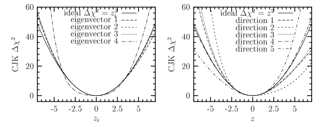
Figure 1: Left plot presents comparison of the $\chi^{2}$ dependence along each of four eigenvector directions to the ideal $\Delta\chi^{2}=z_{i}^{2}$ curve. In right plot analogous comparison for 5 random directions in $\{z_{i}\}$ space are shown. The ideal curve corresponds to $\Delta\chi^{2}=\sum z_{i}^{2}=z^{2}$

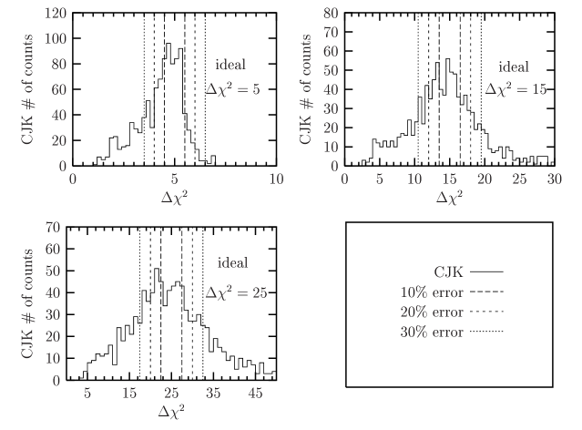
Figure 2: Test of the frequency distribution of $\Delta\chi^{2}$ for 1000 randomly chosen directions in the ${z_{i}}$ space normalized so that they correspond to the ideal $\Delta\chi^{2}=5,15$ or 25. The 10, 20 and 30% deviations from the expected $\Delta\chi^{2}$ are indicated in each plot.

In the left plot of Fig. 1 we present the comparison of the $\chi^{2}$ dependence along each of four eigenvector directions ($z_{i}=\delta_{ik}$ for the eigenvector $k$) to the ideal $\Delta\chi^{2}=z_{i}^{2}$ curve. We see again that only the line corresponding to the eigenvector 4 does not agree with the theoretical prediction. Moreover it has a different shape than other lines which results from the scaling adjustment procedure. In the right plot of Fig. 1 analogous comparison for the 5 randomly chosen directions in the $\{z_{i}\}$ space is shown. For each of directions $\sum_{k=1}^{4}z_{k}^{2}=z^{2}$ and the ideal curve corresponds to $\Delta\chi^{2}=z^{2}$. In this case we observe greater deviation from the quadratic approximation. Finally we test the frequency distribution of $\Delta\chi^{2}$ for randomly chosen directions in the $\{z_{i}\}$ space. Figure 2 presents the frequency distribution for 1000 $\{z_{i}\}$ directions normalized in such a way that they correspond to the ideal $\Delta\chi^{2}=5,15$ or 25 ($z=\sqrt{5},\sqrt{15}$ or 5 respectively). The 10, 20 and 30% deviations from the theoretical $\Delta\chi^{2}$ are indicated in each plot. We observe that, as could be expected, the quadratic approximation worsens with increasing $z$. Still the central peak is well outlined even in the last histogram. Fractions of the counts within the successive lines of the increasing deviation from the theoretical predictions are given in table 5. Even for high $\Delta\chi^{2}=25$ more than half of the counts are contained in the 30% error range.

	10%	20%	30%
$\Delta\chi^{2}=5$	0.477	0.652	0.792
$\Delta\chi^{2}=15$	0.266	0.498	0.667
$\Delta\chi^{2}=25$	0.251	0.401	0.586

Table 5: Fractions of the counts within the successive lines of the increasing deviation from the ideal $\Delta\chi^{2}$ for 1000 randomly chosen directions in the $\{z_{i}\}$ space (see text and figure 2) for the CJK model.

3.4 Collection of test CJK parametrizations

After checking that the Hessian method gives reasonable results for the case of our CJK model we can create a collection of test parametrizations of the parton densities, $\{S_{i}^{\pm}\}$, for that model. We only need to choose the value of the magnitude $t$ of equations (16) and (17). We performed tests with $t=1,\sqrt{5},\sqrt{10}$ and 5 and noticed hardly any dependence of the uncertainties of parton densities or example physical cross-sections on its choice. We decided to apply $t=5$. That way the $\{S_{i}^{\pm}\}$ collection of eight parametrizations containing information about the CJK fit uncertainties was created. All sets of parameters are presented in table 6.

eigenvector	Set		$\kappa$	$\alpha$	$\beta$	$N_{v}$
1	Set $1^{+}$		1.916	0.344	0.893	0.377
	Set $1^{-}$		1.952	0.258	0.903	0.430
2	Set $2^{+}$		1.937	0.378	0.841	0.544
	Set $2^{-}$		1.932	0.224	0.952	0.271
3	Set $3^{+}$		2.462	0.480	0.975	0.323
	Set $3^{-}$		1.437	0.129	0.826	0.481
4	Set $4^{+}$		1.754	0.525	1.912	0.691
	Set $4^{-}$		2.072	0.127	0.124	0.185

Table 6: Parameters of the collection of CJK parametrizations.

Next, in table 7 we present again the parameters of the CJK model with their errors calculated within the Hessian quadratic approximation for the standard requirement of $\Delta\chi^{2}=1$. These uncertainties should be compared with the errors calculated by Minuit and shown in table 1. They are of the same order but slightly smaller. Note that the uncertainties given in table 7 can be simply multiplied by the tolerance parameter $T$ to obtain errors which would correspond to an assumption of a higher $\Delta\chi^{2}$ value (see Eq. 18).

model		$\kappa$	$\alpha$	$\beta$	$N_{v}$
CJK		$1.934^{+0.112}_{-0.103}$	$0.299^{+0.061}_{-0.051}$	$0.898^{+0.204}_{-0.156}$	$0.404^{+0.066}_{-0.054}$

Table 7: The parameters of the fits for CJK model with errors calculated in the Hessian quadratic approximation for the standard requirement of $\Delta\chi^{2}=1$

All test parton distributions along with $F_{2}^{\gamma}(x,Q^{2})$ are further parametrized on the grid. The resulting FORTRAN program can be found on the web-page [27].

3.5 Uncertainties of the CJK parton densities

In this section we discuss the uncertainties of the CJK model parton densities.

In Figures 3–7 the quark and gluon densities calculated in FFNS_CJK models and GRV LO [29], GRS LO [10] and SaS1D [11] parametrizations are compared with the CJK predictions. We plot for $Q^{2}=10$ and 100 GeV² the $q^{\gamma}(\mathrm{Other\>model})/q^{\gamma}(\mathrm{CJK})$ and
$q^{\gamma}(\mathrm{Other\>parametrization})/q^{\gamma}(\mathrm{CJK})$ ratios of the parton $q^{\gamma}$ densities calculated in the CJK model and their values obtained with other models and parametrizations. Solid lines show the CJK fit uncertainties for $\Delta\chi^{2}=25$ computed with the $\{S_{i}^{\pm}\}$ test parametrizations.

First we notice that there is only one range of $x$, namely $0.01^{<}\hskip-7.11317pt_{\sim}x^{<}\hskip-7.11317pt_{\sim}0.1$ at $Q^{2}=10$ GeV² where the up- and down-quark densities predicted by the FFNS_CJK 1 fit go slightly beyond the uncertainty bands. Apart from that the predictions of FFNS_CJK models in the case of all parton distributions lie between the lines of the CJK uncertainties. That indicates that the choice of $\Delta\chi^{2}=25$ agrees with the differences among our three models. Moreover the GRV LO parametrization predictions are nearly contained within the CJK model uncertainties. That is not the case only for the heavy-quark densities. To hold the GRS LO and SaS1D parametrization curves in that range would require a much increased $\Delta\chi^{2}$ value. Especially the SaS1D results differ very substantially from the CJK ones.

We observe that the up-quark distribution is the one best constrained by the experimental data. As could be expected the greatest uncertainties are connected with the gluon densities. In the case of $u^{\gamma}$ the $\Delta\chi^{2}=25$ band widens in the small $x$ region. Alike in the case of other quark uncertainties it shrinks at high-$x$. On contrary the gluon distributions are least constrained at the region of $x\to 1$. That results from the fact that the gluon density contributes to $F_{2}^{\gamma}(x,Q^{2})$ mainly through the $\gamma^{*}G\to q\bar{q}$ process which gives numerically important results only at small-x and therefore only in that region experimental data can constrain it. Finally we see that all uncertainties become slightly smaller when we go to higher $Q^{2}$ from 10 to 100 GeV².

4 Lagrange method for the uncertainties of the parton distributions

The Hessian method, discussed above, is a very useful tool as it allows for computing of the parton density uncertainties in a very simple and effective way. If we find that our $\Delta\chi^{2}$ was assumed too rigorously or on contrary too conservatively we can obtain the uncertainties corresponding to any other $\Delta\chi^{2}$ value by simple scaling of the previous results. Still, the Hessian method relies on the assumption of the quadratic approximation, which in the case of our analysis is not perfectly preserved. Therefore, it is very important to perform a cross-check of the obtained results by comparing them to the corresponding results derived in a different statistical approach.

There exist another method called the Lagrange multiplier method (the Lagrange method in short) which allows to find exact uncertainties independently of the quadratic approximation. This method has also been applied to the proton structure case by the CTEQ Collaboration [5], [9] and the MRST group [8]. Here we utilize it to perform tests of the reliability of the Hessian approach results in the case of the CJK parton distributions.

In the Lagrange method we make a series of fits on the quantity

$$F(\lambda,\{a_{i}\})=\chi^{2}(\{a_{i}\})+\lambda X(\{a_{i}\}),$$ (19)

each with a different but fixed value of the Lagrange multiplier $\lambda$. As a result we obtain a set of points $(\chi^{2}(\lambda),X(\lambda))$ which characterize the deviation of the physical quantity $X$ from its best value $X_{0}$ for a corresponding deviation of the structure function global fit from its minimum $\Delta\chi^{2}=\chi^{2}(\lambda)-\chi_{0}$. In each of these constrained (by the $\lambda$ parameter) fits we find the best value of $X$ and the optimal $\chi^{2}$. For $\lambda=0$ we return to the basic structure function fit which gave us $\{a_{i}^{0}\}$ parameters and allowed to calculate the best $X_{0}$ value. The great advantage of this approach lies in the fact that we do not assume anything about the uncertainties. There is neither the quadratic nor any other approximation in that case. The large computer time consuming of the process of the whole series of minimalizations is its huge disadvantage.

5 Examples of cross-section uncertainties in Hessian and Lagrange methods

As was already said the Lagrange multiplier approach is a method on which we can rely whether the assumption of quadratic approximation of the Hessian is fulfilled or not. Unfortunately the amount of necessary computer calculations makes this approach very impractical. Still it can serve us as a final check of the correctness of the uncertainties that can be obtained using collections of our $\{S_{i}^{\pm}\}$ parametrizations calculated with the Hessian method. We will show a comparison of the uncertainties obtained in Hessian and Lagrange multiplier methods calculated with the CJK parton distributions for two physical quantities. First, for the one of $F^{\gamma}_{2,c}$ points measured by the OPAL Collaboration [30], as described in Section 4.3. Secondly, for the $\gamma q\to\gamma q$ part of the $\gamma\gamma$ prompt photon production cross-section.

5.1 $F^{\gamma}_{2,c}$

We chose to exam our collection of test parametrizations first on a very simple example of $F^{\gamma}_{2,c}$. The charm-quark structure function depends only on the charm-quark and gluon distributions which (especially the gluon density) are not well constrained by the experimental data. On the other hand this dependence is not very strong in the high-$x$ region where the direct Bethe-Heitler contribution dominates. Still we expect considerable deviation of the Hessian method results from the correct Lagrange approach predictions.

The [30] OPAL analysis provided the averaged $F^{\gamma}_{2,c}/\alpha$ values in two $x$ bins. For our purpose we chose the high-$x$ point at $x=0.2$ and $Q^{2}=20$ GeV². We calculate the CJK model prediction for $F^{\gamma}_{2,c}/\alpha$ and its Hessian uncertainties. Further we apply the Lagrange method with $\lambda=\pm 0.33,0.66,1,\cdots\times 10000$. The results are presented in Fig. 8. The solid line and crosses show the Hessian and Lagrange method predictions respectively. The dashed lines represent the 10 to 30% deviation from the Hessian results. As can be seen the Hessian method reproduces very well the Lagrange predictions in the direction of decreasing $F^{\gamma}_{2,c}$ even for $\Delta\chi^{2}$ greater than 100. On the other hand the agreement in the other direction corresponding to negative $\lambda$ is much worse. The lack of higher $\chi^{2}$ Lagrange points results from the negative $N_{v}$ parameter values appearing in the fits for $\lambda>1\times 10000$.

5.2 Prompt photon production

As the second example physical process we took a part of the prompt photon $\gamma\gamma$ production. Namely, for the sake of the limitation of the necessary computer time, we decided to calculate the direct resolved (DR) $\gamma q\to\gamma q$ cross-section. Any cross-section of two photons can be divided into three parts. The direct part which is a simple $\gamma\gamma$ electromagnetic interaction, the DR being the part in which one photon interacts with the partons originating from the second $\gamma$ and finally the doubly resolved (or resolved resolved, RR) part in which both photons interact through their hadronic structure. Only the resolved processes contribute to the prompt photon production. Unfortunately calculation of the RR part is very computer time consuming. Therefore as we are not interested in the quantitative result of our computation but we use it only to compare the uncertainties obtained in two methods we omit the doubly resolved contribution to the cross-section. The $\gamma q\to\gamma q$ process depends only on the quark distributions. We include the heavy-quark contributions with omitting their masses in calculations (the difference to the massive computation is on a 1% level). We calculate the cross-section for the photon beams energy $E_{\gamma}=200$ GeV. That can correspond to the high energy peak of the TESLA Photon Collider [31] built on the Linear Collider of the $e^{+}e^{-}$ central mass energy of 500 GeV.

The Lagrange method was applied with $\lambda=\pm 0.2,0.4,0.6,\cdots\times 1000$. The results of the comparison are presented in Fig. 9. Again the solid line and crosses show the Hessian and Lagrange method predictions respectively. The dashed lines represent the 10 to 30% deviation from the Hessian results. As we observe both methods agree very well in both directions of the change of the cross-section and in the whole range of the $\Delta\chi^{2}$ plotted.

6 $\chi^{2}$ of the CJK fit and the data

The CJK model presented in this article is, as described in detail in [1], a result of an improved analysis of [2] where our first CJKL model was given. Though we obtain a much better $\chi^{2}/_{\rm DOF}$ in the case of the CJK global fit to $F_{2}^{\gamma}(x,Q^{2})$ comparing to the previous CJKL fit, its value, 1.537, is large. Moreover, part of the improvement of the value of $\chi^{2}/_{\rm DOF}$ is due to the exclusion of the TPC2_γ data from the full set of the experimental $F_{2}^{\gamma}(x,Q^{2})$ results. Recently a similar global fit has been performed and presented in [26] for the case of the simple FFNS type model with the Bethe-Heitler process describing the heavy-quark contributions. The result of that fit is $\chi^{2}/_{\rm DOF}=0.938$. The authors applied 134 $F_{2}^{\gamma}(x,Q^{2})$ points. In this section we try to indicate the main sources of the large $\chi^{2}/_{\rm DOF}$ of our CJK fit to 182 data points. We also try to judge whether any exclusions of the data from the fits can be justified.

We performed a few simple tests. First, for the case of the additional test global fit containing the full set of the available data, mentioned in section 3.2 and denoted further as FULL. We calculated the $\chi^{2}_{n}/N_{n}$ for each of the data collections as explained in 3.2. The $\chi^{2}_{n}$, being the value of the $\chi^{2}$ of the best fit corresponding to the given experiment, divided by the number of the experimental points $N_{n}$ shows the agreement of each of the data collections with the global fit. Results are presented in the table 8. Obviously, as different sets of the data were applied in this and CJK fits the corresponding numbers in tables 2 and 8 are not the same. The FULL fit results show that the global test similarly disagree with three of the data sets, the TPC2_γ, DESY and DELPHI.

Set		TPC2γ	DESY	KEK	ALEPH	DELPHI	L3	OPAL
$\chi^{2}_{n}/N_{n}$		2.38	2.44	1.20	1.07	2.25	0.60	0.97

Table 8: The $\chi^{2}_{n}$, being the value of the $\chi^{2}$ of the best fit corresponding to the given experiment, divided by the number of the experimental points $N_{n}$ for the case of the test global FULL fit to the full set of the available data.

Secondly, we calculated the contribution to the $\chi^{2}$ of the FULL fit given by each of the 208 data points. We performed the same computation for the GRS [10] and SaS1D [11] parametrizations as well as for the two FFNS_CJK fits presented in [1] (obtained without the TPC2_γ data). We found the data which contribution to the $\chi^{2}$ in case of each of the mentioned fits is larger than 3. It appeared that there are 5 such points among 12 in the case of the CELLO experiment, [13], belonging to the DESY collection. Moreover, there are 9 such points among 22 in the case of the DELPHI’01 experiment, [20], belonging to the DELPHI collection. On the other hand we found only 2 such points in the case of the TPC2_γ data. In other experiments there are no more than single cases of that kind.

As the DESY and DELPHI sets are the collections of various measurements (in the DELPHI experiment case they differ by the year of publication) we checked in more detail the $\chi^{2}_{n}/N_{n}$ for each of those measurements in the case of the FULL fit. The results, presented in the table 9, confirm that as could be expected from the above test the CELLO and DELPHI’01 results give main contributions to the high $\chi^{2}_{n}/N_{n}$ of the DESY and DELPHI collections respectively.

Set		PLUTO	JADE	CELLO	TASSO	DELPHI’96	DELPHI’98	DELPHI’01
$\chi^{2}_{n}/N_{n}$		0.64	1.12	5.88	1.01	1.04	0.10	3.65

Table 9: The $\chi^{2}_{n}$, being the value of the $\chi^{2}$ of the best fit corresponding to the given experiment, divided by the number of the experimental points $N_{n}$ for the case of the global FULL fit to the full set of the available data.

Further, we performed another five test fits of the CJK model to the full data set from which we excluded the CELLO, DELPHI’01 and finally pairs of CELLO, DELPHI’01 and TPC2_γ measurements. We denote those fits as NOCEL, NODEL (CJK fit = NOTPC) and NOTPCCEL, NOTPCDEL, NOCELDEL respectively. The $\chi^{2}$, the number of experimental points and $\chi^{2}/_{\rm DOF}$ for the CJK and each of the six test fits are presented in table 10. The FULL fit including all available data has highest $\chi^{2}/_{\rm DOF}$ value. The exclusion of the TPC2_γ measurement, proposed in [26], improves it but not very much, see the CJK fit result. The NOCEL and NODEL fits give much better agreement between the model and the data but still in their case $\chi^{2}/_{\rm DOF}$ is larger than 1. We see that only exclusion of two of the CELLO, DELPHI’01 and TPC2_γ measurements at the same time leads to the $\chi^{2}/_{\rm DOF}\approx 1$. Finally, we notice that the best $\chi^{2}/_{\rm DOF}$ is obtained in the case of the NOCELDEL fit. Central values of the parameters calculated in the additional test fits (not shown) and of the CJK fit (given in table 1) lie inside the sum of their uncertainties. This statement is true for both cases of the CJK fit uncertainties: obtained from Minos (see table 1) and calculated in the Hessian quadratic approximation (see table 7). Only differences between the central values of the $\beta$ parameter are slightly larger than the sums of the corresponding uncertainties. Therefore, we examined the agreement among the parton distributions computed in the CJK model in each of the fits. Figure 10 presents the comparison of the six test fit results with the CJK parton densities and their uncertainties obtained in the Hessian method for $\Delta\chi^{2}=25$ and $Q^{2}=10$ GeV². We notice that the test distributions are in agreement with the CJK densities in the sense that they are contained within the CJK uncertainties for the assumed allowed deviation of the global fit from the minimum. Especially, we observe a very small difference among the CJK, FULL, NOCEL and NOTPCCEL parton distributions. The only deviation is observed in the case of the up- and down-quark densities at high-$x$ computed for the NODEL and NOTPCDEL fits. The results at other $Q^{2}$ values are very similar.

FIT		FULL		CJK	NOCEL	NODEL		NOTPCCEL	NOTPCDEL	NOCELDEL
$\chi^{2}$		338.7		273.7	262.4	244.0		200.7	169.4	179.5
points		208		182	196	186		170	160	174
$\chi^{2}/_{\rm DOF}$		1.66		1.54	1.37	1.34		1.21	1.08	1.06

Table 10: The $\chi^{2}$, the number of experimental points and $\chi^{2}/_{\rm DOF}$ for CJK fit and six additional test fits. Fit denoted as FULL contains all the available data. The NOCEL, NODEL and CJK fits exclude the CELLO [13], DELPHI’01 [20] and TPC2_γ [25] measurements respectively. The NOTPCCEL, NOTPCDEL and NOCELDEL fits exclude pairs of CELLO, DELPHI’01 and TPC2_γ data.

We notice that the value of $\chi^{2}/_{\rm DOF}$ for the global fits of our CJK model depends very strongly on the choice of the data set applied in the fit, on the other hand, they produce similar parton distributions which lie within the CJK parton density uncertainties. Especially, as was noticed, the parton distributions predicted by our CJK and by the FULL fit, including all available $F_{2}^{\gamma}(x,Q^{2})$ data, differ very slightly.

7 Summary

The very first analysis of the uncertainties of the radiatively generated parton distributions in the real photon based on the LO DGLAP equations is given. We consider the CJK model presented in [1]. The estimate of the uncertainties of the CJK parton densities due to the experimental errors is based on the Hessian method which was recently applied in the proton parton structure analysis. We test the applicability of the approach by comparing uncertainties of example cross-sections calculated in the Hessian and Lagrange methods. Sets of test parametrizations are given, which allow for calculation of its best fit parton distributions along with $F_{2}^{\gamma}(x,Q^{2})$ and for computation of uncertainties of any physical value depending on the real photon parton densities. Finally, we present a detailed analysis of the $\chi^{2}$ of the CJK fit and its relation to the data. We show that large $\chi^{2}/_{\rm DOF}$ of the fit is due to only a few of the experimental measurements. By excluding them $\chi^{2}/_{\rm DOF}\approx 1$ can be obtained. A FORTRAN program with the grid parametrization of the test parton distributions and $F_{2}^{\gamma}(x,Q^{2})$ can be obtained from the web-page [27].

Our work is the first trial to estimate the uncertainties of the real photon parton distributions. Future analysis of that kind should include the corrections taking into account all possible sources of the deviation of the experimental $F_{2}^{\gamma}(x,Q^{2})$ data from the photon structure function as described by the theoretical models.

Figure 3: Up-quark densities calculated in FFNS_CJK models and GRV LO [29], GRS LO [10] and SaS1D [11] parametrizations compared with the CJK predictions. We plot for $Q^{2}=10$ and 100 GeV² the $u^{\gamma}(\mathrm{Other\>model})/u^{\gamma}(\mathrm{CJK})$ and $u^{\gamma}(\mathrm{Other\>parametrization})/u^{\gamma}(\mathrm{CJK})$ ratios of the up-quark density calculated in the CJK model and its values obtained with other models and parametrizations. Solid lines show the CJK fit uncertainties for $\Delta\chi^{2}=25$ computed with the set of $\{S_{i}^{\pm}\}$ test parametrizations.

Figure 4: The same as in Fig. 3, for the down quark.

Figure 5: The same as in Fig. 3, for the strange quark.

Figure 6: The same as in Fig. 3, for gluon.

Figure 7: The same as in Fig. 3, for the charm and beauty quark. Only parametrizations including heavy-quark distributions are compared with the CJK model predictions.

Figure 8: The comparison of the Lagrange and Hessian method results for the high bin $F^{\gamma}_{2,c}$ of the OPAL [30] meauserement. The solid line and crosses show the Hessian and Lagrange method predictions respectively. The dashed lines represent the 10 to 30% deviation from the Hessian result.

Figure 9: The comparison of the Lagrange and Hessian method results for the direct resolved (DR) part of the $\gamma\gamma\to\gamma q$ cross-section. The solid line and crosses show the Hessian and Lagrange method predictions respectively. The dashed lines represent the 10 to 30% deviation from the Hessian result.

Figure 10: Comparison of the test fit parton distributions with the CJK parton densities and their uncertainties. Fit denoted as FULL contains all the available data. The NOCEL, NODEL and CJK fits exclude the CELLO [13], DELPHI’01 [20] and TPC2_γ [25] measurements respectively. The NOTPCCEL, NOTPCDEL and NOCELDEL fits exclude pairs of CELLO, DELPHI’01 and TPC2_γ data. We plot for $Q^{2}=10$ GeV² the $q^{\gamma}(\mathrm{Other\>fits})/q^{\gamma}(\mathrm{CJK})$ ratios of densities calculated in the CJK fit and their values obtained in other fits. Solid lines show the CJK fit uncertainties for $\Delta\chi^{2}=25$ computed with the set of $\{S_{i}^{\pm}\}$ test parametrizations.

References

- [1] F.Cornet, P.Jankowski, M.Krawczyk, to be published in Proceedings of International Conference on the Structure and Interactions of the Photon and 15th International Workshop on Photon-Photon Collisions (Photon 2003), Frascati, Italy, 2003, hep-ph/0310029; F.Cornet, P.Jankowski, M.Krawczyk, IFT-2003-30
- [2] F.Cornet, P.Jankowski, M.Krawczyk and A.Lorca, Phys. Rev D68, 014010 (2003)
- [3] M.Glück, E.Reya and M.Stratmann, Phys. Rev. D51, 3220 (1995)
-
[4]
S.Kretzer, C.Schmidt and W.Tung,
Proceedings of New Trends in HERA Physics,
Ringberg Castle, Tegernsee, Germany, 17-22
Jun 2001, Published in J. Phys. G28, 983 (2002);
S. Kretzer, H.L. Lai, F.I. Olness and W.K. Tung, hep-ph/0307022 - [5] J.Pumplin, D.R.Stump and W.K.Tung, Phys. Rev. D65, 014011 (2002)
- [6] J.Pumplin et al., Phys. Rev. D65, 014013 (2002)
- [7] J.Pumplin et al., JHEP 0207, 012 (2002)
- [8] A.D.Martin, R.G.Roberts, W.J.Stirling and R.S.Thorne, hep-ph/0211080
- [9] D.Stump et al., Phys. Rev. D65, 014012 (2002)
- [10] M.Glück, E.Reya and I.Schienbein, Phys. Rev. D60, 054019 (1999), Erratum-ibid. D62, 019902 (2000)
- [11] G.A.Schuler and T.Sjöstrand, Z. Phys. C68, 607 (1995); Phys. Lett. B376, 193 (1996)
- [12] J.H.Field, VIIIth International Workshop on Photon-Photon Collisions, Shoresh, Jerusalem Hills Israel, 1988; U. Maor, Acta Phys. Polonica B19, 623 (1988); Ch. Berger and W. Wagner, Phys. Rep. 146, 1 (1987)
- [13] CELLO Collaboration, H. J. Behrend et al., Phys. Lett. B126, 391 (1983); in Proceedings of the XXVth International Conference on High Energy Physics, Singapore, 1990, edited by K. K. Phua and Y. Yamaguchi (World Scientific, Singapore, 1991).
- [14] PLUTO Collaboration, Ch. Berger et al., Phys. Lett. B142 111 (1984); Nucl. Phys. B281, 365 (1987).
- [15] JADE Collaboration, W. Bartel et al., Z. Phys. C24, 231 (1984).
- [16] TASSO Collaboration, M. Althoff et al., Z. Phys. C31, 527 (1986).
- [17] TOPAZ Collaboration, K. Muramatsu et al., Phys. Lett. B332, 477 (1994).
- [18] AMY Collaboration, S. K. Sahu et al., Phys. Lett. B346, 208 (1995); T. Kojima et al., ibid. B400, 395 (1997).
- [19] DELPHI Collaboration, P. Abreu et al., Z. Phys. C69, 223 (1996); I. Tyapkin, in Proceedings of Workshop on Photon Interaction and the Photon Structure, Lund, Sweden, 1998, edited by G. Jarlskog and T. Sjöstrand,
- [20] I. Tyapkin, in Proceedings of International Conference on the Structure and Interactions of the Photon and 14th International Workshop on Photon-Photon Collisions (Photon 2001), Ascona, Switzerland, 2001.
- [21] L3 Collaboration, M. Acciarri et al., Phys. Lett. B436, 403 (1998); ibid. B447, 147 (1999); ibid. B483, 373 (2000).
- [22] ALEPH Collaboration, R. Barate et al., Phys. Lett. B458, 152 (1999); K. Affholderbach et al., Proceedings of the International Europhysics Conference on High Energy Physics, Tampere, Finland, 1999, Nucl. Phys. Proc. Suppl. B86, 122 (2000).
- [23] OPAL Collaboration, K. Ackerstaff et al., Z. Phys. C74, 33 (1997); Phys. Lett. B411, 387 (1997); G. Abbiendi et al., Eur. Phys. J. C18, 15 (2000).
- [24] OPAL Collaboration, G. Abbiendi et al., Phys. Lett. B533, 207 (2002).
- [25] TPC/ Collaboration, H. Aihara et al., Z. Phys. C34, 1 (1987); J. S. Steinman, Ph.D. Thesis, UCLA-HEP-88-004, Jul 1988.
- [26] S. Albino, M. Klasen and S. Söldner-Rembold, Phys. Rev. Lett. 89, 122004 (2002).
-
[27]
http://www.fuw.edu.pl/
~pjank/param.html - [28] F.James and M.Roos, Comput. Phys. Commun. 10, 343 (1975)
- [29] M.Glück, E.Reya and A.Vogt, Phys. Rev. D46, 1973 (1992)
- [30] OPAL Collaboration, G.Abbiendi et al., Phys. Lett. B539, 13 (2002)
- [31] TESLA Technical Design Report. Part 6. Appendices. Chapter 1. “Photon Collider at TESLA.” (B. Badelek et al.). DESY-01-011, hep-ex/0108012