Precision Electroweak Observables in the Minimal Moose Little Higgs Model

Abstract:

Little Higgs theories, in which the Higgs particle is realized as the pseudo-Goldstone boson of an approximate global chiral symmetry have generated much interest as possible alternatives to weak scale supersymmetry. In this paper we analyze precision electroweak observables in the Minimal Moose model and find that in order to be consistent with current experimental bounds, the gauge structure of this theory needs to be modified. We then look for viable regions of parameter space in the modified theory by calculating the various contributions to the S and T parameters.

1 Introduction

Despite its spectacular agreement with current experimental data, the Standard Model (SM) is widely held to be incomplete due to an instability in its Higgs sector; radiative corrections to the Higgs mass suffer from one-loop quadratic divergences leading to an undesirable level of fine-tuning between the bare mass and quantum corrections. This suggests the emergence of new physics at energy scales around a TeV, which will be investigated in the near future with direct accelerator searches. The electroweak sector of the SM has been probed to better than the 1% level by precision experiments at low energies as well as at the $Z$-pole by LEP and SLC. The data obtained can also severely constrain possible extensions of the SM at TeV energies [1, 2, 3, 4].

Recently, a new class of theories known as Little Higgs (LH) models [5, 6, 7, 8, 9, 10, 11] have been proposed to understand the lightness of the Higgs by making it a pseudo-Goldstone boson. Approximate global symmetries ensure the cancellation of all quadratic sensitivity to the cutoff at one loop in the gauge, Yukawa and Higgs sectors, by partners of the same quantum statistics: heavy gauge bosons cancel the divergence of the SM gauge loop; massive scalars do the same for the Higgs self-coupling, as do heavy fermions for the top loop contributions. These partner particles have masses of the order of the symetry breaking scale $f$, which we take to be a few TeV. At lower energies the presence of these new particles can be felt only through virtual exchanges and and their effects on precision electroweak oberservables (PEWOs).

In this paper we calculate corrections to PEWOs in the Minimal Moose (MM) [5], and in a similar model with a slight variation in gauge structure (the Modified Minimal Moose, or MMM) in an attempt to find regions of parameter space where these are small with a tolerable level of fine tuning in the Higgs sector.

Both models have a simple product gauge structure $G_{L}\times G_{R}$ and reduce to the SM with additional Higgs doublets at low energies. Above the symmetry breaking scale the Higgs sector is a nonlinear sigma model which becomes strongly coupled at $\Lambda\simeq 10$ TeV and requires UV completion at higher energies. The enhanced gauge sector can contribute to precision observables through the interaction of the partners to SM gauge bosons, $W^{\prime}$ and $B^{\prime}$, with fermions and Higgs doublets via currents $j^{\mu}_{F}$ and $j^{\mu}_{H}$ respectively, generating low energy operators of the form $j_{F}j_{F}$, $j_{F}j_{H}$ and $j_{H}j_{H}$. We group these into oblique and non-oblique corrections, where the former impact precision experiments only via their effects on gauge boson propagators, and summarize their salient properties below.

Oblique corrections can originate from:

• Interactions $j_{H}j_{H}$
  $B^{\prime}$ exchange modifies the $Z_{0}$ mass and hence introduces custodial $SU(2)$ violating effects to which the $T$ parameter is sensitive. This is a cause for concern in the MM, but is reduced considerably in the Modified Moose by gauging a different subset of the global symmetries.

• Non-linear sigma model (nlsm) kinetic terms
  At energies above the global symmetry breaking scale, the Higgs doublets form components of nlsm fields with self-interactions. This gives rise to custodial $SU(2)$ violating operators in the low energy theory which become our most significant constraint.

• Higgs-heavy scalar interactions
  The theories also contain a scalar potential in the form of plaquette terms to ensure that electroweak symmetry is broken appropriately. This contributes to the $T$ parameter through the exchange of heavy scalar modes, which effect we show to be negligible.

• Fermion loops
  The presence of a vector-like partner to the top quark is another source for $T$ and $S$ parameter contributions. We calculate these and show that they are tolerably small for a wide range of parameters of the theory.

• Higgs loops
  Since the MM is a two Higgs doublet theory at low energies, corrections due Higgs loops are similar to those of the Minimal Supersymmetric Standard Model.

The following are the non-oblique corrections of concern to us:

• Four-fermion operators $j_{F}j_{F}$
  These modify $G_{F}$ and can be controlled in the MMM in the near-oblique limit (see below), in which light SM fermions decouple from the $W^{\prime}$ and $B^{\prime}$.

• Interactions $j_{F}j_{H}$
  Operators of this form shift the coupling of the SM gauge bosons to the fermions (most easily seen in unitary gauge). These are also minimized in the near-oblique limit.

LH gauge sectors generically have a simple limit in which highly constrained non-oblique corrections vanish (the near-oblique limit [7]) in tandem with oblique corrections from the gauge boson sector. In the MM however, the $SU(3)\times SU(2)\times U(1)$ gauge structure is too tightly constrained to allow for a decrease in the large oblique $B^{\prime}$ correction by variation of the gauge couplings. This issue is resolved in the MMM by replacing the $SU(3)$ gauge group by another $SU(2)\times U(1)$ and charging the light fermions equally under both $U(1)$s, giving

$$j_{H},j_{F_{light}}\propto\tan{\theta^{\prime}}-\cot{\theta^{\prime}}$$

for $\tan{\theta^{\prime}}=g_{1R}/g_{1L}$, the ratio of the U(1) couplings at the sites. Setting these nearly equal to each other rids us of large heavy gauge boson contributions to the $T$ parameter as well as undesirable light four-fermion operators arising from $B^{\prime}$ exchange. This method does not work with third-generation fermions which are coupled to the Higgs in a slightly different way. Possible non-oblique corrections involving these will not be discussed since they are not yet unambiguously constrained by experiment. For additional discussion of this see [7]. $W^{\prime}$- exchange operators are more easily handled since, provided we stay away from the strong coupling regime, increasing one of the SU(2) gauge couplings with respect to the other increases the mass of the $W^{\prime}$, effectively decoupling it from our theory.

We begin this paper with a brief review of the MM, keeping as far as possible to the conventions used in [5]. In Sections 3 to 5 we calculate tree-level corrections to PEWOs from different sectors. We go on to discuss electroweak symmetry breaking in the low energy theory (Section 6) and determine loop effects due to a new heavy fermion (Section 7) and Higgs doublets (Section 8). In spite of the fact that the MM is inconsistent with current constraints on PEWOs we show in Section 9 that there are regions in the parameter space of the MMM where all except third generation non-oblique corrections can be eliminated, with tolerably small oblique corrections. We will see that the most unforgiving aspect of both models is the non-linear sigma model sector which has no residual $SU(2)_{c}$ symmetry and hence gives rise to a $T$ parameter contribution that can only be decreased by adjusting $f$. This compels us to choose $f\gtrsim 2$ TeV. We display two sets of parameters, one that is well within the 1.5-$\sigma$ $S$-$T$ ellipse with a 17% fine tuning in the SM Higgs mass and another that falls just outside the ellipse with a 3% fine tuning. We show that there are regions of parameter space where one can do even better than the first set, however this is only possible for a rather specific choice of parameters. We measure fine tuning by $(m/\delta m)^{2}$, where $\delta m$ is the top loop correction to the mass of the Higgs doublet, and $m$ is the physical Higgs mass.

2 The Theory

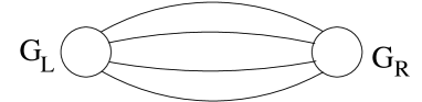
Figure 1: The Minimal Moose

The Minimal Moose is a two-site four-link model with gauge symmetry $G_{R}=SU(3)$ at one site and $G_{L}=SU(2)\times U(1)$ at the other. The standard model fermions are charged under $G_{L}$, with their usual quantum numbers while the link fields $X_{j}=\exp(2ix_{j}/f)$ are 3 by 3 nonlinear sigma model fields transforming as bifundamentals under $G_{L}\times G_{R}$ where a fundamental of $G_{L}$ is $\textbf{2}_{1/6}\oplus\textbf{1}_{-1/3}$. These fields get strongly coupled at a scale $\Lambda=4\pi f$, beneath which the theory is described by the Lagrangian

$$\mathcal{L}=\mathcal{L}_{G}+\mathcal{L}_{\chi}+\mathcal{L}_{t}+\mathcal{L}_{\psi}$$ (1)

$\mathcal{L}_{G}$ includes all kinetic terms and gauge interactions, while $\mathcal{L}_{\chi}$ contains plaquette couplings between the $X_{j}$:

$$\mathcal{L}_{\chi}=\left(\frac{f}{2}\right)^{4}\bigg{(}\text{\,Tr\,}\left[A_{1}X_{1}X_{2}^{{\dagger}}X_{3}X_{4}^{{\dagger}}\right]+\text{\,Tr\,}\left[A_{2}X_{2}X_{3}^{{\dagger}}X_{4}X_{1}^{{\dagger}}\right]$$

$$+\text{\,Tr\,}\left[A_{3}X_{3}X_{4}^{{\dagger}}X_{1}X_{2}^{{\dagger}}\right]+\text{\,Tr\,}\left[A_{4}X_{4}X_{1}^{{\dagger}}X_{2}X_{3}^{{\dagger}}\right]\bigg{)}+\mathrm{h.c.}$$ (2)

with $A_{i}=\kappa_{i}+\epsilon_{i}T^{8}$ for $\epsilon\sim\kappa/10$. This is a natural relation since any radiative corrections to $\epsilon$ require spurions from both the gauge and plaquette sectors and so can only arise at two loops. The $\epsilon$ terms give the little Higgses a mass (see Equation 30) and are required to stabilize electroweak symmetry breaking (EWSB).

The third generation quark doublet is coupled to a pair of colored Weyl fermions $U$,$U^{c}$ via Yukawa terms in $\mathcal{L}_{t}$

$$\mathcal{L}_{t}=\lambda f\left(\begin{array}[]{ccc}0&0&u_{3}^{c^{\prime}}\end{array}\right)X_{1}X_{4}^{{\dagger}}\left(\begin{array}[]{c}q_{3}\\ U\end{array}\right)+\lambda^{{}^{\prime}}fUU^{c}+\text{ h.c}$$ (3)

and $\mathcal{L}_{\psi}$ contains the remaining Yukawa couplings. These take the same form as above for the light up-type quarks, but with $U$ and $U^{c}$ removed, while the down and charged lepton sectors look like

$$\mathcal{L}_{\psi}\supset\lambda_{D}\left(\begin{array}[]{cc}q&0\end{array}\right)X_{1}X_{4}^{{\dagger}}\left(\begin{array}[]{c}0\\ 0\\ d^{c}\end{array}\right)+\lambda_{E}\left(\begin{array}[]{cc}l&0\end{array}\right)X_{1}X_{4}^{{\dagger}}\left(\begin{array}[]{c}0\\ 0\\ e^{c}\end{array}\right)+\text{ h.c}$$ (4)

We also impose a $Z_{4}$ symmetry which cyclically permutes the link fields and hence requires equality of all the decay constants ($f_{i}=f$) and plaquette couplings ($\kappa_{i}=\kappa$, $\epsilon_{i}=\epsilon$). The only $Z_{4}$-breaking terms arise in the fermion sector and are small.

3 The Gauge Boson Sector

The link fields Higgs the $G_{L}\times G_{R}$ gauge groups down to the diagonal $SU(2)\times U(1)$ subgroup, leaving one set each of massive and massless gauge bosons. This can be seen explicitly by considering the link field covariant derivatives:

$$\widetilde{D}_{\mu}X_{j}=\partial_{\mu}X_{j}-ig_{3}X_{j}A_{\mathbf{3,R}\mu}^{A}\mathbf{T}^{A}+ig_{2}A_{\mathbf{2,L}\mu}^{a}\mathbf{T}^{a}X_{j}+iqg_{1}A_{\mathbf{1,L}\mu}\mathbf{T}^{8}X_{j}$$ (5)

where the $\mathbf{T}$s for $A=1,...,8$ and $a=1,2,3$ are $SU(3)$ generators normalized such that $\text{\,Tr\,}[\mathbf{T}^{A}\mathbf{T}^{B}]=\frac{\delta^{AB}}{2}$ (similarly for a,b indices); and $q=1/\sqrt{3}$ to ensure that the Higgs doublet eventually has the correct SM hypercharge. Expanding out the fields ($X_{j}=\exp(2ix_{j}/f)$) in the kinetic term

$$\frac{f^{2}}{4}\text{\,Tr\,}\left[\sum_{j=1}^{4}(\widetilde{D}_{\mu}X_{j})(\widetilde{D}^{\mu}X_{j})^{\dagger}\right]$$ (6)

shows that the eaten Goldstone boson, $w$, is proportional to $x_{1}+x_{2}+x_{3}+x_{4}$. Orthogonal combinations $x$,$y$ and $z$ can be defined as follows:

$$\left(\begin{array}[]{c}w\\ z\\ x\\ y\end{array}\right)=\frac{1}{2}\left(\begin{array}[]{cccc}+1&+1&+1&+1\\ +1&-1&+1&-1\\ -1&-1&+1&+1\\ -1&+1&+1&-1\end{array}\right)\\ \left(\begin{array}[]{c}x_{1}\\ x_{2}\\ x_{3}\\ x_{4}\end{array}\right)\\$$ (7)

where each of the above fields decomposes under $SU(2)\times U(1)$ as $\textbf{3}_{0}$ $(\phi)$ + $\textbf{1}_{0}$ $(\eta)+\textbf{2}_{\pm 1/2}$ $(h\text{ and }h^{{\dagger}}).$

$$x=\left(\begin{array}[]{cc}\widetilde{\phi}_{x}+\frac{\eta_{x}}{\sqrt{12}}&\frac{h_{x}}{\sqrt{2}}\\ \frac{h_{x}^{{\dagger}}}{\sqrt{2}}&\frac{-\eta_{x}}{\sqrt{3}}\end{array}\right)$$ (8)

The $x$ and $y$ contain two Higgs doublets in the more familiar form

$$h_{1}=\frac{h_{x}+ih_{y}}{\sqrt{2}}$$ (9)

$$h_{2}=\frac{h_{x}-ih_{y}}{\sqrt{2}}$$ (10)

and plaquette terms give $z$ a large tree level mass, so it can be integrated out of the theory at a TeV.

Going to unitary gauge results in a mass matrix for heavy gauge bosons $W^{\prime}_{\mu}$, $B^{\prime}_{\mu}$ and $A_{\mathbf{3}\mu}$ with eigenvalues $2gf/\sin{2\theta}$, $2qg^{\prime}f/\sin{2\theta^{\prime}}$ and $fg/\sin{\theta}$ respectively. The $W^{\prime}$ s and $B^{\prime}$ s are admixtures of $A_{\mathbf{3,R}}$, $A_{\mathbf{2,L}}$ and $A_{\mathbf{1,L}}$:

$$W_{\mu}^{a} = \cos{\theta}A_{\mathbf{2,L}\mu}^{a}+\sin{\theta}A_{\mathbf{3,R}\mu}^{a}$$

$$W^{\prime a}_{\mu} = -\sin{\theta}A_{\mathbf{2,L}\mu}^{a}+\cos{\theta}A_{\mathbf{3,R}\mu}^{a}$$

$$B_{\mu} = \cos{\theta^{\prime}}A_{\mathbf{1,L}\mu}+\sin{\theta^{\prime}}A_{\mathbf{3,R}\mu}^{8}$$ (11)

$$B^{\prime}_{\mu} = -\sin{\theta^{\prime}}A_{\mathbf{1,L}\mu}+\cos{\theta^{\prime}}A_{\mathbf{3,R}\mu}^{8}$$

with mixing angles defined as follows:

$$g = \frac{g_{2}g_{3}}{\sqrt{g_{2}^{2}+g_{3}^{2}}}\quad\quad\quad\quad\sin{\theta}=\frac{g}{g_{3}}$$

$$g^{\prime} = \frac{g_{1}g_{3}}{\sqrt{\left(qg_{1}\right)^{2}+g_{3}^{2}}}\quad\quad\sin{\theta^{\prime}}=\frac{qg^{\prime}}{g_{3}}$$

The Higgses couple to heavy gauge bosons via the following currents:

$$j^{a}_{W^{{}^{\prime}}\mu} = -\frac{ig}{2\tan{2\theta}}\left[h_{1}^{{\dagger}}\sigma^{a}\overleftrightarrow{D_{\mu}}h_{1}+h_{2}^{{\dagger}}\sigma^{a}\overleftrightarrow{D_{\mu}}h_{2}\right]$$

$$j_{B^{{}^{\prime}}\mu} = -\frac{\sqrt{3}iqg^{{}^{\prime}}}{2\tan{2\theta^{{}^{\prime}}}}\left[h_{1}^{{\dagger}}\overleftrightarrow{D_{\mu}}h_{1}+h_{2}^{{\dagger}}\overleftrightarrow{D_{\mu}}h_{2}\right]$$ (12)

where $D_{\mu}$ is a Standard Model covariant derivative and $\sigma$s are Pauli matrices.

Explicitly integrating out the heavy gauge bosons results in the following $SU(2)_{c}$ violating terms:

$$\frac{3}{16f^{2}}\cos{{}^{2}2\theta^{\prime}}\left[\left(h_{1}^{{\dagger}}D_{\mu}h_{1}\right)^{2}+\left(h_{2}^{{\dagger}}D_{\mu}h_{2}\right)^{2}+2\left(h_{1}^{{\dagger}}D_{\mu}h_{1}\right)\left(h_{2}^{{\dagger}}D^{\mu}h_{2}\right)\right]$$ (13)

$$+ \frac{1}{8f^{2}}\cos{{}^{2}2\theta}\left[\left(h_{1}^{{\dagger}}D_{\mu}h_{2}\right)\left(h_{2}^{{\dagger}}D^{\mu}h_{1}\right)-\left(h_{1}^{{\dagger}}D_{\mu}h_{1}\right)\left(h_{2}^{{\dagger}}D^{\mu}h_{2}\right)\right]+\mathrm{h.c.}$$

It seems surprising that there is a contribution from the heavy $W$ at all ($\cos^{2}{2\theta}$ term) since its coupling is custodial $SU(2)$-symmetric! The relevant operators appear with a relative minus sign, however, and cancel when we break electroweak symmetry, giving a total contribution to the $T$ parameter of $1.6\left(\frac{1\text{ TeV }}{f}\right)^{2}\cos^{2}{2\theta^{\prime}}$. This mechanism is responsible for some more fortuitous cancellation in the next section.

At first glance it seems like we can minimize the $B^{\prime}$ contribution to precision measurements by varying $\theta^{\prime}$. However we are constrained to $\sin{\theta^{\prime}}\lesssim 1/3$ by the relation

$$\tan{\theta_{W}}=\frac{1}{q}\frac{\sin{\theta^{\prime}}}{\sin{\theta}}$$

which gives us an unacceptably high $T$ parameter as well as large corrections to $G_{F}$ from $B^{\prime}$ exchange. To overcome this problem the MM can be modified by replacing the $SU(3)\times SU(2)\times U(1)$ gauge symmetry by $[SU(2)\times U(1)]^{2}$ whose generators can be embedded into $SU(3)$ as $\mathbf{T}^{1,2,3}$ and $\mathbf{T}^{8}$. This sidesteps the constraint, since we now have enough freedom to vary $\theta^{\prime}$ independently of $\theta$. If we charge the fermions under $G_{L}$ as before, we will still have to tolerate large non-oblique corrections. Altering the fermion couplings, however, by charging them under both U(1)s, gives a $B^{\prime}$- fermion coupling of:

$$ig^{\prime}\sum_{i}{\overline{f}_{i}\left(\frac{q_{L}}{\tan{\theta^{\prime}}}-q_{R}\tan{\theta^{\prime}}\right)\overline{\sigma}^{\mu}B^{\prime}_{\mu}f_{i}}$$ (14)

where $q_{L}$ and $q_{R}$ are the fermion charges under each of the U(1)s. We can set $q_{L}=q_{R}=q_{SM}/2$ for the light fermions to eliminate this coupling at $\theta^{\prime}\simeq\pi/4$, provided we adjust the light yukawa couplings to account for the new gauge structure:

$$\mathcal{L}_{up} = \left[\lambda_{U}\left(\begin{array}[]{ccc}0&0&u^{c}\end{array}\right)X_{1}X_{4}^{{\dagger}}\left(\begin{array}[]{c}q\\ 0\end{array}\right)\right][X_{33}]^{-\frac{3}{4}}+\text{ h.c}$$ (18)

$$\mathcal{L}_{down} = \left[\lambda_{D}\left(\begin{array}[]{cc}q&0\end{array}\right)X_{1}X_{4}^{{\dagger}}\left(\begin{array}[]{c}0\\ 0\\ d^{c}\end{array}\right)+\lambda_{E}\left(\begin{array}[]{cc}l&0\end{array}\right)X_{1}X_{4}^{{\dagger}}\left(\begin{array}[]{c}0\\ 0\\ e^{c}\end{array}\right)\right][X_{33}]^{\frac{3}{4}}+\text{ h.c}$$ (27)

where $X_{33}$ is the 33 component of any of the link fields.

Gauging an $SU(2)\times U(1)$ at both sites gives rise to an extra Higgs doublet, $h_{w}$, which is no longer eaten by gauge bosons. Its mass is zero at tree level, but its one-loop effective potential contains a logarithmically divergent contribution that is of the same order as that of $h_{1}$ and $h_{2}$. Since it is not coupled to the fermion sector or the Little Higgses, though, it does not pick up a vev. We can therefore avoid the complications of working with three Higgs doublets in favor of just two.

4 Non-linear Sigma Model Sector

$SU(2)_{c}$ violating operators are also contained in the link field kinetic terms. It is straightforward to show that these are generated with the following coefficients:

$$\frac{1}{16f^{2}}\left[\left(h_{1}^{{\dagger}}D_{\mu}h_{1}\right)^{2}+\left(h_{2}^{{\dagger}}D_{\mu}h_{2}\right)^{2}+2\left(h_{1}^{{\dagger}}D_{\mu}h_{1}\right)\left(h_{2}^{{\dagger}}D^{\mu}h_{2}\right)\right]$$ (28)

$$+ \frac{1}{16f^{2}}\left[2\left(h_{1}^{{\dagger}}D_{\mu}h_{2}\right)\left(h_{2}^{{\dagger}}D^{\mu}h_{1}\right)-\left(h_{1}^{{\dagger}}D_{\mu}h_{2}\right)^{2}-\left(h_{2}^{{\dagger}}D_{\mu}h_{1}\right)^{2}\right]+\mathrm{h.c.}$$

Like the operators that originate from integrating out $W^{\prime}$, the terms in the second bracket will not give any contribution to the $T$ parameter after EWSB. The contribution from the first bracket is $0.53\left(\frac{1\text{ TeV }}{f}\right)^{2}$.

5 Plaquette Terms

For an analysis of the plaquette terms we use the Baker-Campbell-Hausdorff prescription to expand them to quartic order in the light Higgs fields. The $Z_{4}$ symmetry of the theory simplifies things greatly: it gets rid of the $z$ tadpole, for example, leaving a $z$ mass:

$$M^{2}_{z}=4f^{2}\Re(\kappa)+O(\epsilon)$$ (29)

a tree level mass for the Higgses which stabilizes the flat direction in the potential and triggers electroweak symmetry breaking;

$$\frac{\sqrt{3}f^{2}}{4}\Im(\epsilon)\left(h_{1}^{{\dagger}}h_{1}-h_{2}^{{\dagger}}h_{2}\right)$$ (30)

a $z$-Higgs coupling of the form, $j^{a}z^{a}$, with

$$j^{a}=-\frac{f}{2}\Im(\epsilon)\text{\,Tr\,}\left(\mathbf{T}^{a}[x,[x,\mathbf{T}^{8}]]-\mathbf{T}^{a}[y,[y,\mathbf{T}^{8}]]\right)+...$$ (31)

and the leading quartic Higgs interaction

$$\Re(\kappa)\text{\,Tr\,}\left[x,y\right]^{2}$$ (32)

We will neglect the T contribution from integrating out the heavy z since this is $O(\epsilon^{2}/\kappa^{2})$ and so is suppressed by a factor of 100 in relation to the other terms considered.

6 Electroweak Symmetry Breaking

The leading order terms in the Higgs potential (in manifestly CP invariant form) are

$$V\approx m_{1}^{2}h_{1}^{{\dagger}}h_{1}+m_{2}^{2}h_{2}^{{\dagger}}h_{2}+m_{12}^{2}\left(h_{1}^{{\dagger}}h_{2}+h_{2}^{{\dagger}}h_{1}\right)$$

$$+ \lambda_{h}\bigg{[}\left(h_{1}^{{\dagger}}h_{1}\right)^{2}+\left(h_{2}^{{\dagger}}h_{2}\right)^{2}-\left(h_{1}^{{\dagger}}h_{1}\right)\left(h_{2}^{{\dagger}}h_{2}\right)-\left(h_{1}^{{\dagger}}h_{2}\right)\left(h_{2}^{{\dagger}}h_{1}\right)\bigg{]}$$

where the couplings include radiative corrections as well as the tree level terms detailed in the previous section. We are unable to say anything more precise since two loop radiative corrections to the Higgs mass terms, for example, are parametrically of the same order as one loop corrections. We can, however, place some constraints on the relative values of these by imposing that the potential go to positive infinity far from the origin. The quartic terms will dominate in this limit, but there is a flat direction, namely $h_{1}=e^{i\varphi}h_{2}$ in which we demand that the quadratic part of the potential be positive definite. This gives us the constraint

$$m_{1}^{2}+m_{2}^{2}\geq 2|m_{12}^{2}|$$ (34)

Further requiring that the mass matrix for $h_{1}$ and $h_{2}$ have one negative eigenvalue at the origin tells us that

$$m_{1}^{2}m_{2}^{2}<m_{12}^{4}$$ (35)

The potential (Equation 6) is minimized for vevs of the form

$$h_{1}=\frac{1}{\sqrt{2}}\left(\begin{array}[]{c}0\\ v\cos{\beta}\end{array}\right)$$ (38)

$$h_{2}=\frac{1}{\sqrt{2}}\left(\begin{array}[]{c}0\\ v\sin{\beta}\end{array}\right)$$ (41)

where

$$v^{2} = \frac{1}{\lambda_{h}}\left[-m_{1}^{2}-m_{2}^{2}+\frac{|m_{1}^{2}-m_{2}^{2}|}{\cos{2\beta}}\right]$$

$$\sin{2\beta} = -\frac{2m_{12}^{2}}{m_{1}^{2}+m_{2}^{2}}$$ (42)

An examination of the solution shows that it is consistent with the constraints (34) and (35).

The masses of the physical states in the two-doublet sector satisfy the relations

$$4m^{2}_{H^{\pm}} = m^{2}_{h^{0}}+m^{2}_{H^{0}}+3m^{2}_{A^{0}}$$ (43)

$$m^{2}_{H^{\pm}} = m^{2}_{A^{0}}+\lambda_{h}v^{2}$$

7 Fermion Sector

Armed with this information we can now calculate the $T$ and $S$ parameters from the fermion sector. We look directly at corrections to the $W$ and $Z$ masses from vacuum polarization diagrams containing fermion loops.

The Higgses give rise to a small mixing term for the top and heavy fermion in our theory so we need to find the fermion mass eigenstates. Diagonalizing the Yukawa coupling in two stages: to zeroth order in $v$ to start with, we get $\mathcal{L}_{t}$ in terms of the new eigenstates:

$$\mathcal{L}_{t}=f\sqrt{\lambda^{2}+\lambda^{{}^{\prime}2}}\bigg{[}\widetilde{U}^{c}U+\sin^{2}{\xi}\left(\begin{array}[]{ccc}0&0&\widetilde{U}^{c}\end{array}\right)\left(X_{1}X_{4}^{{\dagger}}-1\right)\left(\begin{array}[]{c}q_{3}\\ U\end{array}\right)$$ (47)

$$+\sin{\xi}\cos{\xi}\left(\begin{array}[]{ccc}0&0&u^{c}_{3}\end{array}\right)\left(X_{1}X_{4}^{{\dagger}}-1\right)\left(\begin{array}[]{c}q_{3}\\ U\end{array}\right)\bigg{]}$$ (51)

where

$$\sin{\xi} = \frac{\lambda}{\sqrt{\lambda^{2}+\lambda^{{}^{\prime}2}}}$$

$$\widetilde{U}^{c} = \cos{\xi}U^{c}+\sin{\xi}u_{3}^{c^{\prime}}$$ (52)

$$u_{3}^{c} = -\sin{\xi}U^{c}+\cos{\xi}u_{3}^{c^{\prime}}$$

Expanding the link fields to first order in v/f, a convenient phase rotation gives us the following terms in the $t-U$ mass matrix:

$$m_{tt} = \sqrt{\lambda^{2}+\lambda^{\prime 2}}\sin{\xi}\cos{\xi}\frac{v}{\sqrt{2}}(\sin{\beta}+\cos{\beta})$$

$$m_{tU} = \sqrt{\lambda^{2}+\lambda^{\prime 2}}\sin^{2}{\xi}\frac{v}{\sqrt{2}}(\sin{\beta}+\cos{\beta})$$ (53)

$$m_{UU} = f\sqrt{\lambda^{2}+\lambda^{\prime 2}}$$

Using $m_{tt},m_{tU}<<m_{UU}$, $m_{Ut}=0$ we approximate the results in Appendix A to obtain

$$m_{t}^{2} \approx m_{tt}^{2}$$

$$m_{U}^{2} \approx m_{UU}^{2}\left(1+\frac{m_{tU}^{2}}{m_{UU}^{2}}\right)$$ (54)

$$\cos{\theta_{L}} \approx 1-\frac{m_{tU}^{2}}{2m_{UU}^{2}}$$

Now we can fix the top Yukawa coupling to its value $\lambda_{t}$ in the SM, which for a given value of $\tan{\beta}$ relates $\lambda$ to $\lambda^{\prime}$ in the following way:

$$\frac{\lambda^{\prime}}{\lambda}=\frac{\lambda_{t}\sqrt{1+\tan^{2}{\beta}}}{\sqrt{\lambda^{2}(1+\tan{\beta})^{2}-\lambda_{t}^{2}(1+\tan^{2}\beta)}}$$ (55)

with $\lambda$ constrained by

$$\lambda^{2}>\frac{1+\tan^{2}\beta}{(1+\tan{\beta})^{2}}\lambda_{t}^{2}$$ (56)

Having determined the fermion mass eigenvalues, we use [12] to find:

$$T_{f}=\frac{3}{16\pi\sin^{2}{\theta_{W}}\cos^{2}{\theta_{W}}}\bigg{[}\sin^{2}{\theta_{L}}\Theta_{+}\left(\frac{m_{U}^{2}}{m_{Z}^{2}},\frac{m_{b}^{2}}{m_{Z}^{2}}\right)-\sin^{2}{\theta_{L}}\Theta_{+}\left(\frac{m_{t}^{2}}{m_{Z}^{2}},\frac{m_{b}^{2}}{m_{Z}^{2}}\right)\hskip 85.35826pt$$ (57)

$$\hskip 190.63338pt-\sin^{2}{\theta_{L}}\cos^{2}{\theta_{L}}\Theta_{+}\left(\frac{m_{U}^{2}}{m_{Z}^{2}},\frac{m_{t}^{2}}{m_{Z}^{2}}\right)\bigg{]}$$

$$S_{f}=\frac{3}{2\pi}\left[\sin^{2}{\theta_{L}}\Psi_{+}\left(\frac{m_{U}^{2}}{m_{Z}^{2}},\frac{m_{b}^{2}}{m_{Z}^{2}}\right)-\sin^{2}{\theta_{L}}\Psi_{+}\left(\frac{m_{t}^{2}}{m_{Z}^{2}},\frac{m_{b}^{2}}{m_{Z}^{2}}\right)-\sin^{2}{\theta_{L}}\cos^{2}{\theta_{L}}\chi_{+}\left(\frac{m_{U}^{2}}{m_{Z}^{2}},\frac{m_{t}^{2}}{m_{Z}^{2}}\right)\right]$$

for

$$\Theta_{+}(y_{1},y_{2}) = y_{1}+y_{2}-\frac{2y_{1}y_{2}}{y_{1}-y_{2}}\ln{\frac{y_{1}}{y_{2}}}\quad\quad\Psi_{+}(y_{1},y_{2})=\frac{1}{3}-\frac{1}{9}\ln{\frac{y_{1}}{y_{2}}}$$

$$\chi_{+}(y_{1},y_{2}) = \frac{5(y_{1}^{2}+y_{2}^{2})-22y_{1}y_{2}}{9(y_{1}-y_{2})^{2}}+\frac{3y_{1}y_{2}(y_{1}+y_{2})-y_{1}^{3}-y_{2}^{3}}{3(y_{1}-y_{2})^{3}}\ln{\frac{y_{1}}{y_{2}}}$$ (58)

8 Higgs Sector

There is a contribution to the vacuum polarization diagrams from additional physical Higgs states running around the loop. This is a standard calculation (see [7, 13]) which yields

$$T_{h}=\frac{1}{16\pi\sin^{2}{\theta_{W}}m^{2}_{W}}\Big{(}F(m^{2}_{A^{0}},m^{2}_{H^{\pm}})+\cos^{2}(\alpha-\beta)\big{(}F(m^{2}_{H^{\pm}},m^{2}_{h^{0}})-F(m^{2}_{A^{0}},m^{2}_{h^{0}})\big{)}$$

$$\hskip 113.81102pt+\sin^{2}(\alpha-\beta)\big{(}F(m^{2}_{H^{\pm}},m^{2}_{H^{0}})-F(m^{2}_{A^{0}},m^{2}_{H^{0}})\big{)}\Big{)}$$

$$S_{h}=\frac{1}{12\pi}\Big{(}\cos^{2}(\beta-\alpha)\log\frac{m^{2}_{H^{0}}}{m^{2}_{h^{0}}}-\frac{11}{6}+\sin^{2}(\beta-\alpha)G(m^{2}_{H^{0}},m^{2}_{A^{0}},m^{2}_{H^{\pm}})\hskip 56.9055pt$$ (59)

$$\hskip 170.71652pt+\cos^{2}(\beta-\alpha)G(m^{2}_{h^{0}},m^{2}_{A^{0}},m^{2}_{H^{\pm}})\Big{)}$$

where

$$F(x,y) = \frac{1}{2}(x+y)-\frac{xy}{x-y}\log\frac{x}{y}$$

$$G(x,y,z) = \frac{x^{2}+y^{2}}{(x-y)^{2}}+\frac{(x-3y)x^{2}\log\frac{x}{z}-(y-3x)y^{2}\log\frac{y}{z}}{(x-y)^{3}}$$

The $A$, $H$, $h$ are Higgs mass eigenstates and $\alpha$ is the mixing angle between $H^{0}$ and $h^{0}$, as detailed in [13].

9 Results

The graphs below give some idea of the size of oblique corrections from the Higgs and fermion sectors. It can be seen in Figure 2 that the $T$ parameter contribution from fermions is rather small ($S$ is negligible) for the most part, and decreases with increasing $\tan{\beta}$. However the top partner also gets heavier in this limit, increasing the level of fine tuning in the theory, since the quadratically divergent fermion loop diagram is cut off at a higher energy.

Figure 2: Fermion sector contribution to $T$ and mass of top partner as a function of $\tan{\beta}$. $\lambda$ and $\lambda^{\prime}$ were chosen to minimize $m_{U}$ with a fixed top quark mass.

The Higgs sector contribution to the $T$ parameter is generically negative, although there is no such restriction on the $S$ parameter (see Figure 3). As for the fermions, though, the latter is usually small and can be ignored .

Figure 3: Higgs sector contribution to PEWOs as a function of $\tan{\beta}$. Values of other variables taken from Table 1

The biggest constraint in our models is the large $T$ parameter arising in the nonlinear sigma model sector. Keeping this at a manageable level limits us to $f\gtrsim 2$ TeV. At this breaking scale the remaining parameters can have a range of values that do not take us beyond 1.5-$\sigma$ in the $S$-$T$ plane. To illustrate this we chose two representative sets of free parameters (Table 1) and plotted $T$ against $S$, subtracting out the SM $T$ and $S$ contributions. The first reference set (see Figure 4), which contains a moderately heavy Higgs, has parameters which were chosen to obtain a sizable negative $T$ from the Higgs sector to partly cancels the nonlinear sigma model contribution, thus allowing us to make $f$ as low as $1.9$ TeV without leaving the ellipse. We also plot the fine tuning for different regions of parameter space within the ellipse in Figure 5 by varying the Higgs quartic coupling and $\tan{\beta}$ around this reference set. One can see that there are viable regions with larger quartic coupling which can give even less fine tuning in the Higgs mass, however these lie in a smaller band in parameter space and thus correspond to a more specific choice of the parameters of the theory. In fact, the allowed region ends for large values of the quartic coupling because it is driven out of the ellipse by a $T$ contribution from the Higgs sector that is too negative. One could imagine taking an even smaller value for $f$ and thus increasing the positive nonlinear sigma model contribution to $T$, expanding the allowed region and decreasing the fine tuning further, since the Higgs mass is increased as the top quark partner mass is decreased. However, as before, this occurs for more and more specific choices of parameters where large $T$ contributions from the nonlinear sigma model and Higgs sectors are delicately cancelling out and we chose not to work with such values. Our second set of parameters (see Figure 6), which was picked to contain a light Higgs but is otherwise fairly random, takes us only slightly out of the $S$-$T$ ellipse. It has a small negative $S$ and no cancellation between sectors, which forces us to choose a larger value for $f$. We vary $\lambda_{h}$ and $\tan{\beta}$ around this reference set in Figure 7. We see that there is a large region of parameter space where the PEWOs are no further outside the 1.5$\sigma$ ellipse than the reference point we chose, and the fine tuning is even better. Since $S$ and $T$ are not as sensitive to the other parameters one can conclude that the results we quote are quite generic in the parameter space of the model. Note that although the theory seems to favour a heavy Higgs, it is still possible to find acceptable data sets in which it is light.

More generically consistency with PEWOs constrains us to values of $f$ greater than 2 TeV. The increase of the heavy quark mass with $f$ bounds the latter to be less than 2.5 TeV for the fine tuning to be any better than that of the SM. The acceptable region in parameter space is larger for higher values of $f$, however this comes with the price of increased fine tuning in the higgs mass.

Parameter	Reference values 1	Reference values 2
$f$(TeV)	$1.9$	$2.6$
$\theta$	$40^{\circ}$	$25^{\circ}$
$\theta^{\prime}$	$47^{\circ}$	$50^{\circ}$
$\lambda$	$0.9$	$1.1$
$\lambda_{h}$	$1.6$	$0.5$
$\tan{\beta}$	$1.1$	$2.0$
$m_{H^{\pm}}$(GeV)	$234$	$206$
$m_{H^{0}}$(GeV)	$381$	$206$
$m_{A^{0}}$(GeV)	$98$	$191$
$m_{h_{0}}$(GeV)	$220$	$134$
$m_{U}$(TeV)	$2.77$	$3.89$
$m_{W}^{\prime}$(TeV)	$2.56$	$4.50$
$m_{B}^{\prime}$(TeV)	$0.78$	$1.08$
fine tuning	$17\%$	$3\%$

Table 1: Two sets of reference parameters for the Modified Minimal Moose.

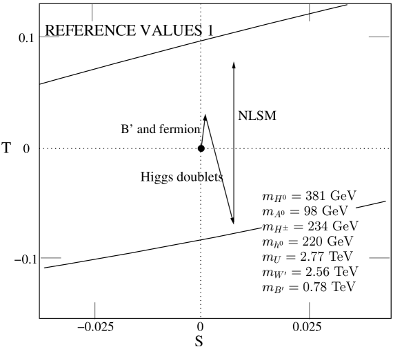
Figure 4: $S$ and $T$ values in the MMM for reference set 1 in Table 1 plotted on a 1.5-$\sigma$ oval in the S-T plane

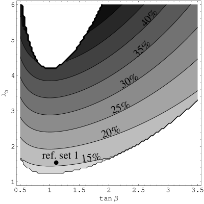
Figure 5: Fine tuning plotted as a function of $\tan(\beta)$ and $\lambda_{h}$ where all other parameters have been taken from Table 1. We only plot regions of parameter space which lie within the $S$-$T$ ellipse. We indicate the position of reference set 1. Note that the fine tuning improves for larger values of $\lambda_{h}$ as the Higgs becomes heavier.

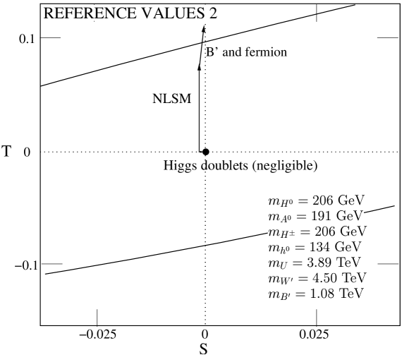
Figure 6: $S$ and $T$ values in the MMM for reference set 2 in Table 1 plotted on a 1.5-$\sigma$ oval in the S-T plane

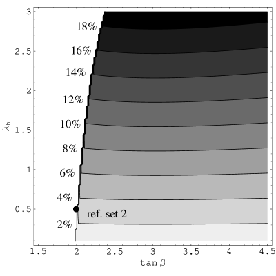
Figure 7: Fine tuning plotted as a function of $\tan{\beta}$ and $\lambda_{h}$ where all other parameters have been taken from Table 1. We plot regions of parameter space which are at least as close to the $S$-$T$ ellipse as reference set 2.

10 Conclusion

Little Higgs models, like the Minimal Moose, predict new heavy particles at the TeV scale. Upon integrating out these particles the SM is recovered at low energies, with possibly one or more extra Higgs doublets. At higher energies the Higgses form components of nonlinear sigma model fields which become strongly coupled at around 10 TeV. At still higher energies a UV completion of the theory is needed. This could be achieved with strongly coupled dynamics [14], a linear sigma model or supersymmetry. In the latter case the SUSY breaking scale is pushed to 10 TeV, alleviating the difficulties of flavor-changing neutral currents associated with TeV-scale superpartners.

At energies below the masses of these new particles we rely on precision electroweak data to gauge the feasibility of a particular model as a possible extension to the SM. In the absence of new flavor physics (due to the introduction of a partner for the top quark only), precision measurements can be divided into oblique and non-oblique corrections. We analyzed these for two such models at around a TeV, translating the low energy theory into effective operator language as far as possible. We saw that we ran into significant problems in more than one sector when we considered the constrained gauge structure of the MM. Gauging two copies of $SU(2)\times U(1)$ instead and charging the SM fermions equally under both U(1)s, as in the MMM, does away with these issues as we can then go to the near oblique limit without reintroducing large contributions to the $T$ parameter from $B^{\prime}$ exchange.

This might be understood better in the context of other LH theories, the Littlest Higgs [6] for example. The greatest contrast between this and the MM is the nonlinear sigma model sector, where the Littlest Higgs has a built-in $SU(2)_{c}$ symmetry which protects it from any $T$ parameter contribution. This symmetry is explicitly broken in the top sector, but only by a small amount. The gauge sectors of the theories are identical except for a $B^{\prime}$ mass in the Littlest Higgs which is lighter by a factor of 2 (since the theory only contains 1 link field), but heavier by $\sqrt{5/3}$ to account for the different group structure involved. Aside from this, the similarity in the general framework of the models implies that a lower cutoff can be tolerated in the case of the Littlest Higgs, giving rise to lower masses for the heavy particles, and a subsequent decrease in the level of fine tuning. The relative success of the MM is rather surprising, however, given that it was designed for minimality rather than freedom from precision electroweak constraints.

In summary we see that the MMM, which contains a gauged $\left[SU(2)\times U(1)\right]^{2}$ is a viable candidate for TeV-scale physics. The heavy counterparts for SM particles give rise to precision electroweak corrections that are within acceptable experimental bounds for a large range of parameters of the theory. It leads to at least moderate improvements over the SM in terms of the gauge hierarchy problem for generic regions of parameter space, and very significant improvements for less generic regions, which are nevertheless plausibly large. It remains for the LHC to confirm whether there is a role for Little Higgs theories in physics beyond the Standard Model.

Appendix A Top Seesaw

Starting with a top sector mass term of the form

$$-\left(\begin{array}[]{cc}\overline{t}&\overline{U}\end{array}\right)\left(\begin{array}[]{cc}m_{tt}&m_{tU}\\ m_{Ut}&m_{UU}\end{array}\right)\left(\begin{array}[]{c}\overline{t^{c}}\\ \overline{U^{c}}\end{array}\right)$$ (60)

we can diagonalize the $M^{{\dagger}}M$ matrix as in [15] giving mass eigenvalues of

$$m_{t,U}^{2}=\frac{1}{2}\left[m_{UU}^{2}+m_{tt}^{2}+m_{Ut}^{2}+m_{tU}^{2}\pm\sqrt{(m_{UU}^{2}+m_{tt}^{2}+m_{Ut}^{2}+m_{tU}^{2})^{2}-4(m_{UU}m_{tt}-m_{tU}m_{Ut})^{2}}\right]$$ (61)

with different mixing angles on the right and left

$$\left(\begin{array}[]{c}t^{\prime}\\ U^{\prime}\end{array}\right)=\left(\begin{array}[]{cc}c_{L}&-s_{L}\\ s_{L}&c_{L}\end{array}\right)\left(\begin{array}[]{c}t\\ U\end{array}\right)$$ (68)

$$\left(\begin{array}[]{c}\overline{t_{c}}^{\prime}\\ \overline{U_{c}}^{\prime}\end{array}\right)=\left(\begin{array}[]{cc}c_{R}&s_{R}\\ -s_{R}&c_{R}\end{array}\right)\left(\begin{array}[]{c}-\overline{t_{c}}\\ \overline{U_{c}}\end{array}\right)$$ (75)

and $c_{L}$ given by

$$\cos{\theta_{L}}=\frac{1}{\surd{2}}\left[1+\frac{m_{UU}^{2}-m_{tt}^{2}+m_{Ut}^{2}-m_{tU}^{2}}{m_{U}^{2}-m_{t}^{2}}\right]^{\frac{1}{2}}$$ (76)

References

- [1] Particle Data Group Collaboration, K. Hagiwara et. al., Review of particle physics, Phys. Rev. D66 (2002) 010001.
- [2] C. P. Burgess, S. Godfrey, H. Konig, D. London, and I. Maksymyk, Model Independent Global Constraints on New Physics, Phys. Rev. D49 (1994) 6115–6147, [hep-ph/9312291].
- [3] G. Altarelli, R. Barbieri, and F. Caravaglios, Electroweak Precision Tests: A Concise Review, Int. J. Mod. Phys. A13 (1998) 1031–1058, [hep-ph/9712368].
- [4] K. Hagiwara, S. Matsumoto, D. Haidt, and C. S. Kim, A Novel Approach to Confront Electroweak Data and Theory, Z. Phys. C64 (1994) 559–620, [hep-ph/9409380].
- [5] N. Arkani-Hamed et. al., The Minimal Moose for a Little Higgs, JHEP 08 (2002) 021, [hep-ph/0206020].
- [6] N. Arkani-Hamed, A. G. Cohen, E. Katz, and A. E. Nelson, The Littlest Higgs, JHEP 07 (2002) 034, [hep-ph/0206021].
- [7] T. Gregoire, D. R. Smith, and J. G. Wacker, What Precision Electroweak Physics Says About the SU(6)/Sp(6) Little Higgs, hep-ph/0305275.
- [8] S. Chang, A ‘Littlest Higgs’ Model with Custodial SU(2) Symmetry, hep-ph/0306034.
- [9] D. E. Kaplan and M. Schmaltz, The Little Higgs from a Simple Group, JHEP 10 (2003) 039, [hep-ph/0302049].
- [10] I. Low, W. Skiba, and D. Smith, Little Higgses from an Antisymmetric Condensate, Phys. Rev. D66 (2002) 072001, [hep-ph/0207243].
- [11] W. Skiba and J. Terning, A Simple Model of Two Little Higgses, Phys. Rev. D68 (2003) 075001, [hep-ph/0305302].
- [12] L. Lavoura and J. P. Silva, The Oblique Corrections from Vector - Like Singlet and Doublet Quarks, Phys. Rev. D47 (1993) 2046–2057.
- [13] J. F. Gunion, H. E. Haber, G. L. Kane, and S. Dawson, The Higgs Hunter’s Guide, . SCIPP-89/13.
- [14] A. E. Nelson, Dynamical Electroweak Superconductivity from a Composite Little Higgs, hep-ph/0304036.
- [15] R. S. Chivukula, B. A. Dobrescu, H. Georgi, and C. T. Hill, Top Quark Seesaw Theory of Electroweak Symmetry Breaking, Phys. Rev. D59 (1999) 075003, [hep-ph/9809470].
- [16] N. Arkani-Hamed, A. G. Cohen, and H. Georgi, Electroweak Symmetry Breaking from Dimensional Deconstruction, Phys. Lett. B513 (2001) 232–240, [hep-ph/0105239].
- [17] N. Arkani-Hamed, A. G. Cohen, T. Gregoire, and J. G. Wacker, Phenomenology of Electroweak Symmetry Breaking from Theory Space, JHEP 08 (2002) 020, [hep-ph/0202089].
- [18] S. Chang and J. G. Wacker, Little Higgs and Custodial SU(2), hep-ph/0303001.
- [19] J. G. Wacker, Little Higgs Models: New Approaches to the Hierarchy Problem, hep-ph/0208235.
- [20] T. Gregoire and J. G. Wacker, Mooses, Topology and Higgs, JHEP 08 (2002) 019, [hep-ph/0206023].
- [21] M. Perelstein, M. E. Peskin, and A. Pierce, Top Quarks and Electroweak Symmetry Breaking in Little Higgs Models, hep-ph/0310039.
- [22] M. E. Peskin and D. V. Schroeder, An Introduction to Quantum Field Theory, . Reading, USA: Addison-Wesley (1995) 842 p.
- [23] H.-J. He, C. T. Hill, and T. M. P. Tait, Top Quark Seesaw, Vacuum Structure and Electroweak Precision Constraints, Phys. Rev. D65 (2002) 055006, [hep-ph/0108041].
- [24] B. A. Dobrescu and C. T. Hill, Electroweak Symmetry Breaking via Top Condensation Seesaw, Phys. Rev. Lett. 81 (1998) 2634–2637, [hep-ph/9712319].
- [25] H. Collins, A. K. Grant, and H. Georgi, The Phenomenology of a Top Quark Seesaw Model, Phys. Rev. D61 (2000) 055002, [hep-ph/9908330].
- [26] R. Barbieri and A. Strumia, The ‘LEP Paradox’, hep-ph/0007265.
- [27] R. S. Chivukula, N. Evans, and E. H. Simmons, Flavor Physics and Fine-Tuning in Theory Space, Phys. Rev. D66 (2002) 035008, [hep-ph/0204193].
- [28] M. E. Peskin and T. Takeuchi, Estimation of Oblique Electroweak Corrections, Phys. Rev. D46 (1992) 381–409.
- [29] B. Grinstein and M. B. Wise, Operator Analysis for Precision Electroweak Physics, Phys. Lett. B265 (1991) 326–334.
- [30] C. Csaki, J. Hubisz, G. D. Kribs, P. Meade, and J. Terning, Variations of Little Higgs Models and their Electroweak Constraints, Phys. Rev. D68 (2003) 035009, [hep-ph/0303236].
- [31] C. Csaki, J. Hubisz, G. D. Kribs, P. Meade, and J. Terning, Big Corrections from a Little Higgs, Phys. Rev. D67 (2003) 115002, [hep-ph/0211124].
- [32] C. Csaki, Constraints on Little Higgs Models, . March 18th 2003 at Harvard University.
- [33] M. Schmaltz, Physics Beyond the Standard Model (Theory): Introducing the Little Higgs, Nucl. Phys. Proc. Suppl. 117 (2003) 40–49, [hep-ph/0210415].
- [34] S. Chang and H.-J. He, Unitarity of Little Higgs Models Signals New Physics of UV Completion, Phys. Lett. B586 (2004) 95–105, [hep-ph/0311177].