Information theory approach (extensive and nonextensive) to high energy multiparticle production processes

Abstract: We present an overview of information theory approach (both in its extensive and nonextensive versions) applied to high energy multiparticle production processes. It will be illustrated by analysis of single particle distributions measured in proton-proton, proton-antiproton and nuclear collisions. We shall demonstrate the particular role played by the nonextensivity parameter $q$ in such analysis as summarizing our knowledge on the fluctuations existed in hadronizing system.

PACS: 02.50.-r; 05.90.+m; 24.60.-k

Keywords: Information theory; Nonextensive statistics; Thermal models

1 Introduction

Information theory has been established to be extremely useful tool in many branches of science [1]. Its first application to multiparticle production processes is very old [2], however, it was used only sporadically since then [3, 4]. Here we shall present its methods and analyse, as example, single particle spectra obtained in multiparticle production processes at high energy [3, 4]. Such processes are responsible for the majority of observed cross section. If $k_{1,2}$ are four-momenta of colliding objects and $W=\sqrt{s}=\sqrt{\left(k_{1}+k_{2}\right)^{2}}$ is invariant energy of collision, then the mean multiplicity of produced secondaries increases with energy like $\langle N\rangle\propto\ln^{2}W$ or $\langle N\rangle\propto W^{\alpha}$ (with $\alpha\sim 0.5$) reaching in heavy ion collisions values of the order of $\sim 10^{3}\div\sim 10^{4}$. This fact makes analysis of such processes very difficult, in particular it is impossible to describe them from first principles. On the other hand, understanding these processes is very important because they provide background for more sophisticated measurements and they are themselves valuable source of information on the hadronization process in which initial energy $W$ converts into observed secondaries (mostly mesons $\pi$ and $K$). One is looking therefore for phenomenological models and first candidates were statistical models of different kinds [5, 6]. With necessary modifications and improvements they are actually in common use also nowadays and are very successful [7]. They all assume some kind of local thermal equilibrium forming at early stage of collision process. However, this assumption is not necessary because the characteristic ”thermal-like” (i.e., exponential) behaviour of some observables arises always whenether one restricts itself to observation of only a small part of some large system [8]. This is precisely situation encountered in multiparticle production processes where usually only a small part of produced secondaries is registered by detectors and out of them only very limited number is subjected to final analysis. The necessary averaging over all unmeasured degrees of freedom introduces therefore a kind of randomization or a heat bath, action of which can be summarily described by a single parameter $T$, a kind of ”effective temperature” of the usual thermodynamics [8]. It could, however, happen that such ”thermal bath” is more complicated (exhibiting, for example, some intrinsic fluctuations or collective flows) [9]. In such cases parameter $T$ must be supplemented by additional parameter summarily describing the action of these new factors - in this way the nonextensivity parameter $q$ appears (such ”heat baths” are not extensive anymore) [9] and notion of nonextensive statistics enters in a natural way [10].

Why use information theory methods in analysing multiparticle production processes? To illustrate this let us suppose that experiment measures some new distribution of secondaries. Immediately theoreticians rush to describe the new data and provide a number of models, which differ drastically in what concerns their assumptions, nevertheless they all do explain experimental results in a remarkable good way. What has happened? To answer this one has to introduce notion of information: data considered contain only limited amount of information and all models possess it as well. They differ therefore in what concerns additional redundant information they posses, which reflects not so much the state of the measured object but rather the state of minds of scientists proposing these models. To quantify this one has to resort to methods of information theory and introduce information entropy as a measure of information [1, 2, 3]. The problem one is facing can be formulated in following way. Suppose one has system S, depending on some variable $x\in(x_{min},x_{max})$, on which one performs finite number $n$ measurements providing us with $R_{1,\dots,n}$ results. The question is: how to obtain the most plausible (least biased) and model independent probability distribution, $p(x)$, of variable $x$? The answer is [1, 3]: look for such $p(x)$ (normalized to unity) which maximizes information entropy under constraints given by results of measurements. To account for many known features of the system under consideration (like long-range correlations, fractal-like structure of the phase space or intrinsic fluctuations, which will be of special interest to us later [11]) we shall use Tsallis entropy [10] characterised by parameter $q$, which for $q\rightarrow 1$ becomes the usual Shannon entropy [1]

$$S_{q}\,=\,-\frac{1}{1-q}\,\left[1\,-\,\int_{x_{min}}^{x_{max}}\,dx\,p(x)^{q}\right]\quad\stackrel{{\scriptstyle q\rightarrow 1}}{{\Longrightarrow}}\quad-\int_{x_{min}}^{x_{max}}\,dx\,p(x)\,\ln p(x),$$ (1)

under constraints

$$\int_{x_{min}}^{x_{max}}\,dx\,R^{(k)}(x)\cdot\left[p(x)\right]^{q}\,=\langle R^{(k)}\rangle_{q}=R^{(q)}_{k=1,\dots,n}.$$ (2)

As result one gets

$$p(x)\,=\,\frac{1}{Z_{q}}\exp_{q}\left[-\,\sum_{k=1}^{n}\beta^{(q)}_{k}\cdot R^{(k)}(x)\right],$$ (3)

where

$$\exp_{q}\left(\frac{x}{\Lambda}\right)\,=\,\left[1+(1-q)\frac{x}{\Lambda}\right]^{1/(1-q)}\qquad\stackrel{{\scriptstyle q\rightarrow 1}}{{\Longrightarrow}}\qquad\exp(\frac{x}{\Lambda}).$$ (4)

Here $\beta^{(q)}_{k}$ are Lagrange multipliers obtained by solving constraint equations and $Z_{q}$ ensures normalization of $p(x)$ to unity. It should be mentioned here that fluctuations in the parameter $1/\Lambda$ of the exponential distribution lead to the $q$-exponential with $q$ given by normalized variation of the parameter $1/\Lambda$ [11, 12].

Long time ago it was shown using this method (with $q=1$) [2] that in order to fit single particle distributions $dN/dy$ in rapidity variable $y=\frac{1}{2}\ln(E+p_{L})/\ln(E-p_{L})$ and multiparticle distributions $P(N;\bar{N})$ measured at that time it was enough to assume that: $(i)$ transverse momenta of produced secondaries $p_{T}$ are limited (i.e., phase space is effectively one dimensional) and $(ii)$ not the whole available energy $\sqrt{s}$ is used for production of the observed secondaries but only its fraction $K\in(0,1)$ called inelasticity, the rest of energy is taken away by the so called ”leading particles”. Closer scrutiny of numerous models competing at that time revealed that all of them contained these two assumptions (explicitly or implicitly) and that these assumptions consisted the only part common to all of them. All other additional assumptions were spurious and unnecessary and as such could be safely abandoned without spoiling agreement with data.

2 Results

We shall present now examples of analysis of single particle distributions in rapidity for $pp$ and $p\bar{p}$ collisions at energies varying between $\sqrt{s}=20$ GeV to $1800$ GeV [4] and first results for central nuclear collisions (see Fig. 1). Our input consists of: $(i)$ the energy of collision, $E_{cm}=\sqrt{s}$, out of which, according to result of [2], we shall retain only fraction $K_{q}$ for production of secondaries; $(ii)$ the mean multiplicity of charged secondaries produced in nonsingle diffractive reactions at given energy: $\bar{n}_{ch}=-7.0+7.2s^{0.127}$ (out of which we construct the total number of produced particles, $N=\frac{3}{2}\bar{n}_{ch}$ needed in our procedure); $(ii)$ the fact that phase space is essentially one dimensional with mean transverse momentum slightly energy dependent given by $\langle p_{T}\rangle=0.3+0.044\ln\left(\sqrt{s}/20\right)$ [13] (all secondaries will be assumed to be pions of mass $\mu=0.14$ GeV) and $(iv)$ that multiplicity distributions of produced secondaries is not Poissonian (like it was in [2]) but of Negative Binomial (NB) type

$$P(n)\,=\,P(n;\bar{n},k)\,=\,\frac{\Gamma(k+n)}{\Gamma(1+n)\Gamma(k)}\cdot\frac{\gamma^{k}}{(\gamma+1)^{k+n}}\qquad{\rm with}\qquad\gamma=\frac{k}{\bar{n}},$$ (5)

where parameter $k$ ($k\geq 1$) affects width of $P(n)$ and is given by its normalized variance [13]

$$\frac{1}{k}\,=\,\frac{\sigma^{2}\left(n_{ch}\right)}{\langle n_{ch}\rangle^{2}}-\frac{1}{\langle n_{ch}\rangle}\,=\,-0.104+0.058\ln\sqrt{s}.$$ (6)

This last point is new and most important because it can be accounted for only in nonextensive version of our method with $q>1$. This is because the value of $k^{-1}$ may be understood as the measure of fluctuations of mean multiplicity caused by some dynamical factors. When there are only statistical fluctuations in hadronizing system then $P(n)$ is of Poissonian type. Intrinsic (dynamical) fluctuations would mean fluctuating mean multiplicity $\bar{n}$. In the case when such fluctuations are given by a gamma distribution with normalized variance $D(\bar{n})$ then, as a result, one obtains the NB multiplicity distribution with $1/k=D(\bar{n})$ (because convolution of Poissonian and Gamma distributions results in NB one [17]). Assuming now that these fluctuations contribute to nonextensivity, i.e., that they define parameter $q=1+D(\bar{n})$, one is lead to the use of $q>1$ (i.e., nonextensive formalism) with $q=1+1/k$, where $k$ is parameter defining NB form of $P(n)$, energy dependence of which is given by. eq. (6).

With such input the most probable rapidity distribution is

$$p(y)\,=\,\frac{1}{N}\frac{dN}{dy}\,=\,\frac{1}{Z_{q}}\exp_{q}\left(-\beta_{q}\cdot\mu_{T}\cosh y\right),$$ (7)

where $Z_{q}$ and $\beta_{q}$ are not free parameters, like in similar formulas used in applications of statistical models [18], but are given by the normalization condition and by the energy conservation constraint ($\mu_{T}=\sqrt{\mu^{2}+\langle p_{T}\rangle^{2}}$, see [4] for details):

$$\int_{-Y_{m}}^{Y_{m}}\,dy\,\mu_{T}\cdot\cosh y\cdot[p(y)]^{q}\,=\,\frac{\kappa_{q}\cdot\sqrt{s}}{N}.$$ (8)

Symmetry of the collision (identical particles) implies that momentum is conserved in this case automatically. There are therefore two parameters, nonextensivity $q$ responsible for fluctuations (as mentioned above) and $q$-inelasticity $\kappa_{q}$ to be deduced directly from data essentially in a model independent way, cf. Fig. 1a. There is, however, question concerning physical meaning of $\kappa_{q}$ for $q>1$ case considered here (notice that our $q$ changes from $1.05$ to $1.33$ when going from $\sqrt{s}=20$ GeV to $1800$ GeV whereas the ”partition temperature” $T_{q}=1/\beta_{q}$ changes, accordingly, from $1.76$ GeV to $62.57$ GeV [4]). The point is, as was stressed in [19], that in case of $q>1$ our energy $\kappa_{q}$ contains also interaction between particles and is not directly seen in rapidity distribution. However, the quantity (inelasticity)

$$K_{q}=\frac{N}{\sqrt{s}}\langle E_{q}\rangle\,=\,\frac{N}{\sqrt{s}}\cdot\int_{-Y_{m}}^{Y_{m}}dy\,p(y)\left[\mu_{T}\cdot\cosh y\right]\,\sim\,\frac{\kappa_{q}}{3-2q}$$ (9)

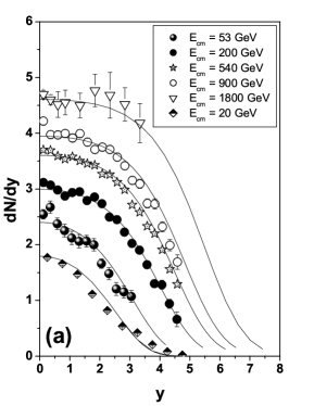
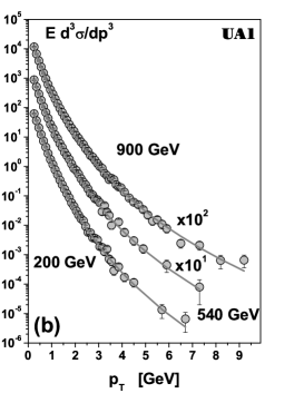
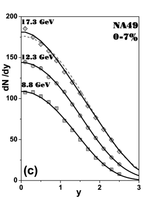
Figure 1: Examples of applying eq. (3). $(a)$ fit to rapidity spectra for charged pions produced in $pp$ and $\bar{p}p$ collisions at different energies [14]. $(b)$ fit to $p_{T}$ spectra from UA1 experiment [15]. $(c)$ fits to rapidity spectra for negatively charged pions produced in $PbPb$ collisions at different energies (for the most central $0-7\%$ interval of impact parameter of collision [16]). The best fit for $17.3$ GeV is for two-source case, cf. Fig. 2f, with $q=1$ and $\Delta y=0.83$. Total inelasticity in this case is $K=0.58$. See text for other details.

is the correct fraction of energy used for production of secondaries particles (it happens to be fairly constant with $\sqrt{s}$ varying slightly around $K_{q}\sim 0.5$ [4]). Fig. 1b shows example of similar fit but this time to the observed $p_{T}$ spectra at energies $200$, $500$ and $900$ GeV [15] (using eq. (7) with energy $\mu_{T}\cosh y$ replaced by transverse momentum $p_{T}$). As can be noticed fits are very good in the whole range of $p_{T}$ with the corresponding values of $T_{T}=1/\beta_{T}$ (in GeV) and $q_{T}$ equal to $(T_{T};q_{T})=(0.134;1.095)$, $(0.135;1.105)$ and $(0.14;1.11)$ for energies $200$, $500$ and $900$, respectively. These values must be compared with the corresponding values of $(T=T_{L};q=q_{L})$ for rapidity distributions, which are equal to, respectively: $(11.74;1.2)$, $(20.39;1.26)$ and $(30.79;1.29)$ at comparable energies [4]. The question then arises, what is the actual value of the parameter $q$ describing fluctuations of the mean multiplicity, i.e., affecting, according to the previous discussion, multiplicity distributions? It is sensitive to $p=\sqrt{p^{2}_{L}+p^{2}_{T}}$ and, as we have seen here, both $p_{L}$ and $p_{T}$ show traces of fluctuations by leading to $q>1$. At present we can offer only some approximate answer because there are no data measuring $p_{T}$ distributions at all values of rapidity $y$, i.e., providing correlations between parameters $(T;q)=(T_{L};q_{L})$ for longitudinal momenta (rapidity) distributions and $(T;q)=(T_{T};q_{T})$ for transverse momenta distributions. Noticing that $q-1=\sigma^{2}(T)/T^{2}$ (i.e., it is given by fluctuations of total temperature $T$) and assuming that $\sigma^{2}(T)=\sigma^{2}(T_{L})+\sigma^{2}(T_{T})$, one can estimate that resulting values of $q$ should not be too different from

$$q\,=\,\frac{q_{L}\,T_{L}^{2}\,+\,q_{T}\,T^{2}_{T}}{T^{2}}\,-\,\frac{T^{2}_{L}\,+\,T^{2}_{T}}{T^{2}}\,+\,1,$$ (10)

which, for $T_{L}\gg T_{T}$, as is in our case, leads to the result that $q\sim q_{L}$, i.e., it is given by the longitudinal (rapidity) distributions only.

Finally, on Fig. 1c we show fits to the recent NA49 data [16] on $\pi^{-}$ production in $PbPb$ collisions at three different energies (per nucleon). The values of $(q;K_{q}=3\cdot K^{(\pi^{-})}_{q})$ obtained are: $(1.2;0.33)$ for $17.3$ GeV, $(1.164;0.3)$ for $12.3$ GeV and $(1.04;0.22)$ for $8.6$ GeV. The origin of $q>1$ in this case is not yet clear. The inelasticity seems to grow with energy. It is also obvious that for higher energies some new mechanism starts to operate because we cannot obtain in this case agreement with data using only the energy conservation constraint. The possibility offered in this matter by some closer inspection of properties of eqs. (3) and (7) are displayed in Fig. 2. Whereas upper panels are self-explanatory, the lower demand some attention. They show how $p(y)$ can be distorted and it could be that one of the mechanisms presented there is showing up in high energy NA49 data mentioned above. Three mechanisms are listed there (only $q=1$ case is considered). Fig. 2d shows the changes in $p(y)$ introduced by $y$-dependent $p_{T}$, especially when $\langle p_{T}\rangle$ grows substantially towards $y=0$ (in such a way as to keep the averaged $\langle p_{T}\rangle$ the same as original $0.4$ GeV/c). In this case one observes increase of $p(y)$ at small values of $y$ but it seems to be too wide to explain the NA49 data.

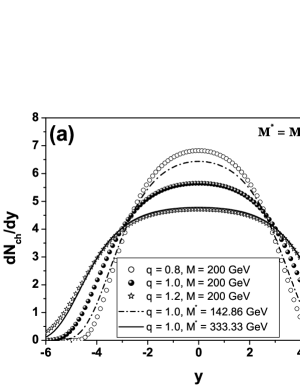
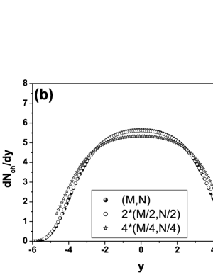
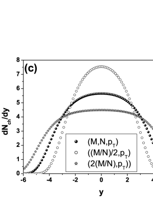
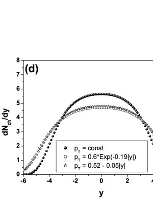
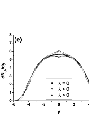
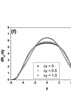
Figure 2: Examples of properties of eqs. (3) ($W=200$ GeV, $N=60$, $\langle p_{T}\rangle=0.4$ GeV/c). $(a)$ spectra obtained for different parameter $q$ practically coincide with extensive spectra produced by masses $M^{\star}=M/(3-2q)$. For all remaining panels $q=1$. $(b)$ quasiscaling for spectra obtained for composition of smaller masses producing respectively smaller number of secondaries with $M/N=$const. $(c)$ spectra with different values of $M/N$ ratio differ drastically. $(d)$ the $p_{T}$ growing towards the center of rapidity phase space has dramatic effect on spectra. $(e)$ the role of momentum dependent residual interaction (cf. eq. (11)) is visualised. $(f)$ the effect of two sources separated in rapidity by $2\Delta y$ with combined energies and masses equal $M$ is visualised.

Fig. 2e shows result of the special kind of momentum dependent residual interactions discussed in [20]. In our case it would result in

$$p(y)=\frac{1}{Z}\cdot\exp\left[-\beta\cdot\mu_{T}\cosh y\,-\,\lambda\cdot\mu_{T}|\sinh y|\right]$$ (11)

with additional constraint imposed now on the modulus of the momenta:

$$\int_{-Y_{m}}^{Y_{m}}\,dy\,\mu_{T}|\sinh y|\,p(y)\,=\kappa\cdot\frac{\sqrt{W^{2}-M^{2}}}{N}.$$ (12)

Here $W=K\cdot\sqrt{s}$ and $M=\sum_{i}\sqrt{\mu_{T}^{2}+p_{Li}^{2}}$ with $p_{Li}=\mu_{T}\sinh y_{i}$ (sum is over all produced particles, $i=1,\dots,N$, and $\kappa$ is parameter telling us the fraction of momentum turned into interaction). As it can be seen in Fig. 2e, the effect of this interaction although visible is very weak and probably negligible at present data.

The most promising seems to be the conjecture that invariant energy $W=K\cdot\sqrt{s}$ hadronizing into $N$ particles consists in reality with two subsources of energies $W_{1}=W_{2}$, which are displaced from $y=0$ by some rapidity $\Delta y$ (being a free parameter here) and producing $N/2$ particles each, $W_{1,2}=W/[2\cosh(\Delta y)]$. As one can see, the obtained shape is very similar to what is observed experimentally (cf. Fig. 1c).

3 Summary

In some types of data on multiparticle production processes one frequently encounters ambiguity concerning the question, which of the particular models used at that time is the correct one [2]. Such situation arises always when data contain only limited amount of information. To select this information one has apply information theory methods, which are widely known and used in other branches of science [1]. The examples shown here show that information theory ideas can be successfully used also to analyse data from multiparticle production processes and that in this way one gets highly model independent estimation of some quantities, in our example it was inelasticity parameter $K$ [4]. Actually, in [21] we have attempted to fit single particle distribution without a priori introducing neither inelasticity nor fluctuations in mean multiplicity and found that it is possible only with $q<1$. The reason turned out to be simple: in this case the most important factor was decreasing of the available phase space to mimic the action of the inelasticity and this can be done only with $q<1$. The fit was not as good as shown here with notion of inelasticity introduced explicitly but it was not very bad either. As in [11, 12] we are stressing here the connection between necessity to use nonextensive version of information theory and some intrinsic fluctuations existing in the hadronizing system. Finally, as was clearly displayed in Fig.2, our method seems to be also very useful in describing the gross features of the single particle spectra observed in heavy ion collisions. In particular, it seems that with growing energy of collision there is room for some new mechanisms, not present at more elementary nucleonic collisions. This point deserves therefore some special scrutiny in the future.

We would like to finish mentioning that there exists also example of very successful use of the information theory approach to describe not only single but also double particle spectra, namely the so called Bose-Einstein correlations observed between identical bosons in all multiparticle production data, see [22].

Acknowledgments: GW is grateful to the organizers of the NEXT2003 for their support and hospitality. Partial support of the Polish State Committee for Scientific Research (KBN) (grant 2P03B04123 (ZW) and grants 621/E-78/SPUB/CERN/P-03/DZ4/99 and 3P03B05724 (GW)) is acknowledged.

References

- [1] P.Harremoës and F.Topsøe, Entropy 3 (2001) 191 and references therein.
- [2] Y.-A.Chao, Nucl. Phys. B40 (1972) 475.
- [3] G.Wilk and Z.Włodarczyk, Phys. Rev. D50 (1994) 2318.
- [4] F.S.Navarra, O.V.Utyuzh, G.Wilk and Z.Włodarczyk, Phys. Rev. D67 (2003) 114002.
- [5] W.Heisenberg, Z. Phys. 126 (1949); E.Fermi, Prog. Theor. Phys. 5 (1950); I.Pomeranczuk, Dokl. Akad. Nauk SSSR 78 (1951) 889; L.D.Landau and S.Z.Bilenkij, Nuovo Cim. Suppl. 3 (1956) 15.
- [6] R.Hagedorn, Nuovo Cim. Suppl. 3 (1965) 147; Nuovo Cim. A52 (1967) 64 and Riv. Nuovo Cim. 6 (1983) 1983.
- [7] Cf., for example: U.Heinz, J. Phys. G25 (1999) 263; F.Becattini, Nucl. Phys. A702 (2002) 336 and F.Becattini and G.Passaleva, Eur. Phys. J. C23 (2002) 551; W.Broniowski, A.Baran and W.Florkowski, Acta Phys. Polon. B33 (2002) 4235; T.Csörgő, F.Grassi, Y.Hama and T.Kodama, Phys. Lett. B565 (2003) 107 (and further references therein).
- [8] L.Van Hove, Z. Phys. C21 (1985) 93 and C27 (1985) 135.
- [9] A.R.Plastino and A.Plastino, Phys. Lett. A193 (1994) 140; M.Baranger, Physica A305 (2002) 27; A.K.Aringazin and M.I.Mazhitov, Physica A325 (2003) 409; M.P.Almeida, Physica A325 (2003) 426.
- [10] C.Tsallis, in Nonextensive Statistical Mechanics and its Applications, S.Abe and Y.Okamoto (Eds.), Lecture Notes in Physics LPN560, Springer (2000). See also at http://tsallis.cat.cbpf.br/biblio.htm.
- [11] G.Wilk and Z.Włodarczyk, Phys. Rev. Lett. 84 (2000) 2770; Chaos, Solitons and Fractals 13/3 (2001) 581.
- [12] C.Beck and E.G.D.Cohen, Physica A322 (2003) 267
- [13] C.Geich-Gimbel, Int. J. Mod. Phys A4 (1989) 1527.
- [14] C.De Marzo et al., Phys. Rev. D26 (1982) 1019 and D29 (1984) 2476; R.Baltrusaitis et al., Phys. Rev. Lett. 52(1993) 1380; F.Abe et al., Phys. Rev. D41 (1990) 2330.
- [15] C.Albajar et al. (UA1 Collab.) Nucl. Phys. B335 (1990) 261.
- [16] S.V.Afanasjev et al. (NA49 Collab.), Phys. Rev. C66 (2002) 054902.
- [17] P.Carruthers and C.S.Shih, Int. J. Mod. Phys. A2 (1986) 1447.
- [18] T.T.Chou and C.N.Yang, Phys. Rev. Lett. 54 (1985) 510 and Phys. Rev. D32 (1985) 1692.
- [19] C.Beck, Physica A286 (2000) 164.
- [20] B.Schenke and C.Greiner, Statistical description with anisotropic distributions for hadron production in nucleus-nucleus collisions, nucl-th/0305008. See also: L.W.Neise, H.Stöcker and W.Greiner, J. Phys. G13 (1987) L181.
- [21] F.S.Navarra, O.V.Utyuzh, G.Wilk and Z.Włodarczyk, Nuovo Cim. 24C (2001) 725.
- [22] T.Osada, M.Maruyama and F.Takagi, Phys. Rev. D59 (1999) 014024.