BEYOND BFKL

Abstract

The Balitsky-Fadin-Kuraev-Lipatov (BFKL) evolution equation is known to be “unstable” with respect to fluctuations in gluon virtuality, transverse momentum and energy requiring to go beyond the leading order BFKL. Still, these instabilities point to fruitful improvements of our deep understanding of QCD. Recent applications to next-leading order and to saturation problems are outlined.

1 “Instabilities” of the BFKL Equation

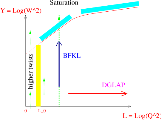
Figure 1: The QCD evolution landscape. The BFKL evolution and its limitations. i) to the left: non-perturbative region; ii) to the right: DGLAP evolution; iii) to the top: Saturation region.

The Balitsky-Fadin-Kuraev-Lipatov (BFKL) evolution equation has already a venerable past[1]. It appears as a key tool in many recent works on small-x physics (in the broad sense). It is interesting to notice that its limitations themselves are the seeds of interesting fields of research. Let us discuss limitations which can be associated with the idea of “instabilities”.

• i) Instability towards the non-perturbative regime

  It is well known that the perturbative “gluon ladder” contributing to the BFKL cross-section is characterized by a “cigar-shape” structure[2] of the transverse momenta. Hence, it is difficult to avoid an excursion inside the near-by non-perturbative region

  (Fig. (1), to the left).

• ii) Instability towards the renormalization group regime

  Calculations of the next-leading BFKL kernel[3] has proven that the inclusion of next-leading logs gives a (too) strong correction to the leading log result. After a resummation motivated by the suppression of spurious singularities[4, 5], the results show that the resummed NLO-BFKL kernels are very similar, e.g. “attracted” towards the Dokshitzer Gribov Lipatov Altarelli Parisi (DGLAP) evolution[6] , at least for the structure functions

  (Fig. (1), to the right).

• iii) Instability towards the high density (saturation) regime

  The BFKL evolution implies a densification of gluons and sea quarks, while they keep in average the same size. It is thus natural to expect[7] a modification of the evolution equation by non-linear contributions in the gluon density. Recently, the corresponding theoretical framework has been settled[8, 9], and is based on an extension of the BFKL kernel acting on non-linear terms. It leads to a transition to the saturation regime (Fig. (1), to the top).

The main subjects of my talk will concern contributions to point (ii), with a discussion of the phenomenological relevance of (resummed) NLO-BFKL kernels and point (iii), with a discussion of traveling wave solutions of non-linear QCD equations, as being deeply related to geometric scaling and the transition to saturation.

2 “Instability towards DGLAP”

The “instability” of the BFKL equation’s solution w.r.t. the renormalization group evolution is well-known[12]. Indeed, the first correction to the leading-$\log 1/x$ approximation of the BFKL kernel[3] is large enough to apparently endanger the whole BFKL approach. It was soon realized that a large part of the problem was due to the appearance of singularities which contradict the renormalization group properties. Hence requiring an harmonization between the next leading log BFKL calculations and the renormalization group requirements through higher orders’ resummation leads[4, 5] to a possible way out of the problem.

Let us focus[13] on the impact of these developments on the proton structure functions

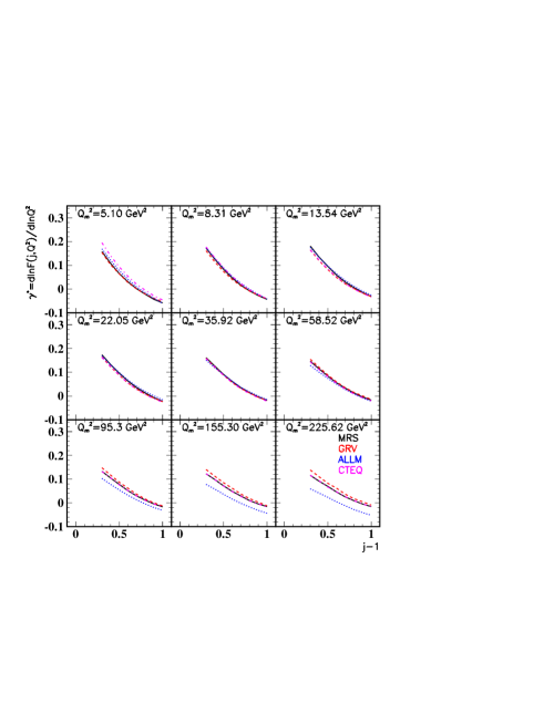
Figure 2: $\bar{\gamma}(\omega,Q^{2}):$ The “effective” $F_{2}$ anomalous dimension. $\bar{\gamma}(\omega,Q^{2})$ has been evaluated from four known different parametrizations. They are all compatible in the range $.3<\omega<1,5<Q^{2}<100\ GeV^{2},$ where we restrict our analysis.

and recall the parametrization of the proton structure functions in the (LO) BFKL approximation[14]:

$$F_{i}=\int\frac{d\gamma}{2i\pi}\left(\frac{Q^{2}}{Q_{0}^{2}}\right)^{\gamma}{x_{Bj}}^{-\frac{\alpha_{s}N_{c}}{\pi}\chi_{L0}(\gamma)}\ h_{i}(\gamma)\ \eta(\gamma)\ ,$$ (1)

where $F_{i}$ denotes respectively $F_{T},\ F_{L},\ G$ (resp. transverse, longitudinal and gluon) structure functions and $h_{i}$ are the known perturbative couplings to the photon ($h_{G}\!=\!1$ for the gluon structure function), usually called “impact factors”[15].

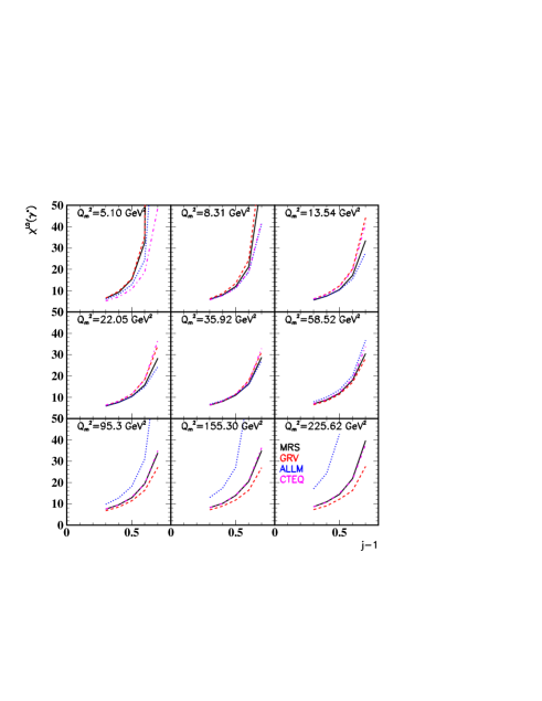
Figure 3: Test of Relation ii): LO-BFKL.

$\chi_{L0}$ is the the LO-BFKL kernel, $\alpha_{s}$ the (fixed) coupling constant and $\omega(\gamma)$ an (unknown but factorizable[15]) non-perturbative coupling to the proton.

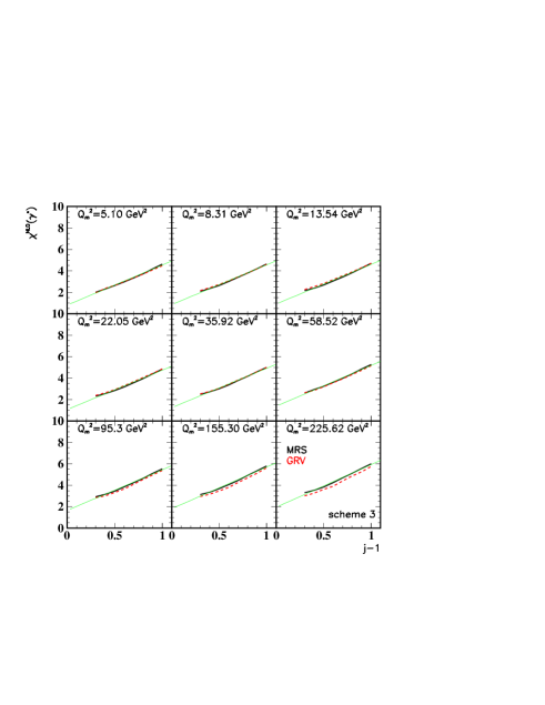
Figure 4: Test of Relation ii): NLO-BFKL.

Mellin-transforming (1) in $j\!-\!1\equiv\omega$ space, one easily finds

$$\tilde{F}_{i}=\int\frac{d\gamma}{2i\pi}\left(\frac{Q^{2}}{Q_{0}^{2}}\right)^{\gamma}\frac{1}{\omega-\frac{\alpha_{s}N_{c}}{\pi}\chi_{L0}(\gamma)}\ h_{i}(\gamma)\ \eta(\gamma)\ ,$$ (2)

and, taking the pole contribution, one has the important relation

$$\omega=\frac{\alpha_{s}N_{c}}{\pi}\chi_{L0}(\gamma_{k}(\omega))\ .$$ (3)

Let us try and find the equivalent relation at NLO. At (resummed) next-to-leading order, one can similarly write

$$\tilde{F}_{i}=\int\frac{d\gamma}{2i\pi}\left(\frac{Q^{2}}{\Lambda_{QCD}^{2}}\right)^{\gamma}e^{-\frac{\ X(\gamma,\omega)}{b\omega}}\ h_{i}(\gamma,\omega)\ \eta(\gamma,\omega)\ ,$$ (4)

where, by construction

$${\partial\over\partial\gamma}X(\gamma,\omega)\equiv\chi_{NLO}(\gamma,\omega)\ .$$ (5)

The function $X(\gamma,\omega)$ appears in the solution of the Green function derived from the renormalization-group improved small-$x_{Bj}$ equation[4], $\chi_{NLO}(\gamma,\omega)$ is a resummed NLO-BFKL kernel and

$$\frac{N_{c}}{\pi}\ \alpha_{s}(Q^{2})=\left[{b\ln\left(Q^{2}/\Lambda_{QCD}^{2}\right)}\right]^{-1}\ ,$$ (6)

with $b=11\!-\!2/3\ N_{f}/N_{c}.$

At large enough $Q^{2}/\Lambda_{QCD}^{2},$ one can use the saddle-point appoximation in $\gamma$ to evaluate (4). Assuming that the perturbative impact factors and the non-perturbative function $\eta$ do not vary much, the saddle-point condition reads

$$\omega\sim\frac{\chi_{NLO}(\bar{\gamma},\omega)}{b\ \ln\left(Q^{2}/\Lambda_{QCD}^{2}\right)}\ =\frac{N_{c}\ \alpha_{s}(Q^{2})}{\pi}\chi_{NLO}(\bar{\gamma},\omega)\ ,$$ (7)

where $\bar{\gamma}\equiv\bar{\gamma}(\omega,Q^{2})$ is the saddle-point value.

Inserting the saddle point defined by (7) in formula (4), one obtains a set of conditions to be fulfilled at (resummed) NLO level as follows:

i) The Mellin transform $\tilde{F}_{2}\equiv\tilde{F}_{T}+\tilde{F}_{L}$ defines:

$${\partial\over\partial\ln({Q^{2}})}\ln\tilde{F}_{2}(\omega,{Q^{2}})\ \sim\ \bar{\gamma}(\omega,Q^{2})\ .$$ (8)

ii) $\bar{\gamma}$ verifies

$$\chi_{NLO}(\bar{\gamma})\equiv\frac{\pi\ \omega}{\alpha_{s}(Q^{2})N_{c}}\ ,$$ (9)

where $\chi_{NL0}$ is a resummed NLO-BFKL kernel.

iii) The gluon structure function (one may also choose the obervable $F_{L}$) verifies, via Mellin transform:

$$\ln(\tilde{G}(\omega,Q^{2}))=\ln\left(\tilde{F_{2}}(\omega,Q^{2})\right)-\bar{\gamma}\ \ln\left[h_{T}(\bar{\gamma})+h_{L}(\bar{\gamma})\right]\ .$$ (10)

We test[13] the properties i)-iii) using NLO kernels proposed in[4], and compared with the LO kernel condition (3).

As an example an extraction of an “effective” $F_{2}$ anomalous dimension i), see Fig. (2), is performed[13] using different parametrisations in a range of $\omega$ verifying the stability with respect to cuts on unknown (smallest) or irrelevant (large) $x_{Bj}.$ The comparison of the property ii) to the LO BFKL kernel is displayed in Fig.(3) and the one with a resummed NLO-BFKL kernels (cf. Scheme[4] 3) in Fig.(4). As is clearly seen on the figures the Mellin-transform analysis disfavors the BFKL-LO kernel, while it is qualitatively compatible with the resummed BFKL-NLO kernel. The remaining discrepancies at NLO could be attributed to finite NNLO corrections to the kernel or to still unknown NLO contributions to the impact factors[16]. A systematic study of the proposed NLO kernels is thus made possible using the method.

3 “Saturation instability”

As well-known, the BFKL evolution (even including next-leading contributions) leads to a multiplication of partons with non-vanishing size and thus inevitably leads to a dense medium . This may be called the “Saturation Instability” of the BFKL evolution.

The back-reaction of parton saturation on the BFKL equation has been originally[7] described by adding a non-linear damping term. More recently, the evolution equation to saturation have been theoretically derived in the case of scattering on a “large nucleus”, e.g. when the development of the parton cascade is tested by uncorrelated probes[8, 9].

In the following we will focus on the solutions of the Balitsky-Kovchegov (BK) equations[9] where one consider the evolution within the QCD dipole Hilbert space[17]. To be specific let us consider $N(Y,{x}_{01}),$ the dipole forward scattering amplitude and define

$${\mathbb{N}}(Y,k)=\int_{0}^{\infty}\frac{dx_{01}}{x_{01}}J_{0}(kx_{01})\,N(Y,x_{01})\ .$$ (11)

Figure 5: Typical traveling wave solution. The function $u(t,x)$ is represented for three different times. The wave front connecting the regions $u=1$ and $u=0$ travels from the left to the right as $t$ increases. That illustrates how the “strong absorption” or saturated phase region invades the “transparency” region.

Within suitable approximations (large $N_{c}$, summation of fan diagrams, spatial homogeneity) and starting from the Balitsky-Kovchegov equation[9], it has been shown that this quantity obeys the nonlinear evolution equation

$${\partial_{Y}}{\mathbb{N}}=\bar{\alpha}\chi\left(-\partial_{L}\right){\mathbb{N}}-\bar{\alpha}\,{\mathbb{N}}^{2}\ ,$$ (12)

where $\bar{\alpha}=\alpha_{s}N_{c}/\pi$, $\chi(\gamma)=2\psi(1)-\psi(\gamma)-\psi(1\!-\!\gamma)$ is the characteristic function of the BFKL kernel[1], $L=\log(k^{2}/k_{0}^{2})$ and $k_{0}$ is some fixed low momentum scale. It is well-known that the BFKL kernel can be expanded to second order around $\gamma\!=\!{\scriptstyle\frac{1}{2}}$, if one sticks to the kinematical regime $8\bar{\alpha}Y\gg L$. We expect this commonly used approximation to remain valid for the full nonlinear equation. The latter boils down to a parabolic nonlinear partial derivative equation:

$${\partial_{Y}}{\mathbb{N}}=\bar{\alpha}\bar{\chi}\left(-\partial_{L}\right){\mathbb{N}}-\bar{\alpha}\,{\mathbb{N}}^{2}\ ,$$ (13)

with

$$\bar{\chi}\left(-\partial_{L}\right)=\chi\left({\scriptstyle\frac{1}{2}}\right)+\frac{\chi^{\prime\prime}\!\left({\scriptstyle\frac{1}{2}}\right)}{2}\left(\partial_{L}+{\scriptstyle\frac{1}{2}}\right)^{2}\ .$$ (14)

The key point of our recent approach[18] is to remark that the structure of Eq.(13) is identical (for fixed $\alpha$) to a mathematical and physical archetype of non-linear evolution equation for which useful tools can be applied, namely the Fisher and Kolmogorov-Petrovsky-Piscounov (KPP) equation[19] for a function $u$:

$$\partial_{t}u(t,x)=\partial_{x}^{2}u(t,x)+u(t,x)(1-u(t,x))\ ,$$ (15)

which is directly related[18] to ${\mathbb{N}}.$ The equation can be generalized to many physical situations, including running $\alpha.$

Figure 6: Evolution of the reduced front profile. Fixed coupling: left; Running coupling: right. The reduced front profile $(k^{2}/Q_{s}^{2})^{\gamma_{c}}\,{\mathbb{N}}(k/Q_{s}(Y),Y)$ is plotted against $\log(k^{2}/Q_{s}^{2})$ for different rapidities. The various lines correspond to rapidities from 2 (lower curves, full line) up to 10 (upper curves). Note the similarity of the wave fronts, but the quicker time evolution (in $\sqrt{t}$) for fixed coupling, by contrast with the slow time evolution (in $t^{1/3}$) for the running coupling case.

Our main results are the following. The well-known geometric scaling property[20] is obtained for the solution of the non-linear equation (13) for the gluon amplitude at large energy. In our notation, the geometric scaling property reads

$${\mathbb{N}}(Y,k)={\mathbb{N}}\left(\frac{k^{2}}{Q_{s}^{2}(Y)}\right)\ ,$$ (16)

where $Q_{s}^{2}(Y)$ is the saturation scale. We prove that geometric scaling is directly related to the existence of traveling wave solutions of the KPP equation[19] at large times. This means that there exists a function of one variable $w$ such that

$$u(t,x)\underset{t\rightarrow+\infty}{\sim}w(x-m{(t)})$$ (17)

uniformly in $x$. Such a solution is depicted on Fig.(5). The function $m{(t)}$ depends on the initial condition. For the QCD case[18], one has to consider

$$m{(t)}=2t-{\scriptstyle\frac{3}{2}}\log t+{\mathbb{O}}(1)\ .$$ (18)

When transcribed in the appropriate physical variables, this mathematical result, implies directly the known geometric scaling properties[18]. It is interesting to note how the traveling wave solutions provide a particularly striking mathematical realization of an “instability” as depicted in Fig.(5), when a stable fixed point (strong absorption) “invades” an unstable one (transparency).

This mathematical analysis can be extended[18] to the study of the transition towards geometrical scaling , i.e. the formation of the front wave as a function of time, both for fixed and running $\alpha,$ see Fig.(6).

4 Conclusion

In the present contribution, we have discussed some aspects of the “instabilities” of the BFKL equations, i.e.:

• i) Instability towards the non-perturbative regime

• ii) Instability towards the renormalization group regime

• iii) Instability towards the high density (saturation) regime

At first sight, these instabilities could have appeared as drawbacks of the whole approach. On the very contrary, we have seen that the extensions of BFKL equation raised up by the treatment of “instabilities” appear to be the building blocks of most interesting recent developments towards a better understanding of QCD dynamics. As an example, I chose to present some personal recent contributions to this discussion, which are far from giving an idea of the whole extent of the works which attack the problem nowadays.

As a brief outlook, let us mention:

About Point (i), not discussed here, let us mention the formal but informative discussion on the $N=4$ supersymmetric QCD field theory and the AdS/CFT correspondence[11].

Point (ii): It is the subject of a developing activity which will allow to master the rather high technicality of the BFKL-NLO calculations and thus to penetrate the subtle aspects of the compatibility between BFKL and DGLAP evolution equations.

Point (iii): Saturation with both its phenomenological and theoretical aspects will certainly retain the attention of the Particle Physics community. The challenge here is the quest for a new phase of intense QCD fields and the undersatanding of its dynamical properties.

References

- [1] L.N.Lipatov, Sov.J.Nucl.Phys. 23 (1976) 642; V.S.Fadin, E.A.Kuraev and L.N.Lipatov, Phys. Lett. B60 (1975) 50; E.A.Kuraev, L.N.Lipatov and V.S.Fadin, Sov.Phys.JETP 44 (1976) 45, 45 (1977) 199; I.I.Balitsky and L.N.Lipatov, Sov.J.Nucl.Phys. 28 (1978) 822.
- [2] J.Bartels, H.Lotter, M. Vogt, Phys. Lett. B373 (1996) 210.
- [3] V.S. Fadin and L.N. Lipatov, Phys. Lett. B429 (1998) 107; M.Ciafaloni, Phys. Lett. B429 (1998) 363; M. Ciafaloni and G. Camici, Phys. Lett. B430 (1998) 349.
-
[4]
G.P. Salam,, JHEP 9807 (1998) 019. M. Ciafaloni,
D. Colferai, G.P.
Salam,, Phys.Rev. D60 114036, , JHEP 9910 (1999) 017;
M. Ciafaloni, D. Colferai, G.P. Salam, A.M. Stasto,, Phys. Lett. B541 (2002) 314. - [5] S.J. Brodsky, V.S. Fadin, V.T. Kim, L.N. Lipatov, G.B. Pivovarov, JETP Lett. 70 (1999) 105.
- [6] G.Altarelli and G.Parisi, Nucl. Phys. B106 18C (1977) 298. V.N.Gribov and L.N.Lipatov, Sov.J.Nucl.Phys. (1972) 438 and 675. Yu.L.Dokshitzer, Sov.Phys. JETP. 46 (1977) 641. For a review, see e.g. Yu.L. Dokshitzer, V.A. Khoze, A.H. Mueller, S.I. Troyan, Basics of Perturbative QCD .
- [7] L.V. Gribov, E.M. Levin and M.G. Ryskin, Phys.Rep. 100, 1 (1983); A.H. Mueller, J. Qiu, Nucl. Phys. B268,(1986) 427.
- [8] L. McLerran and R. Venugopalan, Phys. Rev. D49, 2233 (1994); ibid., 3352 (1994); ibid., D50, 2225 (1994); A. Kovner, L. McLerran and H. Weigert, Phys. Rev. D52, 6231 (1995) ; ibid., 3809 (1995); R. Venugopalan, Acta Phys.Polon. B30, 3731 (1999); E. Iancu, A. Leonidov, and L. McLerran, Nucl. Phys. A692, 583 (2001); idem, Phys. Lett. B510, 133 (2001); E. Iancu and L. McLerran, Phys. Lett. B510, 145 (2001); E. Ferreiro, E. Iancu, A. Leonidov and L. McLerran, Nucl. Phys. A703, 489 (2002); H. Weigert, Nucl. Phys. A703, 823 (2002).
- [9] I. Balitsky, Nucl. Phys. B463, 99 (1996); Y. V. Kovchegov, Phys. Rev. D60, 034008 (1999); ibid., D61, 074018 (2000).
-
[10]
J. Maldacena, Adv.Theor.Math.Phys. 2 (1998)
231;
S.S. Gubser, I.R. Klebanov and A.M. Polyakov,, Phys. Lett. B428 (1998) 105;
E. Witten, Adv. Theor. Math. Phys. 2 (1998) 253;O. Aharony, S.S. Gubser, J. Maldacena, H. Ooguri and Y. Oz, Phys. Rep. 323 (2000) 183. - [11] R.A. Janik and R. Peschanski, Nucl. Phys. B565 (2000) 193;, Nucl. Phys. B625 (2002) 279; ;R.A. Janik, Phys. Lett. B500 (2001) 118; J. Polchinski and M.J. Strassler, Phys. Rev. Lett. 88 (2002) 031601. A.V. Kotikov, L.N. Lipatov, V.N. Velizhanin Phys. Lett. B557 (2003).
- [12] See, for instance, Kopeliovitch B.Z., Peschanski R.: Working Group report on Diffraction Highlights of the Theory, Proceedings of the “6th International Workshop on Deep Inelastic Scattering and QCD (DIS 98) COREMANS G., ROOSEN R., eds. pp. 858-862, (World Scientific, 1998) Brussels, Belgium, 1998.
- [13] R.Peschanski, C.Royon and L.Schoeffel, to appear. See a preliminary discussion in R.Peschanski, Acta Phys. Pol. 34 (2003) 3001; L.Schoeffel, contribution to the ‘11th International Workshop on Deep Inelastic Scattering and QCD (DIS 03), Proceedings to appear.
- [14] H Navelet, R.Peschanski, Ch. Royon, S.Wallon, Phys. Lett. B385 (1996) 357. S.Munier, R.Peschanski, , Nucl. Phys. B524 (1998) 377.
- [15] S. Catani, M. Ciafaloni, F. Hautmann, Nucl.Phys. B366 (1991) 135; S. Collins, R.K. Ellis, Nucl.Phys. B360 (1991) 3; E.M. Levin, M.G. Ryskin, Yu.M. Shabelski, A.G. Shuvaev, Sov.J.Nucl.Phys. B53 (1991) 657.
- [16] J. Bartels, D. Colferai, S. Gieseke, A. Kyrieleis, Phys.Rev. D66 094017, and references therein.
- [17] A.H. Mueller, Nucl.Phys. B415 (1994) 373; A.H. Mueller and B. Patel, Nucl.Phys. B425 (1994) 471; A.H. Mueller, Nucl.Phys. B437 (1995) 107.
- [18] S. Munier and R. Peschanski, “Geometric scaling as traveling waves”, to appear in Phys. Rev. Lett., [arXiv:hep-ph/0309177]; “Traveling wave fronts and the transition to saturation”, [arXiv: hep-ph/0310357].
- [19] R. A. Fisher, Ann. Eugenics 7 (1937) 355; A. Kolmogorov, I. Petrovsky, and N. Piscounov, Moscou Univ. Bull. Math. A1 (1937) 1. For Mathematical properties : M. Bramson, Memoirs of the American Mathematical Society 44 (1983) 285. For Physical Applications, see B. Derrida and H. Spohn, E. Brunet and B. Derrida, Phys. Rev. E56(1997) 2597 ; For a recent general review, Wim van Saarloos, Phys. Rep. 386 (2003) 29.
- [20] A. M. Staśto, K. Golec-Biernat, and J. Kwiecinski, Phys. Rev. Lett. 86 (2001) 596 .