Thermal fluctuations of gauge fields
and first order phase transitions in color superconductivity

Abstract

We study the effects of thermal fluctuations of gluons and the diquark pairing field on the superconducting-to-normal state phase transition in a three-flavor color superconductor, using the Ginzburg-Landau free energy. At high baryon densities, where the system is a type I superconductor, gluonic fluctuations, which dominate over diquark fluctuations, induce a cubic term in the Ginzburg-Landau free energy, as well as large corrections to quadratic and quartic terms of the order parameter. The cubic term leads to a relatively strong first order transition, in contrast with the very weak first order transitions in metallic type I superconductors. The strength of the first order transition decreases with increasing baryon density. In addition gluonic fluctuations lower the critical temperature of the first order transition. We derive explicit formulas for the critical temperature and the discontinuity of the order parameter at the critical point. The validity of the first order transition obtained in the one-loop approximation is also examined by estimating the size of the critical region.

I Introduction

Degenerate quark matter at high baryon density is expected to undergo a phase transition to a color superconducting state CSC-review . The properties of color superconductors have been studied so far in the weak coupling regime with one-gluon exchange between quarks BL ; IWI , in the strong coupling regime with an effective four-fermion interaction RWA , in Ginzburg-Landau (GL) theory IB-I ; IB-III , and from the perspective of sum rules and phenomenological equations IB-II . A major difference of color superconductors and metallic superconductors is that the former is a highly relativistic system in which the long-range magnetic interaction (dynamically screened only by Landau damping screen ) is responsible for the formation of the superconducting gap. The dynamically screened interaction leads to a nonstandard form of the gap, $\displaystyle\Delta(g)\propto\mu\exp(-3\pi^{2}/\sqrt{2}g)$ in the weak coupling region, with $\displaystyle g$ the strong coupling constant and $\displaystyle\mu$ the baryon chemical potential SON99 . Despite this non-BCS feature of color superconductivity, the transition to the normal phase at finite temperature $\displaystyle T$ in mean-field theory is second order, with a BCS critical temperature $\displaystyle T_{c}\simeq 0.57\Delta$ PR00 .

In this paper we address the question of the modification of the structure of the transition due to inclusion, beyond mean-field theory, of thermal fluctuations of the gluons and of the diquark pairing condensate $\displaystyle\sim\langle\psi\psi\rangle$. The effects of thermal fluctuations on the phase transition were first studied in BCS superconductors in metals in Ref. HLM , and in finite temperature field theory in Ref. BaymGrinstein . The GL free energy for a metallic superconductor without photon degrees of freedom has a global $\displaystyle U(1)$ symmetry. It therefore falls into the $\displaystyle O(2)$ universality class and shows a second order phase transition BJ02 . However, the coupling to photon fluctuations may lead to a first order phase transition HLM ; in particular, type I materials have a weak first order transition, characterized by a cubic term of the order parameter in the GL free energy. In color superconductors, a first order transition is also expected BL . However, there are crucial differences from metallic superconductors. Firstly, the fluctuations of the diquark field alone may lead to a first order phase transition; in fact, the GL free energy in color superconductivity (without gluons) has a global color-flavor symmetry, $\displaystyle SU_{c}(3)\times SU_{L+R}(3)$, which exhibits no infrared fixed-point in the renormalization group flow of the coupling constants, and is thus likely to show a first order phase transition PISR99 ; PAT81 . Secondly, thermal gluon fluctuations may induce a relatively strong first order transition, in contrast to the metallic case, partly because of the relativistic nature of the quarks and partly because of the large coupling constant $\displaystyle\alpha_{s}=g^{2}/4\pi$ BL ; PIS00 . .

We study the effects of fluctuations of the pairing and gluon fields on the phase transition via their effects on the GL free energy, emphasizing the relative importance of the diquark and gluon fluctuations, and the need to treat gluon fluctuations consistently, keeping all terms of the same order. We estimate, semi-quantitatively, the strength of first order transition as well as the modification of the transition temperature. Unlike the conclusion of BL for two-flavor color superconductivity, we find that the first order transition weakens with increasing baryon density, and that the transition temperature is lowered from its mean-field value.

In Sec. II, we review the GL approach to color superconductivity, following IB-I ; IB-II . We consider two characteristic pairings in three-flavor superconductors: color-flavor locking (CFL) and isoscalar (IS) ordering. Then we discuss the size of the thermal fluctuations of the pairing field and the gluons. We study the relative magnitude of these fluctuations and the question of whether the system is type I or type II in the framework of GL theory for a three-flavor color superconductor. The validity of the one-loop approximation to evaluate gluon fluctuations is discussed for the type I case. In Sec. III, we focus on type I superconductors realized in the weak coupling regime, and calculate the effects of the thermal fluctuations of the gluons in the one-loop approximation. A first order transition is induced for both CFL and IS pairings. The strength of the transition and the critical temperature are evaluated explicitly for the CFL state at high density. The proposed critical end point of the first order transition in the low density regime PIS00 is beyond the scope of this paper and will not be discussed here. Section IV is devoted to a summary and concluding remarks. In the Appendix, we summarize the parameters of the GL free energy in the weak coupling regime IB-I .

II Ginzburg-Landau Free Energy

As a prelude to analyzing the color superconducting phase transition at finite temperature, we first review the GL free energy and the pairing fields in the absence of fluctuations. We then estimate the size of fluctuations around the mean-field and the critical regions both for gluon and diquark fields within the Gaussian approximation.

II.1 Three-dimensional effective theory

Let us consider a system of degenerate massless $\displaystyle u,d,s$ quarks with a common Fermi momentum. The pairing gap of a quark of color $\displaystyle b$ and flavor $\displaystyle j$ with that of color $\displaystyle c$ and flavor $\displaystyle k$ in the $\displaystyle J^{P}=0^{+}$ channel is written as $\displaystyle\phi_{bcjk}$; further assuming that the pairing takes place in the color-flavor antisymmetric channel, which is expected to be the most attractive in the weak coupling, the gap is parametrized as $\displaystyle\phi_{bcjk}=\epsilon_{abc}\epsilon_{ijk}{\mathbf{d}}_{a}^{i}$ IB-I ; IB-III . Under $\displaystyle G=SU(3)_{c}\times SU(3)_{L+R}\times U(1)_{B}$, the order parameter $\displaystyle{\mathbf{d}}_{a}^{i}$ transforms as a vector, and by construction belongs to the ($\displaystyle 3^{*},3^{*}$) representation of $\displaystyle SU(3)_{c}$ and $\displaystyle SU(3)_{L+R}$. We consider only Cooper pairing of even parity in the present analysis. This is because the presence of instantons favors even rather than odd parity pairing RWA . In the absence of instantons, the state of even parity would be degenerate with that of odd parity, giving rise to an extended form of the order parameter REN03 .

The GL free energy density in three spatial dimensions, written in terms of the order parameter field $\displaystyle{\mathbf{d}}_{a}^{i}({\bf x})$, with coupling to the $\displaystyle SU(3)_{c}$ gluon gauge fields, reads IB-III

$$\displaystyle{}S=\bar{\alpha}\sum_{a}|{\mathbf{d}}_{a}|^{2}+\beta_{1}\big{(}\sum_{a}|{\mathbf{d}}_{a}|^{2}\big{)}^{2}+\beta_{2}\sum_{ab}|{\mathbf{d}}_{a}^{\ast}\cdot{\mathbf{d}}_{b}|^{2}+2\kappa_{T}\sum_{a}|(D_{l}{\bf d})_{a}|^{2}+\frac{1}{4}G_{lm}^{\alpha}G_{lm}^{\alpha}.$$ (1)

The parameters $\displaystyle\bar{\alpha}$, $\displaystyle\beta_{1}$, and $\displaystyle\beta_{2}$ characterize the homogeneous part of the free energy, while $\displaystyle\kappa_{T}$ is the stiffness parameter, controlling spatial variations of the order parameter. Since $\displaystyle{\mathbf{d}}_{a}^{i}$ is antisymmetric in color space, the color-covariant derivative $\displaystyle D_{l}$ is

$$(D_{l}{\bf d})_{a}=\partial_{l}{\bf d}_{a}+\frac{i}{2}gA_{l}^{\alpha}(\lambda^{\alpha*}{\bf d})_{a},$$ (2)

where the $\displaystyle\lambda^{\alpha*}$ are the complex conjugates of the Gell-Mann matrices, and $\displaystyle G_{lm}$ is the spatial part of the gluon field-strength tensor,

$$G_{lm}^{\alpha}=\partial_{l}A_{m}^{\alpha}-\partial_{m}A_{l}^{\alpha}+gf_{\alpha\beta\gamma}A_{l}^{\beta}A_{m}^{\gamma}.$$ (3)

The free energy density Eq. (1) may be interpreted as an $\displaystyle SU(3)_{c}\times SU(3)_{f}$ scalar field theory coupled to an $\displaystyle SU(3)_{c}$ gauge field in three spatial dimensions. Equation (1) is model independent and valid near the critical temperature of the second order transition when the average value of $\displaystyle{\mathbf{d}}_{a}^{i}({\bf x})$ is small.

Although the general analysis does not require specific values of the parameters in the GL free energy, it is useful to bear in mind their characteristic scales, as found in weak coupling (see the Appendix), $\displaystyle\bar{\alpha}\sim\mu^{2}\ln(T/T_{c})$ and $\displaystyle\beta_{1}=\beta_{2}=3\kappa_{T}\sim(\mu/T_{c})^{2}$, with $\displaystyle\mu$ the baryon chemical potential and $\displaystyle T_{c}$ the weak coupling critical temperature.

The order parameters for color-flavor locking (CFL) and isoscalar (IS) ordering in three-flavor matter are

$$\displaystyle{\mathbf{d}}_{a}^{i}\rightarrow\left\{\begin{array}[]{ll}d\ \delta_{ai}&\mbox{(CFL)}\\ d\ \delta_{a3}\delta_{i3}&{\rm(IS)}.\\ \end{array}\right.$$ (6)

We shall in general take $\displaystyle d$ to be real, and set the direction 3 to be $\displaystyle b$ in color and $\displaystyle s$ in flavor. If we consider only the uniform field configurations that minimize $\displaystyle S$, Eq. (1), and neglect thermal fluctuations around the stationary value (the mean-field approximation), we obtain $\displaystyle{\bf A}^{\alpha}={\bf A}=0$ and

$$\displaystyle d^{2}=\left\{\begin{array}[]{lll}d_{\rm CFL}^{2}&\equiv-\frac{1}{6}\bar{\alpha}\left(\beta_{1}+\frac{1}{3}\beta_{2}\right)^{-1}&\mbox{for $\displaystyle\beta_{2}>0$ and $\displaystyle 3\beta_{1}+\beta_{2}>0$}\\ d_{\rm IS}^{2}&\equiv-\frac{1}{2}\bar{\alpha}(\beta_{1}+\beta_{2})^{-1}&\mbox{for $\displaystyle-\beta_{1}<\beta_{2}<0$}.\\ \end{array}\right.$$ (9)

Since $\displaystyle\bar{\alpha}$ changes sign at the mean field $\displaystyle T_{c}$, it is useful to rewrite it in the form,

$$\displaystyle\bar{\alpha}=\alpha_{0}t,$$ (10)

where $\displaystyle t=(T-T_{c})/T_{c}$ is the reduced temperature, and $\displaystyle\alpha_{0}>0$. As is evident from Eq. (9), the system undergoes a second order phase transition from the paired state to a normal state quark-gluon plasma as $\displaystyle T$ increases. Whether the paired state just below $\displaystyle T_{c}$ is CFL or IS depends on the values of $\displaystyle\beta_{1}$ and $\displaystyle\beta_{2}$. In the weak coupling limit where $\displaystyle\beta_{1}=\beta_{2}$ and $\displaystyle\alpha_{0}\sim\mu^{2}$, CFL ordering is favored, with $\displaystyle d_{\rm CFL}\sim T_{c}\sqrt{|t|}$ for $\displaystyle T\mathrel{\hbox to0.0pt{\raise 2.20013pt\hbox{$\displaystyle<$}\hss}{\lower 2.20013pt\hbox{$\displaystyle\sim$}}}T_{c}$.

II.2 Fluctuations about mean field and the critical region

Let us now consider the effect of thermal fluctuations of the spin-zero diquark (scalar) field and the spin-one gluon fields about their mean values in the Gaussian approximation gold . In this approximation, only the quadratic part of the fluctuations of the fields about their means (denoted by “cl”), $\displaystyle({\bf A}^{\alpha})_{\rm cl}=0$ and $\displaystyle({\bf d}_{a}^{i})_{\rm cl}$ in Eqs. (6), are kept in the free energy. The fluctuation part of the free energy is then $\displaystyle\Delta S=[S({\bf d},{\bf A})-S({\bf d}_{\rm cl},{\bf A}_{\rm cl})]_{\rm quadratic}$. The fluctuations of the gauge fields at the same spatial coordinate are given by the thermal average, $\displaystyle\langle{\bf A}^{\alpha}{\bf A}^{\beta}\rangle$, of the product of the gauge fields, where

$$\langle\cdots\rangle=\frac{\int d\{\delta{\bf d}\}d\{{\bf A}\}\cdots e^{-\Delta S[\{{\bf A}\},\{{\delta{\bf d}}\}]/T}}{\int d\{\delta{\bf d}\}d\{{\bf A}\}e^{-\Delta S[\{{\bf A}\},\{\delta{\bf d}\}]/T}},$$ (11)

with $\displaystyle\{{\bf A}\}=\{{\bf A}^{1},\ldots,{\bf A}^{8}\}$, and $\displaystyle\{\delta{\bf d}\}=\{{\bf d}-{\bf d}_{\rm cl}\}=\{{\rm Re}({\bf d}_{R}^{u})-{\rm Re}({\bf d}^{u}_{R{\rm cl}}),{\rm Im}({\bf d}_{R}^{u})-{\rm Im}({\bf d}^{u}_{R{\rm cl}}),\ldots,{\rm Im}({\bf d}_{B}^{s})-{\rm Im}({\bf d}^{s}_{B{\rm cl}})\}$. After diagonalization of $\displaystyle\Delta S$ in color, we find the gluon field fluctuations,

$$\displaystyle\langle{\bf A}^{\alpha}{\bf A}^{\beta}\rangle \displaystyle= \displaystyle 2\delta_{\alpha\beta}\ T\int_{|{\bf k}|<\Lambda}\frac{d^{3}k}{(2\pi)^{3}}\frac{1}{{\bf k}^{2}+(m_{A})_{\alpha\alpha}^{2}},$$ (12)

where we have taken the Coulomb gauge $\displaystyle\nabla\cdot{\bf A}=0$. The momentum $\displaystyle\Lambda$ is an ultraviolet cutoff, which corresponds to an upper bound on the wave numbers of the classical thermal fluctuations with zero Matsubara frequency. This cutoff is inversely proportional to the size of the quark pairs ($\displaystyle\Lambda\sim d\sim T_{c}$) G ; HLM . In the following we take $\displaystyle\Lambda=T_{c}$ for simplicity. In Eq. (12), $\displaystyle(m_{A})_{\alpha\beta}$ is the Meissner mass matrix, calculated in Ref. IB-II for IS and CFL orderings; the Meissner masses are the inverse correlation lengths of the gluon field fluctuations. The components of this matrix are given in Table 1.

In weak coupling, where the system is color-flavor locked, $\displaystyle m_{A}\sim g\mu\sqrt{|t|}$ for $\displaystyle T\mathrel{\hbox to0.0pt{\raise 2.20013pt\hbox{$\displaystyle<$}\hss}{\lower 2.20013pt\hbox{$\displaystyle\sim$}}}T_{c}$. Since the Meissner mass is vanishingly small compared to $\displaystyle\Lambda\sim T_{c}$ near the second order critical point, we can expand Eq. (12) in terms of $\displaystyle(m_{A})_{\alpha\alpha}/T_{c}$:

$$\displaystyle\langle{\bf A}^{\alpha}{\bf A}^{\beta}\rangle \displaystyle= \displaystyle\delta_{\alpha\beta}\frac{TT_{c}}{\pi^{2}}\left\{1-\frac{\pi}{2}\frac{(m_{A})_{\alpha\alpha}}{T_{c}}+\left(\frac{(m_{A})_{\alpha\alpha}}{T_{c}}\right)^{2}+{\cal O}\left[\left(\frac{(m_{A})_{\alpha\alpha}}{T_{c}}\right)^{4}\right]\right\}.$$ (13)

We can similarly calculate the expectation value of the product of the fluctuations of the scalar diquark field. In this case it is convenient to work in the color-flavor space ($\displaystyle a=R,G,B$, $\displaystyle i=u,d,s$) in which the part of $\displaystyle\Delta S$ of quadratic order in $\displaystyle\delta{\bf d}_{a}^{i}={\bf d}_{a}^{i}-({\bf d}_{a}^{i})_{\rm cl}$ is diagonal. (For an IS condensate, the original color-flavor space provides the diagonalization.) For notational simplicity we write the diagonalized field as $\displaystyle(\delta{\bf d})_{\rho}\equiv(\delta{\bf d}_{a}^{i})_{m}$ where $\displaystyle m$ (=1, 2) distinguishes the real and imaginary parts of $\displaystyle\delta{\bf d}_{a}^{i}$ and the $\displaystyle\rho(=a,i,m)$ summarizes all the indices. We then obtain

$$\displaystyle\langle(\delta{\bf d})_{\rho}(\delta{\bf d})_{\sigma}\rangle \displaystyle= \displaystyle\delta_{\rho\sigma}\frac{T}{2\kappa_{T}}\int_{|{\bf k}|<\Lambda}\frac{d^{3}k}{(2\pi)^{3}}\frac{1}{{\bf k}^{2}+(m_{d})_{\rho\rho}^{2}}$$

$$\displaystyle= \displaystyle\delta_{\rho\sigma}\frac{TT_{c}}{4\pi^{2}\kappa_{T}}\left\{1-\frac{\pi}{2}\frac{(m_{d})_{\rho\rho}}{T_{c}}+\left(\frac{(m_{d})_{\rho\rho}}{T_{c}}\right)^{2}+{\cal O}\left[\left(\frac{(m_{d})_{\rho\rho}}{T_{c}}\right)^{4}\right]\right\}.$$

Here $\displaystyle(m_{d})_{\rho\rho}$ is the matrix of inverse correlation lengths of the order parameter fluctuations, whose diagonal components are given in Table 1.

Table 1: The inverse squared correlation lengths of the scalar ($\displaystyle d$) and gauge ($\displaystyle A$) fluctuations, $\displaystyle m_{d}^{2}$ and $\displaystyle m_{A}^{2}$, together with the number of degenerate modes corresponding to each fluctuation.

	IS		CFL		$\displaystyle T>T_{c}$
	$\displaystyle m_{d,A}^{2}$	Degeneracy	$\displaystyle m_{d,A}^{2}$	Degeneracy	$\displaystyle m_{d,A}^{2}$	Degeneracy
	$\displaystyle{2(\beta_{1}+\beta_{2})~{}d^{2}}/{\kappa_{T}}$	1	$\displaystyle{2(3\beta_{1}+\beta_{2})~{}d^{2}}/{\kappa_{T}}$	1
$\displaystyle d$	$\displaystyle-{\beta_{2}d^{2}}/{\kappa_{T}}$	8	$\displaystyle{2\beta_{2}d^{2}}/{\kappa_{T}}$	8	$\displaystyle{\bar{\alpha}}/{2\kappa_{T}}$	18
	0	9	0	9
	$\displaystyle\frac{4}{3}\kappa_{T}g^{2}d^{2}$	1
$\displaystyle A$	$\displaystyle\kappa_{T}g^{2}d^{2}$	4	$\displaystyle 2\kappa_{T}g^{2}d^{2}$	8	0	8
	0	3

The number of modes corresponding to a given correlation length is also indicated in Table 1. The ninefold massless scalar modes ($\displaystyle m_{d}=0$) may be understood as follows. The IS state, characterized by $\displaystyle{\bf d}_{a}^{i}=d\delta_{a3}\delta_{i3}$, Eq. (6), is invariant under $\displaystyle G^{\prime}=SU(2)_{c}\times SU(2)_{L+R}\times U(1)\times U(1)$. Here the first $\displaystyle U(1)$ symmetry corresponds to a simultaneous rotation in baryon-color space, and the second to a simultaneous rotation in baryon-flavor space. Thus the number of Nambu-Goldstone bosons is dim[$\displaystyle G$]$\displaystyle-$dim[$\displaystyle G^{\prime}$] = 17$\displaystyle-$8 = 9. The CFL state, characterized by $\displaystyle{\bf d}_{a}^{i}=d\delta_{ai}$, Eq. (6), is invariant under $\displaystyle G^{\prime}=SU(3)_{c+L+R}$. Thus one has 17$\displaystyle-$8 = 9 Nambu-Goldstone bosons in this case too.

Note that not all massless scalar modes with $\displaystyle m_{d}=0$ in Table 1 are physical. Parts of them are absorbed in the longitudinal components of the gluon. As a result, only four massless modes out of nine are physical in the IS state, while only one massless mode is physical in the CFL state. For massive scalar modes, their masses behave as $\displaystyle m_{d}\sim T_{c}\sqrt{|t|}$ for $\displaystyle T\mathrel{\hbox to0.0pt{\raise 2.20013pt\hbox{$\displaystyle<$}\hss}{\lower 2.20013pt\hbox{$\displaystyle\sim$}}}T_{c}$.

As discussed in HLM , the initial terms in the expansions (13) and (II.2) proportional to $\displaystyle TT_{c}$ simply shift the critical temperature, $\displaystyle T_{c}$, of the second order transition. This is because they modify the coefficient of the quadratic term of the order parameter in the GL potential. On the other hand, the terms proportional to $\displaystyle TT_{c}m_{d}$ and $\displaystyle TT_{c}m_{A}$ in Eqs. (13) and (II.2) induce a cubic term of the order parameter in the GL potential, and thus generally drive the phase transition to first order HLM . Whether the resultant first order transition is reliable or not can be checked by estimating the size of the critical region on the basis of Eqs. (13) and (II.2) G . The terms $\displaystyle TT_{c}m_{d}^{2}$ and $\displaystyle TT_{c}m_{A}^{2}$ in Eqs. (13) and (II.2) modify the coefficient of quadratic term of the order parameter in the GL potential, which, as we shall see, turn out to be important in determining the strength of the first order transition.

We now discuss the critical regions for scalar and gauge fluctuations. In the immediate vicinity of $\displaystyle T_{c}$, fluctuations of the soft modes become significant, leading to a breakdown of the Gaussian approximation G . The temperature span of this critical region can be determined from standard scaling arguments near the critical point gold . For our problem, the typical spatial scales of scalar and gauge field fluctuations are $\displaystyle m_{d}^{-1}$ and $\displaystyle m_{A}^{-1}$, respectively. Using these scales, we define the “effective” coupling strengths among the soft modes for the scalar and gauge fields as $\displaystyle\beta_{i}T_{c}/(32\pi^{2}\kappa_{T}^{2}m_{d})$ and $\displaystyle g^{2}T_{c}/(2\pi^{2}m_{A})=2\alpha_{s}T_{c}/(\pi m_{A})$, respectively. We introduce the factor $\displaystyle 2\pi^{2}$ since the effective couplings to be used in the perturbative expansion are always associated with the phase space factor $\displaystyle 1/(2\pi^{2})=4\pi/(2\pi)^{3}$ georgi . These coupling strengths should be small enough that the calculation of the free energy in a loop expansion is meaningful.

Also the three-dimensional effective theory for the soft modes is meaningful only when the masses of the soft modes are small compared to $\displaystyle\Lambda\sim T_{c}$. Combining the conditions discussed above, we find the necessary (but not sufficient) conditions for the Gaussian approximation to be valid,

$$\displaystyle\frac{|\beta_{i}|}{32\pi^{2}\kappa_{T}^{2}}T_{c}\ll m_{d}\ll T_{c},$$ (15)

$$\displaystyle\frac{2\alpha_{s}}{\pi}T_{c}\ll m_{A}\ll T_{c},$$ (16)

namely, that the temperature should be inside the appropriate region where the masses of the soft modes are not too small and not too large. Also the above equations imply that the coupling constants should be sufficiently small,

$$\displaystyle\frac{|\beta_{i}|}{32\pi^{2}\kappa_{T}^{2}}\ll 1,\ \ \ \frac{2\alpha_{s}}{\pi}\ll 1.$$ (17)

We define the ratio of the typical spatial scales of scalar and gauge field fluctuations,

$$\kappa\equiv\frac{m_{d}}{m_{A}}\simeq\left(\frac{|\beta_{i}|}{4\pi\alpha_{s}\kappa_{T}^{2}}\right)^{1/2},$$ (18)

which measures the relative importance of the fluctuations to the GL free energy. As we shall see in Sec. III, gauge fluctuations are more important than scalar fluctuations for $\displaystyle\kappa\ll 1$, while scalar fluctuations are more important for $\displaystyle\kappa\gg 1$. In weak coupling at high density, one finds

$$\kappa^{2}\sim\displaystyle{\frac{10^{3}}{\alpha_{s}}\left(\frac{T_{c}}{\mu}\right)^{2}}=\displaystyle{\frac{10}{\alpha_{s}}\left(\frac{T_{c}}{100~{}{\rm MeV}}\right)^{2}\left(\frac{1~{}{\rm GeV}}{\mu}\right)^{2}},$$ (19)

where we have neglected a numerical coefficient of order unity. Since in weak coupling, the ratio $\displaystyle T_{c}/\mu$ is exponentially suppressed as $\displaystyle\exp(-3\pi^{2}/\sqrt{2}g)$, $\displaystyle\kappa$ is considerably smaller than unity at high baryon density, and gauge fluctuations dominate over scalar fluctuations.

The parameter $\displaystyle\kappa$ defined in Eq. (18) is the Ginzburg-Landau parameter GL50 that distinguishes the type of color superconductor under an external chromomagnetic field; $\displaystyle\kappa=\delta/\xi$ where $\displaystyle\delta$ is the penetration depth, and $\displaystyle\xi$ the coherence length. By explicit calculation of the surface energy of a domain wall separating the normal and superconducting phases in the presence of an external magnetic field, one finds that type I color superconductivity is realized for $\displaystyle\kappa_{\rm IS}<1/\sqrt{2}$ in the IS state IB-III and for $\displaystyle\kappa_{\rm CFL}<0.589$ in the CFL state with $\displaystyle\beta_{1}=\beta_{2}$ REN03 .

As Eqs. (18) and (19) indicate, $\displaystyle m_{d}\ll m_{A}$ is realized in weak coupling. Therefore, the color superconductors are type I at least at very high densities. Whether they are type I or type II at low densities is not known. In the next section, we assume type I behavior and consider only the effect of gauge fluctuations.

In the weak coupling limit, the Ginzburg criterion, the first of the inequalities in Eqs. (15) and (16), becomes

$$\displaystyle t \displaystyle\gg \displaystyle\epsilon_{d}\equiv 10^{2}\left(\frac{T_{c}}{\mu}\right)^{4}=\displaystyle{10^{-2}\left(\frac{T_{c}}{100~{}{\rm MeV}}\right)^{4}\left(\frac{1~{}{\rm GeV}}{\mu}\right)^{4}},$$ (20)

$$\displaystyle t \displaystyle\gg \displaystyle\epsilon_{A}\equiv 10\alpha_{s}\left(\frac{T_{c}}{\mu}\right)^{2}=\frac{\alpha_{s}}{10}\displaystyle{\left(\frac{T_{c}}{100~{}{\rm MeV}}\right)^{2}\left(\frac{1~{}{\rm GeV}}{\mu}\right)^{2}}.$$ (21)

where we have again neglected unimportant numerical coefficients of order unity in defining $\displaystyle\epsilon_{d,A}$.

Since the ratio $\displaystyle T_{c}/\mu$ is exponentially suppressed in weak coupling, one finds $\displaystyle 1\gg\epsilon_{A}\gg\epsilon_{d}$ at high baryon density. Note also the relation $\displaystyle\kappa^{2}\sim 10^{-2}\epsilon_{d}/\epsilon_{A}$; the relative sizes of the critical regions are related to the types of color superconductor. Schematically shown in Fig. 1 is a comparison of the sizes of the critical region of the scalar field and that of the gauge field for a type I superconductor.

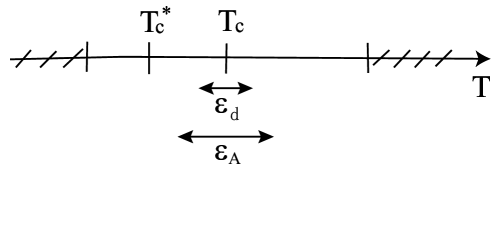
Figure 1: Schematic depiction of the relative magnitude of the critical regions, $\displaystyle\epsilon_{d}$ and $\displaystyle\epsilon_{A}$. Here $\displaystyle T_{c}$ is the critical temperature for the second order transition in the mean-field approximation, and $\displaystyle T_{c}^{*}$ the critical temperature of the first order transition induced by gauge-field fluctuations, derived below. In the hatched region where $\displaystyle|T-T_{c}|>T_{c}$, the Ginzburg-Landau expansion in terms of the order parameter is not justified.

Let us briefly summarize the results obtained in this section. For a type I color superconductor, as realized in the high density region, gluon fluctuations give the dominant correction to the free energy. As we show in the next section, in the one-loop approximation these fluctuations change the order of the phase transition from second to first, and modify the critical temperature from $\displaystyle T_{c}$ to $\displaystyle T_{c}^{*}$. If the relative shift of the critical temperature $\displaystyle(T_{c}^{*}-T_{c})/T_{c}$ is well outside the critical region dictated by Eqs. (15) and (16), the Gaussian approximation is consistent. This situation is quite analogous to the first order transition in type I metallic superconductor HLM .

On the other hand, in a type II color superconductor, which may be realized in the low density region for $\displaystyle T_{c}$ comparable to $\displaystyle\mu$, scalar fluctuations are not at all negligible. Furthermore, the Gaussian approximation becomes highly questionable. A renormalization group analysis with an $\displaystyle\epsilon$ expansion shows that, even without gauge fields, scalar fluctuations alone induce a first order transition in an $\displaystyle SU(n)\times SU(n)$ model with $\displaystyle n\geq 3$ PAT81 . Our model falls in this category when the coupling of the gauge field with the diquark condensate is neglected. A further complication for type II color superconductors is that the non-Abelian self-coupling of the gauge field may not be negligible, namely, the second condition Eq. (17) also becomes questionable at low densities. The non-Abelian coupling may change the order of the transition, as discussed in PIS00 , but that problem is beyond the scope of this paper.

The phase diagram in the ($\displaystyle\beta_{1},\beta_{2}$) plane implied by the GL free energy Eq. (1) is given in IB-I at the mean-field level without gauge fields. Once we take into account fluctuations of the order-parameter and the gauge fields, we need to consider the phase structure in the four dimensional ($\displaystyle\beta_{1},\beta_{2},\kappa_{T},\alpha_{s}$) space. Figure 2 shows its projection onto the two-dimensional ($\displaystyle\beta,\alpha_{s}$) space with $\displaystyle\beta\equiv\beta_{1}=\beta_{2}=3\kappa_{T}$. The CFL phase in the weak coupling limit lies in this reduced space (see the Appendix).

The solid line in the figure is the boundary separating type I and type II color superconductivity, characterized by $\displaystyle\kappa=1$ in Eq. (18). For the Gaussian approximation for the gauge fields to be reliable, $\displaystyle 2\alpha_{s}/\pi$ should be smaller than $\displaystyle 1$, Eq. (17). Therefore, within the shaded region in the figure, the one-loop approximation taking into account only the gauge field is reliable for studying effects of thermal fluctuations. The dashed line in the figure shows the relation between $\displaystyle\alpha_{s}$ and $\displaystyle\beta$ (both functions of $\displaystyle\mu$) in weak coupling, as obtained from the formulas in the Appendix. The weak coupling regime is well within the shaded area.

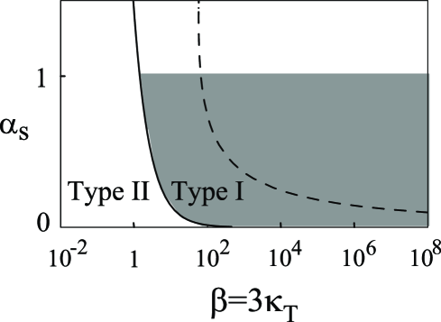
Figure 2: The phase structure in the two-dimensional ($\displaystyle\beta,\alpha_{s}$) space. The solid line, characterized by $\displaystyle\kappa=1$, is the boundary between type I (right side) and type II (left side) superconducting behavior. The dashed line shows $\displaystyle\alpha_{s}$ as a function of $\displaystyle\beta$, calculated in weak coupling. The loop expansion for gauge field fluctuations is valid in the shaded area.

In Fig. 3, we show $\displaystyle\kappa$ calculated in weak coupling, Eq. (19), as a function of the baryon chemical potential. The dependences of $\displaystyle\mu$ on $\displaystyle T_{c}$ and $\displaystyle\alpha_{s}$ are taken from the weak coupling results in the Appendix. The figure indicates that $\displaystyle\kappa\ll 1$ (type I superconductivity) is satisfied not only at high density but also at moderate densities, to the extent that one can rely on the extrapolation using the weak coupling formulas.

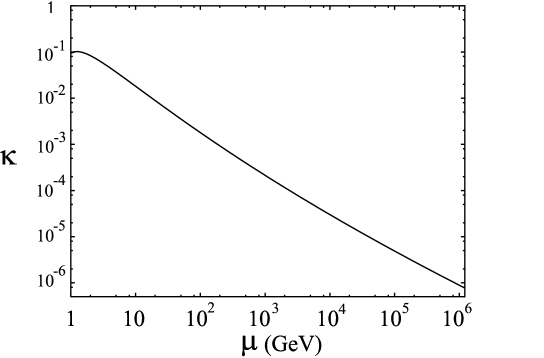
Figure 3: The parameter $\displaystyle\kappa$ calculated as a function of $\displaystyle\mu$ in the weak coupling approximation, Eq. (19).

III First order transition induced by gauge field

In this section we assume a type I color superconductor and evaluate the free energy of the CFL and IS states up to one-loop order, taking into account gauge field, but not scalar field, fluctuations. The free energy difference between the superfluid and normal phases, $\displaystyle F_{\rm eff}(d)$, in this approximation reads, in the Coulomb gauge,

$$\displaystyle F_{{\rm eff}}(d) \displaystyle= \displaystyle S(d)+\frac{1}{2}~{}\mbox{ln det}\left(\frac{\partial^{2}S}{\partial{\bf A}^{\alpha}\partial{\bf A}^{\beta}}\right)-F_{{\rm eff}}(d=0)$$ (22)

$$\displaystyle= \displaystyle S(d)+\frac{1}{2}~{}2T\sum_{\alpha}\int_{|{\bf k}|<T_{c}}\frac{d^{3}k}{(2\pi)^{3}}\{{\rm ln}~{}[k^{2}+(m_{A})_{\alpha\alpha}^{2}]-{\rm ln}~{}k^{2}\}$$

$$\displaystyle= \displaystyle S(d)+T\sum_{\alpha}\left[a_{2}(m_{A})_{\alpha\alpha}^{2}-a_{3}(m_{A})_{\alpha\alpha}^{3}+a_{4}(m_{A})_{\alpha\alpha}^{4}\right],$$

with

$$a_{2}=\frac{T_{c}}{2\pi^{2}},\ \ a_{3}=\frac{1}{6\pi},\ \ a_{4}=\frac{1}{4\pi^{2}T_{c}}.$$ (23)

We have included the two degrees of freedom associated with the polarization of the gauge fields in the Coulomb gauge. The high-momentum cutoff of the loop integral $\displaystyle\Lambda$, which sets the scale of the three-dimensional effective theory, is taken to be $\displaystyle T_{c}$, as discussed in the preceding section. The $\displaystyle m_{A}$, the non-zero Meissner masses listed in Table 1, are proportional to $\displaystyle d$, which here is a variational parameter determined by minimizing $\displaystyle F_{{\rm eff}}$ in the above formula. In evaluating the integral we have used the expansion in terms of $\displaystyle m/\Lambda=m/T_{c}$:

$$\displaystyle f(m)=\int_{|{\bf k}|<\Lambda}\frac{d^{3}k}{(2\pi)^{3}}\log\left(\frac{k^{2}+m^{2}}{k^{2}}\right)=\int_{0}^{m^{2}}dM^{2}\int_{|{\bf k}|<\Lambda}\frac{d^{3}k}{(2\pi)^{3}}\frac{1}{k^{2}+M^{2}}$$

$$\displaystyle=\frac{\Lambda}{2\pi^{2}}m^{2}-\frac{1}{6\pi}m^{3}+\frac{1}{4\pi^{2}\Lambda}m^{4}+{\cal O}(m^{6}).$$ (24)

The expansion is well convergent for $\displaystyle m_{A}\ll T_{c}$, corresponding to the condition Eq. (16). However, this is not necessarily a good expansion for $\displaystyle m_{A}\sim T_{c}$, which is realized at the critical point of first order transition as we shall see in Secs. III A and III B.

By setting $\displaystyle m=m_{d}$ in Eq. (III), we can roughly estimate the energy contribution from diquark fluctuations. This equation also allows us to see the reason why $\displaystyle\kappa$, introduced in the previous section, measures the relative importance of diquark and gauge field fluctuations in the free energy. At each order of the expansion of $\displaystyle F_{\rm eff}(d)$ in terms of $\displaystyle d$, the dominant contribution comes from the modes with largest mass. [Note that the energy scale entering Eq. (22), $\displaystyle T_{c}m_{d,A}^{3}$, can be regarded as the unit of thermal energy $\displaystyle\sim T$ times the number density, $\displaystyle\sim m_{d,A}^{3}$, of modes of mass $\displaystyle m_{d,A}$.] For the type I case, $\displaystyle\kappa=m_{d}/m_{A}\ll 1$, which indicates that the gauge field fluctuations dominate over diquark field fluctuations. One can also see from Eq. (III) that the massless modes in Table I do not contribute to the free energy difference $\displaystyle F_{\rm eff}$.

As we have discussed in the previous section and is easily seen by comparing Eqs. (22) and (13), the integral of the gauge field fluctuation $\displaystyle\langle{\bf A}^{2}\rangle$ with respect to $\displaystyle m_{A}^{2}$ leads precisely to the one-loop correction to the free energy. In particular, the term proportional to $\displaystyle a_{2}$ in Eq. (22) decreases the critical temperature of the second order transition since it is proportional to $\displaystyle d^{2}$ with a positive coefficient. On the other hand, the term proportional to $\displaystyle a_{3}$ drives the first order transition because it has a cubic structure $\displaystyle d^{3}$ with a negative coefficient. This is indeed the mechanism of the first order transition induced by thermal photons, first pointed out in HLM in the context of the type I metallic superconductors.

In dense QCD, Bailin and Love have previously discussed the first order transition induced by thermal gluons in two-flavor color superconductors BL . Considering only the terms proportional to $\displaystyle a_{2}$ and $\displaystyle a_{3}$, they concluded that the transition is strongly first order at high density. Furthermore, the strength of the first order transition grows as $\displaystyle\mu$ increases in their result [e.g., Eq. (4.100) in BL ]. On the contrary, as we show below, the strong first order transition induced by the $\displaystyle a_{3}$ term is substantially tamed by the consistent inclusion of the $\displaystyle a_{4}$ term for both CFL and IS orderings. As a consequence, the first order transition becomes weaker with increasing density, in contrast to the conclusion of BL .

III.1 Free energy of the CFL state

In this section, we show explicitly the one-loop free energy and the critical temperature of the first order transition $\displaystyle T_{c}^{*}$ for the CFL phase. If we use the CFL form in Eq. (6) and the Meissner masses in Table 1, the free energy $\displaystyle F_{\rm eff}(d)$ in Eq. (22) reads

$$\displaystyle F_{{\rm eff}}(d) \displaystyle= \displaystyle 3{\tilde{\alpha}}d^{2}-qd^{3}+rd^{4},$$ (25)

with

$$\displaystyle 3{\tilde{\alpha}}d^{2} \displaystyle= \displaystyle 3\bar{\alpha}d^{2}+8Ta_{2}m_{A}^{2}=\left[3\bar{\alpha}+\frac{TT_{c}}{\pi^{2}}\left(32\pi\kappa_{T}\alpha_{s}\right)\right]d^{2},$$ (26)

$$\displaystyle qd^{3} \displaystyle= \displaystyle 8Ta_{3}m_{A}^{3}=\left[\frac{8\sqrt{2}}{3}\frac{T}{\pi}\left(4\pi\kappa_{T}\alpha_{s}\right)^{{3}/{2}}\right]d^{3},$$ (27)

and

$$\displaystyle rd^{4} \displaystyle= \displaystyle 3(3\beta_{1}+\beta_{2})d^{4}+8Ta_{4}m_{A}^{4}=\left[3(3\beta_{1}+\beta_{2})+\left(\frac{T}{T_{c}}\right)128\kappa_{T}^{2}\alpha_{s}^{2}\right]d^{4}.$$ (28)

Here, $\displaystyle m_{A}=(2\kappa_{T})^{1/2}g|d|$ is the Meissner mass in the CFL phase.

As we have already mentioned, the effects of gauge fluctuations are threefold: First, they increase the size of the quadratic ($\displaystyle d^{2}$) terms. This increase implies that thermal fluctuations tend to make the superconducting phase less energetically favorable. Second, we find a cubic term with a negative coefficient, $\displaystyle-q$, which favors the superconducting phase. Furthermore, the second-order transition found in mean-field theory turns into a first order one due to this term, independent of the magnitude of $\displaystyle\mu$. Finally, we find a positive correction to the quartic term from the fluctuations. Like the correction to the quadratic term, this term acts against the superconducting phase. The sum of these three corrections leads to a first order transition which is significantly stronger than in a metallic superconductor, but is much weaker than that claimed in BL , where the quartic correction was neglected.

For later convenience, we define a “renormalized” critical temperature $\displaystyle T^{\prime}_{c}$ at which the quadratic term in Eq. (25) vanishes, $\displaystyle\tilde{\alpha}=0$. (Note that the critical temperature at the tree level, $\displaystyle T_{c}$, has been defined through $\displaystyle\bar{\alpha}=0$.) Then,

$$\displaystyle\frac{T^{\prime}_{c}}{T_{c}} \displaystyle= \displaystyle\left(1+\frac{T_{c}^{2}}{\alpha_{0}}\frac{32\kappa_{T}\alpha_{s}}{3\pi}\right)^{-1},$$ (29)

$$\displaystyle\tilde{\alpha} \displaystyle= \displaystyle\alpha_{0}\frac{T-T^{\prime}_{c}}{T^{\prime}_{c}}\equiv\alpha_{0}t^{\prime}.$$ (30)

The decrease of the renormalized critical temperature from the mean-field value ($\displaystyle T^{\prime}_{c}<T_{c}$) is consistent with the fact that the contribution of the fluctuations to the quadratic term makes the superconducting state less favorable.

On the other hand, the true critical temperature, $\displaystyle T_{c}^{*}$, of the first order transition is the temperature where the free energy has two degenerate minima, $\displaystyle d=0$ and $\displaystyle d=d^{*}\neq 0$. Since $\displaystyle F_{\rm eff}(0)=0$ by definition, this implies that $\displaystyle F_{\rm eff}(d^{*})=\partial F_{\rm eff}(d^{*})/\partial d^{*}=0$ is satisfied at $\displaystyle T=T_{c}^{*}$. Thus we find

$$\displaystyle\frac{T_{c}^{*}}{T^{\prime}_{c}} \displaystyle= \displaystyle 1+\frac{q^{2}}{12\alpha_{0}r},$$ (31)

$$\displaystyle d^{*} \displaystyle= \displaystyle\frac{q}{2r}.$$ (32)

The cubic term $\displaystyle-qd^{3}$ in the free energy, which tends to stabilize the superconducting phase, increases the critical temperature of the first order transition from $\displaystyle T^{\prime}_{c}$ as seen in Eq. (31). Thus the ratio $\displaystyle T_{c}^{*}/T^{\prime}_{c}$ is a measure of the strength of first order transition induced by the thermal gluons. One may also define other measures such as the jump of the diquark condensate at $\displaystyle T=T_{c}^{*}$ relative to its $\displaystyle T=0$ value, $\displaystyle d^{*}/d_{0}$, where $\displaystyle d_{0}=d(T=0)$.

Using the weak coupling formulas for $\displaystyle\beta_{i}$ and $\displaystyle\kappa_{T}$ in the Appendix, we find the following estimates of the above quantities at high density:

$$\displaystyle p \displaystyle\equiv \displaystyle\frac{3\alpha_{0}r}{q^{2}}\simeq\frac{81\pi}{14\zeta(3)\alpha_{s}},$$ (33)

$$\displaystyle\frac{T^{\prime}_{c}}{T_{c}} \displaystyle\simeq \displaystyle\left(1+\frac{9}{2\pi^{2}p}\right)^{-1},\ \ \ \frac{T_{c}^{*}}{T^{\prime}_{c}}\simeq 1+\frac{1}{4p},$$ (34)

$$\displaystyle d^{*} \displaystyle\simeq \displaystyle\pi^{5/2}\left(\frac{6}{7\zeta(3)}\right)^{1/2}\frac{T_{c}^{2}}{\mu\sqrt{\alpha_{s}}},$$ (35)

$$\displaystyle\frac{d^{*}}{d_{0}} \displaystyle\simeq \displaystyle\frac{e^{\gamma}\pi^{3/2}}{10}\left(\frac{6}{7\zeta(3)}\right)^{1/2}\frac{1}{\sqrt{\alpha_{s}}}\left(\frac{T_{c}}{100~{}{\rm MeV}}\right)\left(\frac{1~{}{\rm GeV}}{\mu}\right)\sim 0.3\kappa,$$ (36)

where we have used the mean-field relation $\displaystyle d_{0}=(\pi/e^{\gamma})T_{c}$ with $\displaystyle\gamma$ being Euler’s constant.

In Fig. 4(a) we compare the ratio $\displaystyle T^{\prime}_{c}/T_{c}$, $\displaystyle T_{c}^{*}/T^{\prime}_{c}$, and $\displaystyle T_{c}^{*}/T_{c}$ as functions of the baryon chemical potential $\displaystyle\mu$, with the weak coupling parameters of the Appendix. Note that $\displaystyle T_{c}^{*}$ is always smaller than $\displaystyle T_{c}$,

$$\displaystyle\frac{T_{c}^{*}}{T_{c}}-1\sim-\frac{\alpha_{s}}{10^{2}}.$$ (37)

In Fig. 4(b), the jump of the order parameter at the critical point, $\displaystyle{d^{*}}/{d_{0}}$, is shown as a function of $\displaystyle\mu$. The jump is at most a few percent for $\displaystyle\mu>1$ GeV, but is much larger than that expected in type I metallic superconductors (see below). Also, one finds that the first order transition becomes weaker logarithmically as $\displaystyle\mu$ increases, and approaches a second order transition at $\displaystyle\mu=\infty$. As noted above, this is in contrast to the result of BL in which the first order transition becomes strong as $\displaystyle\mu$ increases. Such behavior is unreasonable because the coupling of gluons and diquarks becomes weak at high density due to the asymptotic freedom. As we have already discussed, the discrepancy between our result and that in BL originates from the fact that thermal corrections to the quartic term in the free energy were not taken into account in BL . As we approach the baryon density close to that at the confinement-deconfinement transition, $\displaystyle\mu\sim 1$ GeV, the fluctuations of the scalar field as well as the non-Abelian interactions of the gluons neglected in our calculation become important. Therefore the results shown in Figs. 4(a,b) may be modified qualitatively in this region. Elucidating the super-to-normal transition in the low density region remains an interesting open question.

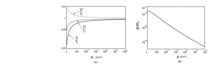
Figure 4: (a) The ratio of three critical temperatures, $\displaystyle T^{\prime}_{c}$/$\displaystyle T_{c}$ (solid line), $\displaystyle T_{c}^{*}$/$\displaystyle T_{c}$ (dashed line) and $\displaystyle T_{c}^{*}$/$\displaystyle T^{\prime}_{c}$ (dotted line). (b) The jump of the diquark condensate at $\displaystyle T=T_{c}^{*}$ relative to its $\displaystyle T=0$ value; $\displaystyle{d^{*}}/{d_{0}}$ as functions of the baryon chemical potential $\displaystyle\mu$ in the CFL phase. Weak coupling values for $\displaystyle\beta_{i}$ and $\displaystyle\kappa_{T}$ are used.

It is instructive to compare the strength of the present first-order transition with that of type I metallic superconductors. In the latter case, one finds an extremely weak first-order transition: $\displaystyle(T_{c}^{*}-T_{c}^{{}^{\prime}})/T_{c}^{{}^{\prime}}\sim\alpha^{3}(E_{F}/T_{c})^{2}(E_{F}/m)^{3/2}\sim 10^{-6}$ HLM ; BL . $\displaystyle E_{F}$ is the electron Fermi energy ($\displaystyle E_{F}=p_{F}^{2}/2m$), $\displaystyle m$ is the electron mass and $\displaystyle\alpha=e^{2}/4\pi$ is the electromagnetic fine structure constant. Major differences from the case of massless color superconductivity are the presence of a small factor $\displaystyle E_{F}/m$ and the small coupling constant. Note that in the metallic case, the thermal photon correction to the quartic term in the GL free energy divided by the corresponding mean-field value is $\displaystyle{\cal O}[\alpha^{2}(E_{F}/T_{c})^{2}(E_{F}/m)]$, which is the same order with or even smaller than unity. In contrast, thermal gluon fluctuations in the weak-coupling color superconductors dominate the quartic term [see Eq. (28)]. This is the reason why in the metallic case the shift $\displaystyle(T_{c}^{*}-T_{c}^{{}^{\prime}})/T_{c}^{{}^{\prime}}$ involves such a high power, $\displaystyle\alpha^{3}$, compared with only $\displaystyle g^{2}$ for color superconductivity.

Let us now discuss the reliability of the first order phase transition obtained here in weak coupling, from the point of view of the critical region examined in Sec. II.2. The first inequalities in Eqs. (15) and (16) can be interpreted as conditions for the size of $\displaystyle T-T_{c}$, or alternatively as conditions for the size of $\displaystyle d$; if $\displaystyle T_{c}^{*}-T_{c}$ or $\displaystyle d^{*}$ is very small, critical fluctuations are not negligible and one cannot trust the result of the one-loop approximation. In the case of weak coupling, $\displaystyle t^{*}\equiv|T_{c}^{*}-T_{c}|/T_{c}\simeq 10^{-2}\alpha_{s}$ from Eq. (37); in addition $\displaystyle T_{c}/\mu\ll 1$. Therefore, the conditions given in Eqs. (21) and (20), $\displaystyle t^{*}\gg\epsilon_{A,d}$, are well satisfied, and the critical temperature of the first order transition is outside the critical region of the diquark and gauge fluctuations. Also, by substituting $\displaystyle d^{*}$ in Eq. (35) into the first inequalities in Eqs. (15) and (16), one finds the conditions $\displaystyle\alpha_{s}/\beta\ll 1.6~{}\pi^{5}$ and $\displaystyle\alpha_{s}\ll\pi^{2}/6$, which should be satisfied for the effective three-dimensional approach to be valid. They are, in fact, well satisfied, insofar as the couplings stay in the shaded region in Fig. 2.

III.2 Free energy of the IS state

The analysis of the IS state is similar to that of the CFL state. The free energy in the one-loop approximation becomes

$$\displaystyle F_{\rm eff}(d)={\tilde{\alpha}}d^{2}-qd^{3}+rd^{4},$$ (38)

with

$$\displaystyle{\tilde{\alpha}}d^{2} \displaystyle= \displaystyle\bar{\alpha}d^{2}+Ta_{2}\left(4m_{A}^{2}+m_{\bar{A}}^{2}\right)=\left[\bar{\alpha}+\frac{TT_{c}}{\pi^{2}}\left(\frac{32\pi\kappa_{T}\alpha_{s}}{3}\right)\right]d^{2},$$ (39)

$$\displaystyle qd^{3} \displaystyle= \displaystyle Ta_{3}\left(4m_{A}^{3}+m_{\bar{A}}^{3}\right)=\left[\frac{T}{\pi}\left(\frac{2}{3}+\frac{4}{9\sqrt{3}}\right)\left(4\pi\kappa_{T}\alpha_{s}\right)^{{3}/{2}}\right]d^{3},$$ (40)

$$\displaystyle rd^{4} \displaystyle= \displaystyle(\beta_{1}+\beta_{2})d^{4}+Ta_{4}\left(4m_{A}^{4}+m_{\bar{A}}^{4}\right)=\left[(\beta_{1}+\beta_{2})+\frac{208}{9}\left(\frac{T}{T_{c}}\right)\kappa_{T}^{2}\alpha_{s}^{2}\right]d^{4}.$$ (41)

Here, $\displaystyle m_{A}$ and $\displaystyle m_{\bar{A}}$ are the Meissner masses, Table 1:

$$\displaystyle m_{A}^{2} \displaystyle= \displaystyle\kappa_{T}g^{2}d^{2}~{}~{}~{}~{}(\rm{4~{}components}),$$ (42)

$$\displaystyle m_{\bar{A}}^{2} \displaystyle= \displaystyle\frac{4}{3}\kappa_{T}g^{2}d^{2}~{}~{}~{}(\rm{1~{}component}).$$ (43)

If the global minimum of the mean-field theory is in the IS state, that is, the parameters $\displaystyle\beta_{1},\beta_{2}$ satisfy $\displaystyle-\beta_{1}<\beta_{2}<0$ (as shown in Fig. 1 of IB-I ), the effective potential in the mean field approximation yields a second order transition to the normal phase, and in the one-loop approximation, a first order transition. The renormalized temperature, $\displaystyle T_{c}^{{}^{\prime}}$, the critical temperature of the first order transition, $\displaystyle T_{c}^{*}$, and order parameter, $\displaystyle d^{*}$, at the minimum of the free energy are calculated as before:

$$\displaystyle\frac{T^{\prime}_{c}}{T_{c}} \displaystyle= \displaystyle\left(1+\frac{T_{c}^{2}}{\alpha_{0}}\frac{32\kappa_{T}\alpha_{s}}{3\pi}\right)^{-1},\ \ \ \frac{T_{c}^{*}}{T_{c}^{{}^{\prime}}}=1+\frac{q^{2}}{4\alpha_{0}r},$$ (44)

$$\displaystyle d^{*} \displaystyle= \displaystyle\frac{q}{2r}.$$ (45)

The relation, $\displaystyle T_{c}^{*}/T_{c}<1$, is also satisfied in this case. Since some of $\displaystyle m_{d}^{2}$’s in Table 1 are negative in the weak coupling ($\displaystyle\beta_{1}=\beta_{2}>0$), IS ordering is unstable against scalar fluctuations and decays into CFL ordering at high densities. This result is consistent with the result in Ref. IB-I where the comparison of the free energy between the IS and CFL orderings is made. As found from such comparison, the IS state is not in a local minimum when the CFL state is in the energy minimum. Nevertheless, the above formulas are relevant at finite temperature where the unlocking transition from CFL to IS ordering takes place due to the effect of the strange-quark mass, $\displaystyle m_{s}$ IB-I ; abuki .

IV Summary

In this paper we have studied the effect of thermal fluctuations of diquarks and the gluons on the superconducting-to-normal state phase transition in a three-flavor color superconductor. For this purpose, we adopted the Ginzburg-Landau free energy in three-spatial dimensions. Although the phase transition of this model is second order in the mean-field approximation for coupling constants near those in weak coupling, it can be turned into a first order transition either by the thermal fluctuations of the scalar diquark field, or the gluon gauge field near the critical point.

The relative importance of these two types of fluctuations is controlled by $\displaystyle\kappa$, the ratio of the masses of the scalar field and the gluon just below the critical temperature; $\displaystyle\kappa$ is also the Ginzburg-Landau parameter that differentiates type I and type II color superconductors. In the high density regime where the weak coupling approximation is valid, we find that the system is type I and gauge fluctuations dominate over scalar fluctuations.

After evaluating the size of the critical region, outside of which the one-loop approximation is a reasonable approximation, we calculate the one-loop correction to the free energy from the thermal gluons in a type I color superconductor. The transition to color superconductivity becomes first order due to the induced cubic term in the GL free energy, which is similar to the case of the type I metallic superconductors HLM .

The strength of the first phase transition can be characterized by quantities such as the change of the critical temperature from its tree-level value, and the jump of the order parameter at the critical point. They indicate that the first order transition weakens with increasing baryon density. This behavior, which is quite reasonable in the sense that gluonic corrections are suppressed by $\displaystyle\alpha_{s}$ in weak coupling, is in sharp contrast to that found for two-flavor color superconductivity in BL . The difference stems from the fact that one needs to take into account not only the cubic term of the order parameter (which strengthens the first order transition) but also thermal corrections to the quartic term (which suppresses the first order transition) to obtain a consistent result. Since the Ginzburg-Landau free energy has an intrinsic spatial cutoff scale $\displaystyle\Lambda^{-1}$, which is of order the size of the diquark ($\displaystyle\sim T_{c}^{-1}$), such a correction to the quartic term is an inevitable consequence of the three-dimensional effective theory. We also find that the critical temperature of the first order transition, $\displaystyle T_{c}^{*}$, is always lower than the $\displaystyle T_{c}$ of the second order transition in the mean-field approximation.

Our general considerations in this paper for a type I superconductor are valid insofar as the parameters in the Ginzburg-Landau free energy stay in the shaded area in Fig. 2, which corresponds to the high density region. On the other hand, in the low density, strong coupling region, not only scalar fluctuations but also non-Abelian interactions among thermal gluons are not negligible. Anti-quark pairing and the non-perturbative running of $\displaystyle\alpha_{s}$ at low momentum are also not negligible at low density AHI . These effects may change the nature of the phase transition at low density from that realized at high densities. Lattice simulations of the $\displaystyle SU(3)_{c}\times SU(3)_{L+R}\times U(1)_{B}$ sigma model + $\displaystyle SU(3)_{c}$ gauge field introduced in the present paper would be a good starting point to analyze the phase structure in the strong coupling region. Furthermore, the strange quark mass plays an important role in the unlocking transition from the CFL state to the IS state.

APPENDIX: ASYMPTOTIC VALUES OF THE COUPLING CONSTANTS

In this paper, we use $\displaystyle T_{c}$ calculated in finite temperature perturbation theory in the normal phase brown :

$$\displaystyle T_{c}=2\frac{e^{\gamma}}{\pi}256\pi^{4}\left(\frac{2}{N_{f}g^{2}}\right)^{5/2}e^{-(\pi^{2}+4)/8}\ ~{}\frac{\mu}{3}~{}{\rm exp}\left(-\frac{3\pi^{2}}{\sqrt{2}g}\right)$$ (46)

$$\displaystyle\alpha_{s}=\frac{g^{2}}{4\pi}=\frac{6\pi}{(33-2N_{f})\ln[\mu/(3\Lambda_{\rm QCD})]},$$ (47)

where $\displaystyle{e^{\gamma}}/{\pi}\sim 0.57$ and $\displaystyle\Lambda_{\rm QCD}$ for $\displaystyle N_{f}=3$ is taken to be 200 MeV.

The parameters in Eq. (1) as a function of $\displaystyle T_{c}$ and $\displaystyle\mu$ (baryon chemical potential) at asymptotically high densities, which were calculated from the finite temperature weak coupling gap equation in Refs. IB-I ; IB-III , are

$$\displaystyle{\bar{\alpha}}=4N(\mu/3)\ln\left(\frac{T}{T_{c}}\right),$$ (48)

$$\displaystyle\beta_{1}=\beta_{2}=3\kappa_{T}=\frac{7\zeta(3)}{8(\pi T_{c})^{2}}N(\mu/3),$$ (49)

$$\displaystyle N(\mu/3)=\frac{1}{2\pi^{2}}\left(\frac{\mu}{3}\right)^{2},$$ (50)

with the zeta function $\displaystyle\zeta(3)=1.2020\cdots$.

References

- (1) K. Rajagopal and F. Wilczek, in At the Frontier of Particle Physics/Handbook of QCD, edited by M. Shifman (World Scientific, Singapore, 2001); M.G. Alford, Annu. Rev. Nucl. Part. Sci. 51, 131 (2001).
- (2) D. Bailin and A. Love, Phys. Rep. 107, 325 (1984).
- (3) M. Iwasaki and T. Iwado, Phys. Lett. B 350, 163 (1995).
- (4) M. Alford, K. Rajagopal, and F. Wilczek, Phys. Lett. B 422, 247 (1998); R. Rapp, T.Schäfer, E. V. Shuryak, and M. Velkovsky, Phys. Rev. Lett. 81, 53(1998).
- (5) K. Iida and G. Baym, Phys. Rev. D 63, 074018 (2001); 66, 059903(E) (2002).
- (6) K. Iida and G. Baym, Phys. Rev. D 66, 014015 (2002).
- (7) K. Iida and G. Baym, Phys. Rev. D 65, 014022 (2002).
- (8) G. Baym, C. J. Pethick, and H. Monien, Nucl. Phys. A498, 313c (1989); G. Baym, H. Monien, C. J. Pethick, and D. G. Ravenhall, Phys. Rev. Lett. 64, 1867 (1990); Nucl. Phys. A525, 415c (1991).
- (9) D. T. Son, Phys. Rev. D 59, 094019 (1999).
- (10) R. D. Pisarski and D. H. Rischke, Phys. Rev. D 61, 074017 (2000).
- (11) B. I. Halperin, T.C. Lubensky, and S.-k. Ma, Phys. Rev. Lett. 32, 292 (1974).
- (12) G. Baym and G. Grinstein, Phys. Rev. D l5, 2897 (1977).
- (13) See, e.g. the recent paper, E. Bittner and W. Janke, Phys. Rev. Lett. 89, 130201 (2002).
- (14) R. D. Pisarski and D. H. Rischke, Phys. Rev. Lett. 83, 37 (1999).
- (15) A. J. Paterson, Nucl. Phys. B190, 188 (1981).
- (16) R. D. Pisarski, Phys. Rev. C 62, 035202 (2000).
- (17) I. Giannakis and H-c. Ren, Nucl. Phys. B669, 462 (2003).
- (18) N. Goldenfeld, Lectures on Phase Transitions and the Renormalization Group (Addison-Wesley, Reading, MA, 1992).
- (19) V. L. Ginzburg, Fiz. Tverd. Tela 2, 2031 (1960) [Sov. Phys. Solid State 2, 1824 (1961)].
- (20) H. Georgi, Weak Interactions and Modern Particle Theory (W.A. Benjamin, Menlo Park, CA, 1984).
- (21) V. L. Ginzburg and L. D. Landau, Zh. Eksp. Theor. Fiz. 20, 1064 (1950) [L.D. Landau Collected Papers(Pergamon Press, London, 1965), p. 546]; A.A. Abrikosov, Zh. Eksp. Teor. Fiz. 32, 1442 (1957) [Sov. Phys. JETP 5, 1174 (1957)].
- (22) M. G. Alford, J. Berges, and K. Rajagopal, Nucl. Phys. B558, 219 (1999); T. Schäfer and F. Wilczek, Phys. Rev. D 60 074014 (1999); H. Abuki, Prog. Theor. Phys. 110, 937 (2003).
- (23) H. Abuki, T. Hatsuda, and K. Itakura, Phys. Rev. D 65, 074014 (2002).
- (24) W. E. Brown, J.T. Liu, and H.-c. Ren, Phys. Rev. D 62, 054016 (2000).
- (25) M. Kitazawa, T. Koide, T. Kunihiro, and Y. Nemoto, Phys. Rev. D 65, 091504 (2002).