Hadronic contributions to $a_{\mu}$ below one GeV

Abstract

I present a method for evaluating the hadronic vacuum polarization contribution below 1 GeV to $a_{\mu}$ which relies on analyticity, unitarity and chiral symmetry, as well as on data. The main advantage is that in the region just above threshold, where data are either scarce or have large errors, these theoretical constraints are particularly strong, and therefore allow us to reduce the uncertainties with respect to a purely data–based evaluation. Some preliminary numerical results are presented as illustration of the method.

1 Introduction

The anomalous magnetic moment of the muon $a_{\mu}$ is now known experimentally to an extremely high precision [1], and can therefore be used as a thorough test of the standard model. The most uncertain and debated part of the standard model calculation of $a_{\mu}$ is the hadronic vacuum polarization contribution $a_{\mu}^{\rm hvp}$ . In order to make this test of the standard model a significant one, we need to make substantial progress in the evaluation of the hadronic contributions, and in particular of the leading one, $a_{\mu}^{\rm hvp}$ – which was precisely the scope of this Workshop. This contribution can be calculated in terms of another experimentally measured quantity, the cross section $e^{+}e^{-}\to$ hadrons, and any improvement in the measurement of this cross section is immediately reflected in $a_{\mu}^{\rm hvp}$ . Indeed many discussions at the Workshop concerned different possible ways to measure the $e^{+}e^{-}$ hadronic cross section, and have given us an overview of an impressive amount of experimental and theoretical work devoted to this problem. Given a set of data points at different center of mass energies for $\sigma(e^{+}e^{-}\to\mbox{hadrons})$, the evaluation of $a_{\mu}^{\rm hvp}$ amounts to the calculation of an integral of a function once one knows it at a discrete set of points. This problem is standard, and can be solved in different ways – the simplest of them being the use of the trapezoidal rule, as done, e.g. in Refs. [2, 3].

The use of the trapezoidal rule, or variants thereof, reduces the role of theory to an absolute minimum – the evaluation of $a_{\mu}^{\rm hvp}$ is done almost only with data. The role of theory cannot be reduced to zero because it is needed in the two extreme regions $s\sim 4M_{\pi}^{2}$ and $s\to\infty$. In the latter region one can make use of perturbative QCD, and in the former one of chiral perturbation theory (CHPT). Actually, CHPT cannot give a sharp numerical prediction for the pion vector form factor $F_{V}(s)$ (the dominating contribution below 1 GeV) close to threshold: it only predicts that the behaviour is very smooth, well approximated by a polynomial, whose coefficients are related to a few of the low energy constants of the chiral Lagrangian. The use of CHPT in this region amounts to an extrapolation of the data at somewhat higher energies down to threshold with a polynomial of low degree [2, 3].

My aim here is to show that not only close to threshold, but even up to 1 GeV the use of some theory is actually quite useful, especially because it allows one to reduce the uncertainty in $a_{\mu}^{\rm hvp}$ – and this region contributes the largest fraction of the total error. Theory in this case means some very general properties which we know the vector form factor $F_{V}(s)$ must satisfy: analyticity and unitarity. Combining these properties with chiral symmetry, which is relevant in the very low energy region, one can construct a representation which is very constraining for the form factor: the remaining little freedom can be fixed with the help of data as I illustrate in what follows.

2 Definition of $a_{\mu}^{\rm hvp}$ 

The leading hadronic contribution to $(g-2)_{\mu}$ is due to the hadronic vacuum polarization correction shown in Fig. 1.

Figure 1: Hadronic vacuum polarization contribution to $(g-2)_{\mu}$.

This contribution to $(g-2)_{\mu}$ is of order $\alpha^{2}$ and can be expressed in terms of the cross section $\sigma(e^{+}e^{-}\to\mbox{hadrons})$ evaluated to leading order in $\alpha$ [4]:

$$a_{\mu}^{\mbox{\tiny hvp}}=\left({\alpha m_{\mu}\over 3\pi}\right)^{2}\int_{4M_{\pi}^{2}}^{\infty}ds{\hat{K}(s)R^{(0)}(s)\over s^{2}}\,,$$ (1)

where $\hat{K}(s)$ is a known kernel, see e.g. [5], and

$$R^{(0)}(s)\equiv{\sigma^{(0)}(e^{+}e^{-}\to\mbox{hadrons})\over 4\pi\alpha^{2}/3s}\,,$$ (2)

where the superscript indicates that the cross section has to be taken to leading order in $\alpha$. At low energy $\sqrt{s}\leq 1$ GeV, the contribution of the two–pion state dominates the cross section

$$R^{(0)}(s)\simeq R^{\pi\pi}(s)={1\over 4}\left(1-4M_{\pi}^{2}/s\right)^{3/2}\left|F_{V}(s)\right|^{2}\,.$$ (3)

The latter, as shown, is given by the vector form factor of the pion (again to leading order in $\alpha$), which is the quantity we will now discuss.

3 The pion vector form factor

The pion vector form factor $F_{V}(s)$ is an analytic function of $s$ in the whole complex plane, with the exception of a cut on the real axis for $s\geq 4M_{\pi}^{2}$: approaching the real axis from above the form factor stays complex and can be described in terms of two real functions, its modulus and phase:

$$F_{V}(s)=|F_{V}(s)|e^{i\delta(s)}\,.$$ (4)

Omnès [6] has shown that analyticity relates the modulus and the phase, such that the whole function can be given in closed form in terms of its phase:

$$F_{V}(s)=P(s)\exp\left[\frac{s}{\pi}\int_{4M_{\pi}^{2}}^{\infty}dx\,\frac{\delta(x)}{x\,(x-s)}\right]\,,$$ (5)

where $P(s)$ is a polynomial which determines the behaviour of the function at infinity, or number and position of its zeros. In order to respect charge conservation $F_{V}(0)=1$, we set $P(0)=1$. The representation (5) makes it apparent that if one knows the phase on the cut and the zeros of the form factor one can calculate the form factor everywhere in the complex plane.

In the elastic region Watson’s theorem relates the phase of the vector form factor to the phase of the $\pi\pi$ scattering amplitude with the same quantum numbers, $I=\ell=1$:

$$\delta(s)=\delta_{1}^{1}(s)\quad\mbox{for}\quad s\leq s_{in}=16M_{\pi}^{2}\,.$$ (6)

While the inelastic threshold $\sqrt{s_{in}}=.56$ GeV appears to be rather low, inelastic contributions in this channel are known to become relevant only above the $K\bar{K}$ threshold. To an excellent approximation the phase of the vector form factor coincides with the $\pi\pi$ phase shift $\delta_{1}^{1}$ up to 1 GeV. The latter has been recently studied in the framework of Roy equations, first with no extra input [7], and also in combination with chiral symmetry [8]. The upshot of these analyses is that $\delta_{1}^{1}$ is constrained to a remarkable degree of accuracy up to about 0.8 GeV. In our approach we make explicit use of these general properties of the vector form factor, and of our knowledge of the $\pi\pi$ phase shifts. Our strategy can be summarized in the following points:

1. we construct a convenient representation which automatically respects the properties of analyticity, unitarity and chiral symmetry;

2. we fix the free parameters which appear in this representation by fitting data;

3. we evaluate the integral (1) up to 1 GeV using our analytic representation of the form factor.

A similar strategy was also adopted in Ref. [9], but with a limited use of chiral symmetry.

4 A convenient representation of the vector form factor

As discussed above, the vector form factor in the low energy region is to a large extent dominated by the $\pi\pi$ phase shift $\delta_{1}^{1}$. Inelastic effects, which are small, but nonnegligible at the needed level of accuracy, will also be taken into account and parametrized in terms of a smooth function which has the correct analytic properties. In order to evaluate $a_{\mu}^{\rm hvp}$ we need the vector form factor to leading order in $\alpha$, i.e. with electromagnetic interactions switched off – our form factor $F_{V}$ does not include vacuum polarization corrections. To make the connection to the $\pi\pi$ phase determined in [8] it is also convenient to work in the isospin limit of strong interactions $m_{u}=m_{d}$. In the $\pi\pi$ scattering amplitude these isospin-violating effects only show up at order $(m_{u}-m_{d})^{2}$ and are negligible. In the form factor, however, they are linear in the quark mass difference, and moreover they are enhanced, in a certain energy region, by the small mass difference between the $\rho$ and $\omega$ mesons, which appears in the denominator. This enhanced isospin-violating effect cannot be neglected at the level of accuracy which we are working at. We are therefore going to represent the form factor as a product of three functions that account for the prominent singularities in the low energy region [10]:

$$F(s)=G_{1}(s)\cdot G_{2}(s)\cdot G_{\omega}(s)\,.$$ (7)

The first term is the Omnès factor that describes the cut due to $2\pi$ intermediate states:

$$G_{1}(s)=\exp\left\{\frac{s}{\pi}\int_{4M_{\pi}^{2}}^{\infty}\frac{dx\,\delta_{1}^{1}(x)}{x\,(x-s)}\right\}\,.$$ (8)

The phase $\delta_{1}^{1}$ which enters $G_{1}(s)$ is obtained with an updated version of the analysis in [8]: in solving Roy equations we need an input for the imaginary part of the various partial waves at and above 0.8 GeV. In [8] the input $I=\ell=1$ partial wave had been fixed with the CLEO data [11] on the vector form factor: the most important input parameter, the phase at $\sqrt{s_{0}}=0.8$ GeV had been taken equal to

$$\delta_{1}^{1}(s_{0})=(108.9\pm 2)^{\circ}\,.$$ (9)

Above that energy we had used the parametrization of Hyams et al. [12]. In the present work we leave $\delta_{1}^{1}(s_{0})$ and $\delta_{1}^{1}(s_{1})$, with $\sqrt{s_{1}}=1.15$ GeV (the upper limit of validity of the Roy equations), as free parameters and determine them by fitting data on the form factor. Once these input parameters are given, Roy equations and chiral symmetry fix uniquely the phase between these two points and all the way down to threshold, as illustrated in Fig. 2.

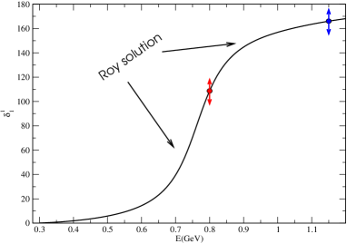
Figure 2: The $\pi\pi$ phase shift $\delta_{1}^{1}$: the value of the phase at the two (red and blue) dots are free and the Roy equations and chiral symmetry completely fix the phase everywhere else.

The phase shown in the plot corresponds to

$$\delta_{1}^{1}(s_{0})=109.5^{\circ}\qquad\delta_{1}^{1}(s_{1})=165.9^{\circ}$$ (10)

which are typical values we obtain in our fits, and in perfect agreement with the input phase used in [7]. The error which we get on $\delta_{1}^{1}(s_{0})$ is however about a factor two smaller than that in (9).

The function $G_{\omega}(s)$ contains the pole generated by $\omega$ exchange,

$$G_{\omega}(s) = 1+\epsilon\,\frac{s}{s_{\omega}-s}+\ldots$$

$$s_{\omega} = (M_{\omega}-\mbox{$\frac{1}{2}$}\,i\,\Gamma_{\omega})^{2}\,.$$ (11)

The pole term cannot stand by itself because it fails to be real in the spacelike region. We replace it by a dispersion integral with the proper behaviour at threshold, but this is inessential: the representation for $G_{\omega}(s)$ that we are using is (a) fully determined by the values of $\epsilon$, $M_{\omega}$ and $\Gamma_{\omega}$ and (b) in the experimental range, $|G_{\omega}(s)|$ is numerically very close to the magnitude of the pole approximation.

The function $G_{2}(s)$ represents the smooth background that contains the curvature generated by the singularities not acconted for by $G_{1}$ and $G_{\omega}$. We analyze this term by means of a conformal mapping. The $4\pi$ channel opens at $s_{in}=16\,M_{\pi}^{2}$, but phase space strongly suppresses the strength of the corresponding branch point singularity, which is of the form $(1-s_{in}/s)^{9/2}$. The transformation

$$z=\frac{\sqrt{s_{in}-s_{1}}\,-\sqrt{s_{in}-s}}{\sqrt{s_{in}-s_{1}}\,+\sqrt{s_{in}-s}}$$ (12)

maps the plane cut along $s>s_{in}$ onto the unit disk in the $z$-plane. It contains a free parameter $s_{1}$ – the value of $s$ that gets mapped into the origin. We find that if $s_{1}$ is taken negative and sufficiently far from the origin, the fit becomes insensitive to its specific value. We set $s_{1}=-1\,\mbox{GeV}^{2}$.

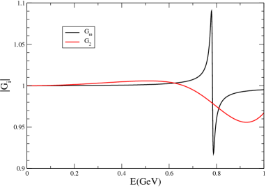
Figure 3: Typical shapes of the factors $G_{2}$ and $G_{\omega}$ that enter the vector form factor.

We approximate $G_{2}(s)$ by a polynomial in the variable $z$,

$$G_{2}(s)=1+\sum_{i=1}^{P}c_{i}\,(z^{i}-z_{0}^{i})\,,$$ (13)

where $z_{0}$ is the image of the point $s=0$. The terms involving $z_{0}$ ensure that the background does not modify the charge, $G_{2}(0)=1$. The condition that the branch point singularity has the form $(1-s_{in}/s)^{9/2}$ implies four constraints on the coefficients: if we want a nontrivial contribution from $G_{2}(s)$ we need at least a fifth–order polynomial. In the following we will vary $P$, the order of the polynomial, between $0$ and $8$. Both factors $G_{2}$ and $G_{\omega}$ are very small in the region up to 1 GeV, as illustrated in Fig. 3: only $G_{\omega}$ generates a 10% effect but only in a very narrow region around $M_{\omega}$, otherwise both give an effect at the few percent level. Notice that in principle $G_{2}$ may have zeros somewhere in the complex $s$ plane, as allowed by the general Omnès representation (5) – we make no assumptions on their position, nor on their number, if we vary $P$, and let the data choose where they should lie.

5 Numerical results

$P$	$\chi^{2}/$d.o.f.	$\chi^{2}_{\mathrm{CMD2}}$	$\chi^{2}_{\mathrm{NA7}}$	$10^{10}a_{\rho}$	$10^{10}a_{2M_{K}}$	$\langle r^{2}\rangle(\mbox{fm}^{2})$
0	84.9/83	43.6	43.7	$420.1\pm 2.1$	$489.5\pm 2.2$	$0.4254\pm 0.0020$
5	78.4/82	35.9	42.6	$423.8\pm 2.6$	$494.1\pm 2.7$	$0.4300\pm 0.0024$
6	78.1/81	36.0	42.2	$424.4\pm 2.8$	$494.7\pm 2.9$	$0.4339\pm 0.0051$
7	73.5/80	31.7	42.2	$423.4\pm 2.9$	$493.2\pm 3.0$	$0.4350\pm 0.0051$
8	73.5/79	31.6	42.2	$423.5\pm 5.7$	$493.4\pm 7.4$	$0.4347\pm 0.0052$

Table 1: Numerical results for fits to CMD-2 [13] and (spacelike) NA7 data [14]. The CMD-2 data used here do not contain vacuum polarization effects nor final state radiation. The errors given are purely statistical.

Our representation of the vector form factor involves three functions, each of which has free parameters which we pin down by fitting data. The free parameters at our disposal are the following:

• in $G_{1}$ we have two free parameters, the value of the phase $\delta_{1}^{1}$ at 0.8 and at 1.15 GeV;

• in $G_{2}$ we have $P-4$ free parameters, where $P$ is the degree of the polynomial in the conformal variable $z$. We will vary $P$ within a reasonable range of values, and see how the results depend on it;

• in $G_{\omega}$ we have in principle three free parameters, $\epsilon_{\omega}$, $M_{\omega}$ and $\Gamma_{\omega}$ – however, since the mass and width of the $\omega$ are rather well known from other experiments we fix them at the PDG values. We allow, however, the energy calibration (to which $G_{\omega}$ is very sensitive) to shift within the estimated experimental systematic uncertainty.

All in all we have $4+(P-4)$ free parameters, depending on the degree of the polynomial used to describe inelastic effects.

An example of our numerical results obtained by fitting the most recent CMD-2 data and the spacelike NA7 data [14] for values of $P$ between 0 and 8 is given in Table 1. The quantities denoted by $a_{\rho}$ and $a_{2M_{K}}$ correspond to the integral (1) cut off at 0.81 GeV and $2M_{K}$ respectively, whereas $\langle r^{2}\rangle$ is the square of the pion charge radius. It is worth stressing that the good fit obtained with $P=0$ shows how well the two–pion intermediate state alone describes the behaviour of the form factor both in the timelike and the spacelike region. The numerical results obtained in the first line can be considered as a theoretical prediction of $a_{\rho}$ based on the calculation of the $\pi\pi$ phase shift done in [8] (of course the results in that paper is also based on some experimental input). It is clear, however, that at the level of precision needed for $a_{\mu}^{\rm hvp}$ this prediction is not sufficiently precise and we must explicitly account for the inelastic effects encoded in $G_{2}$.

$10^{10}a_{\rho}$	$10^{10}a_{2M_{K}}$	$E_{max}^{e}/E_{max}^{\tau}$(GeV)	$\chi^{2}_{\mbox{\tiny CMD2}}$	$\chi^{2}_{\mbox{\tiny OLYA}}$	$\chi^{2}_{\mbox{\tiny ALEPH}}$	$\chi^{2}_{\mbox{\tiny CLEO}}$
421.5	—	.81/—	20.3(27)	14.1(26)	—	—
431.0	—	—/.81	—	—	8.1(10)	16.3(21)
427.2	—	.81/.81	21.1(27)	22.4(25)	11.0(10)	19.7(21)
427.4	497.7	.97/.81	38.2(43)	27.3(42)	12.0(10)	20.1(21)
427.7	501.0	.81/.97	22.0(27)	23.9(25)	12.3(16)	31.3(28)

Table 2: Results of simultaneous fit to $e^{+}e^{-}$ and $\tau$ data in different energy regions. The third column gives the maximal energy up to which the $e^{+}e^{-}$ or $\tau$ data are fitted. The first two rows concern fits done to either $e^{+}e^{-}$ or $\tau$ data. The number in brackets next to the $\chi^{2}$ value gives the number of data points fitted.

If we switch on the function $G_{2}$ and allow for one free parameter in it ($P=5$) we observe a sizeable improvement in the $\chi^{2}$, mainly in the part which comes from CMD-2 data – the addition of a further parameter ($P=6$) slightly improves the fit to the NA7 data. With $P=7$ we have again a sizeable decrease in $\chi^{2}_{\mbox{\tiny CMD2}}$, whereas going to $P=8$ brings no improvement anymore but leads to a substantial increase in the errors on all calculated quantities. Going to even higher values of $P$ does not make sense anymore, and it is reasonable to choose as final result the one with $P=7$, while the variation of the result with $P$ will be included in the final uncertainty, e.g. by taking the difference among the $P=6$ and $P=7$ results as theoretical uncertainty. These numbers are preliminary and given only for illustration purposes: the most important point to stress concerns the uncertainties, rather than the central values. A comparison to results obtained with the trapezoidal rule, like e.g. the recent update of Jegerlehner [5]

$$a_{\rho}=429.02\pm 4.95\,\mbox{ (stat.)}$$ (14)

shows that the reduction in the purely statistical error is substantial. Final results will be given in a forthcoming publication [15]. We plan to extend the analysis to other sets of data, like older $e^{+}e^{-}$ data (e.g. [16]), but also data on the weak vector form factor from $\tau$ decays [17, 11].

As is well known, the latter sets of data show a systematic deviation from the $e^{+}e^{-}$ ones, even after correction for known isospin violating effects [18]. One should stress that the calculation of these effects, although done on a sound theoretical basis, cannot be improved systematically: it is difficult to estimate the final theoretical uncertainty in the calculation of these corrections, and it is therefore not possible to exclude that the remaining discrepancy between $e^{+}e^{-}$ and $\tau$ data is actually due to an unaccounted isospin violating effect. Indeed this possibility (in particular a difference in mass and width between charged and neutral $\rho$ mesons) has been discussed at this Workshop [19] and in a recent publication [20].

One of the striking features of this discrepancy is that it has a peculiar energy dependence: as observed in [21], the two sets of data are in good agreement below about 0.8 GeV, but show a marked difference from that energy on. It is in fact possible to make a good fit to both sets of data if one limits oneself to the energy region below 0.8 GeV, as illustrated in Tab. 2. The first two rows give the results of the fits to either the $e^{+}e^{-}$ or the $\tau$ data: the outcome for $a_{\rho}$ shows a discrepancy of about 10 units, which is certainly larger than the error one would like to achieve in this determination. In the third row, however, it is shown that if one fits simultaneously all data sets one can still obtain a good $\chi^{2}$ for all data sets, and a value for $a_{\rho}$ which sits between the $e^{+}e^{-}$ and $\tau$ value, somewhat closer to the latter. The last two rows show that if one extends the fit region higher up only for one of the two sets of data, the result for $a_{\rho}$ remains stable, whereas the discrepancy in the value of $a_{2M_{K}}$ is reduced to about three units.

6 Conclusions

I have discussed a method of calculation of the low energy contribution to $a_{\mu}^{\rm hvp}$ which relies as much as possible on theory – in the form of analyticity, unitarity and chiral symmetry. These properties do constrain the vector form factor of the pion below 1 GeV quite strongly and can be used to safely interpolate between data. In particular, it is sufficient to have very precise data in the $\rho$ region to pin down the free parameters in the form factor and make a controlled extrapolation down to threshold. In this manner one can sizeably reduce the error in $a_{\mu}^{\rm hvp}$ coming from this energy region, where data are scarce and with larger errors. I have illustrated this with a few numerical examples and stressed, in particular, that because of the agreement between $e^{+}e^{-}$ and $\tau$ data below 0.8 GeV, one can give a stable prediction for the region below this energy. The analysis is still in progress, and final results will be given in a forthcoming publication [15].

In this Workshop we have heard of plans or ongoing efforts for measuring the pion vector form factor in several different ways, which means that in a few years time there will be several new sets of data to which this method can be applied. It will be extremely interesting to look at the picture that will emerge from these.

References

- [1] H. N. Brown et al. [Muon g-2 Collaboration], Phys. Rev. Lett. 86 (2001) 2227 [arXiv:hep-ex/0102017].
- [2] S. Eidelman and F. Jegerlehner, Z. Phys. C 67 (1995) 585 [arXiv:hep-ph/9502298].
- [3] M. Davier, S. Eidelman, A. Hocker and Z. Zhang, Eur. Phys. J. C 27 (2003) 497 [arXiv:hep-ph/0208177].
- [4] M. Gourdin and E. De Rafael, Nucl. Phys. B 10 (1969) 667.
- [5] F. Jegerlehner, arXiv:hep-ph/0310234.
- [6] R. Omnes, Nuovo Cim. 8 (1958) 316.
- [7] B. Ananthanarayan, G. Colangelo, J. Gasser and H. Leutwyler, Phys. Rept. 353 (2001) 207 [arXiv:hep-ph/0005297].
- [8] G. Colangelo, J. Gasser and H. Leutwyler, Nucl. Phys. B 603 (2001) 125 [arXiv:hep-ph/0103088].
- [9] J. F. De Trocóniz and F. J. Yndurain, Phys. Rev. D 65 (2002) 093001 [arXiv:hep-ph/0106025].
- [10] H. Leutwyler, arXiv:hep-ph/0212324.
- [11] S. Anderson et al. [CLEO Collaboration], Phys. Rev. D 61 (2000) 112002 [arXiv:hep-ex/9910046].
- [12] B. Hyams et al., Nucl. Phys. B 64 (1973) 134.
-
[13]
R. R. Akhmetshin et al. [CMD-2 Collaboration],
Phys. Lett. B 527 (2002) 161
[arXiv:hep-ex/0112031],
and arXiv:hep-ex/0308008 for a reanalysis of the same data. - [14] S. R. Amendolia et al. [NA7 Collaboration], Nucl. Phys. B 277 (1986) 168.
- [15] I. Caprini, G. Colangelo, F. Jegerlehner and H. Leutwyler, in preparation.
- [16] L. M. Barkov et al. [OLYA and CMD Collaborations], Nucl. Phys. B 256 (1985) 365.
- [17] R. Barate et al. [ALEPH Collaboration], Z. Phys. C 76 (1997) 15.
- [18] V. Cirigliano, G. Ecker and H. Neufeld, JHEP 0208 (2002) 002 [arXiv:hep-ph/0207310].
-
[19]
M. Davier, these proceedings,
F. Jegerlehner, these proceedings. - [20] S. Ghozzi and F. Jegerlehner, arXiv:hep-ph/0310181.
- [21] M. Davier, S. Eidelman, A. Hocker and Z. Zhang, arXiv:hep-ph/0308213.