Theoretical uncertainties on $\boldsymbol{\alpha_{s}}$ from event-shape variables in $\boldsymbol{{\rm e}^{+}{\rm e}^{-}}$ annihilations

Abstract:

The precision of measurements of the strong coupling constant using event-shape variables in ${\rm e}^{+}{\rm e}^{-}$ annihilations is limited by theoretical systematic uncertainties. The uncertainties are related to missing higher orders in the perturbative predictions for the event-shape distributions. A new method is presented for the assessment of theoretical uncertainties in $\alpha_{s}$. This method evaluates the systematic uncertainty of the parameter $\alpha_{s}$ from the uncertainty of the prediction for the distributions from which it is extracted. The perturbative uncertainties are calculated on a purely theoretical basis, without accessing measured distributions. The method is therefore especially suited for an unbiased combination of results from different observables or experiments. It is universal and can be applied to other processes like jet production in deep-inelastic $ep$ scattering or in hadron collisions.

1 Introduction

Studies of Quantum Chromodynamics in ${\rm e}^{+}{\rm e}^{-}$ annihilations have been carried out over more than 30 years at increasing centre-of-mass energies. Event-shape variables have proven to be key observables in both annihilation and deep-inelastic scattering processes. The understanding of perturbative and non-perturbative aspects of QCD has grown with the study of event shapes. While event shapes were first introduced to characterise global properties, it was soon realised that their distributions are sensitive to the strong coupling constant $\alpha_{s}$. The perturbative prediction for a generic infrared-collinear (IRC) safe event-shape variable $y$ can be computed to second order in $\alpha_{s}$,

$$\frac{1}{\sigma}\frac{d\sigma}{dy}=A(y)\frac{\alpha_{s}}{2\pi}+B(y)\left(\frac{\alpha_{s}}{2\pi}\right)^{2}\;,$$ (1)

with coefficient functions $A$ and $B$ obtained from integration of the ERT[1] matrix elements. Using this type of prediction, first determinations of $\alpha_{s}$ were performed at the PEP and PETRA colliders. In the era of the LEP experiments the calculations for certain classes of variables were improved by resumming leading and next-to-leading logarithmic terms (NLL). These calculations, matched to fixed-order expressions, enlarged the kinematic range of applicability for $\alpha_{s}$ extractions and reduced the systematic theoretical uncertainty. Recently, event-shape variables have also been used extensively to study non-perturbative power law corrections. It has been shown that hadronisation corrections, scaling with inverse powers of the momentum transfer $Q$ can be modelled with one or a few non-perturbative parameters [2]. These parameters can in turn be related to moments of an effective coupling at low scales, and have been extracted from the data [3].

At present measurements of $\alpha_{s}$ using event-shape variables and $\mathcal{O}(\alpha_{s}^{2})+$NLL resummed calculations are available at centre-of-mass energies between 22 GeV and 206 GeV. For illustration a selection of these measurements is shown in Fig. 1.

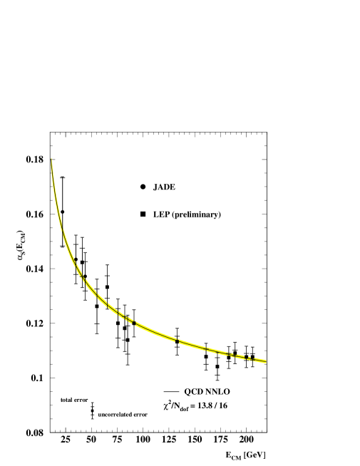
Figure 1: Measurements of $\alpha_{s}$ from event-shape variables as function of centre-of-mass energy.

New measurements re-analysing data from the JADE collaboration [4] were performed using a technique similar to that applied for a combined analysis by the LEP collaborations [5]. In particular, the same theoretical framework was used and at most of the energies a similar set of variables was combined. At almost all energies perturbative theoretical uncertainties dominate other systematic uncertainties, e.g. at $Q=M_{\rm Z}$ the perturbative uncertainty is $5\%$ and the quadratic sum of statistical, experimental and hadronisation uncertainties is $1.3\%$.

It is the objective of this note to examine ways of estimating the theoretical uncertainties and to propose a comprehensive and consistent method to combine different uncertainty estimates. In addition, the proposed method should allow the calculation of the uncertainty associated with a given measurement without using the data from which $\alpha_{s}$ is extracted. This is notably important for global combinations of various measurements, where a coherent procedure must be applied.

The origin of perturbative theoretical uncertainties is the truncation of the perturbative series at a given order of the coupling constant, whereby the truncated prediction acquires a dependence on the renormalisation scale.

To illustrate this point, a fully inclusive observable, the total hadronic cross section $\sigma({\rm e}^{+}{\rm e}^{-}\rightarrow{\rm q\bar{q}})$, is considered as an example for which third order $\mathcal{O}(\alpha_{s}^{3})$ calculations are available. The ratio $R_{\rm Z}$ of hadronic to leptonic widths at the Z boson resonance reads (with renormalisation scale $\mu=Q$) [6]

$$R_{\rm Z}=\frac{\Gamma({\rm Z^{0}\rightarrow hadrons})}{\Gamma({\rm Z^{0}\rightarrow leptons})}=R_{\rm EW}\sum_{n=0}^{3}c_{n}\left(\frac{\alpha_{s}}{\pi}\right)^{n}$$ (2)

with

$$R_{\rm EW}=19.934\;,\;\;c_{0}=1\;,\;\;c_{1}=1.045\;,\;\;c_{2}=0.94\;,\;\;c_{3}=-15\,,$$ (3)

One estimate of the theoretical uncertainty on $R_{\rm Z}$ is based on the size of the last term in the series, taking the difference between the full next-to-next-to-leading order (NNLO) prediction and the next-to-leading order (NLO) truncation. Taking the preliminary combined LEP measurement $R_{\rm Z}=20.767\pm 0.025$ [7] the NNLO result is $\alpha_{s}(M_{\rm Z})=0.1240\pm 0.0037(exp)$ and the central value shifts down to $\alpha_{s}^{NLO}(M_{\rm Z})=0.1214$ when the NLO prediction is used. Hence, the theoretical uncertainty estimated by the NNLO to NLO difference is $\Delta\alpha_{s}=\pm 0.0026$. The ‘true’ error would be the difference between the NNLO result and the complete theory. The NNLO to NLO difference can only be a good estimate of that if the convergence of the perturbation series is fast enough, i.e. if the size of the expansion coefficients remains of order unity. In the case of $R_{\rm Z}$, however, the size of the third order term amounts to 60 $\%$ of the second order term size.

Of course the size of the last known term of the series is not the only way of estimating the uncertainty on the prediction. Another method originates from the fact that dimensional regularisation, used to define formally divergent loop corrections prior to $\overline{\mbox{{ms}}}$ renormalisation, requires the introduction of a renormalisation scale $\mu$ at which the coupling, $\alpha_{s}(\mu^{2})$, is defined. While the choice of scale is arbitrary, higher-order perturbative corrections contain terms proportional to powers of $\ln\mu^{2}/Q^{2}$, which order-by-order compensate for the scale dependence of the coupling. Only in the presence of all orders this compensation is complete. For a calculation to order $\alpha_{s}^{n}$ there is residual scale-dependence of order $\alpha_{s}^{n+1}$; since it would be cancelled by higher order terms, its size can be taken as indicative of the magnitude of missing higher-order contributions.

The scale dependence of Eq. (2) is given by the dependence of the NLO and NNLO coefficients on the scale parameter $x_{\mu}=\frac{\mu}{Q}$ as follows

$$c_{2}(x_{\mu}) = c_{2}^{0}+\beta_{0}c_{1}\ln x_{\mu}^{2}$$ (4)

$$c_{3}(x_{\mu}) = c_{3}^{0}-\left(2\beta_{0}c_{2}^{0}+c_{1}\beta_{1}\right)\ln x_{\mu}^{2}+c_{1}\beta_{0}^{2}\ln^{2}x_{\mu}^{2}\;,$$ (5)

where the coefficients $c_{i}^{0}$ are those of Eq. (3) and the first three coefficients of the $\beta$ function are

$$\beta_{0}=\frac{33-2\,n_{f}}{12}\;,\;\;\beta_{1}=\frac{153-19\,n_{f}}{24}\;,\;\;\beta_{2}=\frac{1}{64}\left[\frac{2857}{2}-\frac{5033}{18}\;n_{f}+\frac{325}{54}\;n_{f}^{2}\right]\;.$$ (6)

The number of active flavours $n_{f}$ is taken to be five at $Q=M_{\rm Z}$. The renormalisation scale dependence of the coupling constant can be parameterised in the modified minimal subtraction scheme at 3-loop level [8] as a function of the scale $\Lambda\equiv\Lambda^{(nf)}_{\rm\overline{M}S}$

$$\alpha_{s}(\mu) = \frac{\pi}{\beta_{0}\ln(\mu^{2}/\Lambda^{2})}\left[1-\frac{\beta_{1}}{\beta_{0}^{2}}\frac{\ln\left[\ln(\mu^{2}/\Lambda^{2})\right]}{\ln(\mu^{2}/\Lambda^{2})}+\frac{1}{\beta_{0}^{2}\ln^{2}(\mu^{2}/\Lambda^{2})}\right.$$ (7)

$$\left.\times\left(\frac{\beta_{1}^{2}}{\beta_{0}^{2}}\left\{\ln^{2}(\mu^{2}/\Lambda^{2})-\ln\left[\ln(\mu^{2}/\Lambda^{2})\right]-1\right\}+\frac{\beta_{2}}{\beta_{0}}\right)\right]\;\;.$$

The dependence of the measurement of $\alpha_{s}(M_{\rm Z})$ using $R_{\rm Z}$ is illustrated in Fig. 2.

Figure 2: The dependence on the renormalisation scale parameter of $\alpha_{s}(M_{\rm Z})$ using $R_{\rm Z}$ at NNLO (solid line) and at NLO (dashed line).

The case of $R_{\rm Z}$ nicely demonstrates the evolution of the scale dependence from NLO to NNLO. The structure of the perturbative series indicates that a natural value for the scale $\mu$ is of order $M_{\rm Z}$, but its exact value is undetermined.

In ${\rm e}^{+}{\rm e}^{-}$ annihilation it has become customary to take a central value of $x_{\mu}=1$ and to estimate an uncertainty in the prediction by varying $x_{\mu}$ between $\frac{1}{2}$ and 2. (In contrast, in global analyses of parton distribution functions it is sometimes $x_{\mu}^{2}$ that is varied in that range, e.g. [9].) A variation of $x_{\mu}$ from $\frac{1}{2}$ to 2 applied to $R_{\rm Z}$ yields a theoretical uncertainty for $\alpha_{s}$ of $\pm 0.0020$, slightly lower than, but of the same general size as that obtained from the NNLO to NLO difference. This is despite the fact that the uncertainty from the $x_{\mu}$ variation is formally higher order in $\alpha_{s}$ than that from the NNLO to NLO difference.

In contrast to $R_{\rm Z}$, event-shape distributions, which shall be studied in this paper, are known only to next-to-leading accuracy. In principle here too the last term of the series could be used to estimate the uncertainty. However, this is often seen as unduly conservative (it would give an uncertainty of order $\alpha_{s}^{2}$, whereas missing terms are of order $\alpha_{s}^{3}$) and the standard approach for NLO fixed-order calculations is to use just scale variations to estimate uncertainties.

Also in contrast to the $R_{\rm Z}$ case, over a significant part of the phase-space the event-shape distributions have divergent (or very poorly convergent) perturbative expansions, due to logarithmic enhancements of the perturbative coefficients. As a result, it is necessary to supplement fixed-order results with resummed calculations [10, 11, 12, 13, 14, 15], leading to a series with two expansion parameters — the coupling and the logarithm of the observable. Estimating uncertainties on the result is considerably more involved than for a traditional fixed-order expansion. For example, in the same way that the presence of a formally arbitrary scale $x_{\mu}$ for the coupling is associated with an uncertainty, a new formally arbitrary scale $x_{L}$ appears in the definition of the logarithm and it too is associated with an uncertainty on the perturbative prediction. Further uncertainties arise from freedom in the way resummed and fixed-order predictions are combined (‘matched’).

A number of these possible sources of uncertainty have come to light only recently, partly in the context of DIS event-shape resummations [16]. There is therefore a need for a comprehensive up to date study of the whole range of such uncertainties for ${\rm e}^{+}{\rm e}^{-}$ event shapes, as well as an understanding of how to combine them. That is the purpose of the present article.

The definitions of the event-shape variables are given in Section 2, in Section 3 the theoretical predictions are summarised, in Section 4 the methods for estimating and combining theoretical uncertainties are presented, in Section 5 results obtained with the new method are discussed and the recommendation for an uncertainty strategy is summarised in Section 6.

2 Definition of the event-shape variables

Event-shape variables are infrared and collinear safe observables that characterise global properties of hadronic events. They are experimentally measured with the momenta of charged and/or neutral particles. The variables are normalised so as to be dimensionless and independent of the production cross-section. One end of the spectrum is given by the two-jet limit, the other by a kinematic limit $y_{\rm max}$, which in some cases corresponds to either spherical or symmetric event configurations. The following variables are studied here.

Thrust $T$ [17]:

the thrust axis unit vector $\vec{n}_{T}$ maximises the following quantity:

$$T=\max_{\vec{n}_{T}}\left(\frac{\sum_{i}|\vec{p}_{i}\cdot\vec{n}_{T}|}{\sum_{i}|\vec{p}_{i}|}\right)\;,\;\;\tau=1-T\;,$$

where the thrust sum extends over all particles $i$ in the event. It is convenient to define $\tau=1-T$ for the resummed expressions.

Heavy Jet Mass $\rho$ [18]:

a plane perpendicular to $\vec{n}_{T}$ divides the event into two hemispheres, $H_{1}$ and $H_{2}$, from which one obtains the corresponding normalised hemisphere (squared) invariant masses:

$$M_{i}^{2}=\left(\sum_{k\in H_{i}}p_{k}\right)^{2}\;\;,\;i=1,2\;\;.$$

The larger of the two hemisphere masses is called the heavy jet mass :

$$\rho\equiv M_{H}^{2}=\frac{1}{E_{vis}^{2}}\max(M_{1}^{2},M_{2}^{2})\;\;,$$

where $E_{vis}$ is the total visible energy in the event.

Wide Jet Broadening $B_{W}$ [19]:

a measure of the broadening of particles in transverse momentum with respect to the thrust axis can be calculated for each hemisphere $H_{i}$ using the relation:

$$B_{i}=\frac{\sum_{k\in H_{i}}|\vec{p}_{k}\times\vec{n}_{T}|}{2\sum_{j}|\vec{p}_{j}|}\;\;,\;i=1,2\;\;\;\;,$$

where $j$ runs over all of the particles in the event. The wide jet broadening is the larger of the two hemisphere broadenings:

$$B_{W}=\max(B_{1},B_{2})\;\;.$$

Equivalently, the narrow jet broadening $B_{N}$ is defined as $B_{N}=\min(B_{1},B_{2})$.

Total Jet Broadening $B_{T}$:

the total jet broadening is the sum of the wide jet broadening and the narrow jet broadening:

$$B_{T}=B_{W}+B_{N}\;\;.$$

C-parameter $C$ [20]:

the C-parameter is derived from the eigenvalues of the linearised
momentum tensor $\Theta^{\alpha\beta}$ :

$$\Theta^{\alpha\beta}=\frac{1}{\sum_{i}|\vec{p}_{i}|}\sum_{i}\frac{p_{i}^{\alpha}p_{i}^{\beta}}{|\vec{p}_{i}|}\;\;,\;\alpha,\beta=1,2,3\;\;.$$

The three eigenvalues $\lambda_{j}$ of this tensor define $C$ with:

$$C=3\cdot(\lambda_{1}\lambda_{2}+\lambda_{2}\lambda_{3}+\lambda_{3}\lambda_{1})\;.$$

Durham jet resolution parameter $y_{3}$ [21]:

the Durham clustering algorithm for jet rates is taken as follows. For each pair of particles $i$ and $j$ in an event the metric $y_{ij}$ is computed:

$$y_{ij}=\frac{2\,\mbox{min}(E_{i}^{2},E_{j}^{2})(1-\cos\theta_{ij})}{E_{vis}^{2}}\;\;\;\mbox{\rm(Durham algorithm)}\;\;.$$

The pair of particles with the smallest value of $y_{ij}$ is replaced by a cluster. The four-momentum of the cluster is taken to be the sum of the four momenta of particles $i$ and $j$, $p^{\mu}=p_{i}^{\mu}+p_{j}^{\mu}$ (‘E’ recombination scheme). The clustering procedure is repeated until all $y_{ij}$ values exceed a given threshold $y_{\mathrm{cut}}$. The number of clusters remaining at this point is defined to be the number of jets.

The $y_{3}\equiv y_{23}$ jet resolution parameter is the threshold value of $y_{\mathrm{cut}}$ below which an event is classified as having two jets and above which it has three jets. The distribution of $y_{3}$ falls steeply, with only a very narrow peak at small $y_{3}$. In order to better examine the region of small $y_{3}$, the logarithmic form $-\ln y_{3}$ is usually analysed.

3 Theoretical predictions

In this section the ingredients of the theoretical calculations as well as methods for gauging the uncertainties are outlined. At the end of the section directions in which there is partial theoretical progress in improving the accuracies of the theoretical calculations are mentioned.

3.1 Theoretical ingredients

Fixed order calculation

To second order in $\alpha_{s}$, the distribution of a generic event-shape variable $y$ ($y$=$\tau$, $\rho$, $B_{T}$, $B_{W}$, $C$ or $y_{3}$) is given by:

$$\frac{1}{\sigma_{tot}}\;\frac{d\sigma(y)}{dy} = {\overline{\alpha}_{s}}(\mu^{2})A(y)+\left({\overline{\alpha}_{s}}(\mu^{2})\right)^{2}\left[A(y)\,2\beta_{0}\ln x_{\mu}^{2}+B(y)\right]\;\;,$$ (8)

$$\mbox{where}\;\;{\overline{\alpha}_{s}}=\frac{\alpha_{s}}{2\pi}\;,\;\;x_{\mu}=\frac{\mu}{Q}\;,\;\;\mu=\mbox{renormalisation scale}.$$ (9)

The coefficient functions $A$ and $B$ are obtained from integration of the ERT matrix elements, using for instance the integration program EVENT2 [22]. Consider the cumulative cross section:

$$R(y,\alpha_{s})\equiv\frac{1}{\sigma_{tot}}\int_{0}^{y}\frac{d\sigma(x,\alpha_{s})}{dx}dx\;\;,$$ (10)

which may be cast into the second-order form

$$R^{{\cal O}(\alpha_{s}^{2})}(y,\alpha_{s})=1+{\cal A}(y){\overline{\alpha}_{s}}+\left[{\cal A}(y)\,2\beta_{0}\ln x_{\mu}^{2}+{\cal B}(y)\right]{\overline{\alpha}_{s}}^{2}\;,$$ (11)

where ${\cal A}$ and ${\cal B}$ are integrated forms of $A$ and $B$, and the explicit scale dependence of $\alpha_{s}$ has been dropped for clarity.

Resummed calculations

For small values of $y$, the fixed-order expansion, Eq. (8) fails to converge, because the fixed-order coefficients are enhanced by powers of $\ln 1/y$, ${\cal A}(y)\sim\ln^{2}y$, ${\cal B}(y)\sim\ln^{4}y$. To obtain reliable predictions in the region of $y\ll 1$ it is necessary to resum entire sets of logarithmic terms at all orders in $\alpha_{s}$. Certain event shapes and jet rates have the property that double logarithms exponentiate allowing one to write

$$R(y,\alpha_{s})=\left(1+C_{1}{\overline{\alpha}_{s}}+C_{2}{\overline{\alpha}_{s}}+\ldots\right)e^{Lg_{1}(\alpha_{s}L)+g_{2}(\alpha_{s}L)+\alpha_{s}g_{3}(\alpha_{s}L)+\ldots}+\mathcal{O}(\alpha_{s}y)\,,$$ (12)

where $L=\ln y_{0}/y$, with $y_{0}=1$ for $y=\tau$, $\rho$, $y_{3}$, $B_{T}$, $B_{W}$ and $y_{0}=6$ for $C$-parameter. The function $g_{1}(\alpha_{s}L)$ resums leading logarithms (LL), while $g_{2}(\alpha_{s}L)$ resums next-to-leading logarithms (NLL), etc. Such a resummation scheme allows to make reliable predictions down to the region $\alpha_{s}L\sim 1$. The $g_{n}(\alpha_{s}L)$ functions have expansions

$$g_{n}(\alpha_{s}L)=\sum_{i=1}^{\infty}G_{i,i+2-n}{\overline{\alpha}_{s}}^{i}L^{i+2-n}\,.$$ (13)

Expressions for the LL and NLL functions $g_{1}$ and $g_{2}$ have been derived for a range of observables [10, 11, 12, 13, 14, 15]. Additionally the $C_{1}$ coefficients are known analytically, and the further subleading terms $G_{21}$ and $C_{2}$ are known numerically [10, 11, 12, 13, 14, 15, 23]. Thus the current state of knowledge for resummed results can be written

$$R_{NLL}(y,\alpha_{s})=\left(1+C_{1}{\overline{\alpha}_{s}}+C_{2}{\overline{\alpha}_{s}}^{2}\right)\exp(Lg_{1}({\overline{\alpha}_{s}}L)+g_{2}({\overline{\alpha}_{s}}L)+G_{21}L{\overline{\alpha}_{s}}^{2})\,.$$ (14)

The full set of coefficients to $\mathcal{O}(\alpha_{s}^{2})$ is given in Table 1.

	T	$\rho$	C	$B_{W}$	$B_{T}$	$-\ln y_{3}$
$C_{1}$	1.053	1.053	5.44	1.826	1.826	$-6.685$
$C_{2}$	34	40	76.5	116.3	92	18.2
$G_{11}$	4	4	4	8	8	4
$G_{12}$	$-2.67$	$-2.67$	$-2.67$	$-5.33$	$-5.33$	$-4/3$
$G_{21}$	22	36	63.4	73.8	78.5	$-7.2$
$G_{22}$	$-24.94$	$-13.24$	$-24.94$	$-15.09$	$-61.88$	0.868
$G_{23}$	$-10.22$	$-10.22$	$-10.22$	$-27.26$	$-27.26$	$-3.407$

Table 1: Numerical values of the resummation coefficients, to $\mathcal{O}(\alpha_{s}^{2})$ for $n_{f}=5$.

Matching fixed order to resummed calculations

Pure fixed-order expansions are valid from moderate $y$ to large $y$ ($\alpha_{s}\ln^{2}y\ll 1$), while resummed calculations apply to small $y$ ($y\ll 1$). To obtain predictions over the whole kinematical range it is necessary to match the two calculations. This involves adding the two calculations and subtracting off double counting. This alone is not sufficient because even after the subtraction of double counting, there remain terms from the $\mathcal{O}(\alpha_{s}^{2})$ contribution, in particular a piece $G_{21}{\bar{\alpha}}_{{\textsc{s}}}^{2}L$, which would cause the matched event-shape distributions to have a $G_{21}{\bar{\alpha}}_{{\textsc{s}}}^{2}/y$ divergence at small $y$. In contrast, the physical requirement is that the distribution should vanish at least as fast as a positive power of $y$. The matching procedure is therefore more involved than a simple subtraction of double-counting terms between the resummed and fixed-order contributions; the details are given below.

Matching can be performed either for $R$ or the logarithm of $R$, the resulting expressions are identical to $\mathcal{O}(\alpha_{s}^{2})$, but differ in the treatment of subleading terms. The prediction of the Log(R) matching scheme is given by [11]:

$$\ln R(y,\alpha_{s}) = Lg_{1}(\alpha_{s}L)+g_{2}(\alpha_{s}L)-(G_{11}L+G_{12}L^{2}){\overline{\alpha}_{s}}$$

$$- (G_{22}L^{2}+G_{23}L^{3}){\overline{\alpha}_{s}}^{2}+{\cal A}(y){\overline{\alpha}_{s}}+\left[{\cal B}(y)-\frac{1}{2}{\cal A}^{2}(y)\right]{\overline{\alpha}_{s}}^{2}\;.$$

As the entire $\mathcal{O}(\alpha_{s}^{2})$ term, ${\cal B}(y)$, is exponentiated by this procedure, the problem of unphysical divergence from the $G_{21}$ term is avoided.

The expression for the R matching scheme reads [11]

$$R(y,\alpha_{s}) = (1+C_{1}{\overline{\alpha}_{s}}+C_{2}{\overline{\alpha}_{s}}^{2})\exp{\left[Lg_{1}(\alpha_{s}L)+g_{2}(\alpha_{s}L)+G_{21}L{\overline{\alpha}_{s}}^{2}\right]}$$

$$- G_{21}L{\overline{\alpha}_{s}}^{2}-\left[C_{1}+G_{11}L+G_{12}L^{2}\right]{\overline{\alpha}_{s}}$$

$$- \left[C_{2}+C_{1}(G_{11}L+G_{12}L^{2})+\frac{1}{2}(G_{11}L+G_{12}L^{2})^{2}+(G_{22}L^{2}+G_{23}L^{3})\right]{\overline{\alpha}_{s}}^{2}$$

$$+ {\cal A}(y){\overline{\alpha}_{s}}+{\cal B}(y){\overline{\alpha}_{s}}^{2}\;.$$

Here the $G_{21}$ term is explicitly placed in the exponent, with the non-exponentiated fixed-order remainder vanishing as $y$ is taken to zero.

The Log(R) scheme is generally preferred over the R scheme, because the latter requires explicit knowledge of $G_{21}$ and $C_{2}$, which have to be evaluated numerically. The Log(R) expression is furthermore much simpler and it is believed to be theoretically more stable. This can be seen in the region of small $y$, where the remainder terms of the R scheme are found to be larger than the corresponding Log(R) terms.

3.2 Sources of arbitrariness

Modified matching

The predictions obtained with the Log(R) and R matching schemes suffer from a limitation: unlike fixed-order predictions, they do not vanish at the multi-jet kinematic limit. The $\mathcal{O}(\alpha_{s}^{2})$ expressions vanish at the phase space limit for four-parton production. The matching schemes can be modified to overcome this drawback. To do this, a kinematic constraint is imposed to guarantee that the prediction of the distribution vanishes at a given value $y_{\rm max}$. This means for the modified Log(R) [11]

$$\ln R(y_{\rm max})=0\;,\;\left.\frac{1}{\sigma_{tot}}\;\frac{d\sigma(y)}{dy}\right|_{y=y_{\rm max}}=\left.\frac{dR}{dy}\right|_{y=y_{\rm max}}=0\;.$$ (17)

To fulfil this constraint $L$ is replaced by

$$\tilde{L}=\frac{1}{p}\ln\left(\left(\frac{y_{0}}{y}\right)^{p}-\left(\frac{y_{0}}{y_{\rm max}}\right)^{p}+1\right)\;.$$ (18)

The power $p$ is called the degree of modification and is usually chosen equal to unity. It determines how fast the distribution is damped at the kinematic limit. The nominal values of $y_{\rm max}$ are obtained for thrust, $C$-parameter and $y_{3}$ on the basis of symmetry arguments. For the other variables matrix element calculations were carried out and compared to various parton shower simulations using PYTHIA [24], the results of which are given in Table 2. Ten million events were generated for the Monte Carlo simulation. Since the aim behind the modified matching formulae is to extend the distribution up to the true kinematic maximum of the observable, the maximum of all $y_{\rm max}$ determinations is taken as nominal $y_{\rm max}$ value. However, insofar as the prescription for this extension is quite arbitrary, for studies of the theoretical uncertainties it will also be instructive to examine, as an alternative for each observable, the lowest of the $y_{\max}$ values found in Table 2 (see Section 4).

variable	$\tau$	$\rho$	$-\ln y_{3}^{\ast}$	$B_{T}$	$B_{W}$	$C$	comment
$y_{\rm max}$	0.5	–	$\ln 3$	–	–	1	theoretical maximum
$y_{\rm max}$	0.4225	0.4175	$1.100$	0.4075	0.325	1	ME 4-partons
$y_{\rm max}$	0.428	0.394	$1.102$	0.397	0.307	0.994	PS partons
$y_{\rm max}$	0.434	0.383	$1.103$	0.396	0.295	0.995	PS hadrons
$y_{\rm max}$	0.5	0.42	$\ln 3$	0.41	0.33	1	nominal value
$y^{\prime}_{\rm max}$	0.42	0.38	$\ln 3$	0.39	0.29	0.99	alternate lower value

Table 2: Values of $y_{\rm max}$ at which the distributions vanish. The ‘ME 4-partons’ entries have been determined from binned distributions and their accuracy is therefore limited by the resolution of the binning. ^∗In the case of $-\ln y_{3}$ it is the minimal value, corresponding to $y_{3,max}=1/3$.

While for the modification of Log(R)-matching the replacement of $L$ with $\tilde{L}$ in Eq. (3.1) is sufficient to fulfil the constraints of Eq. (17) this is not true for the R-matching. To modify the R-matching in addition, the matching coefficients $G_{11}$ and $G_{12}$ become functions of $y$ such that:

$$\tilde{L}(y_{\rm max})=0\;,\;\tilde{G}_{11}(y_{\rm max})=0\;,\;\tilde{G}_{21}(y_{\rm max})=0\;.$$ (19)

This is achieved with the following modification:

$$\tilde{L}(y) = \frac{1}{p}\ln\left[\left(\frac{y_{0}}{y}\right)^{p}-\left(\frac{y_{0}}{y_{\rm max}}\right)^{p}+1\right]\;,$$ (20)

$$\tilde{G}_{11}(y) = G_{11}\left[1-\left(\frac{y}{y_{\rm max}}\right)^{p}\right]\;,$$

$$\tilde{G}_{21}(y) = G_{21}\left[1-\left(\frac{y}{y_{\rm max}}\right)^{p}\right]\;.$$

Finally the expression for the modified R matching scheme can be written as

$$\tilde{R}(y,\alpha_{s}) = (1+C_{1}{\overline{\alpha}_{s}}+C_{2}{\overline{\alpha}_{s}}^{2})$$

$$\times\;\exp{\left[\tilde{L}g_{1}(\alpha_{s}\tilde{L})+g_{2}(\alpha_{s}\tilde{L})-\left(\frac{y}{y_{\rm max}}\right)^{p}G_{11}{\overline{\alpha}_{s}}\tilde{L}+\tilde{G}_{21}\tilde{L}{\overline{\alpha}_{s}}^{2}\right]}$$

$$- \tilde{G}_{21}\tilde{L}{\overline{\alpha}_{s}}^{2}-\left[C_{1}+\tilde{G}_{11}\tilde{L}+G_{12}\tilde{L}^{2}\right]{\overline{\alpha}_{s}}$$

$$- \left[C_{2}+C_{1}(\tilde{G}_{11}\tilde{L}+G_{12}\tilde{L}^{2})+\frac{1}{2}(\tilde{G}_{11}\tilde{L}+G_{12}\tilde{L}^{2})^{2}+(G_{22}\tilde{L}^{2}+G_{23}\tilde{L}^{3})\right]{\overline{\alpha}_{s}}^{2}$$

$$+ {\cal A}(y){\overline{\alpha}_{s}}+{\cal B}(y){\overline{\alpha}_{s}}^{2}\;.$$

Renormalisation scale dependence

For scale parameters $x_{\mu}$ different from unity, every second order terms acquires a scale dependence explicitly given by

$${\cal B}(y) \rightarrow {\cal{\overline{B}}}(y)={\cal B}(y)+2\beta_{0}\,{\cal A}(y)\ln x_{\mu}^{2}\;,$$ (22)

$$G_{21} \rightarrow {\overline{G}}_{21}=G_{21}+2\beta_{0}\,G_{11}\ln x_{\mu}^{2}\;,$$

$$G_{22} \rightarrow {\overline{G}}_{22}=G_{22}+2\beta_{0}\,G_{12}\ln x_{\mu}^{2}\;,$$

$$C_{2} \rightarrow {\overline{C}}_{2}=C_{2}+2\beta_{0}\,C_{1}\ln x_{\mu}^{2}\;,$$

$$g_{2}(\alpha_{s}L) \rightarrow {\overline{g}}_{2}(\alpha_{s}L)=g_{2}(\alpha_{s}L)+\frac{\beta_{0}}{\pi}\left(\alpha_{s}L\right)^{2}\,g_{1}^{\prime}(\alpha_{s}L)\ln x_{\mu}^{2}\;.$$

The overlined terms of Eq. (22) replace for $x_{\mu}\neq 1$ the corresponding terms in equations (3.1) and (3.1). Of course the coupling constant itself exhibits the scale dependence indicated in Eq. (7).

Rescaling resummed logarithms

In addition to the arbitrariness in the choice of $\mu$ there is also arbitrariness in the definition of the logarithms to be resummed; for example, whether powers of $\alpha_{s}\ln\frac{y_{0}}{y}$ or of $\alpha_{s}\ln\frac{2y_{0}}{y}$ are resummed. This can be formalised [16] by the introduction of an $x_{L}$ parameter, analogous to $x_{\mu}$, such that where normally powers of $\alpha_{s}\ln\frac{y_{0}}{y}$ are resummed instead, powers of $\alpha_{s}\ln\frac{y_{0}}{x_{L}y}$ are resummed. Such a rescaling alters the resummed formulae in the modified case according to :

$$\tilde{L} \to \widehat{L}=\frac{1}{p}\ln\left[\left(\frac{y_{0}}{x_{L}\cdot y}\right)^{p}-\left(\frac{y_{0}}{x_{L}\cdot y_{\rm max}}\right)^{p}+1\right]\,,$$ (23)

$$g_{1}(\alpha_{s}L) \to {\widehat{g}}_{1}=g_{1}(\alpha_{s}\widehat{L})\,,$$ (24)

$$g_{2}(\alpha_{s}L) \to {\widehat{g}}_{2}=g_{2}(\alpha_{s}\widehat{L})+\ln x_{L}\frac{d}{d\widehat{L}}\left(\widehat{L}g_{1}(\alpha_{s}\widehat{L})\right)\,,$$ (25)

where the quantity $-\frac{d}{d\widehat{L}}\left(\widehat{L}g_{1}(\alpha_{s}\widehat{L})\right)$ is referred to in some contexts as $R^{\prime}(\alpha_{s}\widehat{L})$. Rescaling the argument of the logarithm also entails changes to the fixed-order coefficients both in the modified and unmodified cases:

$$G_{12} \to \widehat{G}_{12}=G_{12}$$ (26)

$$G_{11} \to \widehat{G}_{11}=G_{11}+2G_{12}\ln x_{L}$$

$$G_{23} \to \widehat{G}_{23}=G_{23}$$

$$G_{22} \to \widehat{G}_{22}=G_{22}+3G_{23}\ln x_{L}$$

$$G_{21} \to \widehat{G}_{21}=G_{21}+2G_{22}\ln x_{L}+3G_{23}\ln^{2}x_{L}$$

$$C_{1} \to \widehat{C}_{1}=C_{1}+G_{11}\ln x_{L}+G_{12}\ln^{2}x_{L}$$

$$C_{2} \to \widehat{C}_{2}=C_{2}+(C_{1}G_{11}+G_{21})\ln x_{L}+(C_{1}G_{12}+G_{22}+\mbox{\small$\frac{1}{2}$}G_{11}^{2})\ln^{2}x_{L}$$

$$\qquad\qquad\qquad\qquad+(G_{23}+G_{12}G_{11})\ln^{3}x_{L}+\mbox{\small$\frac{1}{2}$}G_{12}^{2}\ln^{4}x_{L}\;.$$

Transformations of the expressions under $x_{\mu}$ and $x_{L}$ variations are commutative and can therefore be carried out in any order. In the case of the modified R matching scheme, factors of the type $\left[1-\left(\frac{y}{y_{\rm max}}\right)^{p}\right]$ are to be applied to $\widehat{G}_{11}$ and $\widehat{G}_{21}$ (Eq. 20) after the $x_{L}$ variation.

3.3 Further estimates

Direct estimates of higher-orders

It is to be noted that for the thrust and heavy jet mass, investigations have been carried out of potential sources of higher order terms (NNLL, etc.) in the resummation, in particular those associated with the running of the coupling, using the dressed-gluon exponentiation model [23]. These estimated higher orders have a rather large effect on fits for $\alpha_{s}$, somewhat larger than the uncertainties which are deduced in Section 4. Given that these are strictly speaking only model calculations and that they exist for only a subset of the observables studied here (the thrust, heavy jet mass and $C$-parameter), they are not included here in the uncertainty estimates; their existence should however be kept in mind, together with the possibility that ‘standard’ methods (e.g. scale variations) for estimating the size of higher-order effects may be overly optimistic.

Heavy-quark effects

At $M_{\rm Z}$, events with primary b quarks represent about $20\%$ of all events. The theoretical calculations assume however light quarks. It is important therefore to understand the impact of heavy quarks on the theoretical predictions. Fixed order predictions with heavy quarks have been in existence for a few years [25] and distributions with b quarks are known to differ by a few percent from light-quark distributions. Once this effect is multiplied by the fraction of b quark events it becomes of the order of a percent [26], which is small relative to the other perturbative uncertainties.

Recently the first NLL resummed calculation for jet rates in heavy-quark events was completed [27] (though it is NLL for $R$ as opposed to $\ln R$, i.e. a lesser accuracy than that used throughout this paper). Physically there are two effects at play. Firstly there is the ‘dead cone’ (the suppression of collinear emissions with an angle smaller than $m_{b}/Q$) which implies a modification of the double-logarithmic structure for $y_{3}$ below a critical value, $y_{3c}$, of order $m_{b}^{2}/Q^{2}$:

$$G_{12}\ln^{2}\frac{1}{y_{3}}\to G_{12}\left(\ln^{2}\frac{1}{y_{3}}-\ln^{2}\frac{y_{3c}}{y_{3}}\right)\,\qquad\quad(y_{3}\lesssim y_{3c})\,.$$ (27)

Secondly higher order terms are modified because the number of active flavours (e.g. in $\beta_{0}$) decreases by one for the parts of the momentum integral with transverse momenta less than $m_{b}$ (corresponding also to $y_{3}<y_{3c}$). The authors of [27] quote effects for jet rates of the order of a 3–4% for $y_{\rm cut}=0.004$ with $m_{b}=5$ GeV and $Q=M_{\rm Z}$.

Currently no calculations exist for other observables. However the same physical arguments allow one to make the statement that the dead cone will lead to a modification of the double logarithms analogous to that of (27), below a critical value $y_{c}\sim m_{b}^{n}/Q^{n}$, with $n=1$ for the broadenings and $n=2$ for the thrust and $C$-parameter (the heavy jet mass is more complicated because of the direct b-quark mass contribution). In addition, for the thrust, jet-mass and $C$-parameter, in the range $m_{b}/Q\lesssim y\lesssim m_{b}^{2}/Q^{2}$, there is a mixture in the resummation of contributions with $4$ and $5$ active flavours.

NNL calculations

One source of future improvement in the theoretical accuracy is expected to come from calculations of higher order contributions. Considerable progress has been achieved in calculating two-loop amplitudes for the process ${\rm e}^{+}{\rm e}^{-}\rightarrow{\rm q\bar{q}g}$ [28]. Subtraction methods at NNLO to cancel infrared and collinear divergences between the two-loop, one-loop and tree-level contributions are currently being developed (see for example [29]). It will then be necessary to combine the various elements in the form of a fixed-order Monte Carlo program (analogous to EVENT2 [22]), which can be used to calculate the $\mathcal{O}(\alpha_{s}^{3})$ contribution to the event-shape distributions. This is expected to reduce the scale dependence (see for example [30]), especially in the three-jet region. In the two-jet region, the gain from the NNLO calculations could be more modest, because much of the $\alpha_{s}^{3}$ contribution is already embodied in the NLL resummation. Improved accuracy over the full phase-space may therefore also require a NNLL resummed calculation. Progress on such calculations is also being made, though full results have so far been obtained only for observables that are somewhat simpler than event shapes, such as the Higgs $p_{t}$ distribution at hadron colliders [31].

4 Estimating theoretical uncertainties

For the purpose of $\alpha_{s}$ measurements it is necessary to adopt a nominal theoretical prediction, which is to be used to determine the central value of $\alpha_{s}$, as well as a set of variations for estimating the uncertainty on $\alpha_{s}$.

For the matching scheme the use of modified Log(R) matching is advocated, since it has proven more stable than the modified R matching scheme, which will be used as the ‘alternative’ theory for uncertainty estimates.

The default value of $y_{\rm max}$ is the maximal possible value for any number of partons (as obtained from theoretical arguments and parton-shower simulations, Table 2), while the lower limit $y^{\prime}_{\rm max}$ is used as an extreme alternative estimate.

The options for the modification degree $p$ are less clearly delimited — properties of certain fixed-order calculations [10, 11, 13] suggest that $p$ should be $\geq 1$. The simplest case $p=1$ is recommended for the nominal configuration. The effect of the value of $p$ on the extracted value of $\alpha_{s}$ is studied by fitting predictions with $\alpha_{s}$ as free parameter and $p\neq 1$ to the reference theory with $p=1$, using weights proportional to the differential cross section. The change in $\alpha_{s}$ is depicted in Fig. 3.

Figure 3: The change in extracted $\alpha_{s}$ as a function of the degree of modification $p$ for several observables. As reference theory the modified Log(R) matching scheme is taken with $p=1$. Predictions with different $p$ are fit to the reference with $\alpha_{s}$ as free parameter.

In the limit of large $p$ the prediction turns into the disfavoured unmodified matching scheme. In general the largest difference in $\alpha_{s}$ is observed around $p=2$, which is suggested for systematic purposes.

For the renormalisation scale, in a fixed order framework $\mu^{2}=Q^{2}$ is the simplest, hence natural choice for the invariant scale of the process. So in order to enable straightforward comparison with existing measurements the conventional $x_{\mu}=1$ is recommended, together with the standard variation range, $1/2<x_{\mu}<2$. The renormalisation scale is kept the same in the fixed order and resummation parts of the calculation — though not strictly required this is also conventional, and varying $x_{\mu}$ separately in the two parts of the calculation would complicate the formalism somewhat.

A novel type of systematic study is proposed for the proper resummation part of the theoretical prediction. The arbitrariness of the logarithmic terms to be resummed to all orders is formalised through the variable rescaling factor $x_{L}$. In analogy with the situation for renormalisation scale dependence, if a resummation to all orders of logarithmic accuracy (LL, NLL, NNLL, …) was complete then the predictions would be independent of the choice of $x_{L}$. But at any truncated order (e.g. NLL) there is a residual $x_{L}$ dependence, which like the $x_{\mu}$ dependence, can be used to gauge the expected order of magnitude of missing higher order contributions. As in the case of the $x_{\mu}$ scale dependence, the range of scales can not be derived from first principles. One of the most critical elements in the measurement of $\alpha_{s}$ and estimation of the associated uncertainties is the choice of a default value and range of variation for $x_{L}$. All existing ${\rm e}^{+}{\rm e}^{-}$ calculations implicitly use $x_{L}=1$ and this convention has always been assumed for measurements of $\alpha_{s}$. It is possible to argue for this as the most sensible default choice on the following grounds. In the resummation procedure, one evaluates integrals over the rapidities $\eta$ and transverse momenta $k_{T}$ of gluons. With the values of $y_{0}$ given after Eq. (12), one can show that the value of the observable in the presence of a single soft and collinear gluon emission is $y\simeq y_{0}(k_{T}/Q)^{a}\cdot\exp(-b\eta)$, where $a$ and $b$ are integers. Accordingly the logarithm that is resummed, $L\equiv\ln y_{0}/(x_{L}y)$, can be rewritten $a\ln Q/k_{t}+b\eta-\ln x_{L}$. It then appears quite natural to choose the convention $x_{L}=1$, since $L$ reduces to the combination of the physical logarithms, $a\ln Q/k_{t}+b\eta$, without any extra constant piece.

While there exists a simple motivation for the choice of a central value of $x_{L}=1$, implicitly embodied in current standard practice, the choice of the range of $x_{L}$ is far more subjective and has never been considered so far. An ad hoc prescription would be to vary $x_{L}$ in the same canonical range as $x_{\mu}$. The effect of a given value of $x_{L}$ on the distribution must be studied thoroughly, however, the objective being to find an estimate of missing higher orders. A reasonable range for $x_{L}$ variations should not over-estimate the theoretical uncertainty, but complement the other investigations. Even if a strict range setting is impossible, a sensible proposal will be elaborated on the basis of various tests. This issue is studied in detail in the next subsection.

Once all these different sources of uncertainty have been examined, it is necessary to combine them, bearing in mind that there is only partial complementarity between them. This is achieved with the uncertainty band method, which is discussed in Section 4.2.

4.1 Setting a range for $\boldsymbol{x_{L}}$

The determination of range of variation for $x_{L}$ is quite critical, because its effect is rather large. One approach is to try and find some theoretical motivation for a range, which leads to a number of possibilities:

• The observation that many of the theoretical calculation involve an inverse Mellin transform that leads naturally to logarithms of $e^{{\gamma_{\textsc{e}}}}/y$, suggesting a range $|\ln x_{L}|<{\gamma_{\textsc{e}}}$, where ${\gamma_{\textsc{e}}}\simeq.57721566$. This leads to $0.56\leq x_{L}\leq 1.78$.

• Certain values of $x_{L}$ lead some of the subleading fixed-order expansion coefficients being zero; for example $\ln x_{L}=\frac{3}{4}$ (twice this for $-\ln y_{3}$) gives ${\overline{G}}_{11}=0$, suggesting $|\ln x_{L}|<\frac{3}{4}$, i.e. $0.47\leq x_{L}\leq 2.12$ (double for $-\ln y_{3}$). The appearance of a doubled range for $-\log y_{3}$ is natural also with the observation that for a single emission, the two-jet resolution parameter is the square of the jet broadening.

• If instead ${\overline{G}}_{21}$ is wanted to be zero then a quadratic equation has to be solved for $\ln x_{L}$, giving the results shown in Table 3. Taking the solution closer to zero as more natural suggests an average range of about $|\ln x_{L}|\lesssim 0.6$, i.e. $0.54\leq x_{L}\leq 1.86$.

Observable	$(\ln x_{L})_{-}$	$(\ln x_{L})_{+}$
$T$	$-1.98$	$0.36$
$C$	$-2.39$	$0.76$
$B_{T}$	$-2.00$	$0.48$
$B_{W}$	$-1.15$	$0.78$
$-\ln y_{3}$	—	—
$\rho$	$-1.60$	$0.73$

Table 3: Values of $\ln x_{L}$ which give ${\overline{G}}_{21}=0$. The results typically have an error of about $\pm 0.05$ because $G_{21}$ is known only from fits to fixed-order Monte Carlo results. In the case of $-\ln y_{3}$ the solutions are complex.

Another approach consists of a comparison of the $\mathcal{O}(\alpha_{s}^{2})$ calculation with the expansion to second order of the resummed NLL prediction. The latter is obtained by expanding Eq. (14), keeping only terms up to $\mathcal{O}(\alpha_{s}^{2})$. The difference between these two expression is sensitive to asymptotic terms present in the exact $\mathcal{O}(\alpha_{s}^{2})$ calculation but absent in the NLL expansion. This Ansatz conserves the information of the differential distribution, it can be expected that in general the uncertainties are not constant across the spectra. The difference $\Delta(y)$ between the NLL expansion and the exact $\mathcal{O}(\alpha_{s}^{2})$ calculation is determined for a central value of $\alpha_{s}=0.12$. Then a theoretical variation is constructed by adding (resp. subtracting) $\Delta(y)$ to the reference prediction (i.e. using the modified Log(R) matching scheme with $x_{L}=1$). Finally the reference theory is used with variable $x_{L}$ as free parameter to fit the variation. In practice, three different fit ranges, given in Table 4, are used to test the stability of the procedure. The first range (nominal) covers experimental fit ranges for $\alpha_{s}$, the second range (2-jet) is restricted to the semi-inclusive region and the third range (3-jet) comprises multi-jet production.

Observable	fit range 1 (nominal)	fit range 2 (2-jet)	fit range 3 (3-jet)
$T$	$0.70-0.97$	$0.87-0.97$	$0.70-0.83$
$-\ln y_{3}$	$2.6-7.2$	$5.0-7.2$	$2.6-5.0$
$\rho$	$0.03-0.25$	$0.03-0.12$	$0.14-0.25$
$B_{W}$	$0.04-0.20$	$0.04-0.12$	$0.12-0.20$
$C$	$0.08-0.70$	$0.08-0.30$	$0.38-0.70$
$B_{T}$	$0.05-0.28$	$0.05-0.14$	$0.15-0.28$

Table 4: Fit ranges used for the determination of upper and lower bounds of $x_{L}$.

For the fitting procedure statistical weights scaling with the square root of the distribution value are applied. The resulting limits on $x_{L}$ are given in Table 5. It turns out that they strongly depend upon the range of the fit: a variation of $x_{L}$ leads to a change in shape which is very large below the peak region in the two-jet limit. The effect is minimal around the peak and then increases continuously towards $y_{\rm max}$. The shape of $\Delta(y)$ is similar, but its slope is much steeper. This is reflected in the dependence of the results on the fit range. The resummation technique and the evaluation of $\Delta(y)$ are generally considered to be applicable in the semi-inclusive region, substantiating results obtained with the two-jet fit range. As a cross-check the same procedure is applied to the case of $x_{\mu}$. In average and for the two-jet fit range a span for $x_{\mu}$ from 0.4 to 2.9 is found, in reasonable agreement, although slightly over-estimating the canonical range from 0.5 to 2.

Observable	$x_{L}$ nominal range	$x_{L}$ 2-jet range	$x_{L}$ 3-jet range
$T$	$0.55-1.89$	$0.61-1.67$	$0.49-8.1$
$-\ln y_{3}$	$0.28-2.6$	$0.29-1.71$	$0.25-2.86$
$\rho$	$0.48-2.17$	$0.59-1.69$	$0.27-4.9$
$B_{W}$	$0.36-3.10$	$0.38-2.70$	$0.33-5.0$
$C$	$0.36-4.40$	$0.38-3.78$	$0.35-14.2$
$B_{T}$	$0.50-2.47$	$0.57-1.99$	$0.47-7.1$

Table 5: Ranges of $x_{L}$ obtained with fits to the difference between the fixed order $\mathcal{O}(\alpha_{s}^{2})$ calculation and the second order expansion of the NLL prediction, for three different fit ranges.

The comparison with the $x_{\mu}$ variation can be investigated by determining $x_{L}$ values such that on average, for a given set of observables (and fit ranges), the impact of the $x_{L}$ variation on a fit of $\alpha_{s}$ is the same as that of the conventional $x_{\mu}$ variation. While at first sight this may seem to make the $x_{L}$ variation procedure redundant, it should really be considered as a method for setting a conventional variation range. Different observables may then have sensitivities to the common $x_{L}$ range that may be (and in practice often are) quite different. Furthermore, the $y$-shape of the $x_{L}$ and $x_{\mu}$ variation will be different even if their average effect on a fit of $\alpha_{s}$ is the same, because they probe different subsets of possible higher-order corrections.

The procedure of this method is as follows: two predictions are calculated with the modified Log(R) scheme, $\alpha_{s}=0.12$ and $x_{L}=1$, one with $x_{\mu}=0.5$, the other with $x_{\mu}=2$. Each of them are then fitted with the same theory but $x_{\mu}=1$ and $x_{L}$ being the free parameter. The results are given in Table 6.

Observable	$x_{L}$ nominal range	$x_{L}$ 2-jet range	$x_{L}$ 3-jet range
$T$	$0.56-1.77$	$0.55-1.78$	$0.71-1.55$
$-\ln y_{3}$	$0.48-2.23$	$0.27-2.64$	$0.59-2.17$
$\rho$	$0.58-1.82$	$0.56-1.86$	$0.82-1.38$
$B_{W}$	$0.67-1.51$	$0.63-1.56$	$0.79-1.35$
$C$	$0.61-1.71$	$0.57-1.81$	$0.65-1.54$
$B_{T}$	$0.67-1.53$	$0.65-1.54$	$0.71-1.46$

Table 6: Bounds of $x_{L}$ obtained with a fit to the theoretical prediction with $x_{\mu}=0.5$ resp. $x_{\mu}=2.0$.

Having considered this variety of criteria for choosing the $x_{L}$ range, it is proposed to set a convention for the $x_{L}$ range of $\frac{2}{3}<x_{L}<\frac{3}{2}$ (equivalently $|\ln x_{L}|\lesssim 0.405$), which gives an average uncertainty on $\alpha_{s}$ which is similar in magnitude to that from $x_{\mu}$ variation. This is a slightly narrower range than comes out from the purely theoretical arguments and from some of the other tests. For the purpose of a more conservative estimate of the uncertainty, or if one wishes to consider the uncertainty on the uncertainty, it is suggested to examine also a wider range $|\ln x_{L}|<0.6$. Both ranges will be used for the numerical estimates in the next section.

4.2 Uncertainty band method

The new method to assess the theoretical systematic uncertainty for the measurement of $\alpha_{s}$, called hereafter uncertainty band method, is composed of two main building blocks:

1. A nominal reference theory, the modified Log(R) matching scheme, used experimentally to determine the value of $\alpha_{s}$.

2. A collection of theoretical uncertainties (variations of the theory) of the event-shape distributions, used to derive the perturbative uncertainty of $\alpha_{s}$.

The following variations of the theoretical predictions for the distributions are taken into account:

• the renormalisation scale $x_{\mu}$ is varied between 0.5 and 2.0,

• the logarithmic rescaling factor $x_{L}$ varied in between 2/3 and 3/2
  (for $-\log(y_{3})$ an equivalent effect is obtained with squared endpoints, i.e. a variation from 4/9 to 9/4),

• the modified Log(R) matching scheme is replaced by the modified R matching scheme,

• the nominal value of the kinematic constraint $y_{\rm max}$ is replaced by the lower limit $y^{\prime}_{\rm max}$ and

• the first degree modification of the modified Log(R) matching scheme ($p=1$) is replaced by a second degree modification ($p=2$).

The uncertainty band method gives a direct relation between the uncertainty of $\alpha_{s}$ and the uncertainty of the theoretical prediction. Two pieces of information are required to calculate the systematic uncertainty: the measured value of the coupling constant, $\alpha_{s}^{0}$, and the fit range used for its extraction. With these elements in hand, the uncertainty can be computed without re-fitting the data.

The method proceeds in three steps. First the reference perturbative prediction is calculated for the distribution in question using a given value for the strong coupling constant $\alpha_{s}^{0}$. Then all variants of the theory mentioned above are calculated with the same value of $\alpha_{s}^{0}$. In each bin of the distribution, the largest upward and downward differences with respect to the reference theory are collected. Hence the uncertainty is set by the extreme values of the theoretical variants. Variants which lead to similar but smaller effects are not double-counted. The largest differences define an uncertainty band around the reference theory.

In the last step, the reference theory is used again, but with variable $\alpha_{s}$. In the spirit of this method, all valid theoretical predictions must lie within the uncertainty band for the fit range under consideration. Starting from the nominal $\alpha_{s}^{0}$, scans of $\alpha_{s}$ are performed and the validity of resulting predictions is checked in each bin of the distribution. The largest and smallest allowed values of $\alpha_{s}$ fulfilling the condition are used to finally set the perturbative systematic error. The method is illustrated for all variables in Figs. 4–9, with an input value of $\alpha_{s}^{0}=0.12$. It might be argued that the condition for valid predictions lying strictly inside the uncertainty band is too tight, because the uncertainty is basically set by one single bin, which value is subject to statistical fluctuation of the numerically computed coefficient functions. An alternative operating mode of the uncertainty band method consists of a fit of the reference prediction to the uncertainty band envelope with $\alpha_{s}$ as free parameter. In this case weights have to be assigned to the bins inside the fit range. A convenient choice are statistical weights scaling with the square root of the distribution.

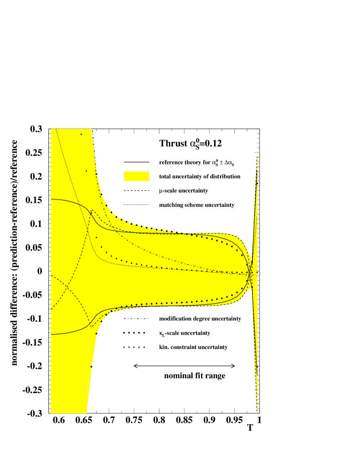
Figure 4: Theoretical uncertainties for thrust. The grey area represents the total theoretical uncertainty for the distribution. The first curve indicates the reference theory with maximum resp. minimum $\alpha_{s}$, which determines the theoretical uncertainty $\Delta\alpha_{s}$ for a given measurement $\alpha_{s}^{0}$. The other lines illustrate the different contributions to the theoretical uncertainty.

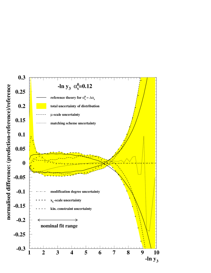
Figure 5: Theoretical uncertainties for $-\ln y_{3}$. The explanation is given in the caption of Fig. 4.

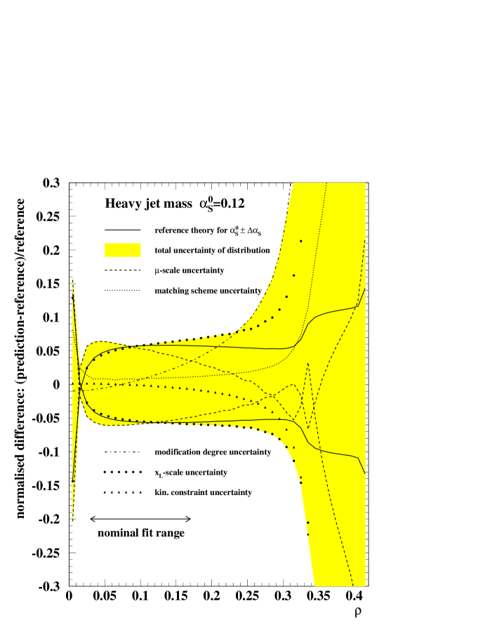
Figure 6: Theoretical uncertainties for heavy jet mass. The explanation is given in the caption of Fig. 4.

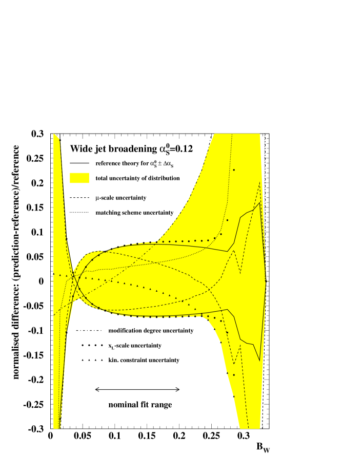
Figure 7: Theoretical uncertainties for wide jet broadening. The explanation is given in the caption of Fig. 4.

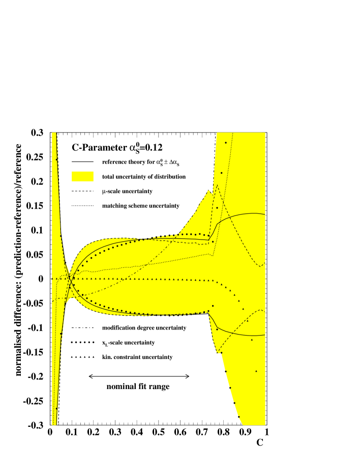
Figure 8: Theoretical uncertainties for $C$ parameter. The explanation is given in the caption of Fig. 4.

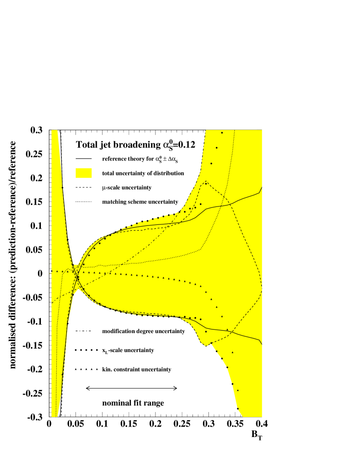
Figure 9: Theoretical uncertainties for total jet broadening. The explanation is given in the caption of Fig. 4.

As can be seen in Figs. 4–9, the total theoretical uncertainty, i.e. the uncertainty band, varies drastically across the distributions. The uncertainties are large, of the order of 30$\%$, at both ends of the spectra and reach a minimum of a few percent in the peak region. In the range of experimental fits for $\alpha_{s}$ the uncertainty of the distribution is between 5$\%$ and 10$\%$. This turns into an uncertainty for $\alpha_{s}$ between 3$\%$ and 6$\%$. There is also a considerable spread among the observables, the uncertainties for the total jet broadening are in the central part twice as large as for $-\ln y_{3}$.

A closer look at the individual components of the theoretical error reveals two major contributions: the variation of the renormalisation scale and of the $x_{L}$-scale. In the semi-inclusive region the $x_{\mu}$ variation generates the dominant uncertainty while in the three-jet region it is the variation of $x_{L}$. These two effects are clearly complementary. Going down in size of the uncertainty, the degree of modification as probed by the difference between $p=1$ and $p=2$ is important in the hard three-jet region, where this effect dominates. Both the kinematic constraint and the matching scheme uncertainty are rather small in the central part of the spectra and become somewhat larger at the multi-jet end.

The uncertainty of $\alpha_{s}$ is derived from the range of values leading to ‘valid’ predictions inside the uncertainty band. The resulting uncertainty depends on the fit range, which usually encloses the central part of the spectrum. The extreme, but still valid reference predictions, shown as full lines in Figs. 4–9, are in general determined in the central region, they touch the envelope of the uncertainty band at one point and remain inside the uncertainty band even outside the fit range.

5 Results

With the uncertainty band method as tool, all aspects of the theoretical systematic uncertainties for $\alpha_{s}$ can be studied in detail independent of a measured distribution. In Table 7 results for the total uncertainty as well as for individual components are given for a representative fit range and $\alpha_{s}=0.12$ as input.

	$T$	$-\ln y_{3}$	$\rho$	$B_{W}$	$C$	$B_{T}$
fit range	0.78-0.95	1.8-4.2	0.05-0.17	0.06-0.20	0.18-0.62	0.07-0.22
total	$+0.0057$	$+0.0028$	$+0.0044$	$+0.0055$	$+0.0058$	$+0.0068$
uncertainty	$-0.0055$	$-0.0030$	$-0.0045$	$-0.0054$	$-0.0054$	$-0.0062$
$x_{\mu}$	$+0.0055$	$+0.0027$	$+0.0028$	$+0.0018$	$+0.0052$	$+0.0062$
uncertainty	$-0.0055$	$-0.0008$	$-0.0039$	$-0.0033$	$-0.0053$	$-0.0059$
$x_{L}$	$+0.0048$	$+0.0017$	$+0.0041$	$+0.0053$	$+0.0044$	$+0.0045$
uncertainty	$-0.0047$	$-0.0029$	$-0.0042$	$-0.0053$	$-0.0046$	$-0.0059$
mod. degree	$-0.0001$	$+0.0002$	$-0.0001$	$-0.0004$	$-0.0003$	$+0.0003$
uncertainty
matching scheme	$+0.0004$	$-0.0007$	$+0.0005$	$+0.0018$	$+0.0014$	$+0.0014$
uncertainty
kinematic constraint	$0.0001$	$-0.0001$	$-0.0001$	$-0.0001$	$+0.0001$	$+0.0001$
uncertainty
total uncertainty	$+0.0062$	$+0.0028$	$+0.0052$	$+0.0066$	$+0.0065$	$+0.0077$
with $|\ln x_{L}|<0.6$	$-0.0059$	$-0.0032$	$-0.0052$	$-0.0066$	$-0.0061$	$-0.0073$
total uncertainty	$+0.0062$	$+0.0032$	$+0.0052$	$+0.0061$	$+0.0066$	$+0.0074$
with ‘fit’ method	$-0.0058$	$-0.0041$	$-0.0052$	$-0.0057$	$-0.0059$	$-0.0064$

Table 7: Theoretical uncertainties for $\alpha_{s}=0.12$ and fit ranges given in the first row. For each variable, the total theoretical uncertainty as well as uncertainties stemming from individual sources are given. In the last two rows concern results with more conservative theory assumptions.

The total uncertainty range from 3$\%$ for $-\ln y_{3}$ to 6$\%$ for the total jet broadening, with an overall average of 5$\%$. The uncertainties related to $x_{\mu}$ and $x_{L}$ are two-sided and in general asymmetric, the other uncertainties go in a single direction. The fact that the total uncertainty is larger than any of the individual ones is a consequence of the complementary collection of uncertainties of the distributions in the uncertainty band. A clear ranking in size of the different components of the theoretical uncertainty appears for all variables: variations of $x_{\mu}$ and $x_{L}$ are most important, followed by the matching scheme uncertainty, while the kinematic constraint and modification degree uncertainties are small and of similar size. Also given in Table 7 are uncertainty estimates obtained with more conservative assumptions, namely a larger range for $x_{L}$ ($|\ln x_{L}|<0.6$) and a fit of the reference prediction to the uncertainty band envelope (‘fit’ method).

Since the uncertainty is calculated with a fixed value of $\alpha_{s}$, the dependence of the result on the input value must be investigated. The input value, normally taken from an experimental measurement, depends on the observable and the centre-of-mass energy. For a theory defined up to ${\cal O}(\alpha_{s}^{2})$, the uncertainty is formally expected to be at ${\cal O}(\alpha_{s}^{3})$. The matching of fixed order and resummed calculations, however, may alter the scaling with $\alpha_{s}^{3}$. The evolution of the uncertainty with $\alpha_{s}$ is shown in Fig. 10. In this case the symmetric uncertainty is analysed, i.e. the mean of the upward and downward uncertainty.

Figure 10: Evolution of the theoretical uncertainty with $\alpha_{s}$. The lines are the result of a parameterisation scaling with $\alpha_{s}^{3}$.

A fit of the form $a+b\alpha_{s}^{3}$ gives a good description of the dependence of the uncertainty on $\alpha_{s}$. The parameters $a$ and $b$ obtained with the fit are given in Table 8 for each observable. In general $a$ is found to be substantially smaller than $b\alpha_{s}^{3}$, confirming that to a reasonable approximation the simple $\alpha_{s}^{3}$ scaling discussed above is observed.

Observable	$a$	$b$
$T$	$3.6\,10^{-4}$	$2.99$
$-\ln y_{3}$	$2.4\,10^{-4}$	$1.51$
$\rho$	$2.7\,10^{-4}$	$2.38$
$B_{W}$	$6.8\,10^{-4}$	$2.71$
$C$	$5.8\,10^{-4}$	$2.88$
$B_{T}$	$9.7\,10^{-4}$	$3.18$

Table 8: Parameterisation of the uncertainty evolution with $\alpha_{s}$ according to a form $a+b\alpha_{s}^{3}$.

The two main components of the theoretical uncertainty originate from the variations of $x_{\mu}$ and $x_{L}$. The size of the uncertainties depends crucially on the range of variation, nominally from $\frac{1}{2}$ to 2 for $x_{\mu}$ and from $\frac{2}{3}$ to $\frac{3}{2}$ for $x_{L}$. The dependence on the range choice is studied by re-scaling the variation range by a factor of $x_{R}$. Hence, the re-scaled range has an upper limit of $x_{up}*x_{R}$ ($x_{up}=2$ resp. $\frac{3}{2}$ for $x_{\mu}$ resp. $x_{L}$) and a lower limit of $x_{down}/x_{R}$ ($x_{down}=\frac{1}{2}$ resp. $\frac{2}{3}$ for $x_{\mu}$ resp. $x_{L}$). The effect of a range variation is expected to be linear in the logarithm of the re-scaling factor $x_{R}$ and the results are given as function of $\ln x_{R}$ for both the upper bound (positive error) and lower bound (negative error).

Figure 11: The dependence of the positive and negative uncertainty related to the variation of the renormalisation scale $x_{\mu}$. The width of the variation range is modified such that the lower endpoint is rescaled by $1/x_{R}$ and the upper limit by $x_{R}$.

Figure 12: The dependence of the positive and negative uncertainty related to the variation of the logarithmic re-scaling factor $x_{L}$. The width of the variation range is modified such that the lower endpoint is rescaled by $1/x_{R}$ and the upper limit by $x_{R}$.

The dependence of the $x_{\mu}$ component of the uncertainty on the range of variation is shown in Fig. 11. The size of uncertainty increases rapidly with the width of the range, the positive error flattens at large ranges for $-\ln y_{3}$, $\rho$ and $B_{W}$. The shape of the dependence is similar for all variables. The case of the $x_{L}$ component is shown in Fig. 12. Here the rise at small variation ranges is even steeper than for $x_{\mu}$. For the variable $-\ln y_{3}$ the evolution is significantly flatter than for all other variables, a similar effect would have been observed with a quadratic re-scaling of the variation range.

Finally, the dependence of the uncertainty on the fit range experimentally used to extract $\alpha_{s}$ from the distribution is studied. For this purpose the uncertainty band method including all uncertainty sources is applied to each bin of the distribution, as shown in Fig. 13. In the central part of the distribution the uncertainty is reasonably constant and stable with respect to variations of one or two bins at each end. Approaching the peak of the distributions or the extreme three-jet region, however, induces rapidly growing uncertainties. This dependence should be kept in mind when selecting a fit range.

Figure 13: The dependence of the positive and negative uncertainty on the value of the observable. All components of the uncertainty are included.

The theory uncertainty studies described here are all carried out on purely perturbative predictions. One could instead envisage carrying out these studies after correction to hadron-level. Whether this actually makes a difference or not depends on the details of how the hadronisation is included, for example whether as a bin-by-bin multiplicative factor, a simple shift of the distribution, or a transfer matrix. However, since hadronisation corrections will have similar effects both on the various alternate theory curves and on the reference prediction, the net impact of hadronisation is expected to be rather small and hence it is simplest and most transparent to carry out the analysis at a purely perturbative level

6 Conclusion

In this paper, a new method is presented for the assessment of theoretical uncertainties in $\alpha_{s}$. This method evaluates the systematic uncertainty of the parameter $\alpha_{s}$ from the uncertainty of the prediction for the distributions from which it is extracted. After a comprehensive review of theoretical predictions for measurements of $\alpha_{s}$ from event-shape distributions in ${\rm e}^{+}{\rm e}^{-}$ annihilation, the uncertainties of such predictions are estimated with an uncertainty band method which incorporates several variations of the theory differing in subleading terms and includes a new test for re-scaling the resummed logarithmic variables. As the uncertainty band method can compute these perturbative uncertainties of $\alpha_{s}$ independently of a measured event-shape distribution, it is especially suited for an unbiased combination of several observables or experiments.

The recommended method for computing the central result is to use the modified Log(R) matching scheme with $x_{\mu}=x_{L}=1$, $p=1$ and values for $y_{\rm max}$ given in Table 2. The assessment of the perturbative uncertainty consists of a variation of the renormalisation scale $x_{\mu}$ from 0.5 to 2, of the logarithmic re-scaling factor $x_{L}$ from $\frac{2}{3}$ to $\frac{3}{2}$, of a replacement of the modified Log(R) matching scheme by the modified R matching scheme, of the degree of modification $p=1$ by $p=2$ and of the kinematic constraint $y_{\rm max}$ by its alternative $y^{\prime}_{\rm max}$ given in Table 2. The different uncertainties should be combined with the uncertainty band method. Proposals are made for more conservative uncertainty estimates; these are a larger range for the re-scaling factor $|\ln x_{L}|<0.6$ and an alternative operating mode of the uncertainty band method.

To combine several measurements from different observables or experiments the perturbative uncertainties of the individual measurements should be re-estimated with the above method using a common input value for $\alpha_{s}(M_{\rm Z})$ in the uncertainty band method. This input value should of course be consistent with the final result obtained iteratively.

Following these instructions even existing measurements of $\alpha_{s}$ can be equipped with an up-to-date estimation of their perturbative uncertainty and then used in a consistent combination.

References

- [1] R.K. Ellis, D.A. Ross and A.E. Terrano, Nucl. Phys. B 178 (1981) 421
-
[2]
Yu.L. Dokshitzer and B.R. Webber,
Phys. Lett. B 352 (1995) 451;
Phys. Lett. B 404 (1997) 321;
Yu.L. Dokshitzer et al., J. High Energy Phys. 05 (1998) 003. -
[3]
J. Abreu et al., DELPHI collaboration, Phys. Lett. B 456 (1999) 322;
M. Acciarri et al., L3 collaboration Phys. Lett. B 489 (2000) 65;
P.A. Movilla et al., Eur. Phys. J. C 22 (2001) 1;
J. Abdallah et al., DELPHI collaboration, Eur. Phys. J. C 29 (2003) 285. - [4] P.A. Movilla Fernández, hep-ex/0209022, MPI-PH-2002-12
- [5] LEPQCD working group, note in preparation
-
[6]
K.G. Chetyrkin et al., Phys. Rept. 277 (1996) 189;
E. Tournefier, LAL 98-67 - [7] LEPEW working group and LEP collaborations, CERN-EP-2002-091, hep-ex/0212036
- [8] K.G. Chetyrkin et al., Phys. Rev. Lett. 79 (1997) 2184.
- [9] S. Chekanov et al., ZEUS Collaboration, Phys. Rev. D 67 (2003) 012007.
-
[10]
S. Catani et al., Phys. Lett. B 263 (1991) 491;
Phys. Lett. B 272 (1991) 368. - [11] S. Catani, L. Trentadue, G. Turnock and B. R. Webber, Nucl. Phys. B 407 (1993) 3
- [12] G. Dissertori and M. Schmelling, Phys. Lett. B 361 (1995) 167.
-
[13]
S. Catani et al., Phys. Lett. B 295 (1992) 269;
Yu.L. Dokshitzer et al., J. High Energy Phys. 01 (1998) 11. - [14] S. Catani et al., Phys. Lett. B 427 (1998) 377.
- [15] A. Banfi et al., J. High Energy Phys. 201 (2002) 18.
- [16] M. Dasgupta and G. P. Salam, Eur. Phys. J. C 24 (2002) 213; M. Dasgupta and G. P. Salam, J. High Energy Phys. 0208 (2002) 032.
-
[17]
S. Brandt et al., Phys. Lett. 12 (1964) 57;
E. Farhi, Phys. Rev. Lett. 39 (1977) 1587. -
[18]
T. Chandramohan and L. Clavelli, Nucl. Phys. B 184 (1981) 365;
L. Clavelli and D. Wyler, Phys. Lett. B 103 (1981) 383. - [19] P.E.L. Rakow and B.R. Webber, Nucl. Phys. B 191 (1981) 63.
-
[20]
G. Parisi, Phys. Lett. B 74 (1978) 65;
J.F. Donoghue et al., Phys. Rev. D 20 (1979) 2759. -
[21]
S. Catani et al., Phys. Lett. B 269 (1991) 432;
W.J. Stirling et al., Proceedings of the Durham Workshop, J. Phys. G 17 (1991) 1567;
N. Brown and W.J. Stirling, Phys. Lett. B 252 (1990) 657;
S. Bethke et al., Nucl. Phys. B 370 (1992) 310. - [22] S. Catani and M. Seymour, Nucl. Phys. B 485 (1997) 291.
-
[23]
E. Gardi and J. Rathsman, Nucl. Phys. B 609 (2001) 123;
E. Gardi and J. Rathsman, Nucl. Phys. B 638 (2002) 243;
E. Gardi and L. Magnea, J. High Energy Phys. 0308 (2003) 30. - [24] T. Sjöstrand et al., PYTHIA, Comput. Phys. Commun. 135 (2001) 238.
- [25] G. Rodrigo, A. Santamaria and M. S. Bilenky, Phys. Rev. Lett. 79 (1997) 193; P. Nason and C. Oleari, Nucl. Phys. B 521 (1998) 237; A. Brandenburg and P. Uwer, Nucl. Phys. B 515 (1998) 279.
- [26] The ALEPH collaboration, Eur. Phys. J. C 18 (2000) 1.
- [27] F. Krauss and G. Rodrigo, Phys. Lett. B 576 (2003) 135.
-
[28]
L. W. Garland, T. Gehrmann, E. W. N. Glover, A. Koukoutsakis and E. Remiddi,
Nucl. Phys. B 642 (2002) 227;
S. Moch, P. Uwer and S. Weinzierl, Acta Phys. Pol., Ser. B: 33 (2002) 2921. -
[29]
S. Weinzierl,
J. High Energy Phys. 03 (2003) 062;
J. High Energy Phys. 07 (2003) 052.
- [30] E. W. N. Glover, Nucl. Phys. Proc. Suppl. 116 (2003) 3.
- [31] G. Bozzi, S. Catani, D. de Florian and M. Grazzini, Phys. Lett. B 564 (2003) 65.