Generalized Parton Distributions at $x\rightarrow 1$

Abstract

Generalized parton distributions at large $x$ are studied in perturbative QCD approach. As $x\rightarrow 1$ and at finite $t$, there is no $t$ dependence for the GPDs which means that the active quark is at the center of the transverse space. We also obtain the power behavior: $H_{q}^{\pi}(x,\xi,t)\sim(1-x)^{2}/(1-\xi^{2})$ for pion; $H_{q}(x,\xi,t)\sim(1-x)^{3}/(1-\xi^{2})^{2}$ and $E_{q}(x,\xi,t)\sim(1-x)^{5}/(1-\xi^{2})^{3}f(\xi)$ for nucleon, where $f(\xi)$ represents the additional dependence on $\xi$.

In recent years, there has been considerable interest in generalized parton distributions (GPDs) Ji:1996ek ; Muller:1998fv ; Radyushkin:1997ki , which were introduced originally to understand the quark and gluon contributions to the proton spin Ji:1996ek . They are also related to the quantum phase space distributions of partons in the hadrons wigner . The theoretical framework of the GPDs and their implications about the deeply virtual Compton scattering, deeply virtual meson production, and the doubly-virtual Compton scattering have been well established Ji:1998pc ; Radyushkin:2000uy ; Goeke:2001tz ; Belitsky:2001ns ; Diehl:2003ny ; Guidal:2002kt ; Belitsky:2002tf . Apart from the renormalization scale, the GPDs depend on the momentum transfer $t$, the light-cone momentum fraction $x$, and the skewness parameter $\xi$ which measures the momentum transfer along the light-cone direction. In phenomenology, the GPDs are parameterized through the double-distributions Radyushkin:1998bz and fit to the experimental data Goeke:2001tz ; Belitsky:2001ns ; Diehl:2003ny ; Guidal:2002kt ; Belitsky:2002tf . However, these parameterizations have too much freedom, and we still have a long way to go for a complete understanding of the GPDs. In this context, any theoretical result on the behavior of GPDs will provide important information. For example, the polynomality condition Ji:1998pc , and the positivity constraints Pobylitsa:2001nt have already played significant roles in the parametrizations of GPDs. The light-cone framework provides useful guidelines for calculating the GPDs once the wave functions are known Brodsky:2000xy . More recently, the GPDs at large $t$ have been explored Hoodbhoy:2003uu , yielding important constraints as well.

In this paper, we study the GPDs in the kinematic limit of $x\rightarrow 1$. For the forward parton distribution, a power behavior at large $x$ was predicted based on the power counting rules, for example, $(1-x)^{2}$ for pion, and $(1-x)^{3}$ for nucleon Drell:1969km ; West:1970av ; Brodsky:1973kr ; Matveev:ra ; Farrar:yb ; Brodsky:1994kg . This power behavior comes from the fact that the hard gluon exchanges dominate the structure functions at $x\rightarrow 1$, and is calculable in perturbative QCD Lepage:1980fj ; Mueller:sg . In this paper, we will follow these ideas to analyze the dependence of GPDs on the three variables $x$, $\xi$ and $t$ in the limit of $x\rightarrow 1$. We use the QCD factorization approach, and express the GPDs in terms of the distribution amplitudes of hadrons. In the limit of $x\rightarrow 1$, the power behavior of the GPDs does not depend on a particular input of the distribution amplitudes, and therefore can be predicted model-independently. More importantly, the $\xi$ and $t$ dependences can also be calculated. For example, we find that there is no $t$-dependence at $x\rightarrow 1$, which agrees with the previous intuitions Burkardt:2003ck .

We take $(1-x)$ as a small parameter, and expand the GPDs in terms of $(1-x)$. In the process, we assume the variables $\xi$ and $t$ finite. Finite $\xi$ means $\xi<x$ and restricts our analysis valid in the DGLAP region for the GPDs. The relevant Feynman diagrams are shown in Fig. 1 for pion, and in Fig. 2 for nucleon for a typical contribution. The variables $P$ and $P^{\prime}$ are the initial and final state hadron momenta, respectively, and $t=\Delta^{2}=(P-P^{\prime})^{2}$. We further introduce two vectors $\overline{P}$ and $n$: $\overline{P}=(P+P^{\prime})/2$, $n^{2}=0$, and $n\cdot\overline{P}=1$. The skewness parameter is defined as $\xi=-n\cdot(P^{\prime}-P)/2$. The initial and final light-cone momenta of the quarks are then $(x+\xi)$ and $(x-\xi)$, respectively. In the following, we will neglect the masses of the hadrons, and then $t=-\vec{\Delta}_{\perp}^{2}/(1-\xi^{2})$ where $\vec{\Delta}_{\perp}$ is the transverse part of the momentum transfer $\Delta$.

As shown in Fig. 1, the intermediate state has momentum $k$ which will be integrated out. To avoid an infrared divergence, we keep $k_{\perp}$ much larger than $\Lambda_{\rm QCD}$. The offshellness of the quark and gluon propagators are on the order of $\vec{k}_{\perp}^{2}/(1-x)$. So, we have the following hierarchy of scales in the limit of $x\rightarrow 1$: $\vec{k}_{\perp}^{2}/(1-x)\gg\vec{k}_{\perp}^{2}\gg\Lambda_{\rm QCD}^{2}$, and $\vec{k}_{\perp}^{2}/(1-x)\gg(-t)$ as well. These relations will be used to get the leading-order results, and any higher power in $(1-x)$ will be neglected.

The GPD $H(x,\xi,t)$ for pion is defined as

$$H_{q}(x,\xi,t) \!\!=\!\!\frac{1}{2}\int\frac{d\lambda}{2\pi}e^{i\lambda x}\left\langle\pi;P^{\prime}\left|\overline{\psi}_{q}\left(-\frac{\lambda}{2}n\right)\!\!\not\!n{\cal L}\psi_{q}\left(\frac{\lambda}{2}n\right)\right|\pi;P\right\rangle\ ,$$

where ${\cal L}$ represents the light-cone gauge link. We work in Feynman gauge, and the leading-order diagrams were shown in Fig. 1, where the double lines represent the eikonal contributions from the gauge link, and the cross indicates the intermediate state on mass shell. The initial and final states are replaced by the light-cone Fock component of hadrons with the minimal number of partons. After integrating over the internal transverse momentum $l_{\perp}$, the light-cone wave function leads to the distribution amplitude, $\phi(x)=\int\frac{d^{2}l_{\perp}}{(2\pi)^{3}}\psi(x,l_{\perp})$.

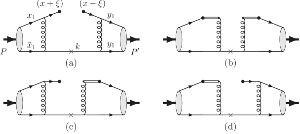
Figure 1: Leading order contributions to the generalized parton distribution $H_{q}(x,\xi,t)$ for pion at large $x$. The crosses represent the intermediated states, and the double lines for the eikonal term from the gauge link.

The calculation of the diagrams in Fig. 1 is straightforward, and the result is

$$H_{q}^{\pi}(x,\xi,t) = \int\frac{d^{2}k_{\perp}}{(2\pi)^{3}}\frac{1}{(2k\cdot P)(2k\cdot P^{\prime})}{\cal I}(x,\xi)\ .$$ (1)

The integral ${\cal I}$ depends on the distribution amplitudes of the initial and final states,

$${\cal I}(x,\xi) = (4\pi\alpha_{s}C_{F})^{2}\int dx_{1}dy_{1}\frac{\phi(x_{1})\phi^{*}(y_{1})}{\overline{x}_{1}\overline{y}_{1}}\left(1+\frac{1}{\overline{x}_{1}-\frac{1-x}{1+\xi}}\right)\left(1+\frac{1}{\overline{y}_{1}-\frac{1-x}{1-\xi}}\right)\ ,$$

where $C_{F}=4/3$ and $\overline{x}_{1}=1-x_{1}$. The integral becomes a constant in the limit of $x\rightarrow 1$. In Eq. (1), the denominator factors $2(k\cdot P)$ and $2(k\cdot P^{\prime})$ in come from the gluon propagators in the diagrams. They depend on the momentum transfer $t$ in general. However, if expanded at small $(1-x)$, they become

$$\frac{1}{2k\cdot P} = \frac{1-x}{\vec{k}_{\perp}^{2}(1+\xi)}\left[1+\frac{(1-x)^{2}(1-\xi^{2})t}{4(1+\xi)^{2}\vec{k}_{\perp}^{2}}\right]\ ,$$

$$\frac{1}{2k\cdot P^{\prime}} = \frac{1-x}{\vec{k}_{\perp}^{2}(1-\xi)}\left[1+\frac{(1-x)^{2}(1-\xi^{2})t}{4(1-\xi)^{2}\vec{k}_{\perp}^{2}}\right]\ ,$$ (2)

which implys that there is no $t$-dependence in the leading order, and any dependence will be suppressed by a factor of $(1-x)^{2}$. Since the propagators are the only source of the $t$-dependence of the GPD in Eq. (1), we conclude that at $x\rightarrow 1$ the GPD $H(x,\xi,t)$ for pion has no $t$-dependence, and any $t$-dependence must be suppressed by a factor of $(1-x)^{2}$. These conclusions agree with the analysis in the impact parameter dependent picture of the GPDs at $\xi=0$ Burkardt:2003ck , while our results are valid for any finite value of $\xi$.

Collecting the above results, we have the GPD $H(x,\xi,t)$ for the pion in the limit of $x\rightarrow 1$,

$$H_{q}^{\pi}(x,\xi,t)=\frac{(1-x)^{2}}{1-\xi^{2}}\int\frac{d^{2}k_{\perp}}{(2\pi)^{3}}\frac{1}{(k_{\perp}^{2}+\Lambda^{2})^{2}}{\cal I}\ .$$ (3)

There is an infrared divergence where the transverse momentum $k_{\perp}$ becomes soft. This divergence breaks the factorization in principle. However, this does not change the power behavior. Nevertheless, we include a regulator $\Lambda$ to regulate such divergence Mueller:sg . Like the forward parton distributions, a power behavior is found here for the GPDs in Eq. (3). If we take $\xi=0$ and $t=0$, Eq. (3) will reproduce the forward parton distribution of pion. So, in the limit of $x\rightarrow 1$, the GPD $H(x,\xi,t)$ for pion can be related to the forward parton distribution $q^{\pi}(x)$,

$$H_{q}^{\pi}(x,\xi,t)=\frac{1}{1-\xi^{2}}q^{\pi}(x)\ .$$ (4)

We note that the above equality saturates the positivity constraints Pobylitsa:2001nt ; Diehl:2003ny if we take the power behavior for valence quark distribution $q^{\pi}(x)\sim(1-x)^{2}$.

We turn now to the study of GPDs for the nucleon. Since the leading Fock component of nucleon has three partons, many more diagrams will contribute. Here we only show a particular diagram in Fig. 2. There are two intermediate momenta, $k_{1}$ and $k_{2}$. Similar to the above analysis for the pion case, we have a hierarchy of scales: $\langle\vec{k}_{\perp}^{2}\rangle/(1-x)\gg\langle\vec{k}_{\perp}^{2}\rangle\gg\Lambda^{2}_{\rm QCD}$ and $\langle\vec{k}_{\perp}^{2}\rangle/(1-x)\gg(-t)$, where $\langle\vec{k}_{\perp}^{2}\rangle$ represents the typical transverse momentum scale, $\langle\vec{k}_{\perp}^{2}\rangle\sim\langle\vec{k}_{1\perp}^{2}\rangle\sim\langle\vec{k}_{1\perp}^{2}\rangle$. Again, we are only interested in the leading-order result, and neglect any higher-order corrections in $(1-x)$.

The calculations are performed in the helicity bases for the initial and final nucleon states $(\lambda^{\prime},\lambda)$, in which the following off-forward matrix elements are defined:

$${\cal H}_{\lambda^{\prime}\lambda} = \!\!\frac{1}{2\sqrt{1-\xi^{2}}}\int\frac{d\lambda}{2\pi}e^{i\lambda x}\left\langle P^{\prime},\lambda^{\prime}\left|\overline{\psi}_{q}\left(-\frac{\lambda}{2}n\right)\!\!\not\!n{\cal L}\psi_{q}\left(\frac{\lambda}{2}n\right)\right|P,\lambda\right\rangle\ .$$

The helicity non-flip amplitude has contributions from both $H$ and $E$ GPDs, while the helicity flip one only has the contribution from $E$ GPDDiehl:2003ny ,

$${\cal H}_{\uparrow\uparrow} = {\cal H}_{\downarrow\downarrow}=H_{q}(x,\xi,t)-\frac{\xi^{2}}{1-\xi^{2}}E_{q}(x,\xi,t)\ ,$$

$${\cal H}_{\downarrow\uparrow} = -{\cal H}_{\uparrow\downarrow}^{*}=\frac{\Delta^{x}+i\Delta^{y}}{2M_{p}(1-\xi^{2})}E_{q}(x,\xi,t)\ .$$ (5)

We will show how the diagram in Fig. 2 contribute to these amplitudes.

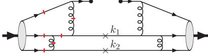
Figure 2: The typical diagram contributing to the nucleon GPDs at $x\rightarrow 1$. The quark helicity configuration is $\{\uparrow\downarrow\uparrow\}$. The bars indicate the places where we need to consider the internal transverse momentum expansion to get helicity flip amplitude.

The helicity non-flip amplitude for the diagram of Fig. 2 has the following form,

$${\cal H}_{\uparrow\uparrow}=\int\frac{d^{2}k_{1\perp}d^{2}k_{2\perp}}{(2\pi)^{3}}\int\frac{d\alpha}{\alpha\beta(1-x)}\left(\frac{1}{2P\cdot(k_{1}+k_{2})}\frac{1}{2P^{\prime}\cdot(k_{1}+k_{2})}\right)^{2}\frac{P^{\prime}\cdot k_{1}}{P^{\prime}\cdot k_{2}}{\cal I}_{p}(x,\xi)\ ,$$ (6)

where any other factors (such as color factors and coupling constants, etc.) are included in the integral ${\cal I}_{p}(x,\xi)$. This integral depends on the leading-twist distribution amplitudes of the proton Braun:2000kw , and will become a constant integral at the limit of $x\rightarrow 1$. The longitudinal momentum fractions of $k_{1}$ and $k_{2}$ are defined as $n\cdot k_{1}=\alpha(1-x)$, $n\cdot k_{2}=\beta(1-x)$, and $\alpha+\beta=1$. For the propagators, we make expansions at small $(1-x)$ as before, for example,

$$\frac{1}{2P\cdot(k_{1}+k_{2})}=\frac{\langle\vec{k}_{\perp}^{2}\rangle}{1-x}(1+\xi)\left[1+{\cal O}((1-x)^{2})\frac{t}{\langle\vec{k}_{\perp}^{2}\rangle}+\cdots\right]\ ,$$ (7)

which again has no $t$-dependence at the leading order, and any $t$ dependence is suppressed by a factor of $(1-x)^{2}$. All propagators in Eq. (6) have this property, and all other diagrams which contribute to ${\cal H}_{\uparrow\uparrow}$ at the leading order have the same dependence on $t$. The $t$ dependence of nucleon GPDs is the same as that of the pion: there is no $t$ dependence and any dependence is suppressed by a factor of $(1-x)^{2}$. In addition, every diagram contributes the same dependence on $\xi$. Adding all of the contributions together, we get

$${\cal H}_{\uparrow\uparrow}=\frac{(1-x)^{3}}{(1-\xi^{2})^{2}}\int\frac{d^{2}k_{1\perp}d^{2}k_{2\perp}}{(2\pi)^{3}}\int\frac{d\alpha}{\alpha\beta}F(\alpha,k_{1\perp},k_{2\perp},\Lambda){\cal I}_{p}\ ,$$ (8)

where the function $F$ is of order $1$ at $x\rightarrow 1$. Here we also include a regulator $\Lambda$ in $F$ to regulate the infrared divergences in the $k_{1\perp}$ and $k_{2\perp}$ integrations. If we take $\xi=0$ and $t=0$, the above results will reproduce the forward parton distribution at large $x$. That means we can have,

$${\cal H}_{\uparrow\uparrow}=\frac{1}{(1-\xi^{2})^{2}}q(x)\sim\frac{(1-x)^{3}}{(1-\xi^{2})^{2}}\ ,$$ (9)

at $x\rightarrow 1$.

Since hard scattering conserves the quark helicity, in order to get the helicity flip amplitude ${\cal H}_{\uparrow\downarrow}$ we must include non-zero orbital angular momentum either for the initial or final states. In other words, we need to consider the light-cone Fock components of hadrons with at least one unit of orbital angular momentum Ji:2002xn . The calculation for the helicity flip amplitudes are much more complicated than that for the helicity conserving ones. The method we are using follows Ref. Belitsky:2002kj where the helicity flip Pauli form factor was calculated in perturbative QCD. We will sketch the method and summarize the main results, but skip the detailed derivations.

First, we keep the internal transverse momenta $l_{\perp}$ of the scattering partons in the hard partonic scattering amplitudes. Then, we expand the amplitudes at small $l_{\perp}$. Since $\Delta_{\perp}$ is the only relevant external transverse momentum, the expansion of the amplitudes will be proportional to $\vec{\Delta}_{\perp}\cdot\vec{l}_{\perp}$ or $\vec{\Delta}_{\perp}\times\vec{l}_{\perp}$. Integrating these terms over $l_{\perp}$ with the light-cone wave functions, we will get, e.g., $\int d^{2}l_{\perp}\vec{\Delta}_{\perp}\cdot\vec{l}_{\perp}(l_{\perp}^{x}+il_{\perp}^{y})\psi^{(3,4)}\sim(\Delta_{\perp}^{x}+i\Delta_{\perp}^{y})\Phi^{(3,4)}$, and $\int d^{2}l_{\perp}\vec{\Delta}_{\perp}\times\vec{l}_{\perp}(l_{\perp}^{x}+il_{\perp}^{y})\psi^{(3,4)}\sim-i(\Delta_{\perp}^{x}+i\Delta_{\perp}^{y})\Phi^{(3,4)}$, where $\psi^{(3,4)}$ are the light-cone wave functions for the Fock state with one unit orbital angular momentum Ji:2002xn , and $\Phi^{(3,4)}$ are the related twist-four distribution amplitudes Braun:2000kw . Thus, the final results of ${\cal H}_{\uparrow\downarrow}$ depend on the twist-three and twist-four distribution amplitudes of the nucleon.

We must consider the expansions for all propagators and quark wave functions which have dependence on $l_{\perp}$. As an example, in Fig. 2 we indicate all places where the $l_{\perp}$ expansion should be considered if the initial state has one unit of orbital angular momentum. These expansions will give additional power of $(1-x)^{2}$, leading to the helicity flip amplitudes suppressed by $(1-x)^{2}$. For instance, one of the gluon propagators in the diagram of Fig. 2 has the following expansion,

$$\frac{1}{(k_{2}-x_{3}P-l_{\perp})^{2}}=\frac{1}{(k_{2}-x_{3}P)^{2}}\left[1-\frac{\beta(1-x)^{2}\vec{\Delta}_{\perp}\cdot\vec{l}_{\perp}}{(1+\xi)^{2}\vec{k}_{2\perp}^{2}}\right]\ .$$ (10)

Extracting the expansion coefficients, and combing with other factors in the amplitude, we get the contribution to the helicity flip amplitude ${\cal H}_{\downarrow\uparrow}$ from this term: ${\cal H}_{\downarrow\uparrow}\sim(1-x)^{5}/(1-\xi^{2})^{2}(1+\xi)^{2}$. Adding the similar contribution from the final state expansion, we get ${\cal H}_{\downarrow\uparrow}\sim(1-x)^{5}/(1-\xi^{2})^{2}(1/(1+\xi)^{2}+1/(1-\xi)^{2})=(1-x)^{5}(1+\xi^{2})/(1-\xi^{2})^{4}$. All expansions result in the same suppression of $(1-x)^{2}$. However, they do not contribute the same dependence on $\xi$. For example, the quark wave function expansions lead to ${\cal H}_{\downarrow\uparrow}\sim(1-x)^{5}/(1-\xi^{2})^{4}$. In summary, the helicity flip amplitude will have the following result at $x\rightarrow 1$,

$${\cal H}_{\downarrow\uparrow}\sim(\Delta_{\perp}^{x}+i\Delta_{\perp}^{y})\frac{(1-x)^{5}}{(1-\xi^{2})^{4}}f(\xi)\ .$$ (11)

Here $f(\xi)$ represents an additional dependence on $\xi$, which will depend on the input of the twist-three and twist-four distribution amplitudes of the nucleon. From this, we deduce the behavior of GPD $E_{q}(x,\xi,t)$ as,

$$E_{q}(x,\xi,t)\sim\frac{(1-x)^{5}}{(1-\xi^{2})^{3}}f(\xi)\ .$$ (12)

Comparing with Eq. (9), we can neglect the $E_{q}$ contribution to the helicity non-flip amplitude, and then we have $H_{q}(x,\xi,t)\sim(1-x)^{3}/(1-\xi^{2})^{2}$. So, in the limit of $x\rightarrow 1$, $H_{q}(x,\xi,t)$ can be related to the forward quark distribution $q(x)$,

$$H_{q}(x,\xi,t)=\frac{1}{(1-\xi^{2})^{2}}q(x)\ .$$ (13)

Again this relation saturates the positivity constraint Diehl:2003ny ; Pobylitsa:2001nt for nucleon GPDs if the forward quark distribution takes the power behavior at large $x$: $q(x)\sim(1-x)^{3}$.

Before concluding, a few cautionary comments are in the order. First, we omit the scale dependence of the GPDs. The scale dependence at large $x$ is not just the simple DGLAP evolution Brodsky:1994kg ; Manohar:2003vb . In our calculations we implicitly assume $Q^{2}(1-x)\gg\Lambda_{\rm QCD}^{2}$. Second, at the limit of $x\rightarrow 1$ there exist $\alpha_{s}^{n}{\rm log}^{m}(1/(1-x))$ for $m\leq 2n$ series terms which need to be resummed, leading to a Sudakov form factor suppression Lepage:1980fj ; Mueller:sg ; Manohar:2003vb ; Sterman:1986aj . Third, the soft mechanism might contribute to the GPDs Radyushkin:1998rt at $x\rightarrow 1$. We did not include such effects in our analysis.

In summary, we have studied generalized parton distributions at $x\rightarrow 1$. We found that the pion’s GPD $H_{q}^{\pi}(x,\xi,t)\sim(1-x)^{2}/(1-\xi^{2})$, and the nucleon’s GPD $H_{q}(x,\xi,t)\sim(1-x)^{3}/(1-\xi^{2})^{2}$ and $E_{q}(x,\xi,t)\sim(1-x)^{5}/(1-\xi^{2})^{4}f(\xi)$. There is no $t$ dependence, and any dependence is suppressed by a factor of $(1-x)^{2}$. These results can provide important information on the GPDs’ parameterizations.

We thank Xiangdong Ji for pointing out the $t$ dependence of the GPDs at large $x$ and many other stimulating discussions. We also thank Andrei Belitsky, Stan Brodsky, and Jianwei Qiu for useful comments. This work was supported by the U. S. Department of Energy via grants DE-FG02-93ER-40762.

References

- (1) X. Ji, Phys. Rev. Lett. 78, 610 (1997); Phys. Rev. D 55, 7114 (1997).
- (2) D. Muller, D. Robaschik, B. Geyer, F. M. Dittes and J. Horejsi, Fortsch. Phys. 42, 101 (1994).
- (3) A. V. Radyushkin, Phys. Rev. D 56, 5524 (1997).
- (4) X. Ji, Phys. Rev. Lett. 91, 062001 (2003). A. V. Belitsky, X. Ji and F. Yuan, arXiv:hep-ph/0307383. M. Burkardt, Phys. Rev. D 62, 071503 (2000) [Erratum-ibid. D 66, 119903 (2002)].
- (5) X. Ji, J. Phys. G 24, 1181 (1998).
- (6) A. V. Radyushkin, arXiv:hep-ph/0101225.
- (7) K. Goeke, . V. Polyakov and M. Vanderhaeghen, Prog. Part. Nucl. Phys. 47, 401 (2001).
- (8) A. V. Belitsky, D. Muller and A. Kirchner, Nucl. Phys. B 629, 323 (2002) [arXiv:hep-ph/0112108].
- (9) M. Diehl, arXiv:hep-ph/0307382.
- (10) M. Guidal and M. Vanderhaeghen, Phys. Rev. Lett. 90, 012001 (2003)
- (11) A. V. Belitsky and D. Muller, Phys. Rev. Lett. 90, 022001 (2003); A. V. Belitsky and D. Muller, arXiv:hep-ph/0307369.
- (12) A. V. Radyushkin, Phys. Lett. B 449, 81 (1999).
- (13) P. V. Pobylitsa, Phys. Rev. D 65, 077504 (2002).
- (14) S. J. Brodsky, M. Diehl and D. S. Hwang, Nucl. Phys. B 596, 99 (2001); M. Diehl, T. Feldmann, R. Jakob and P. Kroll, Nucl. Phys. B 596, 33 (2001) [Erratum-ibid. B 605, 647 (2001)].
- (15) P. Hoodbhoy, X. Ji and F. Yuan, arXiv:hep-ph/0309085.
- (16) S. D. Drell and T. M. Yan, Phys. Rev. Lett. 24, 181 (1970).
- (17) G. B. West, Phys. Rev. Lett. 24, 1206 (1970).
- (18) S. J. Brodsky and G. R. Farrar, Phys. Rev. Lett. 31, 1153 (1973).
- (19) V. A. Matveev, R. M. Muradian and A. N. Tavkhelidze, Lett. Nuovo Cim. 7, 719 (1973).
- (20) G. R. Farrar and D. R. Jackson, Phys. Rev. Lett. 35, 1416 (1975).
- (21) S. J. Brodsky, M. Burkardt and I. Schmidt, Nucl. Phys. B 441, 197 (1995).
- (22) G. P. Lepage and S. J. Brodsky, Phys. Rev. D 22, 2157 (1980).
- (23) A. H. Mueller, Phys. Rept. 73, 237 (1981).
- (24) M. Burkardt, arXiv:hep-ph/0309116; Int. J. Mod. Phys. A 18, 173 (2003).
- (25) V. Braun, R. J. Fries, N. Mahnke and E. Stein, Nucl. Phys. B 589, 381 (2000) [Erratum-ibid. B 607, 433 (2001)].
- (26) X. Ji, J. P. Ma and F. Yuan, Nucl. Phys. B 652, 383 (2003); arXiv:hep-ph/0304107.
- (27) A. V. Belitsky, X. Ji and F. Yuan, Phys. Rev. Lett. 91, 092003 (2003) .
- (28) A. V. Manohar, arXiv:hep-ph/0309176; and references therein.
- (29) G. Sterman, Nucl. Phys. B 281, 310 (1987).
- (30) A. V. Radyushkin, Phys. Rev. D 58, 114008 (1998).