Signatures of supernova neutrino oscillations in the Earth mantle and core

Abstract

The Earth matter effects on supernova (SN) neutrinos can be identified at a single detector through peaks in the Fourier transform of their “inverse energy” spectrum. The positions of these peaks are independent of the SN models and therefore the peaks can be used as a robust signature of the Earth matter effects, which in turn can distinguish between different neutrino mixing scenarios. Whereas only one genuine peak is observable when the neutrinos traverse only the Earth mantle, traversing also the core gives rise to multiple peaks. We calculate the strengths and positions of these peaks analytically and explore their features at a large scintillation detector as well as at a megaton water Cherenkov detector through Monte Carlo simulations. We propose a simple algorithm to identify the peaks in the actual data and quantify the chances of a peak identification as a function of the location of the SN in the sky.

1 Introduction

The neutrino spectra that arrive at the Earth from a core collapse supernova (SN) have information about the neutrino masses and mixings encoded in them. The $\sim 20$ neutrinos observed from SN 1987A were extensively used trying to constrain the solar neutrino parameters as well as $\theta_{13}$ and the neutrino mass hierarchy [1, 2, 3, 4]. The determination of neutrino parameters depends crucially on our understanding of the primary neutrino fluxes produced inside the SN. In spite of large uncertainties on these primary fluxes, some of their robust features may be exploited to identify the type of neutrino mass hierarchy and put bounds on the mixing of ${\nu_{e}}$ in the “third” neutrino mass eigenstate [5, 6, 7].

When neutrinos pass through the Earth before arriving at the detector, their spectra may get modified due to the Earth matter effects. The presence or absence of these effects can distinguish between different neutrino mixing scenarios [8]. The comparison of neutrino spectra at two different detectors can clearly give signatures of the matter effects, which can be used not only for the determination of the neutrino parameters [9, 10], but also to extract information about the density structure of the Earth core [11]. The measurements of the Cherenkov glow at IceCube may also be combined with the signal at a water Cherenkov detector like Super- or Hyper-Kamiokande to identify the Earth effects [12].

It is also possible to ascertain the presence of these matter effects using the signal at a single detector. It has recently been pointed out [13] that the Earth matter effects on supernova neutrinos traversing the Earth mantle give rise to a specific frequency in the “inverse energy” spectrum of these neutrinos. This frequency, which may be identified through the Fourier transform of the inverse energy spectrum, is independent of the initial neutrino fluxes and spectral shapes. Therefore, its identification serves as a model independent signature of the Earth matter effects on SN neutrinos, which in turn can distinguish between different scenarios of neutrino masses and mixings.

If the SN neutrinos reach the detector “from below,” they have to travel through the Earth matter. If the nadir angle of the SN direction at the detector is less than 33^∘, the neutrino path crosses the Earth core. An investigation of the effect of the core on the observed neutrino spectra is therefore necessary for a complete understanding of the Earth effects. As we shall see later in this paper, the passage through the core increases the chances of the identification of the Earth effects. The core density is almost twice the mantle density and this sudden density jump gives rise to new features in the spectra.

When the SN neutrinos traverse the Earth core in addition to the mantle, one does not get a single specific frequency as in the mantle-only case, indeed as many as seven distinct frequencies are present in the inverse energy spectrum. We study the strengths of these frequency components analytically and show that three of these frequencies dominate. These three frequencies can also be clearly observed in the Fourier transform of the inverse energy spectrum when averaged over many simulated SN neutrino signals.

Although it is difficult to isolate these frequencies individually from the background fluctuations from a single SN burst, we suggest a procedure that can identify the presence of these frequency components in a sizeable fraction of cases. Certain characteristics of the distribution of the frequency components in the background fluctuations are identified and used to reject the null hypothesis of the absence of Earth effects.

We quantify the efficiency of this algorithm by simulating the SN neutrino signal at a large scintillation detector like LENA [14] and at a megaton water Cherenkov detector like Hyper-Kamiokande. Whereas the scintillation detector has the advantage of a much better energy resolution, this is compensated in part by the larger number of events in a megaton water Cherenkov detector.

This paper is organized as follows. In Sec. 2, we discuss the positions and the strengths of the frequencies that characterize the “inverse-energy” spectra of the neutrinos crossing the Earth mantle as well as the core. In Sec. 3, we simulate the SN neutrino spectra at the detectors and study the features of the peaks with the background fluctuations averaged out. In Sec. 4, we introduce a method to identify the peaks in the presence of background fluctuations and make a quantitative estimation of the probability of peak identification as a function of the location of the SN in the sky. In Sec. 5, we summarize the results.

2 Frequencies contributed by Earth effects

2.1 Mixing scenarios and Earth effects

The neutrino detectors, apart from a heavy-water detector like SNO, can give detailed spectral information only about the ${\bar{\nu}_{e}}$ flux. We shall therefore concentrate on the ${\bar{\nu}_{e}}$ spectrum in this paper. In the presence of flavor oscillations a $\bar{\nu}_{e}$ detector actually observes the flux

$$F_{\bar{e}}^{D}(E)=\bar{p}^{D}(E)F_{\bar{e}}^{0}(E)+\left[1-\bar{p}^{D}(E)\right]F_{\bar{x}}^{0}(E)\,,$$ (1)

where $F_{i}^{0}$ and $F_{i}^{D}$ stand for the initial and detected flux of $\nu_{i}$ respectively, and $\bar{p}^{D}(E)$ is the survival probability of a $\bar{\nu}_{e}$ with energy $E$ after propagation through the SN mantle and perhaps part of the Earth before reaching the detector. The bulk of the ${\bar{\nu}_{e}}$ are observed through the inverse beta decay reaction ${\bar{\nu}_{e}}p\to ne^{+}$. The cross section $\sigma$ of this reaction is proportional to $E^{2}$, making the spectrum of neutrinos observed at the detector $N(E)\propto\sigma F_{\bar{e}}^{D}\propto E^{2}F_{\bar{e}}^{D}$.

In the absence of Earth effects, the dependence of the survival probability on $E$ is very weak. A significant modification of $\bar{p}^{D}$ due to the Earth effects takes place only when the neutrino mass hierarchy is normal, i.e., $m_{1}<m_{2}<m_{3}$, or when the ${\nu_{e}}$ component of the third mass eigenstate is restricted to $|U_{e3}|^{2}=\sin^{2}\Theta_{13}\raise 1.29167pt\hbox{$\;<$\kern-7.5pt\raise-4.73611pt\hbox{$\sim\;$}}10^{-3}$. Here $\nu_{3}$ is the neutrino mass eigenstate that has the smallest ${\nu_{e}}$ admixture. The identification of the Earth effects can then rule out the “null hypothesis” of an inverted hierarchy and $|U_{e3}|^{2}\raise 1.29167pt\hbox{$\;>$\kern-7.5pt\raise-4.73611pt\hbox{$\sim\;$}}10^{-3}$, thus excluding a large chunk of the neutrino mixing parameter space. In the language of Table 1, the Earth effects can be present in scenarios A and C whereas they are absent in scenario B. Case B is thus the null hypothesis.

• Case	Hierarchy	$\sin^{2}\Theta_{13}$	Earth effects
  A	Normal	$\raise 1.29167pt\hbox{$\;>$\kern-7.5pt\raise-4.73611pt\hbox{$\sim\;$}}10^{-3}$	Yes
  B	Inverted	$\raise 1.29167pt\hbox{$\;>$\kern-7.5pt\raise-4.73611pt\hbox{$\sim\;$}}10^{-3}$	No
  C	Any	$\raise 1.29167pt\hbox{$\;<$\kern-7.5pt\raise-4.73611pt\hbox{$\sim\;$}}10^{-3}$	Yes

Table 1: The presence of Earth effects in different neutrino mixing scenarios.

Let us consider those scenarios where the mass hierarchy and the value of $\Theta_{13}$ are such that the Earth effects appear for $\bar{\nu}_{e}$. In all of these cases, ${\bar{\nu}_{e}}$ produced in the SN core travel through the interstellar space and arrive at the Earth as $\bar{\nu}_{1}$. The oscillations inside the Earth are essentially $\bar{\nu}_{1}$–$\bar{\nu}_{2}$ oscillations [5] so that we need to solve a $2\times 2$ mixing problem.

2.2 Passage through only the mantle

When the antineutrinos pass only through the mantle which has roughly a constant density, the survival probability $\bar{p}^{D}$ is given by

$$\bar{p}^{D}=\left|\Big{[}R(-{\bar{\theta}_{m}})\Phi(\phi_{m})R({\bar{\theta}_{m}}-\theta_{12})\Big{]}_{11}\right|^{2}\,,$$ (2)

where $R(\theta)$ represents the $2\times 2$ rotation matrix that rotates the neutrino state through an angle $\theta$. Here $\theta_{12}$ and ${\bar{\theta}_{m}}$ are the mixing angles between ${\bar{\nu}_{e}}$ and $\bar{\nu}_{2}$ in vacuum and the mantle respectively. Clearly, $\theta_{12}$ equals the solar neutrino mixing angle. The matrix $\Phi(\phi_{m})\equiv{\rm diag}(1,e^{i\phi_{m}})$ represents the change in relative phases of $\bar{\nu}_{1}$ and $\bar{\nu}_{2}$ while traversing the mantle: $\phi_{m}\approx 2\overline{\Delta m^{2}_{m}}Ly$, where $\overline{\Delta m^{2}_{m}}$ is the mass squared difference between $\bar{\nu}_{1}$ and $\bar{\nu}_{2}$ inside the mantle in units of $10^{-5}$ eV², and $L_{m}$ is the distance traveled through the mantle in units of 1000 km. The “inverse energy” parameter is defined as

$$y\equiv 12.5~{}\rm{MeV}/E$$ (3)

where $E$ is the neutrino energy. The energy dependence of all quantities will always be implicit henceforth.

The survival probability Eq. (2) may be written as

$$\bar{p}^{D}\approx\cos^{2}\theta_{12}-\sin 2{\bar{\theta}_{m}}~{}\sin(2{\bar{\theta}_{m}}-2\theta_{12})~{}\sin^{2}\left(\overline{\Delta m^{2}_{m}}L_{m}y\right)\,.$$ (4)

The energy dependence of $\bar{p}^{D}$ introduces modulations in the energy spectrum of ${\bar{\nu}_{e}}$, which may be observed in the form of local peaks and valleys in the spectrum of the event rate $\sigma F_{\bar{e}}^{D}$ plotted as a function of $y$. The modulations are equispaced, indicating the presence of a single dominating frequency. These modulations can be distinguished from random background fluctuations that have no fixed pattern by using the Fourier transform of the inverse energy spectrum [13].

The net ${\bar{\nu}_{e}}$ flux at the detector may be written using Eqs. (1) and (4), in the form

$$F_{\bar{e}}^{D}=\sin^{2}\theta_{12}F_{\bar{x}}^{0}+\cos^{2}\theta_{12}F_{\bar{e}}^{0}+\Delta F^{0}\bar{A}_{m}\sin^{2}(k_{m}y/2)\,,$$ (5)

where $\Delta F^{0}\equiv(F_{\bar{e}}^{0}-F_{\bar{x}}^{0})$ depends only on the primary neutrino spectra, whereas $\bar{A}_{m}\equiv-\sin 2{\bar{\theta}_{m}}~{}\sin(2{\bar{\theta}_{m}}-2\theta_{12})$ depends only on the mixing parameters and is independent of the primary spectra. The last term in Eq. (5) is the Earth oscillation term that contains a frequency $k_{m}\equiv 2\overline{\Delta m^{2}_{m}}L_{m}$ in $y$, the coefficient $\Delta F^{0}\bar{A}_{m}$ being a relatively slowly varying function of $y$. The first two terms in Eq. (5) are also slowly varying functions of $y$, and hence contain frequencies in $y$ that are much smaller than $k_{m}$. The dominating frequency $k_{m}$ is the one that appears in the modulation of the inverse-energy spectrum.

The frequency $k_{m}$ is completely independent of the primary neutrino spectra, and indeed can be determined to a good accuracy from the knowledge of the solar oscillation parameters, the Earth matter density, and the position of the SN in the sky.

2.3 Passage through the mantle and the core

We now study analytically the spectral modulations arising when the neutrinos travel through both the mantle and the core, and the effect of the sharp density jump at their boundary. We denote the mixing angles, phases and mass squared differences in the core by replacing the superscript/subscript “$m$” in the last section by “$c$”. The neutrinos cross two sections of the mantle with equal length $L_{m}/2$ each. We denote the total distance traveled through the core by $L_{c}$.

The anti-neutrino survival probability is given by

$$\bar{p}^{D} = \left|\Big{[}R(-{\bar{\theta}_{m}})\Phi(\phi_{m}/2)R({\bar{\theta}_{m}}-{\bar{\theta}_{c}})\Phi(\phi_{c})\right.$$ (6)

$$\phantom{\Big{[}R(-{\bar{\theta}_{m}})\Phi(\phi_{m}/2)}\left.\times R({\bar{\theta}_{c}}-{\bar{\theta}_{m}})\Phi(\phi_{m}/2)R({\bar{\theta}_{m}}-\theta_{12})\Big{]}_{11}\right|^{2}\,.$$

This may be written in the form

$$\bar{p}^{D}\approx\bar{A}_{0}+\sum_{i=1}^{7}\bar{A}_{i}\sin^{2}(\phi_{i}/2)\,,$$ (7)

where $\bar{A}_{0}\equiv\cos^{2}\theta_{12}$. The explicit expressions for the other $\bar{A}_{i}$ and $\phi_{i}$ are given in Table 2. As in the mantle-only case, $\phi_{m}\equiv 2{\overline{\Delta m^{2}_{m}}}L_{m}y$ and $\phi_{c}\equiv 2{\overline{\Delta m^{2}_{c}}}L_{c}y$. Note that in the absence of travel through the core, $\phi_{c}=0$ and Eq. (7) reduces to Eq. (4).

• $i$	$\phi_{i}$	$\bar{A}_{i}$
  1	$\phi_{m}/2$	$-\frac{1}{2}\sin(2\theta_{12}-4{\bar{\theta}_{m}})\sin(4{\bar{\theta}_{c}}-4{\bar{\theta}_{m}})$	${\cal O}(\omega)$
  2	$(\phi_{m}/2+\phi_{c})$	$\cos^{2}({\bar{\theta}_{c}}-{\bar{\theta}_{m}})\sin(2\theta_{12}-4{\bar{\theta}_{m}})\sin(2{\bar{\theta}_{c}}-2{\bar{\theta}_{m}})$	${\cal O}(\omega)$
  3	$(\phi_{m}+\phi_{c})$	$\sin(2\theta_{12}-2{\bar{\theta}_{m}})\cos^{4}({\bar{\theta}_{c}}-{\bar{\theta}_{m}})\sin(2{\bar{\theta}_{m}})$	${\cal O}(\omega)$
  4	$\phi_{c}$	$-\sin^{2}(2{\bar{\theta}_{c}}-2{\bar{\theta}_{m}})~{}[\cos(2\theta_{12}-4{\bar{\theta}_{m}})-$
  		$-\frac{1}{2}\sin(2\theta_{12}-2{\bar{\theta}_{m}})\sin(2{\bar{\theta}_{m}})]$	${\cal O}(\omega^{2})$
  5	$\phi_{m}$	$\frac{1}{2}\sin(2\theta_{12}-2{\bar{\theta}_{m}})\sin^{2}(2{\bar{\theta}_{c}}-2{\bar{\theta}_{m}})\sin(2{\bar{\theta}_{m}})$	${\cal O}(\omega^{3})$
  6	$(\phi_{m}/2-\phi_{c})$	$-2\sin(2\theta_{12}-4{\bar{\theta}_{m}})\cos({\bar{\theta}_{c}}-{\bar{\theta}_{m}})\sin^{3}({\bar{\theta}_{c}}-{\bar{\theta}_{m}})$	${\cal O}(\omega^{3})$
  7	$(\phi_{m}-\phi_{c})$	$\sin(2\theta_{12}-2{\bar{\theta}_{m}})\sin^{4}({\bar{\theta}_{c}}-{\bar{\theta}_{m}})\sin(2{\bar{\theta}_{m}})$	${\cal O}(\omega^{5})$

Table 2: Explicit expressions for $\phi_{i}$ and $\bar{A}_{i}$ in Eq. (7)

The net ${\bar{\nu}_{e}}$ flux at the detector may be written using Eqs. (1) and (7) in the form

$$F_{\bar{e}}^{D}=\sin^{2}\theta_{12}F_{\bar{x}}^{0}+\cos^{2}\theta_{12}F_{\bar{e}}^{0}+\Delta F^{0}\sum_{i=1}^{7}\bar{A}_{i}\sin^{2}(k_{i}y/2)\,,$$ (8)

where $k_{i}\equiv\phi_{i}/y$ are the dominating frequencies.

Not all the frequencies $k_{i}$ are equally important. We estimate the relative magnitudes of these terms in the following manner. The mixing angles in the mantle and the core, ${\bar{\theta}_{m}}$ and ${\bar{\theta}_{c}}$ respectively, are given by

$$\sin^{2}2\bar{\theta}_{m(c)}=\frac{\sin^{2}2\theta_{12}}{\sin^{2}2\theta_{12}+(\cos 2\theta_{12}-2EV_{m(c)}/\Delta m^{2})^{2}}\,,$$ (9)

where $V_{m(c)}$ is the effective potential due to the matter in the mantle (core) for ${\bar{\nu}_{e}}$. For the densities of the mantle as well as the core, both $(\theta_{12}-{\bar{\theta}_{m}})$ and $({\bar{\theta}_{m}}-{\bar{\theta}_{c}})$ are small numbers of order 0.1 as can be seen in the left panel of Fig. 1. In the last column of Table 2 we symbolically denote either of these quantities by $\omega\approx 0.1$ and show the power of $\omega$ involved in the coefficient of that particular frequency term. Terms with higher powers of $\omega$ are suppressed.

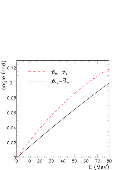
Figure 1: Left: The energy dependence of the changes in the neutrino mixing angles during the passage through vacuum, mantle and core. Right: The energy dependence of the magnitude of $\bar{A_{i}}$’s in Eq. (8).

We observe that the low-frequency component $\bar{A}_{0}$, that does not contribute to the Earth effects, is the largest in magnitude. Among the terms relevant for the Earth effects there are three dominant frequencies, corresponding to the first three terms in the summation in Eq. (8). The fourth term is subleading and the rest are too suppressed to be of any significance. The right panel of Fig. 1 confirms that the first three terms have similar magnitudes, in particular $|\bar{A}_{1}|\approx|\bar{A}_{2}|$, whereas the others are significantly suppressed for all the energies relevant for SN neutrinos. We expect the first three terms to give rise to three dominant peaks in the Fourier spectrum of the inverse energy spectrum. Note that since ${\overline{\Delta m^{2}_{c}}}\approx{\overline{\Delta m^{2}_{m}}}\approx\Delta m^{2}_{\odot}$ to within 20% in the relevant parameter range, the positions of these peaks are also known once the distance traversed through the Earth is known, independently of the primary neutrino spectra. This distance can be determined with sufficient precision even if the SN is optically obscured using the pointing capability of neutrino detectors [16].

3 Peaks in the power spectrum of $\mathbf{{\bar{\nu}_{e}}}$

3.1 Definitions

The neutrino signal is observed as a discrete set of events. The measured energy of these events is correlated to the neutrino energy via kinematics and detector properties. Then we define the power spectrum of $N$ detected events as

$$G(k)\equiv\frac{1}{N}\left|\sum_{i=1}^{N}e^{iky_{i}}\right|^{2}\,.$$ (10)

In the absence of Earth effect modulations, $G(k)$ is expected to have an average value of one for $k\raise 1.29167pt\hbox{$\;>$\kern-7.5pt\raise-4.73611pt\hbox{$\sim\;$}}40$ [13]. Earth effects introduce peaks in this power spectrum at specific frequencies, the identification of which correspond to the identification of the Earth effects.

Before defining an algorithm to analyze neutrino signals from a single SN, we perform a check of the analytical features derived in Sec. 2 with a realistic Monte Carlo simulation. For the time-integrated neutrino fluxes we assume distributions of the form [19]

$$F^{0}=\frac{\Phi_{0}}{E_{0}}\,\frac{(1+\alpha)^{1+\alpha}}{\Gamma(1+\alpha)}\left(\frac{E}{E_{0}}\right)^{\alpha}\exp\left[-(\alpha+1)\frac{E}{E_{0}}\right]\,,$$ (11)

where $F^{0}$ denotes the flux of a neutrino species emitted by the SN scaled appropriately to the distance traveled from the SN to Earth. Here $E_{0}$ is the average energy and $\alpha$ a parameter that relates to the width of the spectrum and typically takes on values 2.5–5, depending on the flavor and the phase of neutrino emission. The values of the total flux $\Phi_{0}$ and the spectral parameters $\alpha$ and $E_{0}$ are generally different for $\nu_{e}$, $\bar{\nu}_{e}$ and $\nu_{x}$, where $\nu_{x}$ stands for any of $\nu_{\mu,\tau}$ or $\bar{\nu}_{\mu,\tau}$.

• Model	$\langle E_{0}(\nu_{e})\rangle$	$\langle E_{0}({\bar{\nu}_{e}})\rangle$	$\langle E_{0}({\nu_{x}})\rangle$	$\frac{\Phi_{0}(\nu_{e})}{\Phi_{0}(\nu_{x})}$	$\frac{\Phi_{0}({\bar{\nu}_{e}})}{\Phi_{0}(\nu_{x})}$
  G	12	15	18	0.8	0.8
  L	12	15	24	2.0	1.6

Table 3: The parameters in the neutrino spectra models motivated from SN simulations of the Garching (G) group and the Livermore (L) group. We assume $\alpha=3$ for all neutrino species.

In order to study the model dependence, we consider two models that give very different predictions for the neutrino spectra. The first is motivated by the recent Garching calculation [20] that includes all relevant neutrino interaction rates, including nucleon bremsstrahlung, neutrino pair processes, weak magnetism, nucleon recoils and nuclear correlation effects. The second is the result from the Livermore simulation [21] that represents traditional predictions for flavor-dependent SN neutrino spectra that have been used in many previous analyses. The parameters of these models are shown in Table 3. To study the background, we use the mixing parameters of scenario B in Table 1 in which the Earth effects are absent.

For the Earth density profile we use a 5-layer approximation of the PREM model as parametrized in Ref. [15]. We start with a SN at 10 kpc and simulate the neutrino signal at a 32 kiloton scintillation detector and a megaton water Cherenkov detector. In both detectors, the neutrino signal is dominated by the inverse beta reaction ${\bar{\nu}_{e}}p\to ne^{+}$, while all other reactions have a negligible influence on the analysis below. The detector response is taken care of in the manner described in Refs. [7, 16]. The major difference between the scintillation and the water Cherenkov detector is that the energy resolution of the scintillation detector is roughly six times better than that of the Cherenkov detector. This compensates the size advantage of a megaton water Cherenkov detector.

3.2 Large scintillation detector

To start with, we consider the power spectrum resulting from averaging 1000 SN simulations. This eliminates the fluctuations in the background, and illustrates the characteristics of the peaks in a clear manner. The power spectrum at a 32 kt scintillation detector for different distances traveled through the Earth is shown in Fig. 2. The top panels use the Garching model whereas the bottom ones use the Livermore model. The left panels show three typical cases when the neutrinos traverse only the mantle, whereas the right panels represent the passage of neutrinos through the mantle as well as the core. Only inverse beta decay events have been taken into account. We have checked that the inclusion of the other reactions like the elastic scattering off electrons or the charged current reactions on carbon do not change the results. The neutral current reactions on carbon, although providing a large number of events, have been neglected, as the monoenergetic photon produced by the decay of the excited carbon could be tagged in such a detector [17].

• 

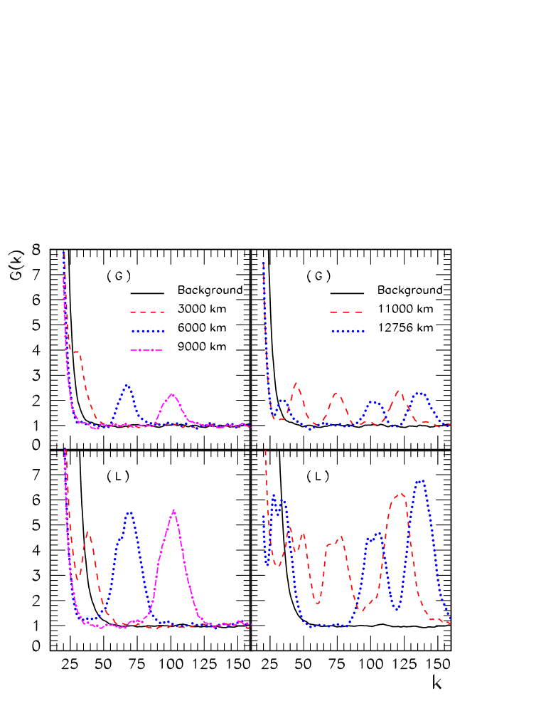
Figure 2: Averaged power spectra in the case of a large scintillator detector for different SN models, Garching (G) and Livermore (L), and distances travelled through the Earth.

The following observations may be made:

1. The average background approaches 1 for $k\raise 1.29167pt\hbox{$\;>$\kern-7.5pt\raise-4.73611pt\hbox{$\sim\;$}}40$, as expected [13]. The region $k\raise 1.29167pt\hbox{$\;<$\kern-7.5pt\raise-4.73611pt\hbox{$\sim\;$}}40$ is dominated by the “0-peak,” which is a manifestation of the low frequency terms in Eqs. (5) and (8). Note that the 0-peak in the background case is wider than that in the signal case. This is because the background case corresponds to the scenario B, which is also the one wherein there is a complete interchange of the ${\bar{\nu}_{e}}$ and ${\bar{\nu}_{x}}$ spectra. The energy of the detected ${\bar{\nu}_{e}}$ spectrum is thus higher, which results in a broader 0-peak.

2. When the neutrinos traverse only the mantle, only one peak appears at the expected value of $k_{m}$ that is proportional to the distance $L_{m}$ traveled through the mantle. For $L_{m}<3000$ km, the position of the peak lies at such low frequencies that it can hardly be distinguished from the 0-peak. This illustrates that neutrinos must travel a minimum distance through the Earth before the Earth effects become observable.

3. When the neutrinos travel also through the core, we observe three dominant peaks in each case, corresponding to $k_{1},k_{2}$ and $k_{3}$ in Eq. (8). We observe that, as the total distance traveled through the Earth increases,

   • the third peak moves to higher $k$, since $k_{3}\propto(L_{m}+L_{c})$.

   • the second peak, whose position is proportional to $(L_{m}/2+L_{c})$, also gets shifted towards higher $k$ as the increase in $L_{c}$ is larger than the decrease in $L_{m}/2$.

   • the first peak, on the other hand, moves to lower $k$ values, since as the trajectory of neutrinos approaches the center of the Earth, the distance traveled through the mantle decreases and so does the frequency of the lowest peak, $k_{1}\propto L_{m}/2$. This makes the detection of this peak harder at larger distances traveled through the Earth.

4. The model independence of the peak positions may be confirmed by comparing the top and bottom panels of Fig. 2. The peaks obtained with the Livermore model are stronger as a result of the larger difference between the ${\bar{\nu}_{e}}$ and ${\bar{\nu}_{x}}$ spectra in that model, which increases the value of $\Delta F^{0}$ in Eqs. (5) and (8). However, the positions of the peaks are the same as those obtained with the Garching model.

3.3 Megaton water Cherenkov detector

The energy resolution of a water Cherenkov detector is about a factor of six worse than that of a scintillation detector. This means that the energy spectrum is more “smeared out” and higher frequencies in the spectrum are more suppressed. This makes the peak identification more difficult, and even a detector of the size of Super-Kamiokande turns out not to be sufficient [13]. We show the power spectrum expected at a megaton water Cherenkov detector in Fig. 3 for the two SN models considered here and for different locations of the SN. Again we have only assumed the events from the inverse beta decay, since the contribution from other reactions is significantly smaller.

• 

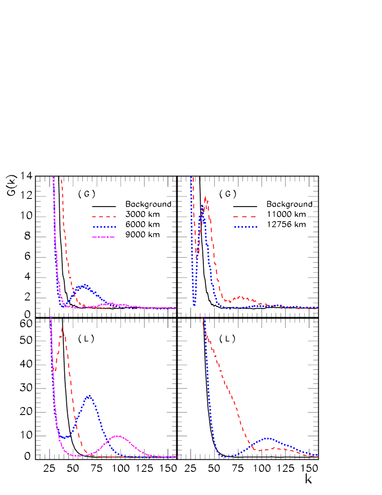
Figure 3: Same as the Fig. 2 but for the case of HK.

The following observations may be made from the power spectra:

1. The 0-peak is broader, which makes the averaged background approach one for larger values of $k$ ($k\simeq 50$) than in the case of the scintillation detector. This is because the energy smearing decreases the strengths of high frequency components and increases the strengths of low frequency components.

2. In the case of neutrino propagation only through the mantle, the peak shifts to higher $k$ as $L_{m}$ increases, as expected. However, the suppression of high frequencies tends to shift the peak locations to slightly lower $k$ values than at the scintillation detector. In addition, as the peak position moves to larger $k_{m}$, the strength of the peak decreases and the peak becomes harder to detect.

3. When the neutrinos traverse both the mantle and the core, it is observed that

   • the third peak among the expected three dominant ones, corresponding to $k_{3}\propto(L_{m}+L_{c})$, is highly suppressed due to large $k_{3}$ and is undetectable.

   • the other two peaks corresponding to $k_{1}\propto L_{m}/2$ and $k_{2}\propto(L_{m}/2+L_{c})$ have lower $k$ values, and are not as suppressed as the $k_{3}$ peak. Moreover, the $k_{1}$ peak is stronger than the $k_{2}$ one.

   • the $k_{1}$ peak moves to lower frequencies as the total distance traveled through the Earth increases. Beyond a certain distance, it merges with the background 0-peak and becomes undetectable.

4. The peak positions with the Garching and Livermore spectra are at nearly the same positions, though the extra feature of high $k$ suppression is observed to shift the peaks with the Garching model to slightly lower values of $k$ as compared to those with the Livermore model. The peaks with the Livermore model naturally have more strength than the ones with the Garching model.

4 Distinguishing the peaks from the background

4.1 An algorithm for peak identification

Though the analytic approximations seem to work well with the averaged power spectrum, the understanding of the statistical fluctuations within the signal from a single SN is crucial for the identification of the peaks. As observed in [13] and confirmed in Sec. 3, the average of the background power spectrum is indeed one for all values of $k$ after the dominant low frequency peak in the power spectrum dies out. As long as we are free of the influence of this low frequency peak, the area under the power spectrum between two fixed frequencies $k_{\rm min}$ and $k_{\rm max}$ is on an average $(k_{\rm max}-k_{\rm min})$. In the absence of Earth effects, this area will have a distribution centered around this mean. The Earth effect peaks tend to increase this area. If the area in a specific interval is found to be more than what mere background fluctuations can allow, the peak can be identified with confidence.

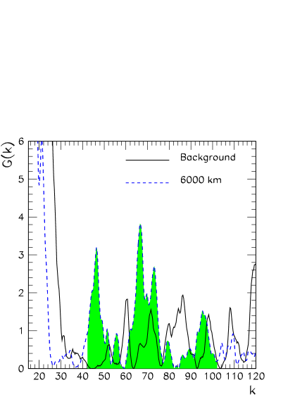
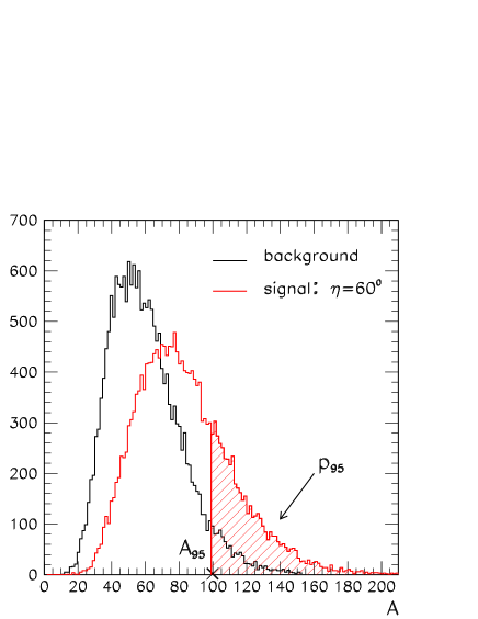
Figure 4: Left: Realistic spectrum from a single simulation. Right: Area distribution of the background (black) and the signal (red) obtained for a 32 kton scintillator detector and Garching model for $\eta=60$.

Since in the real world the presence of fluctuations in the signal will spoil any naive theoretical peak, we need to introduce a prescription to carry out the analysis.

1. Once we know the total distance traveled by the neutrinos through the Earth, we can calculate the position where the peak should lie. Instead of looking for the maximum in the height of the power spectrum, we consider a more robust observable, namely the area around the position of the peak, as illustrated in Fig. 4. When only one peak centered at $k_{m}$ is expected, we consider the interval $k_{m}\pm\Delta k$ with $\Delta k=30$, roughly the expected width of the peak. In order to avoid the 0-peak contamination we set a lower limit at $k=40$ ($k=50$) for the scintillator (water Cherenkov) detector. When the neutrinos also cross the Earth core, multiple peaks are present and we measure the area from $k=40$ until $k=160$ in such cases.

2. The next step is to analyze the statistical significance of the result obtained. For this purpose we compare the value of the measured area with the distribution of the area in the case of no Earth matter effects. Since the different frequencies are not uncorrelated, the background distribution is not simply Gaussian centered at $A_{\rm av}=(k_{\rm max}-k_{\rm min})$ and with width $\sqrt{k_{\rm max}-k_{\rm min}}$. Therefore, we perform a Monte Carlo analysis of the background case and calculate the exact distribution with which one can compare the actual area measured. We illustrate this in the right panel of Fig. 4, where the black curve shows the area distribution of the background. The confidence level of peak identification may then be defined as the fraction of the area of the background distribution that is less than the actual area measured. We denote the area corresponding to $\alpha$% C.L. by $A_{\alpha}$. Figure 4 also shows $A_{95}\approx 100$, the area corresponding to a peak identification with 95% confidence.

4.2 Quantifying the efficiency of the algorithm

Since the peak identification algorithm is statistical in nature, it is worthwhile to have an idea of the probability with which a peak can be identified with a given confidence. This probability clearly depends on the distance traveled by the neutrinos through the Earth, which in turn is determined by the location of the SN in the sky. We parameterize the SN location by the nadir angle $\eta$ of the SN direction at the detector.

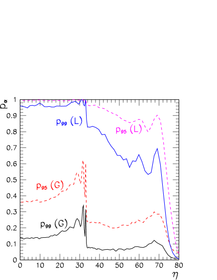
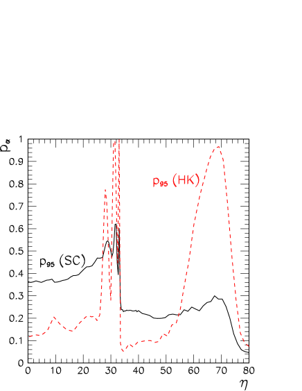
Figure 5: Left: Comparison of $p_{95}$ and $p_{99}$ for the Garching (G) and Livermore (L) SN models in a 32 kton scintillator detector. Right: Comparison of $p_{95}$ in this large scintillator detector (SC) and in the case of a megaton water Cherenkov (HK), for the Garching model.

We simulate the area distribution for the “signal” using the neutrino mixing scenarios that allow Earth effects and compare it with the background distribution. The probability $p_{\alpha}$ of peak identification at $\alpha$% C.L. is the fraction of the area of the signal distribution above $A_{\alpha}$. In Fig. 4, it has been indicated with the red-hashed region. In Fig. 5 we show $p_{95}$ and $p_{99}$ as a function of $\eta$ in the case of a scintillation detector, for the two SN models considered. An increase in the distance traveled through the Earth corresponds to a decrease in $\eta$. The passage through the core corresponds to $\eta<33^{\circ}$. One can see that the presence of the core enhances the chances of detecting the Earth matter effects. The probability is higher at values of $\eta$ close to the boundary between the mantle and the core because the three peaks are clearly visible. The oscillation pattern arising at this region stems from the interference of the first two peaks in the spectrum, whose positions at this point differ only by $\phi_{c}\propto L_{c}$. As the distance traveled by the neutrinos through the core increases, $p_{\alpha}$ decreases, the reason being the approach of the first peak to the lower limit frequency, $k\simeq k_{\rm min}$, and its eventual disappearance.

As expected, the chances of peak identification are also higher when the primary spectra of ${\bar{\nu}_{e}}$ and ${\bar{\nu}_{x}}$ differ more. As shown in Fig. 5, the Livermore model predicts much larger chances of a successful peak identification.

In the right panel of Fig. 5, we assume the Garching model and compare the results obtained with a 32 kton scintillator detector and a megaton water Cherenkov detector. In the latter case, as neutrinos travel more and more distance in the mantle the peak moves to higher $k$ values, and due to the high $k$ suppression as described in Sec. 3.3, the efficiency of peak identification decreases. However, when the neutrinos start traversing the core, additional low $k$ peaks are generated and the efficiency increases again.

One of the features of this algorithm is its robustness. However in some cases it turns out to be very conservative. For instance, if we have a look at the megaton water Cherenkov, the peaks at the lowest frequencies are almost eaten-up by the 0-peak of the background when the neutrinos cross the Earth core, cf. Fig. 3. Setting $k_{\min}=50$ as the lower limit of the area integration results therefore in a loss of considerable amount of information under these conditions. In this particular case it is possible to optimize the efficiency of the method by choosing a floating lower cut: instead of considering a fixed value, $k_{\rm min}=50$, as the lower limit for the area integration, one defines $k_{\rm min}$ as the frequency at which the spectrum has the first minimum after neglecting the effect of spurious fluctuations. With this modified prescription one can again compare the area distribution for the background and that of the signal, and calculate a new $p_{\alpha}$. We have checked this method for both the scintillator and the water Cherenkov detector. For the former the improvement is not relevant. The reason is that the second and third peaks contribute significantly to the signal. So, even when the first peak disappears behind the 0-peak of the background for fixed lower cut-off, the loss of information is not important. However in the case of a water Cherenkov detector the efficiency is significantly enhanced for paths traversing the Earth core as can be seen in Fig. 6. Due to the suppression of the peaks located at higher frequencies only the first peak contributes significantly to the signal. However for trajectories involving small $\eta$ this peak is centered at very low frequencies, almost completely hidden by the 0-peak of the background. Under this situation if one allows the lower bound to shift to smaller frequencies the whole peak contributes to the signal, and therefore the probability to see the Earth matter effects increases. On the other hand when the neutrinos only cross the mantle the location of the unique peak is mostly at $k>k_{\rm min}=50$. Therefore, this modified prescription does not help much to improve the efficiency to observe the modulation of the neutrino spectra due to the Earth matter effects.

• 

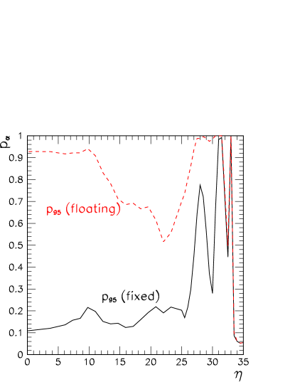
Figure 6: Comparsion of $p_{95}$ for two different methods of integration, with fixed and floating lower limit, in the case of a megaton water Cherenkov detector and the Garching model.

5 Summary and conclusions

When neutrinos coming from a core-collapse supernova pass through the Earth before arriving at the detector, the spectra may get modified due to the Earth matter effects. The presence or absence of these effects can distinguish between different neutrino mixing scenarios. We have seen that these Earth matter effects on supernova neutrinos can be identified at a single detector through peaks in the Fourier transform of their “inverse energy” spectrum. The position of these peaks are independent of the initial neutrino fluxes and spectral shapes.

We have performed an analytical study of the positions and the strengths of the frequencies that characterize the inverse-energy spectrum of the neutrinos for different neutrino trajectories through the Earth. In the case that the SN neutrinos only traverse the mantle a single peak shows up in the power spectrum. In contrast we have observed that if both the mantle and the core are crossed before the neutrinos reach the detector as many as seven distinct frequencies are present in the inverse energy spectrum. However only three peaks are dominant in the power spectrum. This increase in the number of expected peaks leads to an easier identification of the Earth matter effects.

In order to illustrate the qualitative features of the present analysis we have considered the power spectrum resulting from averaging 1000 SN simulations for different SN models and different detector capabilities. In particular we have assumed a 32 kton scintillator detector and a megaton water Cherenkov detector. We have shown how the energy resolution turns out to be crucial in detecting the modulation introduced in the neutrino spectra by the Earth matter effects. First, the better resolution of the scintillator detector compensates for the larger water Cherenkov detector size. On the other hand, the worse energy resolution in water Cherenkov detectors does not only imply the need of a larger volume but also suppresses significantly the peaks at higher frequencies, in contrast to the case of scintillator detectors.

We have considered two different SN models as an illustration of the current uncertainties in the initial fluxes. We have observed that the strength of the peaks is larger in those SN models with bigger differences between $\bar{\nu}_{e}$ and $\bar{\nu}_{\mu}$ spectra. However, we have found that the position of the peaks is model independent. Therefore their identification serves as a clear signature of the Earth matter effects on SN neutrinos, which in turn can help to discard the neutrino mass scheme with inverted mass hierarchy and $\sin^{2}\Theta_{13}\raise 1.29167pt\hbox{$\;>$\kern-7.5pt\raise-4.73611pt\hbox{$\sim\;$}}10^{-3}$.

We have introduced a simple algorithm to identify the peaks in the presence of background fluctuations. This method is based on the integration of the area around the expected position of the peak. By comparing the area distribution without and with the spectral modulations induced by the Earth matter effects we have analyzed the statistical significance of the result. As expected the presence of the core as well as a larger difference in the initial spectra enhance the probability of identifying the Earth effects. We have also presented a variation of the algorithm which improves its efficiency significantly in the case of a water Cherenkov detector for neutrino trajectories passing through the core. Therefore we believe that more efficient algorithms could be developed. The results we presented should be considered therefore as conservative lower limits.

References

References

- [1] C. Lunardini and A. Y. Smirnov, “Neutrinos from SN1987A, Earth matter effects and the LMA solution of the solar neutrino problem,” Phys. Rev. D 63 (2001) 073009 [hep-ph/0009356].
- [2] M. Kachelrieß, A. Strumia, R. Tomàs and J. W. Valle, “SN1987A and the status of oscillation solutions to the solar neutrino problem,” Phys. Rev. D 65 (2002) 073016 [hep-ph/0108100].
- [3] H. Minakata and H. Nunokawa, “Inverted hierarchy of neutrino masses disfavored by supernova 1987A,” Phys. Lett. B 504 (2001) 301 [hep-ph/0010240].
- [4] V. Barger, D. Marfatia and B. P. Wood, “Supernova 1987A did not test the neutrino mass hierarchy,” Phys. Lett. B 532 (2002) 19 [hep-ph/0202158].
- [5] A. S. Dighe and A. Y. Smirnov, “Identifying the neutrino mass spectrum from the neutrino burst from a supernova,” Phys. Rev. D 62 (2000) 033007 [hep-ph/9907423].
- [6] C. Lunardini and A. Y. Smirnov, “Probing the neutrino mass hierarchy and the 13-mixing with supernovae,” JCAP 0306 (2003) 009 [hep-ph/0302033].
- [7] A. S. Dighe, M. Kachelrieß, G. G. Raffelt and R. Tomàs, in preparation.
- [8] A. S. Dighe, “Earth matter effects on the supernova neutrino spectra,” hep-ph/0106325.
- [9] C. Lunardini and A. Y. Smirnov, “Supernova neutrinos: Earth matter effects and neutrino mass spectrum,” Nucl. Phys. B 616 (2001) 307 [hep-ph/0106149].
- [10] K. Takahashi and K. Sato, “Earth effects on supernova neutrinos and their implications for neutrino parameters,” Phys. Rev. D 66, 033006 (2002) [hep-ph/0110105].
- [11] M. Lindner, T. Ohlsson, R. Tomàs and W. Winter, “Tomography of the earth’s core using supernova neutrinos,” Astropart. Phys. 19 (2003) 755 [hep-ph/0207238].
- [12] A. S. Dighe, M. T. Keil and G. G. Raffelt, “Detecting the neutrino mass hierarchy with a supernova at IceCube,” JCAP 0306 (2003) 005 [hep-ph/0303210].
- [13] A. S. Dighe, M. T. Keil and G. G. Raffelt, “Identifying earth matter effects on supernova neutrinos at a single detector,” JCAP 0306 (2003) 006 [hep-ph/0304150].
-
[14]
http://int.phys.washington.edu/int_talk/WorkShops/TAUP03/Parallel/People/Oberauer_L/
LENA-Oberauer.pdf - [15] E. Lisi and D. Montanino, “Earth regeneration effect in solar neutrino oscillations: An analytic approach,” Phys. Rev. D 56 (1997) 1792 [hep-ph/9702343].
- [16] R. Tomàs, D. Semikoz, G. G. Raffelt, M. Kachelrieß and A. S. Dighe, “Supernova pointing with low- and high-energy neutrino detectors,” hep-ph/0307050.
- [17] L. Cadonati, F. P. Calaprice and M. C. Chen, “Supernova neutrino detection in Borexino,” Astropart. Phys. 16 (2002) 361 [hep-ph/0012082].
- [18] J. F. Beacom and M. R. Vagins, “GADZOOKS! Antineutrino spectroscopy with large water Cherenkov detectors,” hep-ph/0309300.
- [19] M. T. Keil, G. G. Raffelt and H. T. Janka, “Monte Carlo study of supernova neutrino spectra formation,” Astrophys. J. 590 (2003) 971 [astro-ph/0208035].
- [20] G. G. Raffelt, M. T. Keil, R. Buras, H. T. Janka and M. Rampp, “Supernova neutrinos: Flavor-dependent fluxes and spectra,” astro-ph/0303226.
- [21] T. Totani, K. Sato, H. E. Dalhed and J. R. Wilson, “Future detection of supernova neutrino burst and explosion mechanism,” Astrophys. J. 496, 216 (1998) [astro-ph/9710203].