Testing the running of the cosmological constant with Type Ia Supernovae at high z

Abstract:

Within the Quantum Field Theory context the idea of a “cosmological constant” (CC) evolving with time looks quite natural as it just reflects the change of the vacuum energy with the typical energy of the universe. In the particular frame of Ref. [31], a “running CC” at low energies may arise from generic quantum effects near the Planck scale, $M_{P}$, provided there is a smooth decoupling of all massive particles below $M_{P}$. In this work we further develop the cosmological consequences of a “running CC” by addressing the accelerated evolution of the universe within that model. The rate of change of the CC stays slow, without fine-tuning, and is comparable to $H^{2}\,M_{P}^{2}$. It can be described by a single parameter, $\nu$, that can be determined from already planned experiments using SNe Ia at high z. The range of allowed values for $\nu$ follows mainly from nucleosynthesis restrictions. Present samples of SNe Ia can not yet distinguish between a “constant” CC or a “running” one. The numerical simulations presented in this work show that SNAP can probe the predicted variation of the CC either ruling out this idea or confirming the evolution hereafter expected.

1 Introduction

The Standard Cosmological Model fits our universe, in the large, into an homogeneous and isotropic Friedmann-Lemaître-Robertson-Walker (FLRW) cosmological type  [1]. Its 4-curvature is determined from the various contributions to its total energy density, namely in the form of matter, radiation and cosmological constant.

Evidence for a dominant content of energy in the form of cosmological constant was found by tracing the rate of expansion of the universe along z with high–z Type Ia supernovae [2, 3]. This measurement combined with the measurements of the total energy density $\Omega_{T}^{0}$ from the CMB anisotropies [4, 5], indicates that $\Omega_{\Lambda}^{0}\sim 70\%$ of the critical energy density of the universe is cosmological constant (CC) or a dark energy candidate with a similar dynamical impact on the evolution of the expansion of the universe. The matter content, on the other hand is dominated by the dark matter, whose existence is detected by dynamical means [1], and amounts to $\Omega_{M}^{0}\sim 30\%$ of the critical density.

The CC value found from Type Ia supernovae at high z [2, 3] is:

$$\Lambda_{0}=\Omega_{\Lambda}^{0}\,\rho_{c}^{0}\simeq 6\,h_{0}^{2}\times 10^{-47}\,GeV^{4}\,.$$ (1)

Here $\rho_{c}^{0}\simeq\left(3.0\,\sqrt{h_{0}}\times 10^{-12}\,GeV\right)^{4}$ is the present value of the critical density, and $h_{0}\sim 0.7\pm 0.1$ sets the typical range for today’s value of Hubble’s constant $H_{0}\equiv 100\;(Km/sec\,Mpc)\;h_{0}$. In the context of the Standard Model (SM) of electroweak interactions, this measured CC should be the sum of the original vacuum CC in Einstein’s equations, $\Lambda_{vac}$, and the induced contribution from the vacuum expectation value of the Higgs effective potential, $\Lambda_{ind}=\langle V_{\rm eff}\rangle$:

$$\Lambda=\Lambda_{vac}+\Lambda_{ind}\,.$$ (2)

It is only this combined parameter that makes physical sense, whereas both $\Lambda_{vac}$ and $\Lambda_{ind}$ remain individually unobservable. From the current LEP 200 numerical bound on the Higgs boson mass, $\,M_{H}>114.1\,GeV$ [6], one finds $\,\,\,\left|\Lambda_{ind}\right|=(1/8)M_{H}^{2}\,v^{2}>1.0\times 10^{8}\,GeV^{4}$, where $v\simeq 246\,GeV$ is the vacuum expectation value of the Higgs field. Clearly, $\left|\Lambda_{ind}\right|$ is $55$ orders of magnitude larger than the observed CC value (1). Such discrepancy, the so-called “old” cosmological constant problem [7, 8], manifests itself in the necessity of enforcing an unnaturally exact fine tuning of the original cosmological term $\Lambda_{vac}$ in the vacuum action that has to cancel the induced counterpart $\,\Lambda_{ind}$ within a precision (in the SM) of one part in $\,10^{55}$.

The measured CC remains very small as compared to the huge CC value predicted in the SM of Particle Physics. Actually, if the physical value of the CC would conform with that one predicted in the SM, the curvature of our universe would be so high that the Special Theory of Relativity could not be a solution to Einstein equations to any reasonable degree of approximation. Therefore, the SM prediction of the CC violently contradicts our experience, whereas the small measured value (1) is perfectly compatible with it.

The Cosmological Constant Problem (CCP) is a fundamental problem. It is most likely related to the delicate interplay between Gravity and Particle Physics, and it has become one of the main poles of attention [7, 8]. All attempts to deduce the small value of the cosmological constant from a sound theoretical idea ended up with the necessity of introducing severe fine-tuning. This concerns also, unfortunately, the use of supersymmetry and string theory (see e.g. [9, 10]). In this respect we recall that, for a realistic implementation of the existing versions of M-Theory, one would like to have a negative (or at least vanishing) cosmological constant in the remote future, such that it does not prevent the construction of the asymptotic S-matrix states in accelerated universes [11]. Since the presently observed value of the CC is positive, there is the hope that a variable cosmological term may solve this problem.

There is a permanently growing flux of proposals concerning the CCP. On the first place there is the longstanding idea of identifying the dark energy component with a dynamical scalar field [12, 13]. More recently this approach took the popular form of a “quintessence” field slow–rolling down its potential [14]. This proposal has, on its own, given rise to a wide variety of models [15, 16]. Extended models of this kind (“k–essence”) are also based on scalar fields but with a non-canonical kinetic energy [17]. The main advantage of the quintessence models is that they could explain the possibility of a variable vacuum energy. This may become important in case such variation will be someday detected in the observations. Recently other approaches have appeared in which the dark energy is mimicked by new gravitational physics [18]. From the point of view of the CCP, all these approaches lead to the introduction of either a very small parameter or a very high degree of fine-tuning. In another, very different, vein the possibility to accept the observed value of the CC within the context of a many world pool is offered by the anthropic proposal [19]. Let us finally mention the intriguing proposal of non-point-like gravitons at sub-millimeter distances suggested in [20], or the possibility of having multiply degenerate vacua [21].

When assessing the possibility to have variable dark energy, other no less respectable possibilities should be taken into account. In a series of recent papers [22, 23], the idea has been put forward that already in standard Quantum Field Theory (QFT) one would not expect the CC to be constant, because the Renormalization Group (RG) effects may shift away the prescribed value, in particular if the latter is assumed to be zero. Thus, in the RG approach one takes a point of view very different from e.g. the quintessence proposal, as we deal all the time with a “true” cosmological term. It is however a variable one, and therefore a time-evolving, or redshift dependent: $\Lambda=\Lambda(z)$. Although we do not have a QFT of gravity where the running of the gravitational and cosmological constants could ultimately be substantiated, a semiclassical description within the well established formalism of QFT in curved space-time (see e.g. [24, 25]) should be a good starting point. From the RG point of view, the CC becomes a scaling parameter whose value should be sensitive to the entire energy history of the universe – in a manner not essentially different to, say, the electromagnetic coupling constant. One of the main distinctions between our approach and all kinds of quintessence models is that these models imply the introduction of a phenomenological equation of state $p_{\chi}=w\,\rho_{\chi}$ for the scalar field $\chi$ mimicking the CC, where $w$ is a negative index (smaller than $-1/3$). Whether constant or variable, a “true” cosmological parameter has, instead, no other equation of state associated to it apart from the exact $w=-1$ one.

Attempts to apply the RG for solving the CC problem have been made earlier [26, 27]. The canonical form of renormalization group equation (RGE) for the $\Lambda$ term at high energy is well known – see e.g. [25, 28]. However, at low energy decoupling effects of the massive particles may change significantly the structure of this RGE, with important phenomenological consequences. This idea has been retaken recently by several authors from various interesting points of view [22, 23, 29, 30]. However, it is not easy to achieve a RG model where the CC runs smoothly without fine tuning at the present epoch. In Ref. [31, 32] a successful attempt in this direction has been made, which is based on possible quantum effects near the Planck scale. At the same time, the approximate coincidence of the observed $\Lambda$ and the matter density, $\ \Omega_{\Lambda}^{0}\sim\Omega_{M}^{0}\,$, i.e. the “new” CC problem, or “time coincidence problem” [7, 8] can be alleviated in this framework if we assume the standard (viz. Appelquist-Carazzone [33]) form of the low-energy decoupling for the massive fields.

In the present paper we elaborate on this idea further. We develop a semiclassical FLRW model whose running CC is driven smoothly, without fine tuning, due to generic quantum effects near the Planck scale. We show that, due to the decoupling phenomenon, the low-energy effects (in particular the physics from the SM scale) are irrelevant for the CC running, and so the approximate coincidence between $\Omega_{M}^{0}$ and $\Omega_{\Lambda}^{0}$ is not tied to any particular epoch in the history of the universe. Furthermore, the new effects imply deviations from the standard cosmological equations due to quantum effects. Our “renormalized” FLRW model provides a testable framework that can be thoroughly checked from SNAP data on Type Ia supernovae at very high z – see [34, 35] and references in [36]. If these experiments detect a $z$-dependence of the CC similar to that predicted in our work, we may suspect that some relevant physics is going on just below the Planck scale. Alternatively, if they find a static CC, this might imply the existence of a desert in the particle spectrum near the Planck scale.

The structure of the paper is as follows. In the next section we compare constant versus variable CC models. In Section 3 we present our variable CC model based on the Renormalization Group. In Section 4 we solve the FLRW cosmologies with running CC. In Section 5 we study the numerical behaviour of these cosmologies, and the predicted deviations from the standard FLRW expectations. In Section 6, we introduce the magnitude-redshift relation for the analysis of the SNe Ia. In Section 7 we perform the simulations on the SNAP data in order to test the sensitivity with which the features of the new model can be determined. In the last section we draw our conclusions. Two appendices are included at the end: one to discuss some technical issues inherent to our QFT framework, the other providing some background related to the statistical analysis.

2 Constant versus variable cosmological term

The cosmological constant enters the Hilbert-Einstein (HE) action as follows

$$S_{HE}=-\int d^{4}x\sqrt{-g}\,\left(\,\frac{1}{16\pi G}\,R+\Lambda_{vac}\,\right)\,.$$ (3)

It is well-known that renormalizability requires that this effective action should be extended with a number of higher derivative terms [24, 25]:

$$S_{vac}=\int d^{4}x\sqrt{-g}\,\Big{\{}\,a_{1}R^{2}_{\mu\nu\alpha\beta}+a_{2}R^{2}_{\mu\nu}+a_{3}R^{2}+a_{4}{\square}R-\frac{1}{16\pi G_{vac}}\,R-\Lambda_{vac}\Big{\}}\,.$$ (4)

The phenomenological impact of the higher derivative terms in this action is negligible at present, and therefore it suffices to use the low-energy action (3). However, the presence of the parameter $\Lambda_{vac}$ is as necessary as any one of these higher derivative terms to achieve a renormalizable QFT in curved space-time .

The vacuum CC itself, $\Lambda_{vac}$, is not the physical (observable) value of the cosmological constant. By definition the physical CC is the parameter $\Lambda$ entering the Friedmann-Lemaître equation:

$$H^{2}\equiv\left(\frac{\dot{a}}{a}\right)^{2}=\frac{8\pi\,G_{N}}{3}\left(\rho+\Lambda\right)-\frac{k}{a^{2}}\,,$$ (5)

where $H$ is the expansion parameter (Hubble’s “constant”). This $\Lambda$ should be the sum (2). While the homogeneous and isotropic FLRW cosmologies do not allow spatial gradients of $\Lambda$, they do not forbid the possibility that $\Lambda$ may be a function of the cosmological time: $\Lambda=\Lambda(t)$. In this case the Einstein field equations associated to the action (3) read

$$R_{\mu\nu}-\frac{1}{2}g_{\mu\nu}R=-8\pi G_{N}\ \tilde{T}_{\mu\nu}\,,$$ (6)

where $\tilde{T}_{\mu\nu}$ is given by $\tilde{T}_{\mu\nu}\equiv T_{\mu\nu}+g_{\mu\nu}\,\Lambda(t)$, $T_{\mu\nu}$ being the ordinary energy-momentum tensor associated to matter and radiation. By the Bianchi identities, it follows that $\Lambda$ is a constant if and only if the ordinary energy-momentum tensor is individually conserved ($\bigtriangledown^{\mu}\,{T}_{\mu\nu}=0$). In particular, $\Lambda$ must be a constant if ${T}_{\mu\nu}$ is zero (e.g. during inflation).

Modeling the expanding universe as a perfect fluid with velocity $4$-vector field $U^{\mu}$, we have

$$T_{\mu\nu}=-p\,g_{\mu\nu}+(\rho+p)U^{\mu}U^{\nu}\,,$$ (7)

where $p$ is the isotropic pressure and $\rho$ is the proper energy density of matter. Clearly $\tilde{T}_{\mu\nu}$ takes the same form as (7) with $\rho\rightarrow\tilde{\rho}=\rho+\Lambda\,,\ \ \ p\rightarrow\tilde{p}=p-\Lambda$. Using the FLRW metric

$$ds^{2}=dt^{2}-a^{2}(t)\left(\frac{dr^{2}}{1-k\,r^{2}}+r^{2}\,d\theta^{2}+r^{2}\,\sin^{2}\theta\,d\phi^{2}\right)\,,$$ (8)

we can compute explicitly the local energy-conservation law $\bigtriangledown^{\mu}\,\tilde{T}_{\mu\nu}=0$. The result is the old Bronstein’s equation [37] allowing transfer of energy between ordinary matter and the dark energy associated to the $\Lambda$ term:

$$\dot{\Lambda}+\dot{\rho}+3\,H\,(\rho+p)=0\,.$$ (9)

We see that the most general local energy conservation law (or equation of continuity) involves both the time evolution of $\rho$ and that of $\Lambda$. For a truly constant CC, then $\dot{\Lambda}=0$, and we recover of course the standard conservation law $\,\,\dot{\rho}+3\,H\,(\rho+p)=0$. Equations (5) and (9) constitute two independent counterparts for constructing FLRW cosmologies with variable $\Lambda$. The dynamical equation for the scale factor is

$$\ddot{a}=-\frac{4\pi}{3}G_{N}\,(\tilde{\rho}+3\,\tilde{p})\,a=-\frac{4\pi}{3}G_{N}\,(\rho+3\,p-2\,\Lambda)\,a\,,$$ (10)

but it is not independent from the previous two. In the matter era $p=0$, and Eq. (10) shows that unless $|\Lambda|$ is much smaller than $\rho$, a positive $\Lambda$ eventually implies accelerated expansion – as in fact seems to be the case for our universe [2, 3].

It should be clear that our approach based on a variable CC departs from all kind of quintessence-like approaches, in which some slow–rolling scalar field $\chi$ substitutes for the CC. In these models, the dark energy is tied to the dynamics of $\chi$, whose phenomenological equation of state is defined by $p_{\chi}=w\,\rho_{\chi}$. The term $-2\,\Lambda$ on the r.h.s. of Eq. (10) must be replaced by $\rho_{\chi}+3\,{p}_{\chi}=(1+3\omega)\rho_{\chi}$. In order to get accelerated expansion in an epoch characterized by $p=0$ and $\rho\rightarrow 0$ in the future, we must require $-w_{-}\leq w\leq-1/3$, where usually $w_{-}\geq-1$ in order to have a canonical kinetic term for $\chi$. However, one cannot completely exclude “phantom matter-energy” ($w_{-}<-1$) and generalizations thereof [38]. Present data suggest the interval $-1.38\leq w\leq-0.82$ at $95\%\,$ C.L. [39]. Although $p_{\chi}$ and $\rho_{\chi}$ are related to the energy-momentum tensor of $\chi$, the dynamics of this field is unknown because the quintessence models do not have an explanation for the value of the CC. Therefore, the barotropic index $w$ is not known from first principles. In particular, one cannot exclude it may have a redshift dependence, which can be parametrized in various ways as follows:

$$\frac{p_{\chi}}{\rho_{\chi}}\equiv w=w_{0}+w_{1}z+{\cal O}(z^{2})=w_{0}+w_{a}(1-a)+{\cal O}((1-a)^{2})\,,$$ (11)

where $z+1=1/a$. Finding a non-vanishing value of $w_{1}$ ($w_{a}$) implies a redshift evolution of the equation of state for the $\chi$ field  [5]. The difficulties to measure $w_{1}$ are well-known, see e.g. [40].

Quite in contrast to that scenario, since our variable CC is a “true” cosmological parameter, the only possible equation of state for the CC term is $p=-\Lambda$, whether it is a true constant or it is a parameter that evolves with the cosmological time. In our case the CC is indeed a variable one, and its variation is attributed to potential quantum effects linked to physics near the Planck scale, as will be explained in the next section.

3 Renormalization group and cosmological constant

The possibility of a cosmological model with a time-dependent $\Lambda$ as presented in the previous section is very generic. However, the two differential equations (5) and (9) cannot be solved unless a third equation involving $\Lambda$ is called for. The third equation admits many formulations, even at the classical level . However, a particularly interesting implementation occurs when the time dependence has its prime origin in the quantum field theory notion of Renormalization Group running [22, 23]. It means that the Hilbert-Einstein action (3) is treated semiclassically and one introduces an equation for the running cosmological constant. Although this can be done in several ways, a consistent formulation of the approach has been presented in [22] within the well established formalism of QFT in curved space-time (see e.g. [24, 25]). From simple dimensional analysis, and also from dynamical features to be discussed below, the RGE for the physical CC may take in principle the generic form [22, 29]

$$\frac{d\Lambda}{d\ln\mu} =\frac{1}{(4\pi)^{2}}\left(\sum_{i}\,A_{i}\,m_{i}^{4}+\mu^{2}\sum_{j}\,B_{j}M_{j}^{2}\,\,+\mu^{4}\sum_{j}\,C_{j}+\mu^{6}\sum_{j}\frac{\,D_{j}}{M_{j}^{2}}\,\,+...\right)$$ (12)

$$\equiv\,\sum_{n=0}^{\infty}\,\sum_{i}\,\alpha_{in}\,{\cal M}_{i}^{4}\,\left(\frac{\mu}{{\cal M}_{i}}\right)^{2n}\,\equiv\beta_{\Lambda}({\cal M}_{i},\mu/{\cal M}_{i}).$$

where the sums are taken over all massive fields; $\,A,B,C,D,...\,$ are constant coefficients, and $\mu$ is the energy scale associated to the RG running. We assume that $\mu$ is of the order of some physical energy-momentum scale characteristic of the cosmological processes, and can be specified in different ways (see below). In our model we assume that $\mu$ is given by the typical energy-momentum of the cosmological gravitons, namely $\mu=H$, which is of order $R^{1/2}$. The r.h.s. of (12) defines the $\beta_{\Lambda}$-function for $\Lambda$, which is a function of the masses and in general also of the ratios of the RG scale and the masses.

In the equation above the masses of the various degrees of freedom (d.o.f.) are represented by $m_{i}$ and $M_{j}$. Here we distinguish between the active (or “light”) d.o.f. at the scale $\mu$, namely those satisfying $\mu\gg m_{i}$ and contributing to the $\beta_{\Lambda}$-function in the form $\sim m_{i}^{4}$, from the “decoupled” (or “heavy”) d.o.f. which satisfy $\mu\ll M_{j}$ and yield the remaining terms in the series expansion of $\beta_{\Lambda}$ in powers of $\mu/M_{j}\ll 1$. As can be seen, all the terms in $\beta_{\Lambda}$ are of the form $\mu^{2n}\,{\cal M}_{i}^{4-2n}\ (n=0,1,2,3...)$ where ${\cal M}_{i}=m_{i}$ for $n=0$ and ${\cal M}_{i}=M_{i}$ for $n\geq 1$. The $n=0$ terms correspond precisely to the active d.o.f. contributing the full fourth power of their masses. The coefficients $A_{i}$ for these terms are known in the ultraviolet (UV) regime because they must coincide, in any mass-dependent renormalization framework, with their values in the Minimal Subtraction (MS) scheme [43, 44]. In this regime the $\beta_{\Lambda}$-function depends only on the masses of the active degrees of freedom, and not on the ratios $\mu/M_{i}$ of the RG scale and the heavy masses. For particles $i=1,2,3,...$ of masses $m_{i}$ and spins $J_{i}$ one finds [22]:

$$A_{i}=(-1)^{2J_{i}}(J_{i}+1/2)\,n_{J_{i}}\,N_{c}\,,$$ (13)

with $n_{\{0,1,1/2\}}=(1,1,2)$ and $N_{c}=1,3$ for uncolored and colored particles respectively. The remaining terms in (12) “decouple” progressively faster as we move from $n=1,2,3,...\$

Notice that dimensional analysis is not enough to explain the most general structure of $\beta_{\Lambda}$. The fact that only even powers of $\mu$ are involved stems from the covariance of the effective action. Indeed, the odd-powers of $\mu$ cannot appear after integrating out the higher derivative terms, as they must appear bilinearly in the contractions with the metric tensor. In particular, covariance forbids the terms of first order in $\mu$. As a result the expansion must start at the $\mu^{2}$-order. On the other hand, the structure for the $n\geq 1$ terms associated to the coefficients $B$, $C$, … in (12) is dictated by the the Appelquist-Carazzone (AC) decoupling theorem [33, 43]. Thus, when applying the AC theorem in its very standard form to the computation of $\beta_{\Lambda}$, the decoupling does still introduce inverse power suppression by the heavy masses (those satisfying $M_{j}\gg\mu$), but since the $\beta_{\Lambda}$-function itself is proportional to the fourth power of these masses it eventually entails a decoupling law $1/M^{2n-4}_{j}$, and so the $n=1$ and $n=2$ terms do not decouple in the ordinary sense whereas the $n\geq 3$ terms do, i.e. only the latter start getting (increasingly higher) inverse power suppression by the heavy masses. The upshot is that, strictly speaking, the truly decoupling terms in $\beta_{\Lambda}$ (in the sense used when applying the AC theorem to the ordinary SM interactions) commence at $n=3$ and above. In contrast, the $n=2$ terms are constant (independent of the masses) and the $n=1$ terms acquire the peculiar structure $\mu^{2}\,M_{j}^{2}$, hence displaying the unusual property that a $\beta$-function may increase quadratically with the heavy masses (“soft decoupling”). Remarkably enough, the CC is the only parameter in the effective action of vacuum that has the necessary dimension to possess this distinctive property [22, 29], and the latter is certainly not shared by any other parameter in the SM of the strong and electroweak interactions.

Despite that the explicit derivation of the decoupling for the CC is not possible at present (see the extended discussion of this issue in the Appendix 1), the assumed form of decoupling is highly plausible [22, 29] within the general effective field theory approach [45]. Furthermore, the $\beta_{k}$-functions for the remaining coefficients $\,\,a_{k}\,\,(k=1,2,3,4)$ of the vacuum effective action (viz. those corresponding to the higher derivative terms in Eq. (4)) do exhibit exactly this kind of decoupling behaviour assumed for $\,\beta_{\Lambda}$ [46]. In this situation it is quite reasonable to apply the phenomenological approach. Since there are no direct theoretical reasons to exclude the soft decoupling in the CC sector, we just admit that it really takes place and investigate the cosmological model which follows from this assumption. We will see indeed that the $n=1$ structure (undoubtedly the most peculiar one of the $\beta_{\Lambda}$-function) can be experimentally probed in the next generation of high redshift cosmological measurements [34]– Cf. Sections 5–7.

Following the phenomenological indications, it is very important that the structure of the $\beta_{\Lambda}$-function does not trigger a too fast running of $\Lambda$, which would be incompatible with the present observations [2, 3]. From Eq. (12) it is clear that this feature will depend not only on the values of the masses of the various d.o.f. involved, but also on the characteristic energy scale $\mu$ used to track the RG running, which must be correctly identified. This is particularly evident from the quadratic structure of the $n=1$ terms. In the following we mention a few different scenarios that have been contemplated in the literature:

• In Ref. [23] it was assumed that only the lightest d.o.f. would contribute, equivalently $B_{j}=C_{j}=D_{j}=...=0\$ in Eq. (12). The only non-vanishing coefficients here are some of the $A_{i}\neq 0$, namely those associated to d.o.f. for which $\mu>m_{i}$. Typically, this would be the case for the lightest neutrinos, whose mass can border the range $m_{\nu}\sim 10^{-3}\,eV$ [47], and therefore satisfy the curious numerical coincidence $\Lambda_{0}\sim m_{\nu}^{4}$ which motivated the RG approach of [23]. Moreover, in this paper the RG scale was identified from the value of the fourth root of the critical density at a given cosmological time $t$:

  $$\,\mu\sim\rho_{c}^{1/4}(t)\,,$$ (14)

  For the present universe, this scale is $\left(\rho_{c}^{0}\right)^{1/4}\sim 10^{-3}\,eV$, i.e. of the order of the lightest neutrino mass mentioned above. For the radiation era, $\rho_{c}\sim T^{4}$ and so $\mu$ in that epoch is essentially given by the temperature ($\mu\sim T$) within this Ansatz.

• In Ref. [29] the same RG scale (14) was adopted, but the important point was made, on the basis of effective field theory arguments, to the necessity of including the heavy mass terms $M_{j}$ in $\beta_{\Lambda}$. Notwithstanding, when applying this framework to the SM of the strong and electroweak interactions, where the largest masses are of the order of a few hundred $GeV$, one is forced to tame the runaway evolution of $\Lambda$ – triggered by the quadratic $n=1$ terms on the r.h.s. of Eq. (12). In practice, it means that one has to enforce a fine tuning of their overall effect to zero [29],

  $$\sum_{j}\,B_{j}\,\mu^{2}M_{j}^{2}=\left(\rho_{c}^{0}\right)^{1/2}\,\sum_{j}\,B_{j}\,M_{j}^{2}=0\,,$$ (15)

  otherwise one gets an extremely fast running of the CC which would be incompatible with the observations [2, 3]. The authors of [29] use this adjustment to hint at the value of the Higgs mass $\,M_{H}$, which (for particular values of the coefficients $B_{j}$ in their given setting) is the only free mass parameter in the sum (15), that runs over all SM particles. The result that they obtain is reasonable ($M_{H}\sim 550\,GeV$), but still too high as compared to the current bounds and expectations [6, 48]. Moreover, the obtained value for $M_{H}$ is scheme-dependent.

• Eq. (12) was proposed in Ref.[22] assuming that the RG scale is identified with the square root of the curvature scalar $\mu\sim R^{1/2}$, which in the FLRW cosmological context is equivalent to identify $\mu$ with the expansion parameter (or “Hubble constant”) at any given cosmological time:

  $$\mu\sim H(t)\,.$$ (16)

  For the present universe, $\,H_{0}\sim 10^{-33}\,eV$. This scale is much smaller than (14), but from our point of view is the most natural one, as it is naturally linked with the scale of the cosmological gravitational quanta (gravitons) – used here in a generic sense referring to the presumed quanta of gravity as a field theory with a tensor potential, rather than to its relation with the gravitational waves. Scale (16) is also used successfully in other frameworks, e.g. in [49] to describe the decoupling of massive particles in anomaly-induced inflation.

• In Ref.[30] the RG scale $\mu$ was identified with the inverse of the age of the universe at a given cosmological time, i.e. $\mu\sim 1/t$. This is essentially equivalent to the previous case, because $H\sim 1/t$ in the FLRW cosmological setting. Nevertheless, the constitutive relations for the RG evolution in Ref.[30] are different from [22] and they are phrased in a non-perturbative quantum gravity framework based on the (hypothetical) existence of an infrared (IR) fixed point. In our case, the RG approach aims at the simplest possible modification of the FLRW cosmology, namely the study of the CC evolution within perturbative QFT in a curved background. In contrast to [30], we allow transfer of energy between matter/radiation and CC, but we do not consider any significant scaling evolution of Newton’s constant. Indeed, in [22] it was shown that $G_{N}$ does not undergo any appreciable running within our perturbative framework.

• Finally, we consider the framework which we will elaborate in the rest of this paper. It is based on the identification (16) and assumes that the heaviest possible masses entering Eq. (12) lie near the Planck scale, $M_{P}$ [31, 32]. This approach does not have any fine-tuning problem in the value of $\beta_{\Lambda}$, as we shall see.

In the last framework the RGE that supplements (5) and (9) is given by a particular form of Eq. (12), namely

$$\frac{d\Lambda}{d{\ln\mu}}=\frac{1}{(4\pi)^{2}}\,\sum_{i}c_{i}\,\mu^{2}M_{i}^{2}+...\,.=\frac{1}{(4\pi)^{2}}\,\sum_{i}c_{i}\,H^{2}M_{i}^{2}+...\,.$$ (17)

where $M_{i}$ is a collection of (superheavy) sub-Planckian-size masses just below the Planck scale, $M_{i}^{2}\lesssim M_{P}^{2}$. The remaining masses are the set of “low-energy” masses, $m_{i}$, in the sense that $m_{i}^{2}\ll M_{i}^{2}$, and therefore do not contribute in any significant way to this RGE. Since $\mu=H$ is so small at present, there is not a single d.o.f. satisfying $\mu>m$, i.e. all coefficients $A_{i}$ for the $n=0$ terms in Eq. (12) are zero. Then all the masses are supposed to “decouple” according to the soft terms  ($\sim H^{2}\,M_{i}^{2}$).

Looking at the decoupling law, the $n=1$ soft decoupling terms are always the leading ones as compared to all others on the r.h.s. of Eq. (12). Notice that we assume $H<M_{i}$ and that the physics of Planckian or trans-Planckian energies is governed by some unspecified more fundamental framework (e.g. string/M theory). Therefore, we do not address here the issue of whether trans-Plankian physics may also be responsible for the CC or dark energy in general [50]. In fact, we rather propose that the main contribution to the CC at present can be the sole result of quantum effects from the highest possible, but still sub-Planckian, energy scales.

We also note that

$$c\,H_{0}^{2}M_{i}^{2}/(4\pi)^{2}\simeq c\,\left(1.5\ 10^{-42}\,GeV\,\times 1.2\ 10^{19}\,GeV\right)^{2}/\left(4\pi\right)^{2}\sim 10^{-47}\,GeV^{4}\sim\Lambda_{0}$$ (18)

for some $c={\cal O}(1-10)$ and $M_{i}\sim M_{P}$. The previous result is very close to the observational data [2, 3]. This is highly remarkable, because two vastly different and (in principle) totally unrelated scales are involved to realize this “coincidence”: $H_{0}$ (the value of $\mu$ at present) and $M_{P}$, being separated by more than $60$ orders of magnitude. In other words, the “coincidence” amounts to saying that the mass scale associated to the CC at present, $m_{\Lambda}=\sqrt[4]{\Lambda_{0}}\sim 10^{-3}\,eV$, is essentially given by the geometrical mean of the current value of the Hubble constant and the Planck mass, i.e. the smallest and largest energy scales conceivable in our universe:

$$m_{\Lambda}\simeq\sqrt{H_{0}\,M_{P}}\,.$$ (19)

Eq. (17) provides a possible explanation for that. Moreover, Eq.  (17) tells that the physics of the CC is naturally dominated by the set of sub-Planckian masses, irrespective of all the dynamical details of the low-energy fields with masses $m_{i}\ll M_{i}$, such as the SM fields. This idea completely frees the running of the CC from all kind of fine-tunings thanks to the smallness of our RG scale $\mu=H$. In this suggestive scenario the running of the CC at any time is smooth enough, in particular also at the present time. At any epoch the rate of change of the CC is in the right ballpark to shift the value of CC in less than the value of the CC itself in that epoch. On the other hand, at higher and higher energies the RGE (17) predicts a CC value increasingly larger. For instance, at the Fermi epoch, when the temperature was of the order of the Fermi scale $M_{F}=G_{F}^{-1/2}\sim 300\,GeV$, the Hubble parameter was of the order of $H\sim T^{2}/M_{P}=M_{F}^{2}/M_{P}$ and Eq. (17) predicts a typical value for the CC around $\Lambda\sim H^{2}\,M_{P}^{2}\sim M_{F}^{4}$, which naturally fits with the value expected for the CC at the time of the electroweak phase transition.

The origin of the Planckian mass operator on the r.h.s. of Eq. (17) could just be the indelible imprint left forever on the low-energy physics due to the decoupling of the sub-Planck mass fields just below the Planck mass scale. This permanent imprint may be thought of as a “relic” low-energy effect from the high energy dynamics of some fundamental RGE of the CC at the trans-Planckian scale $\mu>M_{i}$,

$$\frac{d\Lambda(\mu)}{d{\ln\mu}}=\frac{1}{(4\pi)^{2}}\,\sum_{i}\,A_{i}\,M_{i}^{4}F_{i}(\mu/M_{i})\,,$$ (20)

in which the functions $F_{i}(\mu/M_{i})$ of the Planckian masses $M_{i}$ depend on the underlying details of the trans-Planckian physics, e.g. string/M-theory. This Ansatz should hold good perhaps in the border line $\mu\gtrsim M_{P}$. Unfortunately we do not know the details of the RGE (20) as we do not know the actual structure of the functions $F_{i}(\mu/M_{i})$ for $\mu>M_{i}\sim M_{P}$. Actually for $\mu\gg M_{P}$ this picture must break down as it probably does not even make sense to talk of the Hubble parameter because the metric need not to be the FLRW one. Indeed, for $\mu>M_{P}$ we just enter the realm of quantum gravity, where the metric itself is highly fluctuating. Hence the Ansatz (16) should be sensible only below the Planck scale. Then, and only then, we may set $\mu\simeq H$, and this identification should be better and better the smaller is the energy as compared to the Planck scale. It is only at these “low energies” that the soft decoupling of the sub-Planckian masses dominates the RGE. For instance, if the form factor takes the canonical form

$$F(\mu/M_{i})\simeq F(H/M_{i})=\frac{H^{2}}{M_{i}^{2}+H^{2}}\,,$$ (21)

then for $H^{2}\ll M_{i}^{2}$ we may expand the term on the r.h.s. of (20) just to find

$$M_{i}^{4}\,\,F(H/M_{i})=\,M_{i}^{2}\,H^{2}-\,H^{4}+\,\frac{H^{6}}{M_{i}^{4}}+...$$ (22)

In this way we arrive at some heuristic justification of Eq. (12). At leading order in $\mu$ Eq. (20) reduces to our fundamental sub-Planckian operator in (17).

At super-Planckian energies, $H>M_{i}$, the form factor (21) is of order one, and the r.h.s. of (20) behaves like $M_{i}^{4}$. In this regime we may expect an RGE of the form

$$\frac{d\Lambda(\mu)}{d{\ln\mu}}=\frac{1}{(4\pi)^{2}}\,\sum_{i}\,\,A_{i}\,M_{i}^{4}\,.$$ (23)

Therefore, the typical CC at trans-Planckian energies, just in the upper neighborhood of $M_{P}$ ($\mu\gtrsim M_{P}$), becomes of the natural size $M_{P}^{4}$ and one may ask what to do with it. There is the attractive possibility that in this Planck neighborhood there is exact supersymmetry (SUSY), and if so there will be as many boson fields with mass $M_{i}$ as fermion fields of the same mass, and since SUSY applies the sum on the r.h.s. of (23) could actually vanish identically. Then, at low energies we find that the CC is always controlled by our leading term $H^{2}\,M_{P}^{2}$, and when there is a chance for the $M_{P}^{4}$ contributions to appear, SUSY kills them automatically. So this would leave us with a well behaved CC at low energies, and all the dynamical details associated to the phase transitions below $M_{P}$ (in particular the electroweak SM one) would be innocuous for the running of the CC . This property is robust within the low-energy regime ($\mu<M_{P}$) and is guaranteed by the structure (17) of the RGE, independent of what particular speculation is made at $\mu>M_{P}$ – e.g. Eq.  (23) and the aforementioned SUSY scenario. Of course the SUSY interpretation is only a possibility and we cannot be too conclusive. In fact, we cannot say much about the physics at trans-Planckian energies, not even at the border line $\mu\gtrsim M_{P}$, because the relation (21) is expected to be valid only for $\mu<M_{P}$. However, this kind of situation is not too different from what we have with strong interactions in QCD. At high energies one meets asymptotic freedom, but in the infrared region the RGE of QCD tells us that the coupling constant grows. However one can not really conclude that it finally explodes because we are using an equation that is only valid in the perturbative regime. Similarly, here we ignore how the functions $F(\mu/M_{i})$ behave for $\mu>M_{P}$ and in particular the identification $\mu=H$ ceases to make sense, so strictly speaking we cannot use Eq. (21) to predict equation (23) for $H>M_{P}$. However, like in QCD, we can foresee a plausible trend in the behaviour for both the low and high energy regimes, specially if we invoke exact SUSY above $M_{P}$. Some more discussion on these issues, including the potential existence of non-local effects that might appear in the present approach, is provided in Appendix 1.

4 FLRW cosmologies with a running cosmological constant

4.1 Solving the model

In the previous sections we have motivated our model. Let us now consider it in detail and show that it is useful and testable. One has to solve the coupled system of differential equations formed by Friedmann’s equation, the equation of continuity (in the matter era, where pressure $p=0$) and our RGE, i.e. the system formed by (5), (9) and (17) with $\mu=H$:

$$\frac{d\Lambda}{d{\ln H}}=\frac{1}{(4\pi)^{2}}\ \sigma\,H^{2}M^{2}+...\,.$$ (24)

Here we have introduced the following mass parameter:

$$M\equiv\sqrt{\left|\sum_{i}\,c_{i}\,M_{i}^{2}\right|}\,.$$ (25)

Furthermore, $\,\sigma=\pm 1$ indicates the sign of the overall $\beta_{\Lambda}$-function, depending on whether the fermions ($\sigma=-1$) or bosons ($\sigma=+1$) dominate at the highest energies. Notice that the mass $M_{i}$ of each superheavy particle in (17) may be smaller than $M_{P}$ and the equality, or even the effective value $\,M\gtrsim M_{P}$, can be achieved due to the multiplicities of these particles. From Eq. (18) we see that the r.h.s. of (24) is of the order of the present value of the CC.

Let us now eliminate the time variable and convert the equation of continuity (9) into a redshift differential equation:

$$\frac{d\Lambda}{dz}\frac{dz}{da}\frac{da}{dt}\,+\,\frac{d\rho}{dz}\frac{dz}{da}\frac{da}{dt}\,+\,3\,H\,\rho\,=\,0$$ (26)

Using the redshift definition $a_{0}/a=1+z$ and $\dot{a}=a\,H$ it immediately gives a very simple expression in which both $a$ and $H$ cancel out:

$$\frac{d\Lambda}{dz}+\frac{d\rho}{dz}\,=\,\frac{3\,\rho}{1+z}\,.$$ (27)

One can easily check that if $\Lambda$ would not depend on the redshift ($d\Lambda/dz=0$) then the previous equation integrates to $\rho_{M}\,a^{3}=\rho_{M}^{0}\,a_{0}^{3}$, i.e. we recover the old case. However, in general this is not so and now Eq. (27) must be integrated together with (24) and (5). Eq. (24) can be transformed into a redshift differential equation by applying again the chain rule:

$$(4\pi)^{2}\frac{d\Lambda}{dz}=(4\pi)^{2}\frac{d\Lambda}{d\ln H}\frac{d\ln H}{dH}\frac{dH}{dz}=\frac{1}{2}\,\sigma\,M^{2}\,\frac{dH^{2}}{dz}\,.$$ (28)

To compute $dH^{2}/dz$ we recall Friedmann’s equation (5). Using the identity $-k/a^{2}=H_{0}^{2}\,\Omega_{K}^{0}(1+z)^{2}$, it takes the form

$$H^{2}(z)=\frac{8\,\pi\,G}{3}\left[\rho(z)+\Lambda(z)\right]+H_{0}^{2}\Omega_{K}^{0}\,(1+z)^{2}\,.$$ (29)

From this we have

$$\frac{dH^{2}}{dz}=\frac{8\,\pi\,G}{3}\left(\frac{d\Lambda}{dz}+\frac{d\rho}{dz}\right)+2\,H_{0}^{2}\Omega_{K}^{0}(1+z)\,.$$ (30)

Substituting Eq. (27) into the previous equation and then the result into (28) we find:

$$\frac{d\rho}{dz}\,-\,\frac{3(1-\nu)\,\rho(z)}{1+z}\,-\,\kappa\,\rho_{c}^{0}\,(1+z)=0\,.$$ (31)

Here $\rho_{c}^{0}$ is the critical density, and we have introduced for convenience two dimensionless parameters

$$\kappa\equiv-2\,\nu\Omega_{K}^{0}$$ (32)

and

$$\nu\equiv\frac{\sigma}{12\,\pi}\,\frac{M^{2}}{M_{P}^{2}}\,.$$ (33)

Parameter $\kappa$ is related to curvature effects, and it is not independent of $\nu$ once the spatial curvature $k$ is known. Our model has one single independent parameter, $\nu$, which will play an essential role in the forthcoming discussions. The standard FLRW cosmology corresponds to $\nu=0$. From now on $\nu$ will parametrize all the cosmological functions that we obtain in our modified (“renormalized”) FLRW framework. For example, the one-parameter family of solutions of the differential equation(31) is completely analytical and reads as follows:

$$\rho(z;\nu)\,=\,\Big{(}\rho_{M}^{0}+\frac{\kappa}{1-3\nu}\,\rho_{c}^{0}\Big{)}\,(1+z)^{3(1-\nu)}-\frac{\kappa}{1-3\nu}\,\rho_{c}^{0}\,(1+z)^{2}\,.$$ (34)

The arbitrary constant has been determined by imposing the condition that at $z=0$ we must have $\rho=\rho_{M}^{0}$. As we have said, the parameter $\kappa$ above introduces additional $\nu$-effects due to non-vanishing spatial curvature. If we assume $\sigma>0$, then $\kappa>0$ (resp. $\kappa<0$) corresponds to positively (resp. negatively) curved universes, i.e. closed (resp. open) cosmologies. For $\nu=0$ we also have $\kappa=0$ and one recovers the expected result $\rho=\rho_{M}^{0}\,(1+z)^{3}$, i.e. $\,\rho\,a^{3}=\rho_{M}^{0}\,a_{0}^{3}$. However, for $\nu\neq 0$ the parameter $\nu$ really plays the role of a new cosmological “index” determining the deviations from the usual law of evolution with the redshift. Substituting (34) in (27) we may explicitly solve also for the $\nu$-dependent $\Lambda$, which becomes a function of the redshift:

$$\Lambda(z;\nu)=\Lambda_{0}+\rho_{M}^{0}\,f(z)\,+\rho_{c}^{0}\,g(z)\,,$$ (35)

with

$$f(z)=\frac{\nu}{1-\nu}\,\left[\left(1+z\right)^{3(1-\nu)}-1\right]\,,$$ (36)

$$g(z)\,\,=-\frac{\kappa}{1-3\nu}\,\left\{\frac{z\,(z+2)}{2}\,+\,\frac{\nu}{1-\nu}\,\left[\left(1+z\right)^{3(1-\nu)}-1\right]\right\}\,.$$ (37)

Notice that the function $f(z)$ is non-vanishing even if the spatial curvature is zero ($\kappa=0$), whereas $g(z)\neq 0$ introduces curvature effects. To avoid confusion, we note that $f(z)$ is well defined in the limit $\,\nu\rightarrow 1$. Similarly, the value $\,\nu=1/3\,$ is non-singular in $\,g(z)$.

We have presented the CC and the matter density function as explicit functions of the redshift because it is the most useful way to present the result for astronomy applications. Eq. (24) can be trivially integrated with respect to $H$:

$$\Lambda(z;\nu)=\Lambda_{0}+\frac{\sigma}{2\,(4\pi)^{2}}\,M^{2}\,\left(H^{2}(z;\nu)-H^{2}_{0}\right)=\Lambda_{0}+\frac{3\,\nu}{8\pi}\,M_{P}^{2}\,\left(H^{2}(z;\nu)-H^{2}_{0}\right)\,.$$ (38)

Computing ${d\Lambda}/{dz}=({3\,\nu}/{8\pi})\,M_{P}^{2}\,{dH^{2}}/{dz}$ from this equation, and using (30) and the equation of continuity (27) to eliminate $d\Lambda/dz$, it is immediate to check that we are lead to Eq. (31). This shows the consistency of the whole procedure. Not only so; actually Eq. (38) can be also useful from the astronomy point of view because it expresses a relationship between the CC and the Hubble parameter at any redshift. This correlation could be an experimental signature of this model, because it does not take place in the standard model. Furthermore, since we have already obtained the function $\Lambda=\Lambda(z;\nu)$, we can use it in (38) to get the explicit function $H(z;\nu)$. It reads

$$H^{2}(z;\nu) = H_{0}^{2}\,\left\{1+\Omega_{M}^{0}\,\frac{\left(1+z\right)^{3\,(1-\nu)}-1}{1-\nu}\right.$$ (39)

$$\left.+\frac{1-\Omega_{M}^{0}-\Omega_{\Lambda}^{0}}{1-3\,\nu}\left[(1+z)^{2}-1-2\nu\,\frac{\left(1+z\right)^{3\,(1-\nu)}-1}{1-\nu}\right]\right\}\,.$$

It is easy to see that for $\nu=0$ we recover the standard result: $H^{2}(z;0)=H^{2}(z)$, where

$$H^{2}(z) = H^{2}_{0}\,\left\{1+\Omega_{M}^{0}\,\left[(1+z)^{3}-1\right]+(1-\Omega_{M}^{0}-\Omega_{\Lambda}^{0})\,\left[(1+z)^{2}-1\right]\right\}$$ (40)

$$= H^{2}_{0}\,\left[\Omega_{M}^{0}\,(1+z)^{3}+\Omega_{K}^{0}\,(1+z)^{2}+\Omega_{\Lambda}^{0}\right]\,,$$

and therefore Eq. (39) constitutes a generalization of this formula for our model. The deviation should perhaps be testable (see below).

Recall that the evolution in the remote past is obtained in the limit $z\rightarrow+\infty$ and the asymptotic evolution to the future corresponds to  $z\rightarrow-1$. Then, some of the features of $\Lambda(z;\nu)$ and $\rho(z;\nu)$ depending on the value and sign of the fundamental index $\nu$, are the following:

• For $\nu<0$ the CC becomes negative and arbitrarily large in the remote past, and at the same time the matter density infinite and positive, which is fine provided the latter dominates in the nucleosynthesis epoch. In the infinite future the CC becomes finite while the matter density goes to zero. For the flat universe the finite value of the CC in the asymptotic regime is positive and given by

  $$\Lambda(z=-1)=\Lambda_{0}+\left|\frac{\nu}{1-\nu}\right|\,\rho_{M}^{0}\,.$$ (41)

  This case is not incompatible with the measure of a positive CC in the recent past because all these models satisfy the boundary condition $\Lambda(0)=\Lambda_{0}$, and therefore if the CC is negative in the very early universe (anti-de Sitter space) it may just have changed sign recently. One can easily show that the transition redshift satisfies

  $$\ln(1+z)=\frac{\ln\left[1+(1+\frac{1}{|\nu|})\,\left({\Omega_{\Lambda}^{0}}/{\Omega_{M}^{0}}\right)\right]}{3\left(1+|\nu|\right)}\,.$$ (42)

  For example, for $\Omega_{M}^{0}=0.3$, $\Omega_{\Lambda}^{0}=0.7$ and $\nu=-0.1$ the transition from negative to positive $\Lambda$ occurred around $z=1.7$. This possibility cannot be excluded in the light of the present data, which are barely available at such redshifts. For smaller $|\nu|$, say $\nu=-0.05$, the transition redshift becomes higher: $z=2.4$. In principle, this $\nu<0$ case is not bad, except if $|\nu|$ is too large, in which case the transition redshift would be too low and would have been detected. For example, for $\nu=-0.4$ the transition would be at $z=0.69$ (see Section 5 for more details). It is thus clear that the parameter $\nu$ cannot be arbitrary and becomes restricted by experiment. Moreover, too large $\nu$ (even if $|\nu|\lesssim 1$) would also lead to problems with nucleosynthesis (see Section 4.2).

• Another interesting case is to suppose that

  $$0<\nu<1\,,$$ (43)

  where the inequality signs are strict. Then the CC is infinite and positive in the remote past, and at the same time the matter density is also infinite and positive. Furthermore, the CC can be finite in the asymptotic regime while the matter density goes to zero, which is a double combination of welcome features. The value of the CC in the future is, in the flat case,

  $$\Lambda(z=-1)=\Lambda_{0}-\frac{\nu}{1-\nu}\,\rho_{M}^{0}\,.$$ (44)

  Of course this is just $\Lambda_{0}$ if $\nu=0$. However, for non-vanishing $\nu$ the CC will be positive or negative in the asymptotic regime, depending on whether $\,\nu<\Omega_{\Lambda}^{0}$ or $\,\nu>\Omega_{\Lambda}^{0}$ respectively . The change of sign from $\Lambda>0$ to $\Lambda<0$ in the course of the history of the universe can be of interest, see below. One can check that this feature could be maintained in the presence of the curvature term; in particular, this is so for $\kappa<0$ if $0<\nu<1/3$, and for $\kappa>0$ if $1/3<\nu<1$.

• In the flat case, and for $\nu>1$, the CC is finite and positive in the remote past, where it takes the value:

  $$\Lambda(z=+\infty)=\Lambda_{0}+\frac{\nu}{\nu-1}\,\rho_{M}^{0}\,.$$ (45)

  However, this solution seems not to make much sense because the matter density (34) goes to zero in the remote past. This would not be the case for $\kappa>0$ because then the density can go to infinity, due to the second term of (34). Notice that the flat case with zero matter and finite CC in the remote past could momentarily be considered as tenable in that perhaps the universe was first in a pure state of CC and then this CC decayed creating matter at much later times. Such “decaying CC” (45) could be arbitrarily big if $\nu\rightarrow 1^{+}$. Nonetheless, the $\nu>1$ scenario (with or without curvature) has a big stumbling block: while the CC becomes large and negative in the infinite future, the matter density increases too. This is possible due to the balance of energy between $\Lambda$ and $\rho$, Eq. (9), but a progressively more dense universe looks undesirable because does not seem to fit the trend of the observed evolution.

• A critical case is $\nu=1$. Here the matter density (34) becomes constant for flat space at all redshifts, and this does not look much sensible. This scenario, however, could perhaps be rescued for non-vanishing curvature as follows. For $\kappa>0$ (corresponding to positive curvature $k>0$ in this case) Eq. (34) tells us that the matter density is infinite and positive in the remote past and very small in the long run future, which is what we want. Furthermore, this situation can be somewhat attractive because it smoothly matches up with case (43) for $\nu\rightarrow 1^{-}$. In this limit $f(z)\rightarrow 3\ln(1+z)\,$, $g(z)\rightarrow(\kappa/2)[z(z+1)/2+3\ln(1+z)]$ and Eq. (35) implies that the CC is positive and very big in the remote past, it eventually changes sign and it starts getting increasingly negative (remaining finite, though, see the previous footnote) in the future. It is easy to see that for sufficiently small (positive) curvature (which is in fact what we want in order not to depart too much from the flat case), the transition into the negative CC regime will take place in the future at the redshift

  $$z\simeq\exp{\left(-\Omega_{\Lambda}^{0}/3\Omega_{M}^{0}\right)}-1\,.$$ (46)

  Thus for $\Omega_{M}^{0}=0.30$, $\Omega_{\Lambda}^{0}=0.71$ (implying $\Omega_{K}^{0}=-0.01$) we get $z=-0.54$, a far point in the future. We stress that although the $\nu=1$ scenario is not possible in the strict flat space case, the choice of cosmological parameters that we have made is perfectly compatible with present day CMB measurements [4, 5]. On the other hand the case of negative curvature would be a disaster because we encounter an infinitely negative mass density in the remote past.

Some reflections are now in order. Take the flat case first. A most wanted situation for string/M-theory is, as we have mentioned in the introduction, to have negative (or zero) CC in the far future enabling to construct the asymptotic S-matrix states. As we have seen above, a necessary (though not sufficient) condition for this to happen in the present framework is to have $\nu>0$. For instance, for $\nu$ in the range (43) we can start with a large and positive cosmological constant in the early universe, which then decreases more and more and eventually, if $\,\nu>\Omega_{\Lambda}^{0}\,$, it becomes finite and negative in the asymptotic regime; in fact it can be rather large and negative if $\nu\rightarrow 1^{-}$. Actually it suffices that the CC is negative, no matter how small it is in absolute value, to secure the eventual stopping of the accelerated expansion and the disappearance of the event horizon. The largest possible value of $\nu$ for which the CC can still change from positive to negative value is $\nu=1$. However, this limiting scenario is only tenable at the expense of having a positively curved universe. In contrast, the $\Omega_{\Lambda}^{0}<\nu<1$ solution is in principle allowed in the flat case. We also remark that there is the possibility to have vanishingly small CC in the asymptotic future. This would be the case if $\,\nu=\Omega_{\Lambda}^{0}$. The values of $\nu$ for which $\Lambda\leq 0$ in the asymptotic future are smaller than one, but since the present day estimate of the $\Omega_{\Lambda}^{0}$ parameter is $\,\Omega_{\Lambda}^{0}\simeq 0.7$ [2, 3], the necessary $\nu$ values imply a fairly large correction to some standard laws of conventional FLRW cosmology, especially in the flat case . Whether we can accept them or not is not obvious by now. However, if accepted, then it would hint at the “symmetry” approach to the old CC problem, in the sense that string/M-theory itself could perhaps provide that value of $\nu$ as a built-in symmetry requirement. Nonetheless, before jumping to conclusions, we still have to check what values of $\nu$ could be incompatible with nucleosynthesis. We do this in the next section.

4.2 Restrictions from nucleosynthesis

Needless to say, it is important to check what happens with nucleosynthesis in this model because a non-vanishing $\nu$ may have an impact not only in the matter-dominated (MD) era, but also in the radiation-dominated (RD) epoch. We have seen that the index $\nu$ enters the power of $1+z$ in the expressions for $\rho$ and $\Lambda$, and in the MD era we have $\left(1+z\right)^{3\,(1-\nu)}$ rather than the standard behavior $\left(1+z\right)^{3}$. Similarly, in the radiation era one expects a behaviour of the form $\left(1+z\right)^{4\,(1-\nu)}$. To check this we recall that in the RD era the equation of continuity (9) must include the $p\neq 0$ term. For photons the radiation density $\rho_{R}$ is related to pressure through $p=(1/3)\,\rho_{R}$, and we have

$$\dot{\Lambda}+\dot{\rho}+4\,H\,\rho_{R}=0\,.$$ (47)

From the chain rule we can again trade the time variable by the redshift variable, and the previous formula becomes:

$$\frac{d\Lambda}{dz}+\frac{d\rho_{R}}{dz}=\rho\,\frac{4}{1+z}\,.$$ (48)

This equation must now be solved in combination with (24). We will not repeat the detailed steps. It is easy to see that the solution is obtained by simply replacing $3(1-\nu)\rightarrow 4(1-\nu)$ in Eq. (34)-(35). The radiation density at any redshift reads:

$$\rho_{R}(z;\nu)=\left(\rho_{R}^{0}+\frac{\kappa}{2-4\nu}\right)\,\left(1+z\right)^{4\,(1-\nu)}-\frac{\kappa}{2-4\nu}\,(1+z)^{2}\,,$$ (49)

where

$$\rho_{R}^{0}\simeq 2.5\times 10^{-5}\,h_{0}^{-2}\,\rho_{c}^{0}$$ (50)

is the radiation density at present. In this case, since we are in a thermal bath of radiation, it is more natural to express the above result in terms of the temperature:

$$\rho_{R}(T;\nu) = \left(\rho_{R}^{0}+\frac{\kappa}{2-4\nu}\right)\,\left(\frac{T}{T_{0}}\right)^{4\,(1-\nu)}-\frac{\kappa}{2-4\nu}\,\left(\frac{T}{T_{0}}\right)^{2}$$ (51)

$$= \frac{\pi^{2}}{30}\,g_{\ast}\,T^{4}\,\left(\frac{T_{0}}{T}\right)^{4\,\nu}+\frac{\kappa}{2-4\nu}\,\left[\left(\frac{T}{T_{0}}\right)^{4\,(1-\nu)}-\left(\frac{T}{T_{0}}\right)^{2}\right]\,,$$

where $T_{0}\simeq 2.75\,K=2.37\times 10^{-4}\,eV$ is the present CMB temperature. Of course for $\nu\rightarrow 0$ we recover the standard result

$$\rho_{R}(T)=\rho_{R}^{0}\,\left(\frac{T}{T_{0}}\right)^{4}=\frac{\pi^{2}}{30}\,g_{\ast}\,T^{4}\,,$$ (52)

with $\,g_{\ast}=2\,$ for photons and $\,g_{\ast}=3.36\,$ if we take neutrinos into account. From these equations the restrictions imposed by nucleosynthesis are rather evident. Let us first of all quote the corresponding prediction for the CC in the radiation epoch, according to this model:

$$\Lambda_{R}(T;\nu)=\Lambda_{0}+\rho_{M}^{0}\,f_{R}(T)+\rho_{c}^{0}\,g_{R}(T)\,,$$ (53)

with

$$f_{R}(T)=\frac{\nu}{1-\nu}\,\left[\left(\frac{T}{T_{0}}\right)^{4\,(1-\nu)}-1\right]\,$$ (54)

and

$$g_{R}(T)\,=\,-\,\frac{\kappa}{2-4\nu}\,\left\{\frac{T^{2}-T_{0}^{2}}{T_{0}^{2}}\,-\,\frac{\nu}{1-\nu}\,\left[\left(\frac{T}{T_{0}}\right)^{4\,(1-\nu)}-1\right]\right\}\,.$$ (55)

Again we have separated the result into two functions $\,f_{R}(T)\,$ and $\,g_{R}(T)\,$ in analogy with the MD epoch. We point out that the limit $\nu\rightarrow 1/2$ in equations (51) and (53) is well defined, as it was also the case with $\nu=1/3$ in the matter epoch.

In spite of the various possible scenarios that we have described before for the present MD era, we see that the RD era imposes additional conditions on the range of values of the cosmological index $\nu$:

• $\nu=1$ becomes unfavored by nucleosynthesis. It is certainly ruled out in the flat case, otherwise the density of radiation at the nucleosynthesis would be the same as now – Cf. Eq. (51). In the $\kappa>0$ case the $\nu=1$ scenario could still be argued if one accepts the law $H\propto T$, instead of $H\propto T^{2}$, during nucleosynthesis. Actually this cannot be completely excluded on the basis of existing phenomenological analyses of the Friedmann equation in the nucleosynthesis epoch  [51], but in general we shall stick here to the most conservative point of view.

• In the flat case, all $\nu>1$ scenarios are troublesome because the density of radiation at the nucleosynthesis time falls below the one at the present time. For non-vanishing positive curvature, this situation could be somewhat remedied. However we already noticed that the $\nu>1$ case was untenable because, irrespective of the value of the curvature, one predicts (in the MD epoch) a progressive growing of the matter density in the long run future. Therefore, the $\nu>1$ case remains unfavored.

• On the basis of the most conservative set of hypotheses related to nucleosynthesis we conclude from the structure (51) of the radiation density, that the safest range for the $\nu$ parameter is

  $$0\leq\left|\nu\right|\ll 1\,.$$ (56)

  Both signs of $\nu$ are in principle allowed provided the absolute value satisfies the previous constraint. In the following we will adhere to this possibility for most of our numerical analysis, although we shall leave open other possibilities for the theoretical discussion.

• Furthermore, when comparing the relative size of the CC, Eq. (53), versus the radiation density, Eq. (51), at the time of the nucleosynthesis we naturally require that the former is smaller than the latter. For $\kappa=0$ (flat space), the ratio between the CC and the radiation density is fully determined by the index $\nu$

  $$\frac{\Lambda_{R}(T)}{\rho_{R}(T)}\simeq\frac{\nu}{1-\nu}\,.$$ (57)

  Then it is clear that in order that the CC is, say, one order of magnitude smaller than the radiation density at the nucleosynthesis time, we must again impose Eq. (56). Then Eq. (57) leads to

  $$\frac{\Lambda_{R}(T)}{\rho_{R}(T)}\simeq{\nu}\ll 1\,.$$ (58)

• It should be clear that the range (56) could already have been suggested from the behaviour of the matter density function (34) alone, if we are not ready to tolerate a departure from the exact $\left(1+z\right)^{3}$ law in our MD era. However, let us stress that in our era there is no crucial test (at least an obvious one) emerging from the present values of the cosmological parameters that is sensitive to the deviations $\nu\neq 0$ in a way comparable to the nucleosynthesis test. Maybe the high precision future experiments (see Sections 5 and 7) can put a remedy to this. At the moment the restriction on $\nu$ coming from nucleosynthesis alone coincides with our general will to remain in the framework of the effective field theory approach introduced in Section 3. Indeed, Eq. (56) implies – see Eq. (33)– that the effective mass scale $M$ cannot be much larger than $M_{P}$, and in particular $M\lesssim M_{P}$ is a natural possibility. This is the kind of picture that we wanted from the general discussion of our RG framework in Section 3. So, indeed, the restriction from nucleosynthesis tells us that we cannot play arbitrarily with the value of the new cosmological index $\nu$, if we want to get a consistent picture both theoretically and experimentally.

The essential issue is whether the restriction (56) leaves still some room for useful phenomenological considerations at the present matter epoch. The answer is that it does. Assume for definiteness that $\sigma=+1$, and let us take the most natural value for the cosmological index $\nu$:

$$\nu_{0}\equiv\frac{1}{12\,\pi}\simeq 2.6\times 10^{-2}\,,$$ (59)

which corresponds to $M=M_{P}$ in (33). Obviously it lies in the nucleosynthesis suggested range (56). Let us next circumscribe the calculation to the flat case, where $\,g(z)=0$. By expanding the function $f(z)$, Eq. (36), in powers of $\nu$ we immediately find, in first order,

$$\Lambda(z)\simeq\Lambda_{0}+\nu\,\rho_{M}^{0}\,\left[(1+z)^{3}-1\right]\,.$$ (60)

What about the numerical effect? It is given by

$$\delta_{\Lambda}\equiv\frac{{\Lambda}(z;\nu)-{\Lambda}_{0}}{{\Lambda}_{0}}=\nu\,\frac{\Omega_{M}^{0}}{\Omega_{\Lambda}^{0}}\,\left[(1+z)^{3}-1\right]\,.$$ (61)

Taking $\Omega_{M}^{0}=0.3$, $\Omega_{\Lambda}^{0}=0.7$ and $z=1.5$ (reachable by SNAP [34]) we find $\delta_{\Lambda}=16.3\%$, namely a sizeable effect that should be perfectly measurable by SNAP. For values of order $\nu=0.1$ the previous correction would be as large as $47.8\%$. This $\nu$ value would correspond to an effective mass scale (25) of $M\lesssim 2\,M_{P}$.

4.3 The $\nu$-dependent Hubble parameter

It is also useful to realize that the value of the Hubble parameter at a given redshift, is different in our model with respect to the standard model, see Eq. (39). To check whether this deviation is testable in the near future, let us see how much Eq. (39) departs from Eq. (40). Since ${\nu}\ll 1$ we can expand Eq. (39) in powers of this parameter and subtract the standard result (40). For simplicity let us take the flat case ($\kappa=0$). The relevant subtraction is, in first order of $\nu$,

$$\Delta(z;\nu)\,\equiv\,H^{2}(z;\nu)-H^{2}(z)\,\simeq\,-\,\nu\,H_{0}^{2}\Omega_{M}^{0}\left\{1+(1+z)^{3}\,\left[3\ln(1+z)-1\right]\right\}\,.$$ (62)

Therefore, the relative deviation of the Hubble parameter in our model with respect to the standard one is, at any given redshift $z$, the following:

$$\delta{H}(z;\nu) \equiv \frac{H(z;\nu)-H(z)}{H(z)}=\frac{1}{2}\,\frac{\Delta(z;\nu)}{H(z)}$$ (63)

$$= -\frac{1}{2}\,\nu\,\Omega_{M}^{0}\,\frac{1+(1+z)^{3}\,\left(3\ln(1+z)-1\right)}{1+\Omega_{M}^{0}\,\left[(1+z)^{3}-1\right]}\,,$$

where $\,H(z)\,$ is the standard value given by the square root of (40). We see that the correction is negative for $\,\nu>0$, in which case the model predicts a Hubble constant smaller than expected at any redshift – or larger if $\,\nu<0$. Of course we have $\delta{H}(z=0;\nu)=0$ for any $\nu$, as expected, because at the present time we have input the values of the cosmological parameters. Let us check numbers for the $\nu>0$ case by considering the future SNAP experiment (see Section 5 for more details). Take a very distant supernova at $z=1.7$, and assume that $\nu$ is given by Eq. (59), and that $\Omega_{M}^{0}=0.3$. Then Eq. (63) gives $\,\delta{H}\simeq-2.4\%$. The deviation is not big. Fortunately, the other cosmological parameters are much more sensitive, and our simulation analyses in Section 7 will not be dependent on $H$. For both signs of $\,\nu\,$ the Hubble parameter $\,H(z;\nu)\,$ tends to a constant determined by the cosmological term in the infinite future ($z\rightarrow-1$), as in the standard case. So we are just testing the different rate at which $H(z;\nu)$ goes to that constant as compared to $H(z;0)$. Let us find the asymptotic future regimes for small $\nu$, even in the presence of curvature. From Eq. (39 ) the result is

$$H^{2}(z=-1;\nu) = H_{0}^{2}\,\left[1-\frac{\Omega_{M}^{0}+\Omega_{K}^{0}}{1-\nu}\right]$$ (64)

$$\simeq H^{2}_{0}\,\left[\Omega_{\Lambda}^{0}-\nu\,(\Omega_{M}^{0}+\Omega_{K}^{0})\right]$$

and for the standard model is of course

$$H^{2}(z=-1;0)=H^{2}_{0}\,\Omega_{\Lambda}^{0}\,.$$ (65)

Therefore, in the asymptotic regime the relative difference is, in first order in $\nu$,

$$\delta{H}(z=-1;\nu)\simeq-\frac{1}{2}\,\nu\,\frac{\Omega_{M}^{0}+\Omega_{K}^{0}}{\Omega_{\Lambda}^{0}}\,.$$ (66)

In the flat case ($\Omega_{K}^{0}=0$), with $\nu$ as in (59) and the usual values for the cosmological parameters, it gives $\delta{H}(z=-1;\nu_{0})\simeq-0.5\%$.

4.4 The $\nu$-dependent cosmological sum rule

From the Friedmann Eq. (29) we immediately find, for any $\nu$,

$$\Omega_{M}(z;\nu)+\Omega_{\Lambda}(z;\nu)+\Omega_{K}(z;\nu)=1\,,$$ (67)

where

$$\Omega_{M}(z;\nu)\equiv\frac{\rho_{M}(z;\nu)}{\rho_{c}(z;\nu)}\,,\ \ \ \Omega_{\Lambda}(z;\nu)\equiv\frac{\Lambda(z;\nu)}{\rho_{c}(z;\nu)}\,,\ \ \ \Omega_{K}(z;\nu)\equiv\frac{-k}{H^{2}(z;\nu)\,a^{2}}\,.$$ (68)

Here

$$\rho_{c}(z;\nu)\equiv\frac{3\,H^{2}(z;\nu)}{8\,\pi\,G_{N}}$$ (69)

is the value of the critical density at redshift $z$. Eq. (68) reduces to the standard one for $\nu=0$. The sum rule (67) is exact at any redshift and any value of $\nu$ because Hubble’s “constant” and the critical density correspond also to that redshift. Now, having said that, consider the flat case which is well motivated by inflation. The sum rule is then $\Omega_{M}(z;\nu)+\Omega_{\Lambda}(z;\nu)=1$, and can (in principle) be checked experimentally by measuring the Hubble constant, the matter density and the CC at a given redshift and then computing the values of the first two parameters in (68). However, suppose that we did not suspect that the CC itself is a function of the redshift and we just assumed that $\Lambda=\Lambda_{0}$ for all $z$. Then it is clear that the previous sum rule would fail, because the evolution of the CC and matter density are indeed related.

Let us consider the explicit expressions for the cosmological parameters in the flat case. Using the previous formulae for CC, matter density and Hubble parameter in our model, we find

$$\Omega_{M}(z;\nu) = \frac{8\,\pi\,G\,\rho_{M}(z;\nu)}{3\,H^{2}(z;\nu)}\,=\,\frac{\Omega_{M}^{0}\,\left(1+z\right)^{3\,(1-\nu)}}{1+\frac{\Omega_{M}^{0}}{1-\nu}\,\left[\left(1+z\right)^{3\,(1-\nu)}-1\right]}$$ (70)

and

$$\Omega_{\Lambda}(z;\nu) = \frac{8\,\pi\,G\,\Lambda(z;\nu)}{3\,H^{2}(z;\nu)}\,=\,\frac{\Omega_{\Lambda}^{0}+\frac{\nu}{1-\nu}\,\Omega_{M}^{0}\left[(1+z)^{3\,(1-\nu)}-1\right]}{1+\frac{\Omega_{M}^{0}}{1-\nu}\,\left[\left(1+z\right)^{3\,(1-\nu)}-1\right]}\,.$$

The flat space sum rule is clearly borne out at any $z$ and for all $\nu$,

$$\Omega_{M}(z;\nu)+\Omega_{\Lambda}(z;\nu)=1\,,$$ (72)

after making use of the present day sum rule. It is also easy to check the following behaviours in the remote past and in the infinite future:

$$\Omega_{M}(z=\infty)=1-\nu\,,\ \ \ \ \ \Omega_{\Lambda}(z=\infty)=\nu\,,$$

$$\Omega_{M}(z=-1)=0\,,\ \ \ \ \ \Omega_{\Lambda}(z=-1)=1\,.$$ (73)

Clearly the flat space sum rule is satisfied also in both of these extreme (past and future) regimes:

$$\Omega_{M}(z=\infty)+\Omega_{\Lambda}(z=\infty)\,=\,1\,=\,\Omega_{M}(z=-1)+\Omega_{\Lambda}(z=-1)\,.$$ (74)

In particular it is interesting to note that in the infinite future $z\rightarrow-1$ we have $\Omega_{\Lambda}(z;\nu)\rightarrow 1$ and $\Omega_{M}(z;\nu)\rightarrow 0$ both in the standard model ($\nu=0$) and in our model, irrespective of the value of $\nu$. Indeed, the point $(\Omega_{M}=0,\Omega_{\Lambda}=1)$ is a fixed point to which the cosmic flow is attracted to, and this occurs even for nonzero $\nu$. However, we remark a difference in behaviour in the remote past: in the standard case $\Omega_{\Lambda}(z\rightarrow\infty)\rightarrow 0$ whereas in our model it never vanishes and it tends asymptotically to $\Omega_{\Lambda}(z\rightarrow\infty)\rightarrow\nu$. In the usual case at hand, with $\nu$ given by Eq. (59) and a flat scenario, we find that the $\Omega_{\Lambda}$ parameter in the remote past was $\Omega_{\Lambda}(z\rightarrow\infty)=0.026$, i.e. some $27$ times smaller than it is now, and it never vanished, contrary to the standard FLRW model.

With some more algebra one can also check the fulfillment of the $\nu$-dependent cosmological sum rule in the curved case, for any $\kappa$. Let us show it for $z=-1$ (the asymptotic regime), as it can be illustrative. From Eq. (34) it is clear that $\rho(-1;\nu)=0$ even for $\kappa\neq 0$, so $\Omega(-1;\nu)=0$ too. On the other hand from the complete expression (35) at $z=-1$ (and no expansion in $\nu$) we have

$$\Lambda(-1;\nu)=\Lambda_{0}-\frac{\nu}{1-\nu}\,\rho_{M}^{0}-\frac{\nu}{1-\nu}\,(\rho_{c}^{0}-\rho_{M}^{0}-\Lambda_{0})\,.$$ (75)

Moreover, from the $\nu$-dependent Hubble’s constant (39) we have

$$H^{2}(z=-1;\nu)=H_{0}^{2}\left[1-\frac{\Omega_{M}^{0}+\Omega_{\Lambda}^{0}}{1-\nu}\right]\,,$$ (76)

where one could also have used the first line of (64). Finally we bring together these two pieces and get

$$\Omega_{\Lambda}(z=-1)\,=\,\frac{8\,\pi\,G\,\Lambda(z=-1)}{3\,H^{2}(z=-1;\nu)}\,=\,1\,,$$ (77)

so the test is successful for all $\nu$ and arbitrary curvature, in the case $z=-1$. For arbitrary $z$, $\kappa$ and $\nu$, the sum rule also holds but it is more cumbersome to check.

4.5 Predicted deviation of $\Omega_{\Lambda}(z;\nu)$ from the standard $\Omega_{\Lambda}(z)$

It should be useful to compute the deviation of the $z$- and $\nu$-dependent $\Omega_{\Lambda}$ parameter in our framework and in the standard FLRW case. Let us define the deviation parameter:

$$\delta\Omega_{\Lambda}(z;\nu)=\frac{\Omega_{\Lambda}(z;\nu)-\Omega_{\Lambda}(z;0)}{\Omega_{\Lambda}(z;0)}\,,$$ (78)

where $\Omega_{\Lambda}(z;0)=\Omega_{\Lambda}(z)$ is the standard one at redshift $z$. It is clear that the deviation (78) must increase more and more with redshift because the $\nu$-dependent parameter does not go to zero in the past, in contrast to the standard $\Omega_{\Lambda}(z)$, as shown by equation (4.4). In the following we restrict the evaluation of (78) to the flat case. Substituting Eq. (LABEL:OmegaLambdaz) in (78) and performing an expansion of the result in powers of $\nu$ we find, in first order,

$$\delta\Omega_{\Lambda}(z;\nu)\simeq\nu\,\left[\frac{{\Omega}_{M}^{0}\,(1+z)^{3}-1}{\Omega_{\Lambda}^{0}}+\frac{1+3\,{\Omega}_{M}^{0}\,(1+z)^{3}\,\ln(1+z)}{\Omega_{\Lambda}^{0}+{\Omega}_{M}^{0}\,(1+z)^{3}}\right]\,.$$ (79)

Notice that this formula vanishes exactly at $z=0$,

$$\delta\Omega_{\Lambda}(0;\nu)=0\,,$$ (80)

as it should because our model and the standard one with the $\,z$-independent CC have the same initial conditions at $\,z=0$. Moreover, Eq. (79) has the two expected limits for the remote past and future:

$$\delta\Omega_{\Lambda}(\infty;\nu)=\infty\,,\ \ \ \ \ \ \ \delta\Omega_{\Lambda}(-1;\nu)=0\,.$$ (81)

In order to visualize the numerical impact of (79) in high-z supernovae tests, let us use the usual set of inputs: $\nu$ as in (59), $\,\Omega_{M}^{0}=0.3$, $\,\Omega_{\Lambda}^{0}=0.7\,$, and take $\,z=1.5$. The result is $\delta\Omega_{\Lambda}(1.5;\nu)=20.4\%$. Certainly a $20\%$ correction should be measurable at SNAP. Already for $z=1$ the result is sizeable: $\delta\Omega_{\Lambda}(1;\nu)=10.2\,\%$. This $10\%$ effect could be considered as the relative deviation undergone by $\Omega_{\Lambda}$ when we compare the known set of high redshift supernovae used in this paper, whose average redshift is around $z=0.5$ (and from which the parameters $\Omega_{M}^{0}=0.3$, $\Omega_{\Lambda}^{0}=0.7$ were determined), with the central value $z=1.5$ of the highest redshift set to be used by SNAP.

4.6 Deceleration parameter

It is also interesting to look at the deviations of the deceleration parameter with respect to the standard model. It is well-known that there are already some data on Type Ia supernovae located very near the critical redshift $z^{*}$ where the universe changed from deceleration to acceleration [52]. But of course the precise location of $z^{*}$ depends on the FLRW model and variations thereof. In our case $\,z^{*}\,$ should depend on our cosmological index $\nu$, i.e. $z^{*}=z^{*}(\nu)$. The definition of deceleration parameter leads to

$$q(z;\nu)=-\frac{\ddot{a}\,a}{\dot{a}^{2}}=-\frac{\ddot{a}}{a\,H^{2}(z;\nu)}=\frac{1}{2}\,\left[\Omega_{M}(z;\nu)-2\,\Omega_{\Lambda}(z;\nu)\right]\,.$$ (82)

Equivalently,

$$q(z;\nu)\,=\,-1-\frac{\dot{H}}{H^{2}}\,=\,-1+\frac{1}{2}\,(1+z)\,\frac{1}{H^{2}(z;\nu)}\,\frac{dH^{2}(z;\nu)}{dz}\,.$$ (83)

For simplicity in the presentation, let us consider the flat case. Substituting either Eq. (70) and (LABEL:OmegaLambdaz) in (82), or just Eq. (39) in (83), and expanding in first order of $\nu$ we find the $\nu$-dependent deceleration parameter,

$$q(z;\nu)=-1+\frac{3}{2}\,\frac{\Omega_{M}^{0}\,(1+z)^{3}}{1+\Omega_{M}^{0}\left[(1+z)^{3}-1\right]}$$ (84)

$$\times\left\{1-\nu\left[3\ln(1+z)+\frac{\Omega_{M}^{0}\left[(1+z)^{3}-1-3(1+z)^{3}\ln(1+z)\right]}{1+\Omega_{M}^{0}\left[(1+z)^{3}-1\right]}\right]\right\}\,.$$

For $\,z=0\,$ we recover the standard FLRW result

$$q(0;\nu)=-1+\frac{3}{2}\,\Omega_{M}^{0}=\frac{\Omega_{M}^{0}}{2}-\,\Omega_{\Lambda}^{0}\equiv q_{0}$$ (85)

for a flat universe. Of course the last formula is independent of $\,\nu$, because we have normalized our inputs to reproduce the cosmological parameters at present. On the other hand for $\nu=0$, but any $z$,

$$q(z;0)\,=\,-1+\frac{3}{2}\,\frac{\Omega_{M}^{0}\,(1+z)^{3}}{1+\Omega_{M}^{0}\left[(1+z)^{3}-1\right]}\,.$$ (86)

This is the deceleration parameter as a function of the redshift for a standard flat FLRW universe. This result vanishes at the redshift $z=z^{*}$, where

$$z^{*}=-1+\sqrt[3]{2\,\frac{\Omega_{\Lambda}^{0}}{\Omega_{M}^{0}}}\simeq 0.67\,,$$ (87)

for $\Omega_{\Lambda}^{0}=0.7$ and $\Omega_{M}^{0}=0.3$. Hence the value (87) represents the transition point from a decelerated regime $q(z;\nu)>0$ (corresponding to $z>z^{*}$), into an accelerated one $q(z;\nu)<0$ (corresponding to $z<z^{*}$), within the flat FLRW standard model. It should be clear that this transition, for any curvature, does not represent the border crossing from a matter dominated universe, $\rho_{M}(z)>\,\Lambda(z)$, into a CC dominated universe, $\rho_{M}(z)<\,\Lambda(z)$ (actually this crossing occurs later at $z\simeq 0.33$); it rather represents (see Eq. (82)) the transition from the era where $\Omega_{M}(z)>2\,\Omega_{\Lambda}(z)$ (decelerated expansion) into the era where $\Omega_{M}(z)<2\,\Omega_{\Lambda}(z)$ (accelerated expansion) – therefore from $\rho_{M}(z)>2\,\Lambda(z)$ to $\rho_{M}(z)<2\,\Lambda(z)$. For $\nu\neq 0$, and in the particular case of the flat space, it defines the transition from $\Omega_{\Lambda}(z;\nu)<1/3$ to $\Omega_{\Lambda}(z;\nu)>1/3$. Then it is not difficult to see that the following inequality defines the value of $\,z^{*}(\nu)$:

$$\frac{1}{2}\,(1+z)^{3}-\frac{\Omega^{0}_{\Lambda}}{\Omega^{0}_{M}}\,\,<\,\,\nu\,\left\{(1+z)^{3}\left[1+\frac{3}{2}\,\ln(1+z)\right]-1\right\}\,.$$ (88)

If this inequality is satisfied, it means acceleration; if it is violated it means deceleration. The $\nu$-dependent transition point $z^{*}(\nu)$ is defined by the equality of both sides. Notice that for $\nu=0$ it immediately reproduces the previous result (87). The inequality cannot be solved analytically for $\nu\neq 0$, but in the next section we provide the numerical results. Already analytically it is obvious that for $\nu<0$ the critical redshift $z^{*}(\nu)$ will become smaller (closer to our time) than (87), whereas for $\nu>0$ the value of $z^{*}$ will be larger, i.e. the transition from deceleration to acceleration occurs earlier. In the presence of curvature ($\kappa\neq 0$) the analytical expressions defining the transition point are more cumbersome and we limit ourselves to present the numerical results in Section 5.

4.7 A note on inflation and the RG approach

As a special theoretical issue concerning the RG framework presented here, let us say a few words on how to potentially incorporate inflation. Our $\nu$-dependent cosmological equations (Cf. Sections 4.1 and 4.2) predict, for $0<\nu\ll 1$, that at higher and higher energies there is a simultaneous increase of both the matter/radiation energy density and CC term. For example, at some Grand Unified Theory (GUT) scale $M_{X}$, where $H\sim M_{X}^{2}/M_{P}$, our RGE (24) naturally predicts $\Lambda\sim M_{X}^{4}$. During the RD epoch the CC is always smaller than the radiation energy density by a factor $\nu\ll 1$, Eq. (58). However, this picture must break down at the very early epoch where radiation is not yet present (matter-radiation are still to be “created”). It is conceivable that this fast inflation period occurs near the Planck scale, following e.g. the anomaly-induced mechanism suggested in [49], which is a modification of the original Starobinsky’s model [53]. If there is SUSY, as speculated in Section 3, and this symmetry breaks down at some energy near $M_{P}$, then there is no contribution to the CC running above that energy. However, just below $M_{P}$ a CC of order $M_{P}^{4}$ is induced (Cf. Eq. (23)) due to the mismatch between the boson and fermion masses at that scale, and so inflation can proceed very fast. As inflation evolves exponentially the scale $\mu=H$ decreases and the SUSY particles decouple progressively. Since the total number of scalar and fermion d.o.f. lessens with respect to the number of vector boson d.o.f., the anomaly-induced inflation mechanism becomes unstable and it finally leads to a FLRW phase– see the details in Ref.[49]. At this point the RD epoch of the FLRW universe starts: the radiation is supposed to have emerged from the decaying of that vacuum energy density, of order $M_{P}^{4}$. Of course we have $H<M_{P}$ after inflation, and the RGE has already changed to Eq. (24). So, following the above discussion, we are left again with the ratio (58), which insures $\Lambda_{R}\ll\rho_{R}$ and hence safe nucleosynthesis. The details of the combined mechanisms will not be discussed here, but it is clear that the model of Ref. [49] can be naturally invoked in our CC approach because that model is based on the decoupling of the heavy degrees of freedom according to the RG scale (16), exactly as in the present framework.

5 Numerical analysis of the model

In order to see the behavior of the most representative parameters describing the universe, we analyze numerically the results obtained in Section 4 for the physically interesting values of the cosmological index, $|\nu|\ll 1$. In particular we use $\nu=0,\,\pm\nu_{0},\,\pm 2\nu_{0},\,\pm 0.1$, where $\nu_{0}$ is given by (59).

We will first of all concentrate on the flat case and later on we consider an extension to $\,k=\pm 1\,$. In the following we take $\,\Omega_{M}^{0}=0.3\,$ and $\,\Omega_{\Lambda}^{0}=0.7\,$ at $z=0$ for a flat universe, $\,\Omega_{M}^{0}=0.3$, $\,\,\Omega_{\Lambda}^{0}=0.5\,$ for an open universe, and $\,\Omega_{M}^{0}=0.4$, $\,\,\Omega_{\Lambda}^{0}=0.8\,$ for the closed case. Spatially curved universes are not favored nowadays by CMB data [4], but we would like, nevertheless, to show their behaviour for some cases which significantly deviate from flatness. The kind of study we present here is mainly based on supernova data, and we treat this analysis independently from CMB measurements. Implications of the RG framework for the CMB will not be discussed here.

5.1 Flat universe

Let us start with an universe with flat spatial section. In this case the evolution of the matter density and of the CC is shown in Fig. 1a,b. These graphics illustrate Eq. (34) and (35) for $k=0$. As a result of allowing a non-vanishing $\beta_{\Lambda}$-function for the CC (equivalently, $\nu\neq 0$) there is a simultaneous, correlated variation of the CC and of the matter density. The evolution of $\rho_{M}(z;\nu)$ and $\Lambda(z;\nu)$ with $z$ and $\nu$ is very relevant because these functions appear directly in the luminosity distance expression – Cf. Section 6.

Comparing with the standard model case $\,\nu=0\,$ (see the Fig. 1a,b), we see that for a negative cosmological index $\,\nu\,$ the matter density grows faster towards the past ($z\rightarrow\infty$) while for a positive value of $\,\nu\,$ the growing is slower than the usual $\,(1+z)^{3}$. Looking towards the future ($z\rightarrow-1$), the distinction is not appreciable because for all $\nu$ the matter density goes to zero. The opposite result is found for the CC, since then it is for positive $\nu$ that $\Lambda(z;\nu)$ grows in the past, whereas in the future it has a different behaviour, tending to different (finite) values in the cases $\,\nu<0\,$ and $\,0<\nu<1$, while it becomes $\,\,-\infty\,$ for $\,\nu\geq 1$ (not shown). We have made some general comments on these behaviours in Section 4, and given the limiting formulas for these cases; here we just display some exact numerical evolutions with $\,z\,$ within the relevant intervals.

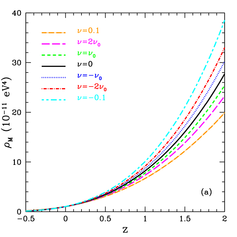
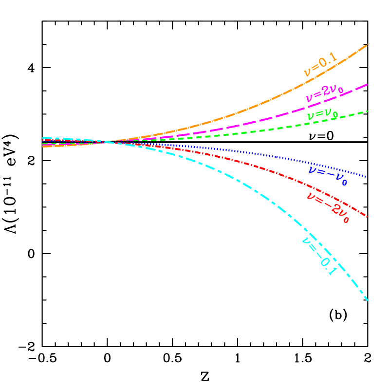
Figure 1: (a),(b) Future and past evolution of the matter density $\rho_{M}(z;\nu)$ and the cosmological constant $\Lambda(z;\nu)$ for a flat universe ($k=0$) and for different values of the fundamental parameter $\nu$ of our model ($\nu_{0}$ is defined in Eq.(59)). In both cases $\Omega_{M}^{0}=0.3$ and $\Omega_{\Lambda}^{0}=0.7$. The solid line represents the standard model case ($\Lambda={\rm const.}$), whereas the various kinds of dots/dashes represent different amounts of evolution of $\Lambda$.

In the phenomenologically most interesting case $\,|\nu|<1\,$ (see Section 4.2) we always have a null density of matter and a finite (positive) CC in the long term future, while for the far past yields $\,\Lambda=\pm\infty\,$ depending on the sign of $\,\nu$. In all these situations the matter density safely tends to $\,+\infty$. One may worry whether having infinitely large CC and matter density in the past may pose a problem to structure formation. From Fig. 1a,b it is clear that there should not be a problem at all since in our model the CC remains always smaller than the matter density in the far past, and in the radiation epoch $z>1000$ we reach the safe limit (58). Actually the time where $\Lambda(z;\nu)$ and $\rho_{M}(z;\nu)$ become similar is very recent. Take, for example, the flat case and assume the usual values of the cosmological parameters as in Fig.  1: then for $\nu=(-2\nu_{0},-\nu_{0},\,0\,,+\nu_{0},+2\nu_{0})$ equality of CC and matter density takes place at $z=(0.29,0.31,0.32,0.34,0.36)$ respectively. For larger values of $\nu$ (still in the $|\nu|\ll 1$ range), say $\nu=(-0.1,+0.1)$, we find $z=(0.27,0.43)$. In all cases the equality of matter density and CC corresponds to very recent times, and so the evolution of the CC in this model never prevented structure formation.

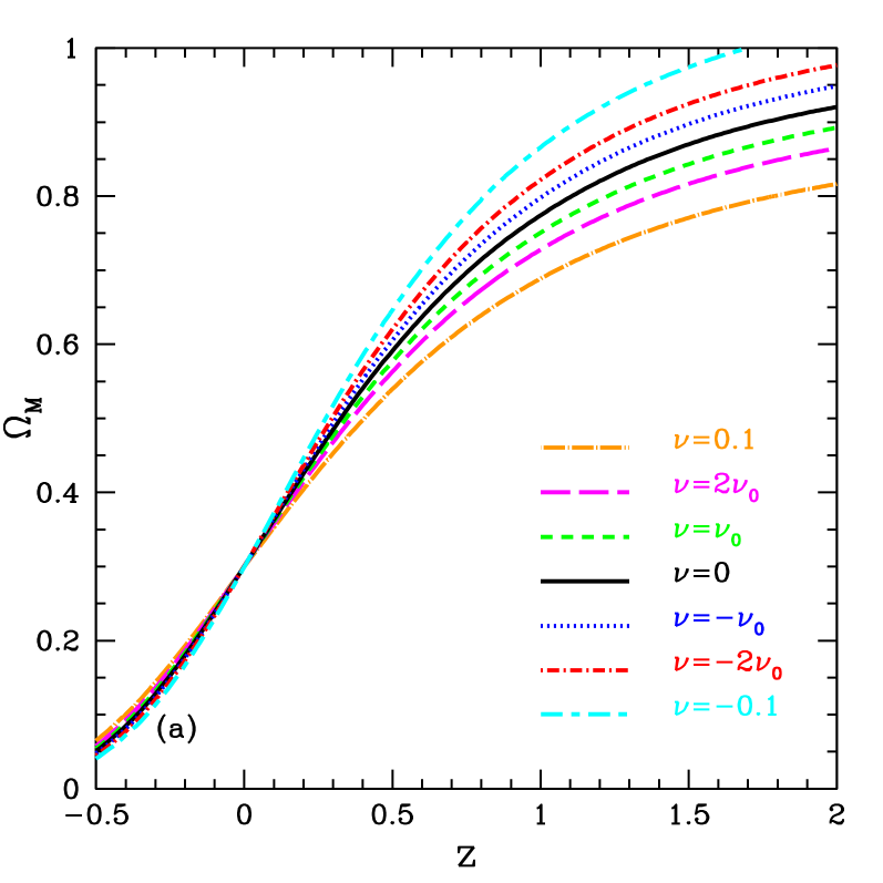
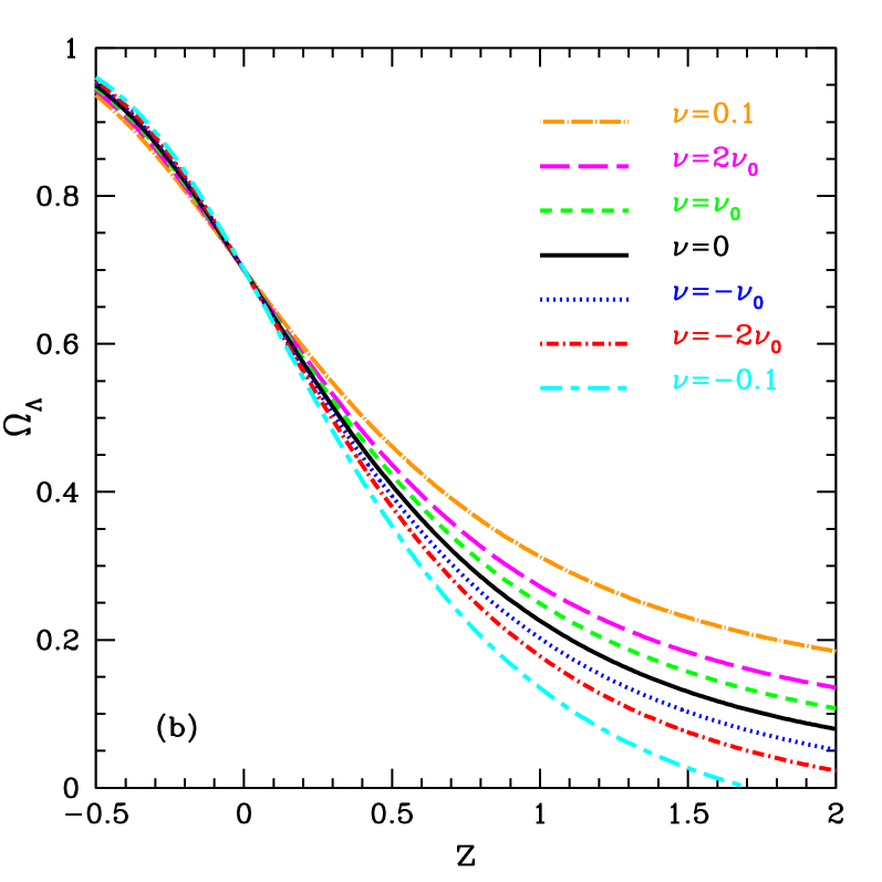
Figure 2: $\Omega_{M}(z;\nu)$ and $\Omega_{\Lambda}(z;\nu)$ versus redshift for a flat universe and different values of the parameter $\nu$, with $\Omega_{M}^{0}$ and $\Omega_{\Lambda}^{0}$ as in Fig. 1.

Related to the evolution of $\rho_{M}(z;\nu)$ and $\Lambda(z;\nu)$ are the cosmological parameters $\Omega_{M}(z;\nu)$ and $\Omega_{\Lambda}(z;\nu)$ respectively – see Fig. 2a,b. They are sensitive to the evolution of the corresponding energy densities and at the same time to that of the Hubble expansion rate $H(z;\nu)$ – see Eq. (39). The evolution of $\Omega_{M}(z;\nu)$ and $\Omega_{\Lambda}(z;\nu)$ tells us how the present values $\Omega_{M}^{0}$ and $\Omega_{\Lambda}^{0}$ differ from the corresponding values in the past and in the future for the standard model case ($\nu=0$) and the present model case ($\nu\neq 0$). Although $\Omega_{\Lambda}$ is found to be at present of the order of $70\%$ of the matter/energy in the universe, as we approach $z\sim 1$ its contribution was only a quarter of the total. The exact value obviously depends on the value of $\nu$ (Fig. 2b), being already $\sim 10\%$ larger/smaller than for a constant $\Lambda$ for $\nu=\pm\nu_{0}$ at redshift $z=1$. If we go further back in time, $\Omega_{\Lambda}(z\rightarrow+\infty)$ always diminishes, and tends asymptotically to $\nu$, while in the standard case $\,\Omega_{\Lambda}(z\rightarrow\infty)=0$. Just the opposite occurs for $\Omega_{M}(z;\nu)$ (Fig. 2a), since we are showing the flat case and so the sum has to be 1.

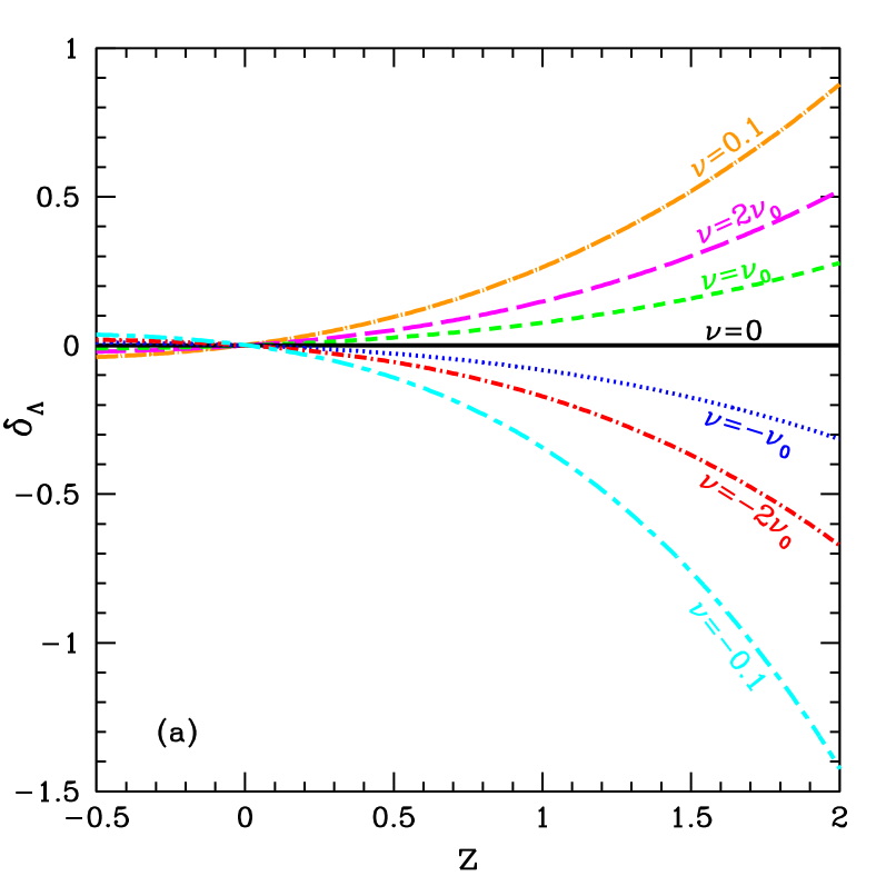
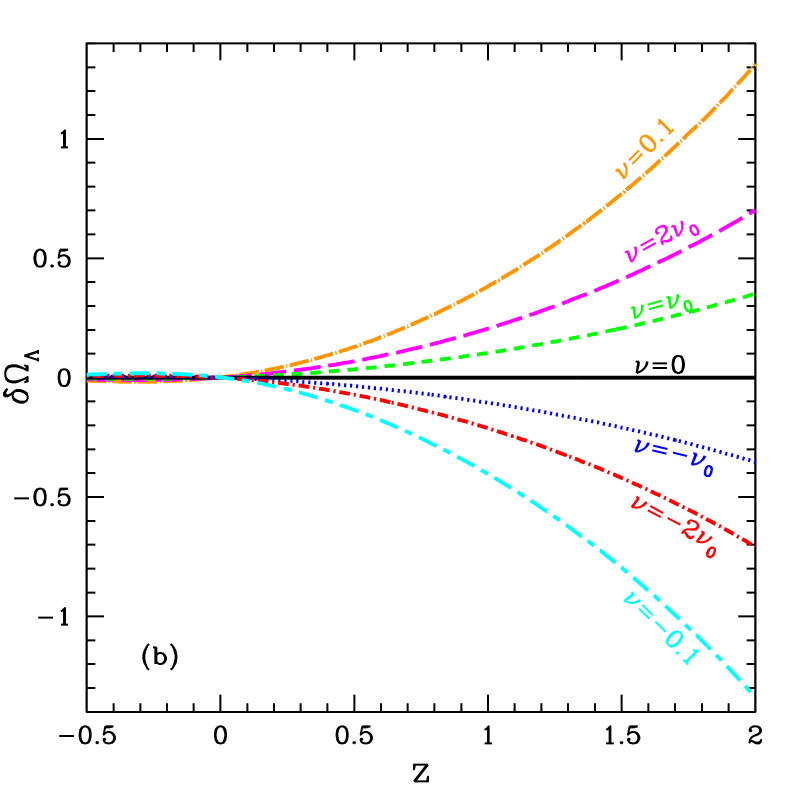
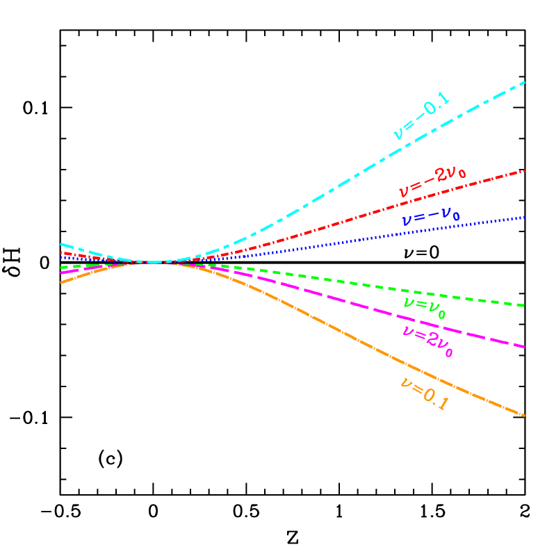
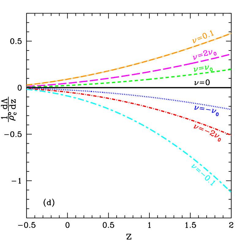
Figure 3: (a),(b),(c) Relative deviations of $\Lambda(z;\nu)$, $\Omega_{\Lambda}(z;\nu)$ and $H(z;\nu)$ from the standard $CC$ model ($\nu=0$) versus redshift for different values of $\nu$; (d) Rate of change of $\Lambda(z;\nu)$ (normalized to the present critical density) with redshift and for various $\nu^{\prime}s$. In all cases we consider a flat universe with the same parameters as in the previous figures.

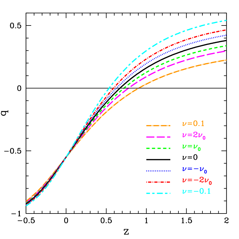
Figure 4: Evolution of the deceleration parameter, $q$, for a flat universe ($k=0$) with $\Omega_{M}^{0}=0.3$ and $\Omega_{\Lambda}^{0}=0.7$. We see that the transition from a decelerated ($q>0$) to an accelerated ($q<0$) universe takes place earlier in time (larger redshifts) for larger $\nu>0$ (see text for the exact values).

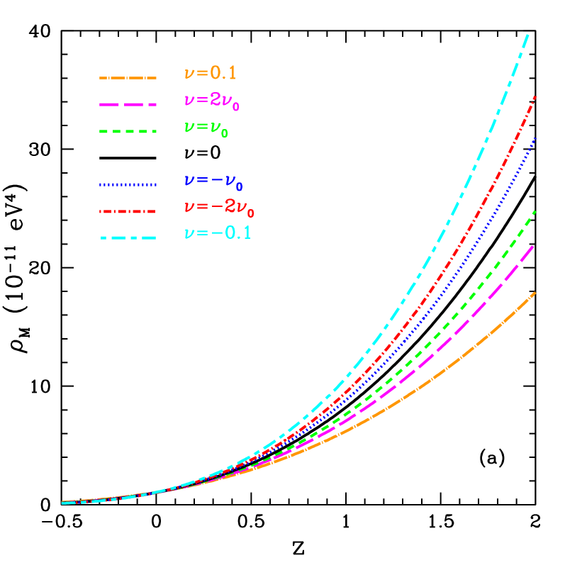
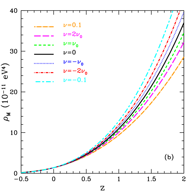
Figure 5: Evolution of the matter density for an open universe with $\Omega_{M}^{0}=0.3$ and $\Omega_{\Lambda}^{0}=0.5$ (left) and for a closed universe with $\Omega_{M}^{0}=0.4$ and $\Omega_{\Lambda}^{0}=0.8$ (right). Differences in the curves are more dependent on the value of $\Omega_{M}^{0}$ than on the curvature.

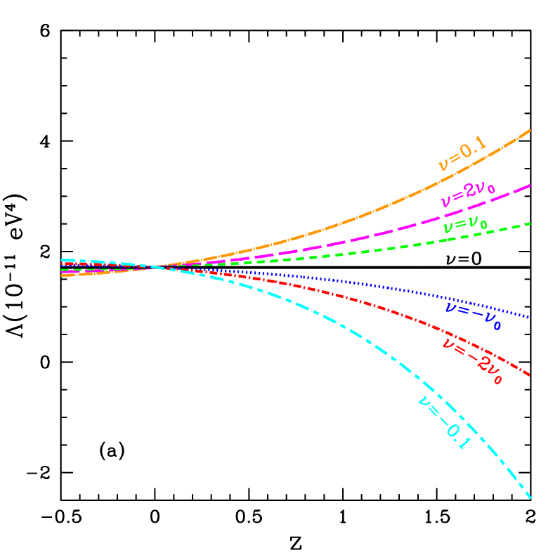
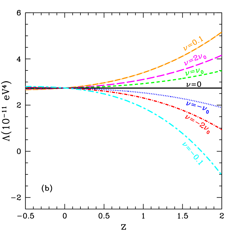
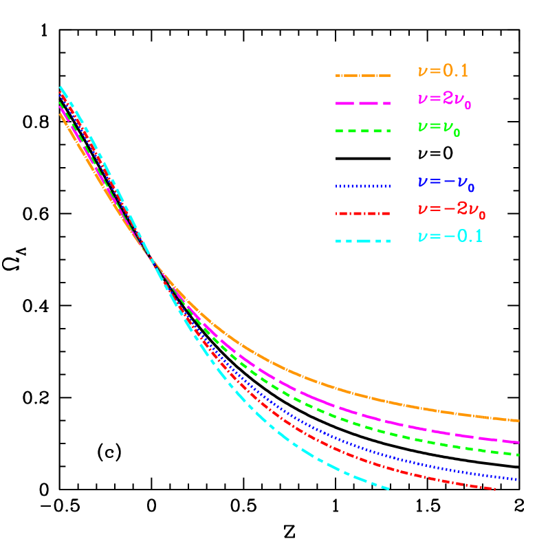
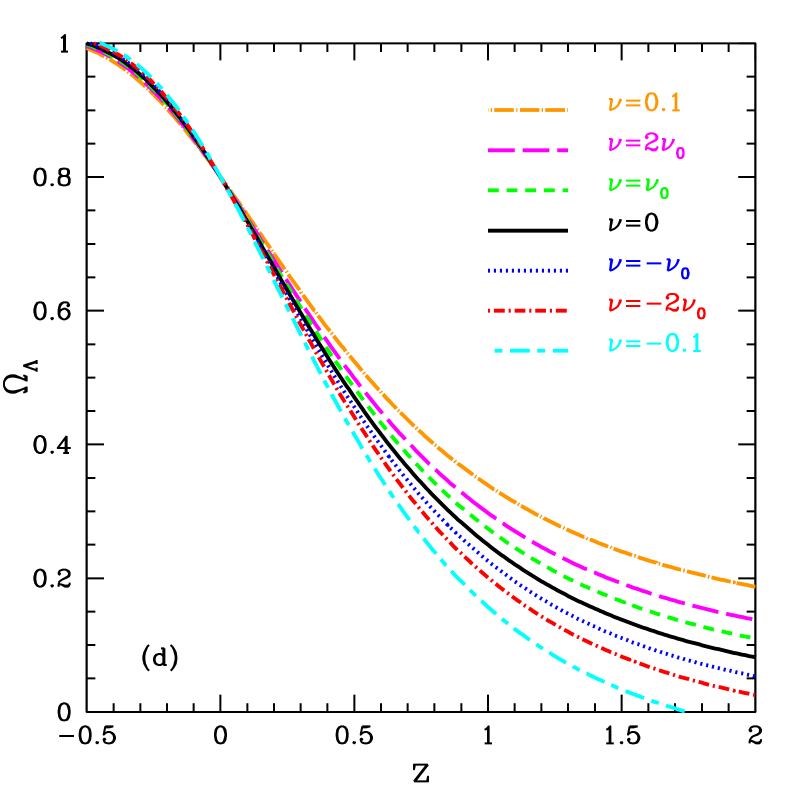
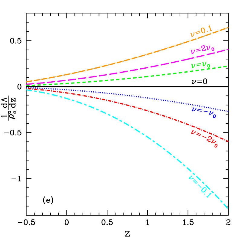
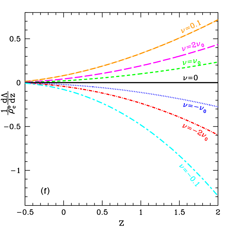
Figure 6: Cosmological constant (top), density of cosmological constant (middle) and derivative (bottom) evolutions for an open ($k<0$) universe with $\Omega_{M}^{0}=0.3$ and $\Omega_{\Lambda}^{0}=0.5$ (left) and for a closed ($k>0$) universe with $\Omega_{M}^{0}=0.4$ and $\Omega_{\Lambda}^{0}=0.8$ (right). Numerical changes with respect to the flat case are see to be most pronounced for the closed case.

In Fig. 3a,b,c we show the three deviations of the parameters $\delta\Lambda$, $\delta\Omega_{\Lambda}$ and $\delta H$ with respect to the standard model case ($\nu=0$), as defined in Section 4.2, 4.5 and 4.3 respectively. Consider first the deviation of $\,\Lambda(z;\nu)$ caused by the running. As a function of $\,z\,$ and $\,\nu$, $\,\Lambda(z;\nu)\,$ is very sensitive to $\,\nu\,$ at large $\,z$. Thus at $\,z\sim 2\,$ the increment of $\,\Lambda$ is of $50\%$ for $\,\nu=2\nu_{0}$, and once again the effect is higher for negative $\nu$ (Fig. 3a). Similar or even larger numbers are obtained for $\delta\Omega_{\Lambda}$, which attains e.g. $70\%$ under the same conditions. In contrast, the deviations $\delta H$ of the Hubble parameter from the standard value are much smaller (Fig. 3c), around $6\%$. Finally, the CC variation rate with redshift (normalized to the current critical density), $(1/\rho_{c}^{0})\,d\Lambda/dz$, is presented in Fig. 3d. These curves are non-symmetric in the sign of $\nu$ when $z$ becomes large. The effect is more important for negative $\nu$. As one can already see from $\Lambda(z;\nu)$, Eq. (35), as we go further in redshift the running increases more quickly for $\nu<0$ than for $\nu>0$.

To conclude the analysis of the flat case we consider another relevant exponent describing how the universe evolves, the deceleration parameter q. This one is fully sensitive to the kind of high-z SNe Ia data under consideration. The $\,\nu$-dependence of this parameter was discussed in detail in Section 4.6. The transition point between accelerated and decelerated expansion is a function of $\,\nu\,$: the more negative is $\,\nu$, the more delayed is the transition (closer to our time)– see Fig. 4. If $\,\nu>0$, the transition occurs earlier (i.e. at larger $z$). While in the standard case, and for a flat universe, the transition takes place at redshift 0.67 –Eq. (87) –, it would have occurred at $z=0.72$ and $z=0.78$ for $\nu=\nu_{0}$ and $\nu=2\nu_{0}$ respectively, and at $z=0.63$ and $z=0.59$ for $\nu=-\nu_{0}$ and $\nu=-2\nu_{0}$ (Cf. Fig. 4). For $\nu=(-0.1,+0.1)$ the effect is quite large, namely the transition would be at $z=(0.53,0.91)$ and hence there is a correction of $(-21\%,+36\%)$ with respect to the standard case.

5.2 Curved universe

For the small values of $\,\nu\,$ that we present in the previous figures, the differences between a flat $\,k=0\,$ universe and a $\,k=\pm 1\,$ one are not evident. A trivial variation is that coming from the different choice of the present-day values of $\,\Omega_{M}^{0}\,$ and $\,\Omega_{\Lambda}^{0}$. Besides, we have more marked $\nu$–dependent features than in a flat universe, but the main characteristics remain the same. In order to see the differences for the curved case, we show in Figures 5 and 6 the most representative parameters: $\,\rho_{M},\,\Lambda,\,\Omega_{\Lambda}\,$ and $\,{d\Lambda}/{dz}\,$, both for positive and negative curvature. Qualitatively, the behaviours are similar to the flat case. However we note that it is for positive curvature, i.e. closed universe, that we find the most dramatic numerical differences with respect to the flat case for each value of the cosmological index $\nu$. In particular, for closed universes we observe a faster running of the CC, especially for $\nu<0$ (this fact is confirmed when adopting other sets of cosmological parameters for closed universes). Therefore, $k=+1$ universes would represent the most favored case for the possibility of the observational detection of the CC running in our model. On the other hand the open universes differ numerically very slightly from the flat case even though the degree of (positive or negative) curvature chosen in the two examples shown in Figures 5 and 6 is the same, namely $\Omega_{K}=\pm 0.2$. As already advertised, from the point of view of the CMB data the curved cases under consideration would be excluded because $\Omega_{0}=1.02\pm 0.02$ [5]. However, we should still be open minded to the possibility of non-flat universes and maintain full independence of the two sets of data, CMB and high redshift SN Ia. Although we do not display the behavior of the quantities presented in the previous section due to their similarities, it might be interesting to comment where the transition from deceleration to acceleration takes place. In the case of the open and closed universes defined above the transition redshifts for $\nu=(-0.1-\nu_{0},-2\nu_{0},0,\nu_{0},2\nu_{0},0.1)$ read: $z=(0.36,0.42,0.45,0.49,0.55,0.61,0.77)$ for open, and $z=(0.49,0.53,0.56,0.59,0.62,0.65,0.73)$ for closed. So, the width of the redshift interval is almost the same as for the flat universe, but the transitions tend to occur at lower (higher) redshifts for open (closed) universes.

6 Magnitude-redshift relation and Type Ia Supernovae

The analysis of supernova magnitudes allows to test different cosmological models since magnitude depends on the dynamical evolution of the universe. This is true not only for supernovae but for all standard candles, i.e., objects whose absolute magnitude $M$ (or intrinsic luminosity ${\cal{L}}$) we know, and whose apparent magnitude $m$ (or received flux ${\cal{F}}$) can be measured at a given redshift. For cosmological purposes related to the expansion history of the universe, SNe Ia are the best candles since their luminosity enables detection up to very high redshift. Besides, although there are no standard candles in nature, in the SNe Ia case the variety is well accounted for by a tight correlation between magnitude at maximum and decline of the light curve [2, 36], and the candle can be calibrated through such correlation. A way to parameterize this effect is through the stretch factor, s, used by the Supernova Cosmology Project (SCP) [2]. The stretch factor method expands or contracts by a factor $s$ the time axis of every supernova light curve to fit a fiducial one. The stretch–corrected SNe Ia magnitudes of the sample are then fitted to obtain the cosmological parameters.

The apparent magnitude obtained at different redshifts is related to a given cosmological model via the magnitude-redshift relation. One starts from the notion of luminosity distance, $d_{L}$, related to the received flux ${\cal{F}}$ and the absolute (intrinsic) luminosity ${\cal{L}}$ through the geometric definition [1]:

$${\cal{F}}=\frac{{\cal{L}}}{4\pi d_{L}^{2}}\,.$$ (89)

Then the logarithmic relation between flux and (theoretical) apparent magnitude reads

$$m^{th}(z,H_{0},\Omega_{M}^{0},\Omega_{\Lambda}^{0})\,=\,{\cal{M}}\,+\,5\log_{10}\left[H_{0}\,d_{L}(z,H_{0},\Omega_{M}^{0},\Omega_{\Lambda}^{0})\right]\,.$$ (90)

In the last equation, terms have been defined in order to collect all the dependence on the current value of the Hubble parameter $H_{0}$ into the expression

$${\cal{M}}=M-5\log_{10}H_{0}\,+\,25\,.$$ (91)

This way all the model dependence is encoded in the luminosity-distance function $d_{L}=d_{L}(z,H_{0},\Omega_{M}^{0},\Omega_{\Lambda}^{0})$. Notice that the combined expression $H_{0}\,d_{L}$ entering the argument of the log on the r.h.s. of Eq. (90) is Hubble constant-free. On the other hand, from the FLRW metric (8), the luminosity distance of a source at (dimensionless) radial coordinate $r$ and redshift $z$ is given by $d_{L}=a_{0}\,\,(1+z)\,r$, where $a_{0}=a(t_{0})$. So we need to compute $r$ as a function of the cosmological parameters. Since our FLRW universes have been modified by the renormalization group effects represented by the $\nu$-parameter, the luminosity-distance relation takes a slightly different form as compared to the standard one [1]. This can be foreseen from the generalized structure of the $\nu$-dependent expansion rate (39) or, equivalently, the $\nu$-dependent cosmological constant parameters (68). It means that in our modified FLRW model the luminosity distance becomes a function of $\,z\,$ parameterized by $\,\nu\,$ and the present day values of the cosmological parameters: $\,\,d_{L}=d_{L}(z,H_{0},\Omega_{M}^{0},\Omega_{\Lambda}^{0};\,\nu)$. For $\nu=0$ this function reproduces the standard result. The explicit derivation of this function for $\nu\neq 0$ follows steps similar to the conventional case, namely one starts considering the equation $a\,dr=dt\,\sqrt{1-k\,r^{2}}$ for a null geodesic along a radial direction, which follows from the FLRW metric (8). This can be rewritten as

$$\frac{dr}{\sqrt{1-k\,r^{2}}}=\frac{1+z}{a_{0}}\,dt=-\frac{1}{a_{0}}\,\frac{dz}{H(z)}\,,$$ (92)

where $H(z)$ is the expansion rate at redshift $z$. Upon integration on both sides we have

$$\int_{0}^{r}\,\frac{dr^{\prime}}{\sqrt{1-k\,{r^{\prime}}^{2}}}=\frac{1}{a_{0}}\,\int_{0}^{z}\,\frac{dz^{\prime}}{H(z^{\prime},\Omega_{M}^{0},\Omega_{\Lambda}^{0};\nu)}\,,$$ (93)

where we have taken into account that in our case the expansion rate $H(z,\Omega_{M}^{0},\Omega_{\Lambda}^{0};\nu)$ is the $\nu$-dependent function $H(z;\nu)$ given by Eq. (39). After trivial integration of the l.h.s. of Eq. (93) for $k=0,\,\pm 1$ one finds the desired radial function $r=r(z,k,H_{0},\Omega_{M}^{0}\,\Omega_{\Lambda}^{0})$. Trading the curvature parameter $k$ for $\Omega_{K}^{0}=-k/H_{0}^{2}\,a_{0}^{2}$, one immediately finds the exact luminosity-distance function

$$d_{L}(z,H_{0},\Omega_{M}^{0},\Omega_{\Lambda}^{0};\nu)=\frac{1+z}{H_{0}\sqrt{|\Omega_{K}^{0}|}}\ \Psi\left(\sqrt{|\Omega_{K}^{0}|}\int_{0}^{z}{\frac{H_{0}~{}dz^{\prime}}{H(z^{\prime},\Omega_{M}^{0},\Omega_{\Lambda}^{0};\nu)}}\right)\,,$$ (94)

with

$$\Psi(x)=\left\{\begin{array}[]{lr}\sin{x},~{}~{}~{}\Omega_{K}^{0}<0\\ x,~{}~{}~{}~{}~{}~{}~{}~{}\Omega_{K}^{0}=0\\ \sinh{x},~{}~{}\Omega_{K}^{0}>0\,.\end{array}\right.$$ (95)

Here the difference with respect to the constant CC case is encoded in $H(z,\Omega_{M}^{0},\Omega_{\Lambda}^{0};\nu)$. For $\nu=0$, $H(z,\Omega_{M}^{0},\Omega_{\Lambda}^{0};\nu=0)$ becomes the standard FLRW function (40), and the luminosity distance (94) also reduces to the standard form.

We use the magnitude data from the SCP (Supernova Cosmology Project) [2]. The set includes 16 low-redshift supernovae from the Calán/Tololo survey and 38 high-redshift supernovae (Fig.7) used in the main fit of [2]. Observational data are corrected such that they can be used as the intrinsic magnitude of the object. The effective value of the magnitude is obtained from that at the peak of the light curve according to the expression:

$$m_{B}^{eff}=m_{X}^{peak}+\alpha(s-1)-K_{BX}-A_{X}\equiv m^{eff}+\alpha(s-1)\,.$$ (96)

Here $\alpha$ is the parameter describing the correlation between maximum brightness and rate of decline of SNe Ia; $s$ is the stretch factor mentioned above; X is the observed band; $K_{BX}$ is the correction to the change from the emitted B-band to the received X-band, and $A_{X}$ is the galactic extinction.

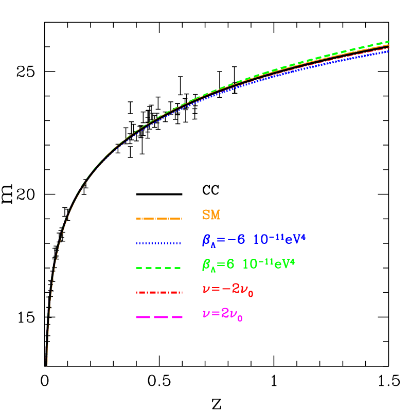
Figure 7: The magnitude-redshift relation is similar for small variations of the cosmological constant in different RG models in the literature, e.g. models with very light neutrinos and scalar fiels that could change the sign of the $\beta_{\Lambda}$ function [23, 22], or the opposite case involving the heavy fields of the SM [29]. Also shown is the standard CC case and the present model for $\nu=\pm 2\nu_{0}$. Points represent the 54 SNe used in the main fit from [2]

Figure 7 represents, in the magnitude-redshift space, the data obtained by the SCP Collaboration together with the predicted magnitude-redshift relation for our model based on the scale (16) and two RG models based on the scale (14) [23, 29]. At low redshift all the models are equivalent as it occurs with all the alternative models to the standard one. At high redshift they display small variations with respect to the “constant CC” cosmological model. As it is seen graphically, current data are not able to distinguish between models. At present, this kind of models can only be favored theoretically (see Section 7 for the future prospects).

In order to determine the cosmological parameters we use a $\chi^{2}$-statistic test, where $\chi^{2}$ is defined by the difference between the theoretical apparent magnitude and the observed one:

$$\chi^{2}(\Omega_{M},\Omega_{\Lambda},\nu,\alpha,{\cal{M}})=\sum_{i}\frac{\left\{{\cal{M}}+5\log_{10}\left(H_{0}\,d_{L}(z_{i},H_{0},\Omega_{M},\Omega_{\Lambda},\nu)\right)-m_{i}^{eff}-\alpha(s_{i}-1)\right\}^{2}}{\sigma_{i}^{2}}$$ (97)

As we are only interested in the cosmological parameters associated to the acceleration of the universe, we marginalize over $\alpha$ and ${\cal{M}}$ [2, 54]. That means that we minimize $\chi^{2}$ by integrating over all possible values of $\alpha$ and ${\cal{M}}$.

6.1 Results from current data

In this section, confidence levels surrounding best fits (minimum $\chi^{2}$) are given by contour lines of constant $\chi^{2}$, which represent $1\sigma$, $2\sigma$ and $3\sigma$ confidence levels respectively.

A distinguishing feature of all the models is the evolution of the cosmological constant, thus we can make a first test in order to see whether such an evolution is consistent with current data. We adopt a generic form for the Hubble parameter which describes any CC running:

$$H^{2}(z)=H_{0}^{2}\,\left[\Omega_{M}^{0}\,(1+z)^{3}+\Omega_{\Lambda}^{0}+\frac{1}{\rho_{c}^{0}}\left.\frac{d\Lambda}{dz}\right|_{z=0}\,z+\Omega_{K}^{0}\,(1+z)^{2}\right]\,.$$ (98)

This equation parameterizes generically the deviations from the standard law (40) through a series expansion of $\Lambda(z)$ up to first order in $z$, or equivalently up to the term defining the $\beta$-function for each model - remember that $d\Lambda/dz=\beta_{\Lambda}\,d\ln H/dz$. We may therefore distinguish models by plugging in the corresponding $\beta$-function in this formula.

In Fig. 8a the confidence region in the $(\Omega_{\Lambda}^{0},({1}/{\rho_{c}^{0}}){d\Lambda}/{dz}\left|{}_{z=0}\right.)$ space for a flat universe is shown. It does by no means discard the running of the cosmological constant. In some sense this is similar to what happens with quintessence models where data are compatible with a slow evolution of a scalar field, but here we are testing the evolution of a density component without any variation in the equation of state. When we restrict ourselves to the constant cosmological term, $d\Lambda/{dz}=0$, we recover results similar to the standard ones, namely $\Omega_{M}^{0}\sim 0.3\pm 0.1,\Omega_{\Lambda}^{0}\sim 0.7\pm 0.1$ for a flat geometry (Cf. Fig. 8a). In this case the minimum $\chi^{2}$ value lies at $\Omega_{M}^{0}=0.29,\Omega_{\Lambda}^{0}=0.71$. But in general we see from Fig.  8a that this commonly accepted value may undergo a wide variation when the possible running of the cosmological constant is taken into account.

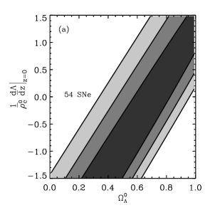
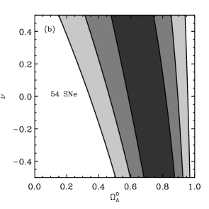
Figure 8: (a) Confidence regions for the current cosmological constant density and its variation with redshift for a flat universe– Cf. Eq. (98). From darkest to lightest the regions correspond to $1\sigma$, $2\sigma$ and $3\sigma$ respectively. A running CC clearly provides a wider interval of possible values for $\Omega_{\Lambda}^{0}$ with the same probability; (b) Confidence regions for $\Omega_{\Lambda}^{0}$ and the representative parameter $\nu$ of our model with running CC.

After this generic observation, we turn to our model and apply a $\chi^{2}$ test to obtain confidence regions in the $(\Omega_{\Lambda}^{0},\nu)$-plane for a flat universe (Fig. 8b). We see there that $\Omega_{\Lambda}^{0}$ does not vary significantly with different values of $\nu$. This is because the sample of supernovae used has redshift up to $0.83$ (Cf. Fig. 7) and the average is $z\sim 0.5$. However, as it was already observed in Fig. 1, the effect becomes more important as we go to higher $z$, and we will thus be able to draw more trustworthy conclusions when we analyze SNAP data, which will reach up to $z=1.7$.

7 SNAP and the running cosmological constant

After the discovery of the accelerated expansion of the universe [2, 3] a new satellite observatory (SuperNova Acceleration Probe) was proposed to determine the nature of the dark energy cause of the acceleration. The SNAP collaboration aims to obtain spectra and photometry for 2,000 supernovae already in the first year of mission [34]. The distribution of supernovae will have a maximum in the interval $0.2<z<1.2$ where according to the present observed rates 1800 supernovae should be found. A smaller number of data is expected to be obtained up to a redshift of 1.7 (see more details in [34]).

We suppose that supernovae are equidistant within every redshift interval, and obtain the magnitude for these supernovae within the cosmological model presented in this work. In each case observational gaussian errors are added to these values taking into account the systematic uncertainties, which are estimated to be zero at z=0 and 0.02 at z=1.5 following, for instance [55]: $\sigma_{sys}=~{}z~{}({0.02}/{1.5})$ and the intrinsic dispersion of supernovae after the corresponding calibrations $\sigma_{intr}=~{}0.15$.

After fitting the models to their simulated data we have an idea of the precision with which we will determine the parameters and the possibility of distinguishing among models. Moreover, when the first results of SNAP will become available, the value of $\Omega_{M}^{0}$ should already be known to a high precision. We can therefore adapt the present study to this foreseeable situation and use a Bayesian analysis in order to determine the probability of our parameters given some prior information. Details of the statistical methods used are shown in Appendix 2.

7.1 High–z samples and the determination of $\nu$

With the SNAP sample we will have, at high redshift, groups of 20 supernovae per bin of width 0.01 in redshift. This means that the uncertainty in the magnitude at each bin will be of the order of only 0.03 magnitudes for the present intrinsic dispersion of 0.15 magnitudes.

We can take one of this bins at relatively low redshift ($z_{1}=0.5$) and another one at higher redshift ($z_{2}=1.0\,$ or $\,1.5$) to look at the intersection between the allowed regions in the parameter space (Fig. 9). This intersection represents how the intrinsic dispersion in magnitude translates into the parameters according to ($\Delta\Omega_{\Lambda}\times\Delta\Omega_{M})\propto(\sigma_{m}^{z_{1}}\times\sigma_{m}^{z_{2}})$ (see for instance [56]).

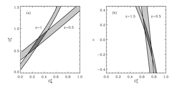
Figure 9: Bands of constant magnitude in the parameter space, where magnitudes are obtained for a universe with $\Omega_{M}^{0}=0.3,\Omega_{\Lambda}^{0}=0.7,\nu=2\nu_{0}$. The plot on the left shows the intersection between the bands coming from two supernovae at $z=0.5$ and $z=1.0$ on the ($\Omega_{M}^{0},\Omega_{\Lambda}^{0}$)-plane. On the right the plot is on the ($\Omega_{\Lambda}^{0},\nu)$-plane where the two supernovae need to be more distant in redshift in order to equally restrict the confidence region.

Figure 9 shows the results when the running of the cosmological constant is considered. In the left panel the bands of constant magnitude are plotted in the usual space of cosmological parameters. The cosmological model used is one with $\Omega_{M}^{0}=0.3,\Omega_{\Lambda}^{0}=0.7,\nu=2\nu_{0}$ and the bands give a similar intersection as in a standard model with $\Omega_{M}^{0}=0.3,\Omega_{\Lambda}^{0}=0.7$ (Fig. 2 in [56]), so the present-day parameters will be determined under the same conditions in both kinds of models. But we can also see how the cosmological index is determined by the SNAP measurements. In order to obtain a reduced confidence region in the ($\Omega_{\Lambda}^{0},\nu$) plane, we need data more separated in redshift than in the previous case. This is because the interesting models with standard (non-variable) cosmological constant have their maximum difference at $z\sim 0.8$ (this value is that obtained for the difference between a $\Omega_{M}^{0}=0.3,\Omega_{\Lambda}^{0}=0.7$ universe and a $\Omega_{M}^{0}=0.2,\Omega_{\Lambda}^{0}=0$ universe). Models with a running cosmological constant differ from the ones without such running CC at higher redshift ($z>1$) and the difference grows with $z$. Thus, as we see in Fig. 10, we need a sizeable group of supernovae at the highest redshift reachable by SNAP while a strong concentration of data around $z=1$ is needed to distinguish models with and without cosmological constant.

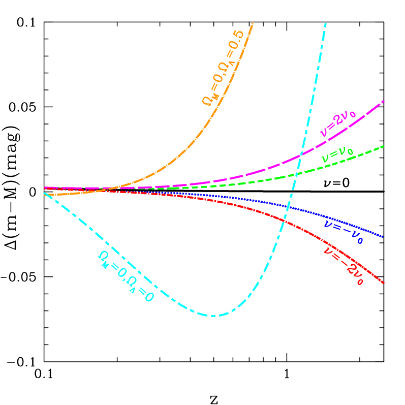
Figure 10: Deviations of the distance modulus $m-M$ with respect to the case of a standard cosmological constant with $\Omega_{M}^{0}=0.3,\Omega_{\Lambda}^{0}=0.7$ or equivalently $\nu=0$. Two fully academic situations are shown: $(\Omega_{M}^{0},\Omega_{\Lambda}^{0})=(0,0)$ –Milne’s open universe– and a pure de Sitter’s universe $(0,0.5)$, both with no matter, in order to show the scope of the effects. Important differences appear for $z\gtrsim 0.5$. The other curves in the graphic show the case of the more realistic model presented in the paper, for various values of $\nu$. Differences become important at $z\gtrsim 1$.

7.2 Numerical simulations for SNAP and other high–z SNe Ia samples

We now use the distribution of data predicted by the SNAP collaboration and some alternative distributions to obtain the confidence regions for the representative parameter of the model, $\nu$. However, as we have done with the current data, we first use the distinctive characteristic of the variable CC models, namely the presence of a term ${d\Lambda}/{dz}$ different from zero. The order of magnitude of these derivatives in our model model can be directly read from Fig.  3d. At the present epoch $({1}/{\rho_{c}^{0}}){d\Lambda}/{dz}=3\nu\Omega_{M}^{0}\sim 0.05$ for $\nu=2\nu_{0}$. As seen in the figures, Eq. (98) is not a sufficiently good approximation in this case since the Taylor expansion is only significant at first order. Therefore, in our model we would have to use the second derivative as well in order to study the change of slope at high redshift. The other parameters used in the simulation are a flat universe with $\Omega_{M}^{0}=0.3,\Omega_{\Lambda}^{0}=0.7$.

For such a universe we obtain, after the SNAP project, the results in Fig. 11. The left panel shows the confidence regions in the ($\Omega_{\Lambda}^{0},({1}/{\rho_{c}^{0}}){d\Lambda}/{dz}\left|{}_{z=0}\right.$) plane when a flat universe is considered, and the right panel adds a gaussian prior on $\Omega_{M}^{0}$ with $\sigma_{\Omega_{M}}=0.03$. These restrictions in the analysis are justified by recent results of the WMAP experiment [5]. Thus, with all these considerations, $({1}/{\rho_{c}^{0}}){d\Lambda}/{dz}$ at the present epoch would be obtained to within $\pm 0.2$ which could distinguish models like the one presented here from the standard cosmological constant model.

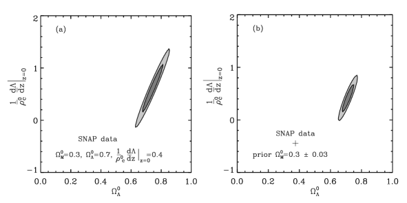
Figure 11: Confidence regions in the ($\Omega_{\Lambda}^{0},({1}/{\rho_{c}^{0}}){d\Lambda}/{dz}\left|{}_{z=0}\right.$) plane for a flat universe. The left (right) plot has been obtained without (with) restriction (i.e. prior) in the knowledge of $\Omega_{M}^{0}$. Data used in the fits are those obtained with the SNAP distribution of 2,000 supernovae as explained in Section 7.

The results for the parameter $\nu$ are shown in Fig. 12. Fits are made under the same assumptions as in the previous case and so the results represent the expected accuracy in the parameters using all the information to come. Thus we determine $\nu$ to $\pm 0.06$ for $\nu=0.1$. We must take into account, however, that the SNAP distribution of data is optimized in order to distinguish models that have their maximum difference at a redshift near 1. We can, therefore, try other distributions designed from the idea that the difference between models grows with redshift, as it indeed happens in our case. The first distribution is very similar to the SNAP one but with most of the data homogeneously distributed between $z=0.2$ and $z=1.7$. This second distribution extends data up to redshift $z=2$. This is in part justified by data which are being obtained within the GOODS and HST Treasury Program [35].

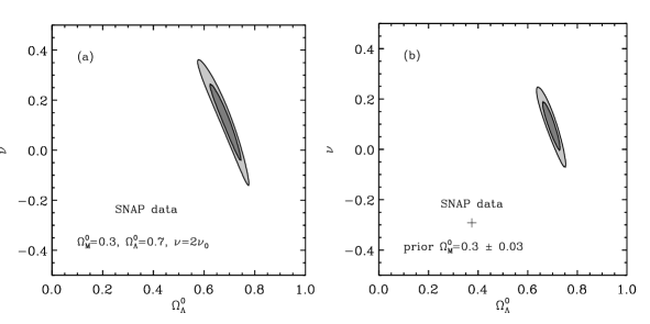
Figure 12: $1\sigma$ and $2\sigma$ confidence regions for the basic parameter $\nu$ of our model and the current value of $\Omega_{\Lambda}$. Left panels shows the results with SNAP data in a flat universe whereas right panels add a restriction (prior) on $\Omega_{M}^{0}=0.30\pm 0.03$. The distinction is only made at $1\sigma$ level within the range of $\nu$ with physical meaning.

The results from the various distributions are shown in Fig. 13 and quantified in Table 1. The latter also compares the determination of the parameters representing an RG evolution of the cosmological constant (i.e. $\nu\neq 0$), and the evolution of the equation of state (see Eq. (11)) for an alternative dark energy model. We see that the evolution of the cosmological constant can be determined with a relative error of $60\%$ for a value of $\nu=0.1$. Distributions of data other than SNAP (Distr.1 and Distr.2 in Table 1) allow to reduce this error to $20\%$ with $\nu=0.1$, but determinations remain poor for small values of $\nu$, which on the other hand would be the natural ones. We are then in a situation similar to the determination of the evolution of the equation of state, Eq. (11). Although $w_{0}$ can be obtained with a precision of $2\%$ for $w_{0}\sim-1$, its evolution $w_{1}$ is only determined with great uncertainty. For instance, the evolution of $w$ for SUGRA described by [57] is expected to be determined with a relative error in $w_{a}\sim 2w_{1}$ of 43 $\%$. In our case, as for other dark energy candidates, very high–z samples as the ones being collected by GOODS and HST Treasury program will significantly contribute to the precise determination of $\nu$.

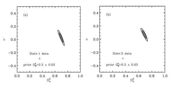
Figure 13: Confidence regions in the $(\Omega_{\Lambda}^{0},\nu)$ space with data distributions (see Table 1) alternative to the standard SNAP one. This way provides a better determination of the parameters.

Distribution	Data	Prior $\sigma_{\Omega_{M}}$	$\theta$	$\sigma_{\theta}$
SNAP	50 SNe $0<z<0.2$
(1 year)	1800 SNe $0.2<z<1.2$
	50 SNe $1.2<z<1.4$
	15 SNe $1.4<z<1.7$	None	$\nu=0.1$	$\pm 0.10$
SNAP	as above	0.03	$\nu=0.1$	$\pm 0.06$
SNAP	3 years	None	$\nu=0.1$	$\pm 0.06$
SNAP	3 years	0.03	$\nu=0.1$	$\pm 0.04$
Distr.1	50 SNe $0<z<0.2$
	2000 SNe $0.2<z<1.7$	0.03	$\nu=0.1$	$\pm 0.05$
Distr.2	250 SNe $0<z<1$
	1750 SNe $1<z<2$	0.03	$\nu=0.1$	$\pm 0.02$
SNAP	3 years	0.03	$w_{0}=-1$	$\pm 0.02$
SNAP			$w_{a}=0.58$	$\pm 0.25$

Table 1: Determination of the parameters with SNAP data and with other two distributions. In all cases the cosmology used for the analysis is a flat universe, and when a prior on $\Omega_{M}$ is added we use a central value of $\Omega_{M}=0.3$. For comparison we show the parameters representing variations in the equation of state (11) (for SUGRA in [57]).

8 Conclusions

To summarize, we have constructed a semiclassical FLRW model with variable CC at the present cosmic scale. The variation of the vacuum energy is provided without introducing special scalar (quintessence-like) fields and is completely caused by quantum effects of vacuum. The evolution of the CC is due to the Renormalization Group running triggered by the smooth decoupling of the massive fields at low energies, while the RG scale $\mu$ being associated to the Hubble parameter, $H$, at the corresponding epoch. Although the $\beta_{\Lambda}$-function itself is proportional to the fourth power of the masses, the decoupling does still introduce an inverse power suppression by the heavy masses, and thus one is left with a residual quadratic law $\beta_{\Lambda}\sim H^{2}M^{2}$. The effective scale $M$ summarizes the presence of the heaviest degrees of freedom available. This peculiar form of decoupling stems directly from:  i) the Appelquist-Carazzone (AC)-decoupling theorem,  ii) general covariance, and also from  iii) the non-fine-tuning hypothesis between the $n=1$ (“soft decoupling”) terms of $\beta_{\Lambda}$ (Cf. Eq. (12)) whereby the overall coefficient of the quadratic contribution $H^{2}M^{2}$ does not vanish. This particular form of decoupling is a specific characteristic of the CC because it is of dimension four. There is no other parameter either in the SM or in the GUT models with such property.

In constructing the cosmological model we have explored the possibility that the heaviest d.o.f. may be associated to particles having the masses just below the Planck scale. This assumption is essential to implement the soft decoupling hypothesis within the $\mu=H$ setting. Indeed, the present value of $\,H_{0}^{2}M^{2}\,$ is just of the order of the CC, and therefore it insures a smooth running of the cosmological term around the present time. In this setting the $\beta_{\Lambda}$-function has only one arbitrary parameter $\,\nu\,$ (33), and as a result the model has an essential predictive power. In general we expect $\,|\nu|\ll 1\,$ from phenomenological considerations, mainly based on the most conservative hypotheses on the nucleosynthesis framework. Furthermore, for $\,|\nu|\ll 1$, we insure the absence of the trans-Planckian energies. It is not completely clear how much the cosmological index $\,\nu\,$ can approach the value $1$ from below. Despite the values $\nu\lesssim 1$ are not completely ruled out, it is not clear that the conditions for the nucleosynthesis could be safe. However, if accepted, it opens up the possibility that the CC could be in transit from a $\,\Lambda>0\,$ regime into a future $\,\Lambda\leq 0\,$ one, which would be a welcome feature for string/M-theory.

Our RG model offers the possibility to explore the existence of the sub-Planck physics in direct cosmological experiments, such as SNAP (and the very high–z SNe Ia data to be obtained with HST). For example, for the flat FLRW case and a moderate and positive value $\nu\sim 10^{-2}$, we predict an increase of $10-20\%$ in the value of $\Omega_{\Lambda}$ at redshifts $z\gtrsim 1-1.5$ perfectly reachable by SNAP. For similar, but negative, values of $\nu$ we predict that the CC should become negative beyond redshifts $z\gtrsim 2$. For $\nu\sim 0.1$ corrections to some FLRW cosmological parameters become as large as $50\%$ or more. In general, this model has a wide spectrum of implications that could be tested by SNAP, even for fairly moderate values of $\nu$ compatible with the most conservative bounds from nucleosynthesis. The simulations of the SNAP data in Section 7 show that the single parameter $\nu$ of our model could be pinned down, for $\nu\lesssim 0.1$, with a precision of around $20-60\%$. Although this accuracy is not very high, the sign of the parameter could be determined and the effects would be manifest. Undoubtedly, this would be a good starting point to identify the presence of quantum corrections to the FLRW classical cosmology.

The semiclassical FLRW model that we have proposed here explains the variation of the CC due to the “relic” quantum effects associated to the decoupling of the heaviest degrees of freedom below the Planck scale, and suggest that a time dependence of the CC may be achieved without resorting to scalar fields mimicking the cosmological term or to modifications of the structure of the SM of the strong and electroweak interactions and/or of the gravitational interactions. At the same time, our model provides a phenomenological parametrization for possible correlated deviations of the cosmological equations for matter density and dark energy.

From a more fundamental point of view, we have shown that the cosmological constant and the matter density may evolve in a correlated way due to quantum effects without resorting to exceedingly exotic frameworks. Using the RG as a basic QFT tool and extrapolating the standard AC law of decoupling to the CC case, we have straightforwardly predicted a cubic redshift evolution law for the CC and the matter density. The larger the redshift that we can eventually explore the larger the effects that we predict. Most important, we have shown that this cubic law can be thoroughly tested by the next generation of cosmological measurements, which will be able to reach depths up to $z\sim 2$.

9 Appendix 1. On the non-local terms in the quantum corrections.

In this appendix we shall go beyond the phenomenological presentation used throughout the main text and briefly discuss some theoretical aspects of our QFT framework. Despite the cosmological model developed in the main text of the paper looks appealing due to its relative simplicity and relation to the QFT corrections, it is not immediately clear which level of credibility can be granted to the hypothesis of the “soft” low-energy decoupling which we used here. As it was already remarked in the main text, the physical interpretation of the renormalization group in curved space-time requires the formalism beyond the limits of the well-known standard techniques. These techniques are essentially based on the minimal subtraction $\,\overline{MS}\,$ scheme of renormalization [43, 44, 58, 25], which does not admit to observe the decoupling.

The physical interpretation of the renormalization group in the higher derivative sector can be achieved through the calculation of the polarization operator of gravitons arising from the matter loops in linearized gravity [46]. In this case one can perform the calculations in the physical mass-dependent renormalization scheme (specifically, in the momentum subtraction scheme, in which $\mu$ is traded for an Euclidean momentum $p$), obtain explicit expressions for the physical beta-functions and observe the decoupling of massive particles at low energies. In the mass-dependent scheme one has direct control of the functional dependence of the $\,\beta$-functions on the masses of all the fields, i.e. one knows explicitly the functions $\,\beta_{k}(m_{i};p^{2}/M^{2}_{j})\,$ for the higher derivative terms $a_{k}$ in (4). Quite reassuring is the fact that these momentum subtraction $\,\,\beta$-functions boil down, in the UV limit, to the corresponding $\,\,\beta$-functions in the MS scheme [46].

Unfortunately, as it was realized in [46], this program fails when we attempt to derive the physical $\,\beta$-function for the CC (and also for the inverse Newton constant $\,1/G$). In fact, within the momentum subtraction scheme we fail to see the $\,\beta$-function for CC and for the inverse Newton constant $\,1/G\,$ at all, so there is no correspondence with the $\,\overline{MS}\,$ scheme in these sectors. The origin of the problem is that the standard renormalization group running always corresponds to the non-local insertions in the effective action. For example, in case of QED the one-loop terms look, in the UV, like

$$\Gamma_{QED}\,=\,\int d^{4}x\,\sqrt{-g}\,\,\Big{\{}\,\,-\frac{1}{4}F_{\mu\nu}F^{\mu\nu}+\frac{e^{2}}{3(4\pi)^{2}}F_{\mu\nu}\,\log\Big{(}\frac{\square}{m_{e}^{2}}\Big{)}\,F^{\mu\nu}\,\Big{\}}\,.$$ (99)

In the $\overline{\rm MS}$-scheme of renormalization the total $\mu$-independence of the effective action (see, e.g. [25]) is provided by the running of the coupling $\,e=e(\mu)$. This running is a physical effect which has been observed experimentally [59]. As noted before, if we wish to describe low energy effects $p^{2}\ll m_{e}^{2}$, we need a more physical subtraction scheme where the role of $\mu$ is played by the momentum $p$. Then we expect decoupling terms of the form $p^{2}/m_{e}^{2}$, which manifest as additional $\square/m_{e}^{2}$ terms (without logarithms) in the effective action (99). Similarly, in the higher derivative gravitational sector we have the terms of the form

$$\Gamma_{HD}\,=\,\int d^{4}x\,\sqrt{-g}\,\,\big{\{}\,C_{\mu\nu\alpha\beta}\,k_{1}(\square,m^{2})\,C^{\mu\nu\alpha\beta}\,+\,R\,k_{2}(\square,m^{2})\,R\,\big{\}}\,,$$ (100)

where $\,C_{\mu\nu\alpha\beta}\,$ is the Weyl tensor, $\,R\,$ is a scalar curvature, $m$ is any particle mass and $\,k_{1}\,,\,k_{2}\,$ are definite non-local functions [46] which in the high energy region include $\,\ln(\square/m^{2})$. As in the QED case, at low energy these functions contain the decoupling terms $\square/m^{2}$ without logs. When the derivative operators act on the conformal factor $a(t)$, they produce terms proportional to the powers of the Hubble parameter $H$ and its derivatives. Since the derivative ${\dot{H}}$ of the Hubble parameter has the same order of magnitude as $H^{2}$, for the sake of simplicity we can consider only the powers of $H$. It is clear that the finite order non-localities can be described, at low energies, by the local expansions with the tensor structure similar to the one of (100). For instance, making the expansion in the powers of $\,\square/m^{2}$, we meet the quadratic law of the low-energy decoupling.

Let us now consider the cosmological and Einstein-Hilbert terms. In the $\overline{\rm MS}$-scheme the $\mu$-dependence of the form of the effective action is compensated by the running of the parameter $\,\Lambda$, similar to the QED case and the running $e(\mu)$. As a result the overall effective action with a running CC is scale-independent, as it has to be. We are able, in principle, to observe the CC only at very small energies, and naturally expect to have much weaker running because of the low-energy decoupling. However, the quantitative investigation of the phenomena of decoupling for the CC met very serious difficulties, starting from the physical interpretation of the renormalization group in this case. As noticed in [46], the non-local insertions can not be done in the original gravitational terms, because acting on $\Lambda$ by $\,\square\,$ we get zero and $\,\square\,$ acting on $\,R\,$ gives a total derivative. The insertion can be done only into the non-local terms with similar global scaling, e.g.

$$\int d^{4}x\sqrt{-g}\,R_{\mu\nu}\Big{(}\frac{m^{2}}{\square}\Big{)}^{2}\,R^{\mu\nu}\qquad\mbox{and}\qquad\int d^{4}x\sqrt{-g}\,R_{\mu\nu}\Big{(}\frac{m^{2}}{\square}\Big{)}R_{\mu\nu}$$ (101)

for the CC and inverse Newton constant respectively. For the effective action of the quantized massive fields these terms do not take place and hence the framework of linearized gravity is not appropriate for the physical interpretation of the renormalization group for the CC and $\,1/G\,$ in curved space. Does it mean that there is no other framework where this interpretation should appear in a natural way? From our point of view it is not really so. Let us remind that:

1.   The renormalization group for the CC and $\,1/G\,$ can be formulated in a very robust way in curved space if we use the $\,\overline{MS}$ renormalization scheme. Therefore, we can expect the coincidence with the physical RG in an appropriate framework.

2.   The linearized gravity approach is essentially based on the expansion near the flat background. But when quantizing massive fields we have to introduce the vacuum CC from the very beginning in order to provide renormalizability. In this case the flat Minkowski space-time is not a solution of the classical equations of motion and the whole approach based on the linearized gravity is formally illegal. Perhaps this is the source of the problem.

In order to see the renormalization group and decoupling for the CC and $\,1/G\,$ one has to perform calculations of the polarization operator or vertices on the non-flat dynamical background. In this case there will be no relation between the covariant expansion in curvatures and the gravitational perturbations around the given metric. From the point of view of the linearized gravity this means that we can not achieve the physical interpretation of the renormalization group via the gravitational perturbations around the flat metric background, because all the effect is essentially non-perturbative. In some sense the situation is similar to the low-energy QCD, where one has to rely on the non-perturbative methods or reformulate the perturbative calculations using, e.g. the renormalon technique. It might happen that the resummation of the perturbative series coming from both quantum loop expansion and the gravitational perturbations may lead to the visible renormalization group effect, but at present it is unclear how this could be checked.

Let us consider again the linearized gravity approach. The non-localities of the effective action of the massive fields are related to the insertions of the “massive” Green functions $\,{1}/(\square+m^{2})\,$. Then, making the expansion in the powers of $\,\square/m^{2}$, we meet, typically, much stronger decoupling than the standard quadratic one. However, since we are dealing with an infinite multiple series, the correspondence with the $\,\overline{MS}$ scheme means that some resummation of the series in curvature produces the massless $\,\,{1}/{\square}\,$ insertion which may eventually lead to the soft decoupling and to the UV correspondence with the $\,\overline{MS}$ scheme.

At present there is no method of calculations on the non-flat background compatible with the physical renormalization scheme. In this situation our phenomenological approach looks rather justified. The covariance of the effective action forbids the first order in $\,H\,$ corrections. Then, recalling that the UV contribution to $\,\beta_{\Lambda}\,$ from a particle of mass $\,m\,$ is $\beta_{\Lambda}\sim m^{4}$ – Cf. Section 3– the low-energy contributions to $\,\beta_{\Lambda}\,$ must be supressed by, at least, the factor

$$\square/m^{2}\,\,\sim\,\,H^{2}/m^{2}\,,$$ (102)

and hence the overall low-energy $\,\beta_{\Lambda}\,$ acquires the form $H^{2}\,m^{2}$, Eq. (17). The same form of decoupling can be expected for the induced counterpart $\Lambda_{ind}$ of the CC. The renormalization group equations for the vacuum and induced CC’s are independent, and the relation emerges only at the moment when we choose the initial point of the RG trajectory for the vacuum counterpart [22, 23]. In fact, the Feynman diagrams corresponding to the $\Lambda_{ind}$ are, at the cosmic scale, very similar to the vacuum ones, because the Higgs field $\phi$ is in the vacuum state, $<\phi>\neq 0$, and the non-zero contribution of these diagrams is exclusively due to the momenta coming from the graviton external lines. Finally, there is no real need to distinguish induced and vacuum CC’s in the present context. In both cases the absence of the $n=0$ order (non-supressed) contributions in (12) is required by the apparent correctness of the Einstein equations and the smallness of the observable CC. There is no guarantee that the IR supression does not take a much stronger form than the one (soft quadratic decoupling) assumed here. In the last case the future experiments and observations will demonstrate a perfectly constant CC. The same should happen if the high-energy spectrum does not include the particles with the masses comparable to $\,M_{P}$. In both these cases the effect of running would be negligible. Then, since our renormalization-group based model gives very definite prediction for many observables (see Sections 4,5), it should be, sooner or later, distinguished from the standard model with the $\,z$-independent CC or maybe even from the quintessence models.

One could wonder whether the non-local effects behind the renormalization group are compatible with the standard energy conservation equation which we used in the text. In fact, the covariant form of the conservation law $\,<\nabla_{\mu}T^{\mu}_{\nu}>=0\,$ just reflects the covariance of the effective action and therefore does not depend on the non-localities which are always present in the quantum corrections. Furthermore, in a situation where the energy scale associated to the metric derivatives is very small, the effect of non-local terms can be, according to our model, presented in a compact form due to the renormalization group. In the leading order of magnitude one can use the renormalization-group induced terms to represent the leading non-local part of the effective action. In this case these terms should be many orders of magnitude larger than the ones corresponding to the next order approximation, and the conservation law should be valid especially for the renormalization group induced terms.

Let us finally remark on the running in other sectors. For the inverse Newton constant $1/G\,$ it is irrelevant because $1/G\sim M_{P}^{2}$ is very large and the effect of the running is relatively small as it was demonstrated in [22]. The relevance of the higher derivative terms at low energies is supposed to be negligible, as it was recently shown in [60] for the perturbations of the conformal factor. Indeed, for the tensor perturbations the situation may be much more complicated (see, e.g. [61] and references therein). In contrast, the soft decoupling for the CC does matter because the CC is very small and any running, even the very small one that we get, is sufficient to produce some measurable effect at large redshifts. For precisely this reason we have to use the Friedmann equation, in combination with the full conservation law including the variable cosmological term, and no other terms.

10 Appendix 2. Bayesian analysis.

In the Bayesian approach we can determine the probability density function for the cosmological parameters ($\Omega_{M},\Omega_{\Lambda}$) and model parameters ($\vec{\theta}$ in general), conditional on the data ($\vec{D}$). We know from Bayes’s theorem that this quantity, $p(\Omega_{M},\Omega_{\Lambda},\vec{\theta}|\vec{D})$, is obtained from the probability of the data conditional on the model and from the a priori information on the parameters and on the data:

$$p(\Omega_{M},\Omega_{\Lambda},\vec{\theta}|\vec{D})=\frac{p(\vec{D}|\Omega_{M},\Omega_{\Lambda},\vec{\theta})~{}p(\Omega_{M},\Omega_{\Lambda},\vec{\theta})}{p(\vec{D})}.$$ (103)

Data coming from supenovae are effective magnitudes in the peak of the light curve, $m_{i}^{eff}$ given in Eq. (96), and in this analysis $\vec{\theta}=({\cal{M}},\alpha,\nu)$.

We assume that $m_{i}^{eff}$ are independent and each one follows a gaussian distribution. Then we obtain a probability density function for the data conditional on the model that is a product of gaussians. Hence the exponent is proportional to the sum that we have defined as $\chi^{2}$ in Eq. (97),

$$p(m_{i}^{eff}|\Omega_{M},\Omega_{\Lambda},\vec{\theta})=\prod_{i}\frac{1}{\sqrt{2\pi\sigma_{i}^{2}}}\exp\left(-\frac{1}{2}\frac{(m_{i}^{th}-m_{i}^{eff})^{2}}{\sigma_{i}^{2}}\right)\propto\exp\left(-\frac{\chi^{2}}{2}\right)\,.$$ (104)

As in the $\chi^{2}$ analysis we follow the results from [54] and we reduce $\vec{\theta}$ only to the parameter of the model ($\nu$ in our case). Since we concentrate on the flat case we only introduce a gaussian prior on $\Omega_{M}$. Using that $p(m_{i}^{eff})$ is constant too we obtain

$$p(\Omega_{M})=\frac{1}{\sqrt{2\pi\sigma_{\Omega_{M}}^{2}}}\exp\left(-\frac{1}{2}\frac{(\Omega_{M}-\Omega_{M}^{0})^{2}}{\sigma_{\Omega_{M}}^{2}}\right),$$ (105)

$$p(\Omega_{M},\Omega_{\Lambda},\nu|m_{i}^{eff})=\frac{1}{N}\exp\left(-\frac{\chi^{2}}{2}\right)\exp\left(-\frac{1}{2}\frac{(\Omega_{M}-\Omega_{M}^{0})^{2}}{\sigma_{\Omega_{M}}^{2}}\right),$$ (106)

where N is the normalization given by

$$N=\int_{0}^{\infty}d\Omega_{M}\int_{-\infty}^{\infty}d\Omega_{\Lambda}\int_{-\infty}^{\infty}d\nu\exp\left(-\frac{\chi^{2}}{2}\right)\exp\left(-\frac{1}{2}\frac{(\Omega_{M}-\Omega_{M}^{0})^{2}}{\sigma_{\Omega_{M}}^{2}}\right).$$ (107)

References

- [1] P.J.E. Peebles, Principles of Physical Cosmology (Princeton Univ. Press, 1993); T. Padmanabhan, Structure Formation in the Universe (Cambridge Univ. Press, 1993); E.W. Kolb, M.S. Turner, The Early Universe (Addison-Wesley, 1990); A. R. Liddle, D.H. Lyth, Cosmological Inflation and Large Scale Structure (Cambridge Univ. Press, 2000).
- [2] S. Perlmutter et al. (the Supernova Cosmology Project), Astrophys. J. 517 (1999) 565.
- [3] A.G. Riess et al. (the High–z SN Team), Astronom. J. 116 (1998) 1009.
- [4] P. de Bernardis et al., Nature 404 (2000) 955; C.B. Netterfield et al. (Boomerang Collab.), Astrophys. J. 571 (2002) 604, astro-ph/0104460; N.W. Halverson et al., Astrophys. J. 568 (2002) 38, astro-ph/0104489.
- [5] C.L. Bennett et al., astro-ph/0302207; D.N. Spergel et al., astro-ph/0302209.
- [6] ALEPH, DELPHI,L3, OPAL Collab. and the LEP Higgs Working Group, CERN-EP/2001-055, hep-ex/0107030.
- [7] S. Weinberg, Rev. Mod. Phys., 61 (1989); ibid. Relativistic Astrophysics, ed. J.C. Wheeler and H. Martel, Am. Inst. Phys. Conf. Proc. 586 (2001) 893, astro-ph/0005265.
- [8] V. Sahni, A. Starobinsky, Int. J. of Mod. Phys. 9 (2000) 373, astro-ph/9904398 ; S.M. Carroll, Living Rev. Rel. 4 (2001) 1 astro-ph/0004075; T. Padmanabhan, Cosmological Constant. The weight of the vacuum, hep-th/0212290; J. Solà, Nucl. Phys. Proc. Suppl. 95 (2001) 29, hep-ph/0101134. M.S. Turner, Int. J. Mod. Phys. A17 (2002) 3446, astro-ph/0202007; S.M. Carroll, Why the universe is accelerating? astro-ph/0310342.
- [9] E. Witten, in: Sources and detection of dark matter and dark energy in the Universe, ed. D.B. Cline (Springer, Berlin, 2001), p. 27. hep-ph/0002297; L. Randall and R. Sundrum, Phys. Rev. Lett. 83 (1999) 4690; R. Gregory, V.A. Rubakov and S.M. Sibiryakov, Phys. Rev. Lett. 84 (2000) 5928.
- [10] S.M. Carroll, TASI lectures: cosmology for string theorists, hep-th/0011110.
- [11] S. Hellerman, N. Kaloper, L. Susskind, J. High Energy Phys. 0106 (2001) 003; W. Fischler, A. Kashani-Poor, R. McNees, S. Paban, J. High Energy Phys. 0107 (2001) 003.
- [12] A.D. Dolgov, in: The very Early Universe, Ed. G. Gibbons, S.W. Hawking, S.T. Tiklos (Cambridge U., 1982); F. Wilczek, Phys. Rep. 104 (1984) 143.
- [13] R.D. Peccei, J. Solà and C. Wetterich, Phys. Lett. B 195 (1987) 183; L.H. Ford, Phys. Rev. D 35 (1987) 2339; C. Wetterich, Nucl. Phys. B 302 (1988) 668; J. Solà, Phys. Lett. B 228 (1989) 317; J. Solà, Int.J. Mod. Phys. A5 (1990) 4225; A.D. Dolgov, M. Kawasaki, Stability of a cosmological model with dynamical cancellation of vacuum energy, astro-ph/0310822.
- [14] R.R. Caldwell, R. Dave, P.J. Steinhardt, Phys. Rev. Lett. 80 (1998) 1582; P.J.E. Peebles, B. Ratra, Astrophys. J. Lett. 325 L17 (1988).
- [15] P.J.E. Peebles, B. Ratra, Rev. Mod. Phys. 75(2003) 599, astro-ph/0207347.
- [16] A. R. Liddle Rev. Mod. Phys. 75(2003) 599, astro-ph/0207347; P.F. Gonzalez–Diaz, Phys. Rev. D62 023513 (2000)
- [17] C. Armendariz-Picon, V. Mukhanov, P.J. Steinhardt, Phys. Rev. D 63 (2001) 103510; M. Malquarti, E.J. Copeland, A. R. Liddle Phys. Rev. D68 023512 (2003)
- [18] S.M. Carroll, V. Duvvuri, M. Trodden, M.S. Turner, Is cosmic speed-up due to new gravitational physics? astro-ph/0306438; S. Capozziello, S. Carloni, A. Troisi,Quintessence without scalar fields, astro-ph/0303041; A.D. Dolgov, M. Kawasaki, Phys. Lett. B 573 (2003) 1, astro-ph/0307285.
- [19] J. D. Barrow, F. J. Tipler, The Anthropic Cosmological Principle (Clarendon Press, Oxford, 1986); S. Weinberg, Phys. Rev. Lett. 59 (1987) 2607; Phys. Rev. D61 (2000) 103505; J.F. Donoghue, J. High Energy Phys. 0008 (2000) 022; J. Garriga, A. Vilenkin, Phys. Rev. D 67 (2003) 043503.
- [20] R. Sundrum, Fat gravitons, the cosmological constant and sub-millimeter tests, hep-th/0306106.
- [21] J. Yokoyama, Phys. Rev. Lett. 88 (2002) 151302, hep-th/0110137; ibid. Int. J. Mod. Phys. D11 (2002) 1603-1608, gr-qc/0205104.
- [22] I. Shapiro and J. Solà, J. High Energy Phys. 0202 (2002) 006, hep-th/0012227.
- [23] I. Shapiro and J. Solà, Phys. Lett. B 475 (2000) 236, hep-ph/9910462.
- [24] N.D. Birrell and P.C.W. Davies, Quantum Fields in Curved Space, Cambridge Univ. Press (Cambridge, 1982).
- [25] I.L. Buchbinder, S.D. Odintsov and I.L. Shapiro, Effective Action in Quantum Gravity, IOP Publishing (Bristol, 1992).
- [26] A.M. Polyakov, Int. J. Mod. Phys. 16 (2001) 4511, and references therein.
- [27] I.L. Shapiro, Phys. Lett. B 329 (1994) 181.
- [28] B.L. Nelson, P. Panangaden, Phys. Rev. D 25 (1982) 1019; ibid. D 29 (1984) 2759.
- [29] A. Babic, B. Guberina, R. Horvat and H. Stefancic, Phys. Rev. D65 (2002) 085002; B. Guberina, R. Horvat, H. Stefancic Phys. Rev. D67 (2003) 083001.
- [30] E. Bentivegna, A. Bonanno, M. Reuter, Confronting the IR fixed point cosmology with high redshift supernovae data, astro-ph/0303150; A. Bonanno, M. Reuter, Phys. Rev. D 65 (2002) 043508; ibid astro-ph/0210472, and references therein.
- [31] I.L. Shapiro and J. Solà, C. España-Bonet, P. Ruiz-Lapuente, Variable cosmological constant as a Planck scale effect, Phys. Lett. B 574 (2003) 149, astro-ph/0303306.
- [32] I.L. Shapiro and J. Solà, Cosmological constant, renormalization group and Planck scale physics, hep-ph/0305279, to appear in Nucl. Phys. B Proc. Supp.
- [33] T. Appelquist and J. Carazzone, Phys. Rev. D11 (1975) 2856.
- [34] See all the information in: http://snap.lbl.gov/
- [35] http://www.stsci.edu/science/goods
- [36] P. Ruiz–Lapuente in 3K, SNs, Clusters: Hunting the Cosmological Parameters ed. D. Barbosa et al. (Kluwer Acad. Pub, 2003), astro-ph/0304108; P. Ruiz–Lapuente in Cosmology and Particle Physics, CAPP 2000 ed. R. Durrer, J. Garcia-Bellido, M. Shaposhnikov (AIP, 2001); S. Perlmutter, B. Schmidt in Supernovae & Gamma Ray Burst ed. K. Weiler (Springer) astro-ph/0303428
- [37] M. Bronstein, Phys. Z. Sowjetunion 3 (1933) 73.
- [38] R.R. Caldwell, Phys. Lett. B 545 (2002) 23; H. Stefancic, Generalized phantom energy, astro-ph/0310904.
- [39] A. Melchiorri, L. Mersini, C.J. Ödman, M. Trodden, Phys. Rev. D 68 (2003) 043509.
- [40] T. Padmanabhan, T.R. Choudhury, Mon. Not. Roy. Astron. Soc. 344 (2003) 823-834, astro-ph/0212573; T. D. Saini, T. Padmanabhan, S. Bridle, Mon. Not. Roy. Astron. Soc. 343 (2003) 533, astro-ph/0301536.
- [41] M. Reuter, C. Wetterich, Phys. Lett. B 188 (1987) 38; J.C. Carvalho, J.A.S. Lima, I. Waga, Phys. Rev. D46 (1992) 2404; L.M. Salim, I. Waga, Class. Quant. Gravit. 10 (1993) 1767; C. Wetterich, Astron. Astrophys. 301 (1995) 321; T. Singh, A. Beesham, Gen. Rel. Grav. 32 (2000) 607, A. Arbab, A. Beesham, Gen. Rel. Grav. 32 (2000) 615; R.G. Vishwakarma, Class. Quant. Grav 18 (2001) 1159; H. Stefancic, astro-ph/0311247.
- [42] J.M. Overduin, F. I. Cooperstock, Phys. Rev. D58 (1998) 043506, and references therein.
- [43] J. Collins, Renormalization, (Cambridge Univ. Press, 1987).
- [44] L. Brown, Quantum Field Theory (Cambridge Univ. Press, 1992).
- [45] A. V. Manohar, Effective field theories, in: Schladming 1996, Perturbative and nonperturbative aspects of quantum field theory, hep-ph/9606222.
- [46] E.V. Gorbar, I.L. Shapiro, J. High Energy Phys. 02 (2003) 021, hep-ph/0210388 and J. High Energy Phys. 06 (2003) 004, hep-ph/0303124.
- [47] G. Altarelli, F. Feruglio, Phenomenology of neutrino masses and mixings, hep-ph/0306265; M. Maltoni, T. Schwetz, M.A. Tortola, J.W.F. Valle, Can four neutrinos explain oscillation data including LSND and cosmology?, hep-ph/0305312
- [48] J.F. Gunion, H.E. Haber, G.L. Kane, S. Dawson, The Higgs Hunters’ Guide (Addison-Wesley, Menlo-Park, 1990); M. Carena, H. E. Haber, Prog. Part. Nucl. Phys. 50 (2003) 63, hep-ph/0208209.
- [49] I.L. Shapiro and J. Solà, Phys. Lett. B 530 (2002) 530, hep-ph/0104182; ibid. A modified Starobinsky’s model of inflation: anomaly-induced inflation, SUSY and graceful exit, in: Proc. of SUSY 02 (DESY, Hamburg, 2002) p. 1238, Eds. P. Nath, P.M. Zerwas, hep-ph/0210329; I.L. Shapiro, Int. J. Mod. Phys. D11 (2002)1159, hep-ph/0103128 .
- [50] L. Mersini, M. Bastero-Gil, P. Kanti , Phys. Rev. D 64 (2001) 043508; R. H. Brandenberger, J. Martin , Phys. Rev. D 63 (2001) 123501, and references therein.
- [51] S. M. Carroll, M. Kaplinghat, Phys. Rev. D 65 (2002) 063507, astro-ph/0108002.
- [52] A.G. Riess et al., Astrophys.J. 560 (2001) 49.
- [53] A.A. Starobinski, Phys. Lett. 91B (1980) 99; JETP Lett. 34 (1981) 460
- [54] C. Deffayet et al., Phys. Rev. D 66 (2002) 024019.
- [55] J. Weller and A. Albrecht, Phys. Rev. D 65 (2002) 103512.
- [56] A. Goobar, S. Perlmutter, Astrophys. J. 450 (1995) 14.
- [57] E. V. Linder AIP Conf. Proc., 655 (2003) 193, astro-ph/0302038.
- [58] I.L. Buchbinder, Theor. Math. Phys. 61 (1984) 393.
- [59] K. Hagiwara et al. Review of Particle Physics. Particle Data Group. Phys. Rev. D66 (2002) 010001.
- [60] A.M. Pelinson, I.L. Shapiro, F.I. Takakura, Nucl. Phys. 648B (2003) 417, astro-ph/0208184. D.J. Toms, Phys. Rev. 27D (1983) 1803; 126B (1983) 37; L. Parker and D.J. Toms, Phys. Rev. 29D (1984) 1584.
- [61] P. R. Anderson, C. Milina-París, E. Mottola, Phys. Rev. 67D (2003) 024026.