Energy dependence of Cronin momentum in saturation model for $p+A$ and $A+A$ collisions

Abstract

We calculate $\sqrt{s}$ dependence of Cronin momentum for $p+A$ and $A+A$ collisions in saturation model. We show that this dependence is consistent with expectation from formula which was obtained using simple dimentional consideration. This can be used to test validity of saturation model (and distinguish among its variants) and measure $x$ dependence of saturation momentum from experimental data.

1 Introduction

It was shown in [1] that saturation model can explain Cronin like behavior. As many other models also explain this behavior we need some subtle prediction to distinguish one model from another. One prediction of this type is to calculate position of maximum in Cronin ratio. But there are three variable in Cronin effect to measure: momentum where Cronin ratio have maximum (let’s call it Cronin momentum $q_{C}$), value of maximum $R_{C}$ and momentum where Cronin ratio equal to unity $q_{u}$. So why maximum position? We know that value of Cronin ratio in $A+A$ collisions have normalization uncertainty. And therefore variables $R_{C}$, $q_{u}$ are not a good ones to make predictions. On the other side Cronin momentum does not depend on normalization and therefore is the best candidate we have. Let’s consider for now central rapidity $p+A$ collisions only. In saturation model there is only one semihard scale which govers momentum dependence of differential cross-section $\frac{d\sigma_{pA}}{dydq^{2}}$ (here $y$ rapidity and $q$ transverce momentum of produced particles). It is saturation momentum $Q_{s}$. As we have only one semihard scale then Cronin momentum can only depend on this scale. Using dimentional consideration the only equation which relates $Q_{s}$ and $q_{C}$ can be:

$$q_{C}=\beta Q_{s}$$ (1)

where $\beta$ is some dimentionless constant. But as we know saturation momentun $Q_{s}$ is not a constant. It depends on Bjorken variable $x$ which in this process defined by relation

$$x=\frac{q}{\sqrt{s}}$$ (2)

and as the only known scale is $q_{C}$ then instead of (1) we’ll have

$$q_{C}=\beta Q_{s}\left(\frac{\beta_{1}q_{C}}{\sqrt{s}}\right)$$ (3)

where $\beta_{1}$ is another dimentionless constant.

It is easy to define $Q_{s}(x)$. From geometric scaling effect for small $x$ we have

$$Q_{s}^{2}(x)=A^{1/3}Q_{s0}^{2}{\left(\frac{x_{0}}{x}\right)}^{\lambda}$$ (4)

where $\lambda=0.3$ is geometric scaling constant and $Q_{s0},x_{0}$ some parameters those exact value we define from fact that for reaction with $Au$ nucles at $\sqrt{s}=200\,Gev$ we have $Q_{s}=1-2\,Gev$. It is easy to solve (3) and write expression for $q_{C}$

$$q_{C}=q^{0}_{C}A^{\frac{1}{3(2+\lambda)}}{\sqrt{s}}^{\frac{\lambda}{2+\lambda}}$$ (5)

or if we log both parts we’ll have:

$$\ln(q_{C})=a+b\ln(\sqrt{s})$$ (6)

where $a$ and $b$ defined as:

$$a=\frac{1}{3(2+\lambda)}ln(A)+ln(q^{0}_{C})$$ (7)

$$b=\frac{\lambda}{2+\lambda}=0.1304$$

So to test saturation model prediction we should calculate Cronin momentum for different energies and check (6). There is however soft scale $\Lambda_{QCD}$ and it is not obvious that it’s existance does not change this formula. So we should check this dependence explicitly by numerical calculation. Let us consider Cronin ratio for $p+A$ (from here we take $Au$ nucleus) collision

$$R_{pA}=\frac{\frac{d\sigma^{pA}}{dyd^{2}q}}{A\frac{d\sigma^{pp}}{dyd^{2}q}}$$ (8)

As we stated before we suppose $y=0$. In saturation model gluon production cross-section can be expressed as

$$\frac{d\sigma^{pA}}{d^{2}q\ dy}\,=\,\frac{2\,\alpha_{s}}{C_{F}}\,\frac{1}{q^{2}}\,\int d^{2}k\,\phi_{p}(x_{1},q^{2})\,\phi_{A}(x_{2},(q-k)^{2}),$$ (9)

where $\phi_{A,p}$ is unintegrated gluon distribution of nucleus and proton and $x_{1},x_{2}$ defined by equation

$$x_{1}=\frac{q}{\sqrt{s}}e^{-y},\ x_{2}=\frac{q}{\sqrt{s}}e^{y}$$ (10)

In leading logarifmic order we can rewrite (9) in following form [3]:

$$\frac{d\sigma^{pA}}{d^{2}q\ dy}\,=\,\frac{2\,\alpha_{s}}{C_{F}}\,\frac{1}{q^{2}}\,\left(x_{1}G_{p}(x_{1},q^{2})\phi_{A}(x_{2},q^{2})+x_{2}G_{A}(x_{2},q^{2})\phi_{p}(x_{1},q^{2})\right),$$ (11)

where $xG(x,q^{2})$ is gluon distributin function which can be expressed from $\phi(x,k^{2})$ by following relation

$$xG(x,q^{2})=\int_{\Lambda}^{q}{\phi(x,k^{2})dk^{2}}$$ (12)

Using the same approximation we can write following approximate relation for cross-section of gluon production in $p+p$ collisions

$$\frac{d\sigma^{pp}}{d^{2}a\ dy}\,=\,\frac{2\,\alpha_{s}}{C_{F}}\,\frac{1}{k^{2}}\,\left(x_{1}G_{p}(x_{1},a^{2})\phi_{p}(x_{2},q^{2})+x_{2}G_{p}(x_{2},q^{2})\phi_{p}(x_{1},q^{2})\right),$$ (13)

Let us suppose that in considered kinematical region unintegrated gluon distibution function of proton $\phi_{p}(x,q^{2})$ does not depend on $x$ and that $\phi_{p}(x,q^{2})=\frac{\alpha_{s}C_{F}}{\pi}\frac{1}{q^{2}}$. Then Cronin ratio can be expressed as:

$$R_{pA}=\frac{1}{A}\left(\frac{\phi_{A}(x_{2},q^{2})}{\phi_{p}(x_{2},q^{2})}+\frac{G_{A}(x_{2},q^{2})}{G_{p}(x_{2},q^{2})}\right)$$ (14)

or as we supposed $y=0$ then

$$R_{pA}=\frac{1}{A}\left(\frac{\phi_{A}(x,q^{2})}{\phi_{p}(x,q^{2})}+\frac{G_{A}(x,q^{2})}{G_{p}(x,q^{2})}\right)$$ (15)

where $x=\frac{q}{\sqrt{s}}$

All we need now is the expression for unintegrated gluon distribution function. We consider three models for gluon distribution function: Kharzeev-Levin-Nardi proposed in [2], MacLerran-Venugopalan proposed in [4, 5] and ”dipole” model.

2 Kharzeev-Levin-Nardi model

In simplified form of this model unintegrated gluon distribution function $\phi(x,q^{2})$ have following form:

$$\phi_{A}(x,q^{2})=\phi_{A}^{0},q<Q_{s}(x)$$ (16)

$$\phi_{A}(x,q^{2})=\phi_{A}^{0}\frac{Q_{s}^{2}(x)}{q^{2}},q>Q_{s}(x),$$

where $\phi_{A}^{0}$ normalization factor.

Then for gluon distribution function $G(x,q^{2})$ we have:

$$xG_{A}(x,q^{2})=\phi_{A}^{0}\left(q^{2}-\Lambda^{2}_{QCD}\right),q<Q_{s}(x)$$ (17)

$$xG_{A}(x,q^{2})=\phi_{A}^{0}\left(Q^{2}_{s}(x)ln\left(\frac{q^{2}}{Q^{2}_{s}(x)}\right)+Q^{2}_{s}(x)-\Lambda^{2}_{QCD}\right),q>Q_{s}(x)$$

And for Cronin ratio we have(we use here approximate formula (15))

$$R_{pA}=\frac{1}{A}\phi_{A}^{0}\frac{\pi}{\alpha_{s}C_{F}}\left(q^{2}+\frac{q^{2}-\Lambda^{2}_{QCD}}{ln\left(\frac{q^{2}}{\Lambda^{2}_{QCD}}\right)}\right),q<Q_{s}(x)$$ (18)

$$R_{pA}=\frac{1}{A}\phi_{A}^{0}\frac{\pi}{\alpha_{s}C_{F}}\left(Q^{2}_{s}(x)+\frac{Q_{s}^{2}(x)ln\left(\frac{q^{2}}{Q^{2}_{s}(x)}\right)+\left(Q^{2}_{s}(x)-\Lambda^{2}_{QCD}\right)}{ln\left(\frac{q^{2}}{\Lambda^{2}_{QCD}}\right)}\right),q>Q_{s}(x)$$ (19)

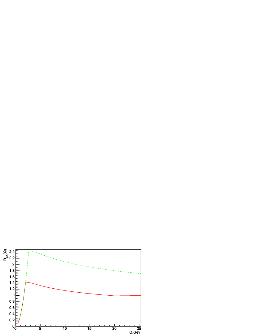
Figure 1: Cronin ratio for Kharzeev-Levin-Nardi gluon distribution function for $p+A$ collisions $\sqrt{s}=200Gev$(solid curve) and $\sqrt{s}=1700Gev$(dashed curve)

If we look at (19) we’ll see that $R_{pA}$ here is non-decreasing function of momentum $q$ so is not clean if there is any Cronin like behavior in this model. It should be mentioned however that $x$ depends on $q$ by means of relation $x=\frac{q}{\sqrt{s}}$ (if we suppose $y=0$) and as saturation momentum in low $x$ region depend on $x$ as $Q^{2}_{s}(x)=A^{1/3}Q^{2}_{s0}\left(\frac{x_{0}}{x}\right)^{\lambda}$ then in reality (19) have maximun at some monentum $q_{C}$ (figure 1) which value approximately defined by equation

$$q_{C}=Q_{s}\left(\frac{q_{C}}{\sqrt{s}}\right)$$ (20)

and modified slightly by logarifmic terms in (19). Nevertheless we have formula similair to (6):

$$\ln(q_{C})=a+b\ln(\sqrt{s})$$ (21)

where $b=0.1042$

3 McLerran-Venugopalan model

In McLerran-Venugopalan model expression for unintegrated gluon distribution function was finded in works [4, 5] and can be written as

$$\phi_{A}(x,q^{2})\,=\,\frac{4\,C_{F}}{\alpha_{s}\,(2\pi)^{3}}\,\int d^{2}b\,d^{2}r\,e^{-iq\cdot{r}}\ \frac{1}{{r}^{2}}\ (1-e^{-{r}^{2}Q_{s}^{2}\ln(1/r\Lambda)/4}),$$ (22)

Or if consider cilindrical nucleus

$$\phi_{A}(x,q^{2})\,=\,\frac{4S_{A}\,C_{F}}{\alpha_{s}\,(2\pi)^{3}}\int\,d^{2}r\,e^{-iq\cdot{r}}\ \frac{1}{{r}^{2}}\ (1-e^{-{r}^{2}Q_{s}^{2}\ln(1/r\Lambda)/4}),$$ (23)

or

$$\phi_{A}(x,q^{2})\,=\,\frac{4S_{A}\,C_{F}}{\alpha_{s}\,(2\pi)^{2}}\int\,dr\,J_{0}(q\cdot r)\ \frac{1}{r}\ (1-e^{-r^{2}Q_{s}^{2}\ln(1/r\Lambda)/4}),$$ (24)

It is better however use the expression proposed in [8] which relates unintegrated gluon distribution function in McLerran-Venugopalan model and the forward amplitude of scatering $N_{G}(r,x)$ of a gluon dipole of transverse size $r$ and rapidity $y=ln(1/x)$ on nucleus. When we can rewrite previous equation in the following form:

$$\phi_{A}(x,q^{2})\,=\,\frac{4S_{A}\,C_{F}}{\alpha_{s}\,(2\pi)^{2}}\int\,dr\,J_{0}(q\cdot r)\ \frac{1}{r}\ N_{G}(r,x),$$ (25)

where $J_{0}(x)$ is Bessel function. It obvious that $N_{G}$ depends on $x$. There are different ways to set this dependence. We can use Balitsky-Kovchegov equation to define $x$ dependence of dipole scattering cross-section but as it is unsolved for now we choise more simple way. Let us define ad hoc that

$$N_{G}(r,x)=1-e^{-r^{2}Q_{s}(x)^{2}ln(1/r\Lambda)/4}$$ (26)

i.e. all $x$ dependence goes in definition of $Q_{s}(x)$. But we can not use (26) directly as $N_{G}(r,x)$ have not very good behavior for large $r$( i.e. if $r\rightarrow\infty$ then $N_{G}(r,x)$ becomes negative instead of unity). So we should regularize (26) somehow. Let us regularize $N_{G}(r,x)$ by following prescription:

$$N_{G}(r,x)=1-e^{r^{2}Q_{s}(x)^{2}(ln(r\Lambda)-\sqrt{(\ln(r\Lambda))^{2}+\epsilon^{2})}+\ln(r_{0}\Lambda))/8}$$ (27)

and set $r_{0}=\frac{1}{\sqrt{e}\Lambda}$ and $\epsilon<1$(the final result does not depend on exact value of $\epsilon$, if it is not too large). It should be noted that result does not depend on regularization scheme and we could regularize $N_{G}(r,x)$ with something like this:

$$N_{G}(r,x)=1-e^{-r^{2}Q_{s}(x)^{2}ln(1/r\Lambda)/4}\ ,r<r_{0}$$ (28)

$$N_{G}(r,x)=1-e^{-r^{2}Q_{s}(x)^{2}ln(1/r_{0}\Lambda)/4}\ ,r>r_{0}$$

but this regularization is inconvenient in ”dipole” model.

Then for gluon distribution function $G(x,q^{2})$ we have:

$$xG_{A}(x,q^{2})\,=\,\frac{4S_{A}\,C_{F}}{\alpha_{s}\,(2\pi)^{3}}2\int\,dr\,(qJ_{1}(q\cdot r)-\Lambda J_{1}(\Lambda\cdot r))\ \frac{1}{r^{2}}\ N_{G}(r,x)),$$ (29)

If we substitute this functions in Cronin ratio (15) we’ll have dependence which is presented in figure 2. Then we can calculate numericaly value of Cronin momentum $q_{C}$ for different energies. The result is presented in figure 4. The slope is $b=0.1323$. It should be mentioned that even the line have different position they have almost the same slope as previous model and almost exactly equal one which was calculated in (7).

4 ”Dipole” model

In ”dipole” model we can relate unintegrated gluon distribution function with gluon dipole cross-section. It was done in work [6, 7] and expression for unintegrated gluon distribution function can be written as (we supposed that nucleus is cilindrical)

$$\phi_{A}(x,q^{2})\,=\,\frac{4S_{A}\,C_{F}}{\alpha_{s}\,(2\pi)^{3}}\int\,d^{2}r\,e^{-iq\cdot{r}}\ \nabla^{2}_{r}\ N_{G}(r,x)),$$ (30)

or

$$\phi_{A}(x,q^{2})\,=\,\frac{4S_{A}\,C_{F}}{\alpha_{s}\,(2\pi)^{2}}\int\,dr\,J_{0}(q\cdot r)\ r\nabla^{2}_{r}\ N_{G}(r,x),$$ (31)

For for gluon distribution function $G(x,q^{2})$ we’ll have

$$xG_{A}(x,q^{2})\,=\,\frac{4S_{A}\,C_{F}}{\alpha_{s}\,(2\pi)^{2}}2\int\,dr\,(qJ_{1}(q\cdot r)-\Lambda J_{1}(\Lambda\cdot r))\ \nabla^{2}_{r}N_{G}(r,x),$$ (32)

As before it is easy to calculate numerically value of Cronin ratio. Result is presented on figure 3. Varying energy we calculate numerically Cronin momentum $q_{C}$ (result presented on figure 4). And as before we have dependence $\ln(q_{C})=a+b\ln(\sqrt{s})$, with slope $b=0.1120$

5 A+A collisions

Like in $p+A$ collision in $A+A$ collisions(we take only central rapidity region) there is only one semihard scale $Q_{s}$. Ant therefore dependence of Cronin momentum $q_{C}$ must be govered by (3). We can apply all formulas above to this case, as we have for Cronin ratio following approximate relation similair to (15)

$$R_{A}A=\frac{G_{A}(x,p)}{G_{p}(x.p)}\frac{\phi_{A}(x,p)}{\phi_{p}(x,p)}$$ (33)

calculating numerically $q$ dependence of Cronin ration for considered models (figures 5,6,7) at differen energies we have same linear behavior for $ln(q_{C})$ as before (figure 8) and also have slopes consistent with (7). All data summarized in Table 1 (for ’dipole’ model only points with $\sqrt{s}>500Gev$ was taked for slope calculation).

	$p+A$	$A+A$
Model
Kharzeev-Levin-Nardi	0.1042	0.1485
McLerran-Venugopalan	0.1323	0.1383
’Dipole’	0.1120	0.1244

Table 1: Summary of slopes for different models in $p+A$ and $A+A$ collisions.

6 Conclusion

We calculate $\sqrt{s}$ dependence of Cronin momentum in several models based on saturation and show that this dependence is consistent with simple formula based on geometric scaling only. This subtle prediction can test validity of saturation model. Even more. As slope values is slightly different we have posibility to distinguish among variants. But this requires more precice measurement of Cronin effect(at least in midle momentum region) that those we have today. Having this we can in turn measure dependence of saturation momentum $Q_{s}(x)$ on $x$.

Figure 2: Cronin ratio for McLerran-Venucopalan gluon distribution function for $p+A$ collisions for $\sqrt{s}=200Gev$(solid curve) and $\sqrt{s}=1700Gev$ (dashed curve)

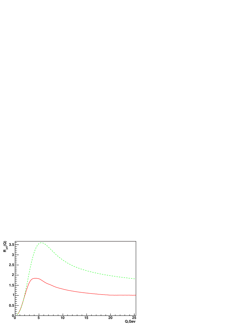
Figure 3: Cronin ratio for ”dipole” gluon distribution function for $p+A$ collisions for $\sqrt{s}=200Gev$(soild curve) and $\sqrt{s}=1700Gev$ (dashed curve)

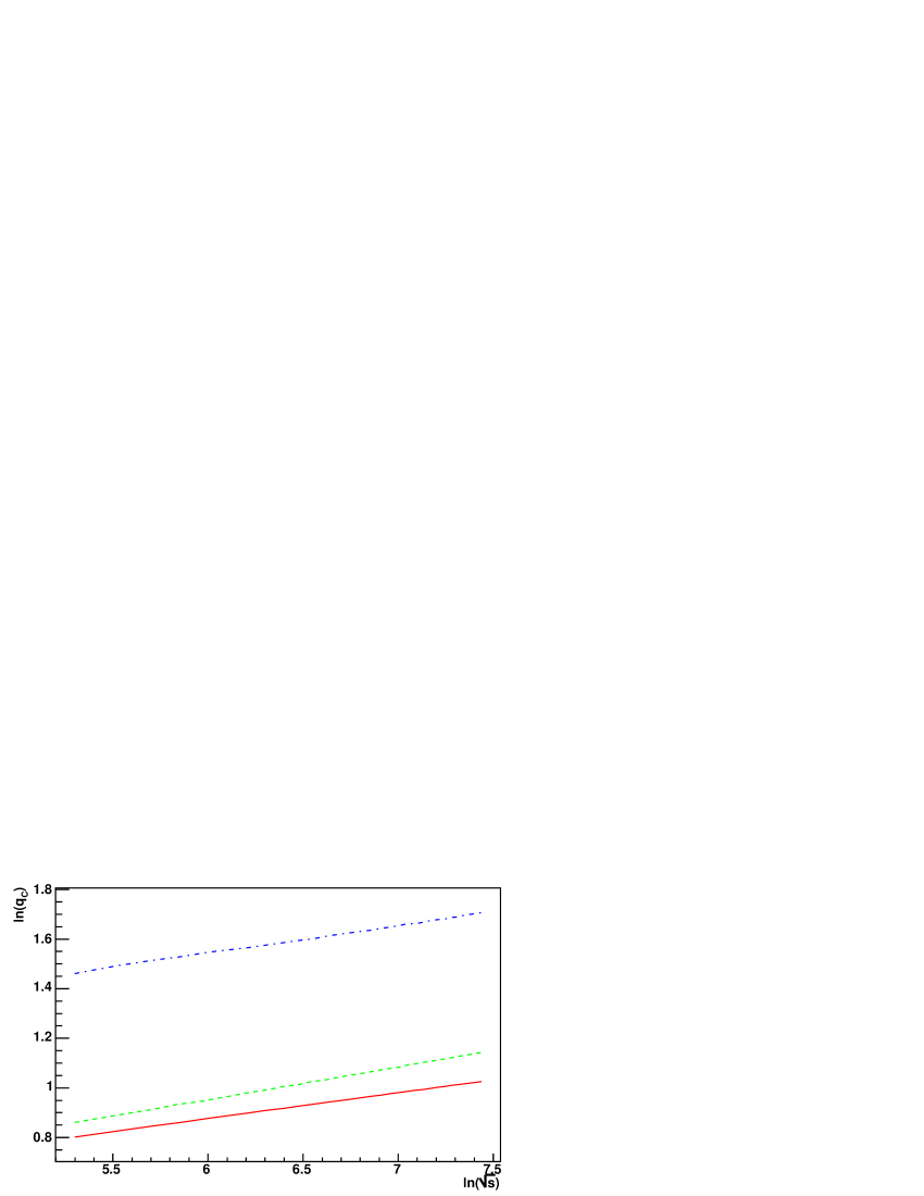
Figure 4: Dependence of $ln(q_{C})$(for $R_{pA}$)on $ln(\sqrt{s})$ for different models: Kharzeev-Levin-Nardi(solid curve), McLerran-Venugopalan(dashed curve), ”dipole” (dot-dashed curve)

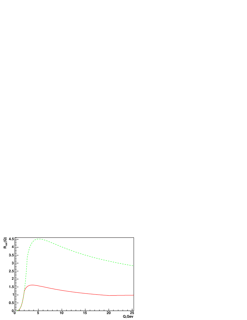
Figure 5: Cronin ratio for Kharzeev-Levin-Nardi gluon distribution function for $A+A$ collisions $\sqrt{s}=200Gev$(solid curve) and $\sqrt{s}=1700Gev$(dashed curve)

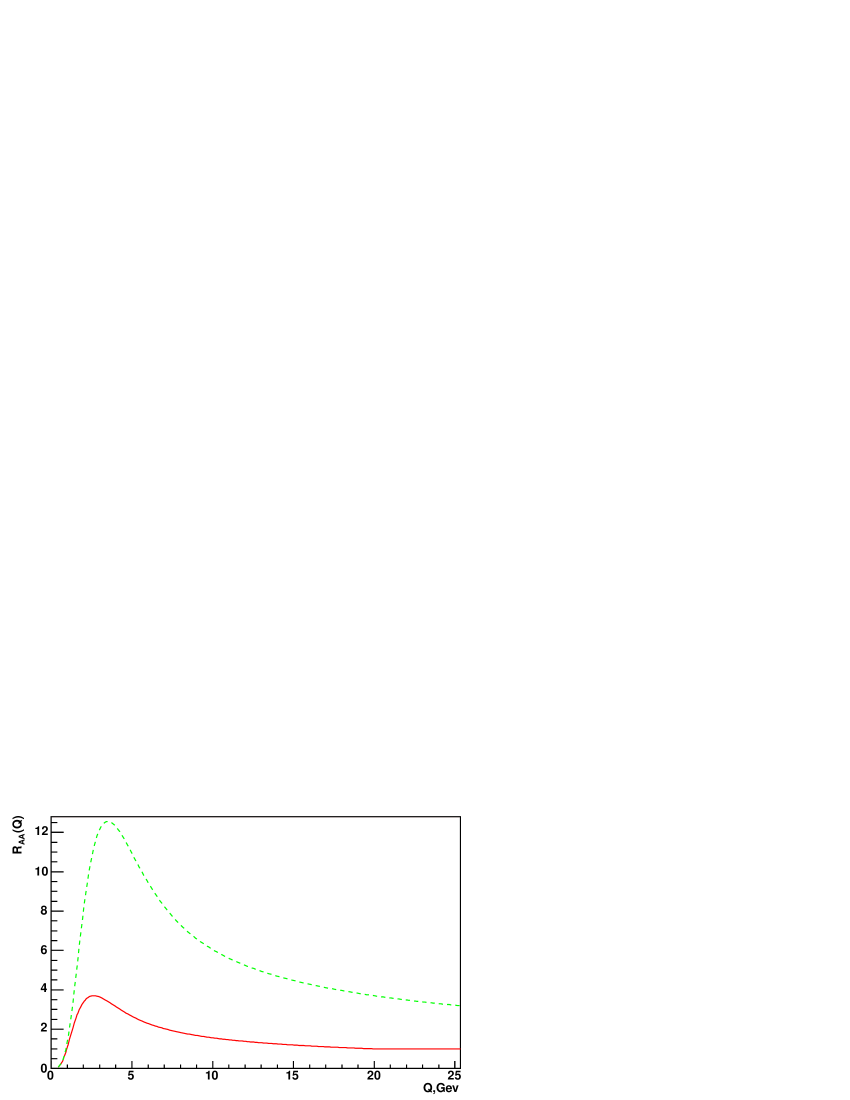
Figure 6: Cronin ratio for McLerran-Venucopalan gluon distribution function for $A+A$ collisions for $\sqrt{s}=200Gev$(solid curve) and $\sqrt{s}=1700Gev$ (dashed curve)

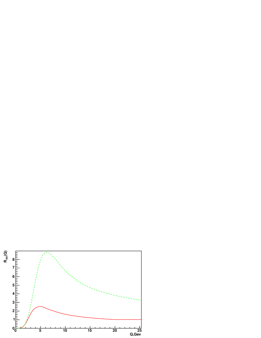
Figure 7: Cronin ratio for ”dipole” gluon distribution function for $A+A$ collisions for $\sqrt{s}=200Gev$(solid curve) and $\sqrt{s}=1700Gev$ (dashed curve)

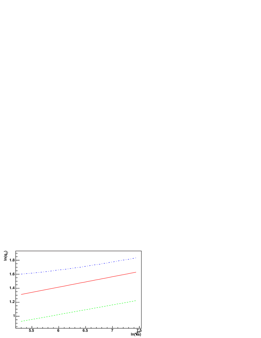
Figure 8: Dependence of $ln(q_{C})$(for $R_{AA}$) on $ln(\sqrt{s})$ for different models: Kharzeev-Levin-Nardi(solid curve), McLerran-Venugopalan(dashed curve), ”dipole” (dot-dashed curve)

References

- [1] R. Baier, A. Kovner and U. A. Wiedemann, Phys. Rev. D 68, 054009 (2003) [arXiv:hep-ph/0305265].
- [2] D. Kharzeev, E. Levin and M. Nardi, arXiv:hep-ph/0212316.
- [3] L. V. Gribov, E. M. Levin and M. G. Ryskin, Phys. Rept. 100, 1 (1983).
- [4] Y. V. Kovchegov, Phys. Rev. D 54, 5463 (1996) arXiv:hep-ph/9605446; Phys. Rev. D 55, 5445 (1997) arXiv:hep-ph/9701229; J. Jalilian-Marian, A. Kovner, L. D. McLerran and H. Weigert, Phys. Rev. D 55, 5414 (1997) arXiv:hep-ph/9606337.
- [5] Yu. V. Kovchegov and A. H. Mueller, Nucl. Phys. B 529, 451 (1998) arXiv:hep-ph/9802440.
- [6] M. Braun, Eur. Phys. J. C 16, 337 (2000)
- [7] M. A. Braun, Phys. Lett. B 483, 105 (2000)
- [8] D. Kharzeev, Y. V. Kovchegov and K. Tuchin, arXiv:hep-ph/0307037.