Day-night effect in solar neutrino oscillations with three flavors

Abstract

We investigate the effects of a nonzero leptonic mixing angle $\theta_{13}$ on the solar neutrino day-night asymmetry. Using a constant matter density profile for the Earth and well-motivated approximations, we derive analytical expressions for the $\nu_{e}$ survival probabilities for solar neutrinos arriving directly at the detector and for solar neutrinos which have passed through the Earth. Furthermore, we numerically study the effects of a non-zero $\theta_{13}$ on the day-night asymmetry at detectors and find that they are small. Finally, we show that if the uncertainties in the parameters $\theta_{12}$ and $\Delta m^{2}$ as well as the uncertainty in the day-night asymmetry itself were much smaller than they are today, this effect could, in principle, be used to determine $\theta_{13}$.

I Introduction

Neutrino oscillation physics has entered the era of precision measurements with the results from the Super-Kamiokande Fukuda et al. (1998), SNO Ahmad et al. (2001, 2002a, 2002b); Ahmed et al. , and KamLAND Eguchi et al. (2003) experiments. Especially, impressiver results have recently come from measurements of solar neutrinos (see Refs. Ahmad et al. (2002b); Ahmed et al. ; Smy et al. ) and the solar neutrino problem has successfully been solved in terms of solar neutrino oscillations.

The solar neutrino day-night effect, which measures the relative difference of the electron neutrinos coming from the Sun at nighttime and daytime, is so far the best long baseline experiment that can measure the matter effects on the neutrinos, the so-called Mikheyev-Smirnov-Wolfenstein (MSW) effect Wolfenstein (1978). In all accelerator long baseline experiments, the neutrinos cannot be made to travel through vacuum. The atmospheric neutrino experiments, on the other hand, use different baseline lengths for neutrinos traversing the Earth and those that pass through vacuum. With the advent of the precision era in neutrino oscillation physics, we can gradually hope to obtain better measurements of the day-night effect. Recently, both Super-Kamiokande and SNO have presented new measurements Ahmad et al. (2002b); Smy et al. of this effect that have errors approaching a few standard deviations in significance.

In this paper we analyze the day-night effect in the three neutrino flavor case. Earlier analyses of this effect, with a few exceptions, have been performed for the two neutrino flavor case. Furthermore, the present data also permit a new treatment of the effect due to the particular values of leptonic mixing angles and neutrino mass squared differences obtained from other experiments. There are six parameters that describe the neutrinos in the minimal extension of the standard model: three leptonic mixing angles $\theta_{12}$, $\theta_{13}$, and $\theta_{23}$, one CP-phase $\delta$, and two neutrino mass squared differences $\Delta M^{2}=m_{3}^{2}-m_{1}^{2}$ and $\Delta m^{2}=m_{2}^{2}-m_{1}^{2}$. The solar neutrino day-night effect is mainly sensitive to the angles $\theta_{12}$ and $\theta_{13}$, and the mass squared difference $\Delta m^{2}$. Our goal is to obtain a relatively simple analytic expression for the day-night asymmetry that reproduces the main features of the situation. It turns out that one can come a long way towards this goal.

Earlier treatments of the day-night effect can be found in Refs. Carlson (1986); Lisi and Montanino (1997); Guth et al. (1999); Dighe et al. (1999); Gonzalez-Garcia et al. (2001); de Holanda and Smirnov ; Bandyopadhyay et al. . Our three flavor treatment is consistent with the modifications presented by de Holanda and Smirnov de Holanda and Smirnov as well as Bandyopadhyay et al. Bandyopadhyay et al. .

This paper is organized as follows. In Sec. II we investigate the electron neutrino survival probability with $n$ flavors for solar neutrinos arriving at the Earth and for solar neutrinos going through the Earth. Next, in Sec. III we study the case of three neutrino flavors, including production and propagation in the Sun as well as propagation in the Earth. At the end of this section, we present the analytical expression for the day-night asymmetry. Then, in Sec. IV we discuss the day-night effect at detectors. Especially, we calculate the elastic scattering day-night asymmetry at the Super-Kamiokande experiment and the charged-current day-night asymmetry at the SNO experiment. Furthermore, we discuss the possibility of determining the leptonic mixing angle $\theta_{13}$ using the day-night asymmetry. In Sec. V we present our summary as well as our conclusions. Finally, in the Appendix we shortly review for completeness the day-night asymmetry in the case of two neutrino flavors.

II The $\boldsymbol{n}$ flavor solar neutrino survival probability

Assuming an incoherent neutrino flux Guth et al. (1999); Dighe et al. (1999), the $\nu_{e}$ survival probability for solar neutrinos is

$$P_{S}=\sum_{i=1}^{n}k_{i}|\left\langle\nu_{e}|\nu_{i}\right\rangle|^{2}=\sum_{i=1}^{n}k_{i}|U_{ei}|^{2},$$ (1)

where $n$ is the number of neutrino flavors and $k_{i}$ is the fraction of the mass eigenstate $\left|\nu_{i}\right\rangle$ in the flux of solar neutrinos. From unitarity it follows that

$$\sum_{i=1}^{n}k_{i}=1.$$ (2)

In the case of even mixing, i.e., $k_{i}=1/n$ for all $i$, we obtain $P_{S}=1/n$.

For neutrinos reaching the Earth during daytime (at the detector site), $P_{S}$ is the $\nu_{e}$ survival probability at the detector. However, during nighttime this survival probability may be altered by the influence of the effective Earth matter density potential. Thus, in this case, the survival probability becomes

$$P_{SE}=\sum_{i=1}^{n}k_{i}|\left\langle\nu_{e}|\tilde{\nu}_{i}\right\rangle|^{2},$$ (3)

where $\left|\tilde{\nu_{i}}\right\rangle=\left|\nu_{i}(L)\right\rangle$ and $L$ is the length of the neutrino path through the Earth. Here, the components of $\left|\nu_{i}(t)\right\rangle$ satisfy the Schrödinger equation

$$\mathrm{i}\frac{\mathrm{d}\left|\nu_{i}(t)\right\rangle_{m}}{\mathrm{d}t}=H_{m}\left|\nu_{i}(t)\right\rangle_{m}$$ (4)

with the initial condition $\left|\nu_{i}(0)\right\rangle=\left|\nu_{i}\right\rangle$ and where $m$ denotes the mass eigenstate basis.

The Hamiltonian $H$ is given by (assuming $k$ sterile neutrino flavors)

$$H_{m}\simeq\frac{M^{2}}{2p}+U^{\dagger}{\rm diag}(V_{CC},0,\ldots,0,\overbrace{-V_{NC},\ldots,-V_{NC}}^{k\ {\rm times}})U,$$ (5)

where $M={\rm diag}(m_{1},m_{2},\ldots,m_{n})$, the effective charged-current Earth matter density potential is $V_{CC}=\sqrt{2}G_{F}N_{e}$, and the effective neutral-current Eath matter density potential is $V_{NC}=-G_{F}N_{n}/\sqrt{2}$, where $G_{F}$ is the Fermi coupling constant and where $N_{e}$ and $N_{n}$ are the electron and nucleon number densities, respectively. The number densities are functions of $t$ depending on the Earth matter density profile, which is normally given by the Preliminary Reference Earth Model (PREM) Dziewonski and Anderson (1981). The term $|\left\langle\nu_{e}|\tilde{\nu_{i}}\right\rangle|^{2}$ is interpreted as the probability of a neutrino reaching the Earth in the mass eigenstate $\left|\nu_{i}\right\rangle$ to be detected as an electron neutrino after traversing the distance $L$ in the Earth. For notational convenience we denote

$$P_{ie}=|\left\langle\nu_{e}|\tilde{\nu_{i}}\right\rangle|^{2}.$$ (6)

Clearly, $P_{ie}(L=0)=|\left\langle\nu_{e}|\nu_{i}\right\rangle|^{2}=|U_{ei}|^{2}$. Furthermore, from unitarity it follows that

$$\sum_{i=1}^{n}P_{ie}=1.$$ (7)

Again, in the case of even mixing, we obtain $P_{SE}=1/n$, and the $\nu_{e}$ survival probability is unaffected by the passage through the Earth.

III The case of three neutrino flavors

Until now most analyses of the day-night effect have been done in the framework of two neutrino flavors. However, we know that there are (at least) three neutrino flavors. The reason for using two flavor analyses has been that the leptonic mixing angle $\theta_{13}$ is known to be small Apollonio et al. (1999), leading to an approximate two neutrino case. One of the main goals of this paper is to find the effects on the day-night asymmetry induced by using a non-zero mixing angle $\theta_{13}$. In what follows, we assume that there are three active neutrino flavors and no sterile neutrinos.

We will use the standard parametrization of the $3\times 3$ leptonic mixing matrix Hagiwara et al. (2002)

$$U=\left(\begin{array}[]{ccc}c_{13}c_{12}&c_{13}s_{12}&s_{13}{\rm e}^{-{\rm i}\delta}\\ &*&*\\ &*&*\end{array}\right),$$ (8)

where $s_{ij}=\sin\theta_{ij}$ and $c_{ij}=\cos\theta_{ij}$, $\theta_{ij}$ are leptonic mixing angles, and the elements denoted by $*$ do not affect the neutrino oscillation probabilities, which we are calculating in this paper.

III.1 Production and propagation in the Sun

In the three flavor framework, there are a number of issues of the neutrino production and propagation in the Sun, which are not present in the two flavor framework. First of all, the three energy levels of neutrino matter eigenstates in general allow two MSW resonances. Furthermore, the matter dependence of the mixing parameters are far from as simple as in the two flavor case. The result of this is that we have to make certain approximations.

Repeating the approach made in the two flavor case (see the Appendix), we obtain the following expression for $k_{i}$:

$$k_{i}=\int_{0}^{R_{\odot}}\mathrm{d}rf(r)\sum_{j=1}^{3}|\hat{U}_{ej}|^{2}P_{ji}^{s},$$ (9)

where $\hat{U}$ is the mixing matrix in matter, $P_{ji}^{s}$ is the probability of a neutrino created in the matter eigenstate $\left|\nu_{M,j}\right\rangle$ to exit the Sun in the mass eigenstate $\left|\nu_{i}\right\rangle$, and $f(r)$ is the normalized spatial production distribution in the Sun.

The second resonance in the three flavor case occurs at $V_{CC}\simeq\cos(2\theta_{13}){\Delta M^{2}}/{(2E)}$, assuming that the resonances are fairly separated. The maximal electron number density in the Sun, according to the standard solar model (SSM) Bahcall et al. (2001), is about $N_{e,\rm max}\simeq 102$ $N_{A}$/cm³, yielding a maximal effective potential $V_{CC,\mathrm{max}}\simeq 7.8\times 10^{-18}$ MeV. Assuming the large mass squared difference $\Delta M^{2}$ to be of the order of the atmospheric mass squared difference ($|\Delta m_{\mathrm{atm}}^{2}|\simeq 2\times 10^{-3}$ eV² Maltoni et al. (2003)), the neutrino energy $E$ to be of the order of $10$ MeV, and $\theta_{13}$ to be small, we find $\left|{\Delta M^{2}}/{2E}\right|\cos(2\theta_{13})\simeq 10^{-16}$ MeV. Thus, the solar neutrinos never pass through the second resonance, independent of the sign of the large mass squared difference.

Since the neutrinos never pass through the second resonance, it is a good approximation to assume that the matter eigenstate $\left|\nu_{M,3}\right\rangle$ evolves adiabatically, and thus, we have

$$P_{3k}^{s}=P_{k3}^{s}=\delta_{3k}.$$ (10)

Unitarity then implies that

$$P_{12}^{s}=P_{21}^{s}=P_{\rm jump}.$$ (11)

Furthermore, if we assume that $V_{CC}\lesssim{\Delta m^{2}}/{(2E)}\ll{\Delta M^{2}}/{(2E)}$, the neutrino evolution is well approximated by the energy eigenstate $\left|\nu_{M,3}\right\rangle$ evolving as the mass eigenstate $\left|\nu_{3}\right\rangle$ and the remaining neutrino states oscillating according to the two flavor case with the effective potential $V_{\mathrm{eff}}=c_{13}^{2}V_{CC}$. This does not change the probability $P_{\rm jump}$ as calculated with a linear approximation of the potential in the two flavor case. This means that we may use the same expression as that obtained in the two flavor case, see the Appendix, even if the resonance point, where $|{N_{e}}/{\dot{N}_{e}}|$ is to be evaluated, does change. However, in the Sun, $N_{e}$ is approximately exponentially decaying with the radius of the Sun, leading to $|{N_{e}}/{\dot{N}_{e}}|$ being approximately constant, and thus, independent of the point of evaluation. For the large mixing angle (LMA) region, the probability $P_{\rm jump}$ of a transition from $\left|\nu_{M,1}\right\rangle$ to $\left|\nu_{M,2}\right\rangle$, or vice versa, is negligibly small ($P_{\rm jump}<10^{-1700}$). However, we keep it in our formulas for completeness.

To make one further approximation, as long as the Sun’s effective potential is much less than the large mass squared difference $\Delta M^{2}$, the mixing angle $\hat{\theta}_{13}\simeq\theta_{13}$ giving

$$k_{3}\simeq\int_{0}^{R_{\odot}}\mathrm{d}rf(r)\sin^{2}\theta_{13}=\sin^{2}\theta_{13}.$$ (12)

A general parametrization for $k_{1}$ and $k_{2}$ is then given by

$$k_{1}=c_{13}^{2}\frac{1+D_{3\nu}}{2},\ \ k_{2}=c_{13}^{2}\frac{1-D_{3\nu}}{2}.$$ (13)

In the above approximation, the oscillations between the matter eigenstates $\left|\nu_{M,1}\right\rangle$ and $\left|\nu_{M,2}\right\rangle$ are well approximated by a two flavor oscillation, using the small mass difference squared $\Delta m^{2}$, the mixing angle $\theta_{12}$, and the effective potential $V_{\mathrm{eff}}=c_{13}^{2}V_{CC}$. Thus, we obtain

$$D_{3\nu}=\int_{0}^{R_{\odot}}\mathrm{d}rf(r)\cos[2\hat{\theta}_{12}(r)](1-2P_{\rm jump}),$$ (14)

where $\cos[2\hat{\theta}_{12}(r)]$ is calculated in the same way as in the two flavor case using the effective potential. For reasonable values of the neutrino oscillation parameters, this turns out to be an excellent approximation.

Inserting the above approximation into Eq. (1) with $n=3$, we obtain

$$P_{S}=s_{13}^{4}+c_{13}^{4}\frac{1+D_{3\nu}\cos(2\theta_{12})}{2}.$$ (15)

When $\theta_{13}\rightarrow 0$, we have $D_{3\nu}\rightarrow D_{2\nu}$, and thus, we recover the two flavor survival probability in this limit.

III.2 Propagation in the Earth

As in the case of propagation in the Sun, $V_{CC}\lesssim{\Delta m^{2}}/{2E}\ll{\Delta M^{2}}/{2E}$, $\left|\nu_{M,3}\right\rangle\simeq\left|\nu_{3}\right\rangle$, and the remaining two neutrino eigenstates evolve according to the two flavor case with an effective potential of $V_{\mathrm{eff}}=c_{13}^{2}V_{CC}$. For the MSW solutions of the solar neutrino problem along with the assumption that $\Delta M^{2}$ is of the same order of magnitude as the atmospheric mass squared difference, this condition is well fulfilled for solar neutrinos propagating through the Earth. As a direct result, we obtain the probability $P_{3e}$ as

$$P_{3e}\simeq|\left\langle\nu_{e}|\nu_{3}\right\rangle|^{2}=|U_{e3}|^{2}=s_{13}^{2}.$$ (16)

It also follows that

$$P_{2e}=c_{13}^{4}\frac{KV_{E}}{4a^{2}}\sin^{2}(2\theta_{12})\sin^{2}(aL)+c_{13}^{2}s_{12}^{2},$$ (17)

where

$$a=\frac{1}{2}\sqrt{K^{2}-2c_{13}^{2}V_{E}K\cos(2\theta_{12})+c_{13}^{4}V_{E}^{2}},$$ (18)

$V_{E}$ is the electron neutrino potential in the Earth, and $K={\Delta m^{2}}/{2E}$. We observe that when $L=0$ or $V_{E}=0$, $P_{2e}=c_{13}^{2}s_{12}^{2}=|U_{e2}|^{2}$ just as expected.

III.3 The final expression for $\boldsymbol{P}_{\boldsymbol{n-d}}$

Now, we insert the analytical expressions obtained in the previous two sections into Eq. (3) with $n=3$ and subtract $P_{S}$ from this in order to obtain an expression for $P_{n-d}=P_{SE}-P_{S}$ in the three flavor framework. After some simplifications, we find

$$P_{n-d}=-c_{13}^{6}D_{3\nu}\frac{KV_{E}}{4a^{2}}\sin^{2}(2\theta_{12})\sin^{2}(aL).$$ (19)

For the MSW solutions of the solar neutrino problem, $K\gg c_{13}^{2}V_{E}$, and thus, $a\simeq K/2$. This yields

$$P_{n-d}\simeq-2c_{13}^{6}D_{3\nu}\frac{EV_{E}}{\Delta m^{2}}\sin^{2}(2\theta_{12})\sin^{2}\left({\textstyle\frac{\Delta m^{2}}{4E}L}\right).$$ (20)

Apparently, the effect of using three flavors instead of two is, up to the approximations made, a multiplication by $c_{13}^{6}$ as well as a correction in changing $D_{2\nu}$ to $D_{3\nu}$. When $\theta_{13}\rightarrow 0$, we have $D_{3\nu}\rightarrow D_{2\nu}$, and we regain the two flavor expression in this limit (see the Appendix). An important observation is that the regenerative term, for $V_{E}\ll K$, is linearly dependent on $V_{E}$. Thus, the choice of which value of $V_{E}$ to use is crucial for the quantitative result. As is argued in the appendix, the potential to use is the potential corresponding to the electron number density of the Earth’s crust. However, the qualitative behavior of the effect of a non-zero $\theta_{13}$ is not greatly affected.

IV The day-night effect at detectors

From the calculations made in the previous parts of this paper, we obtain the day-night asymmetry of the electron neutrino flux at the neutrino energy $E$ as

$$A_{n-d}^{\phi_{e}}(E) = 2\frac{\phi_{e,N}(E)-\phi_{e,D}(E)}{\phi_{e,N}(E)+\phi_{e,D}(E)}$$ (21)

$$= \frac{P_{n-d}(E)}{P_{S}(E)+\frac{P_{n-d}(E)}{2}}.$$

However, this is not the event rate asymmetry measured at detectors. We will assume a water-Cherenkov detector in which neutrinos are detected by one of the following reactions :

$$\nu_{x}+e^{-} \longrightarrow \nu_{x}+e^{-},$$ (22)

$$\nu_{x}+d \longrightarrow p+p+e^{-},$$ (23)

where $x=e,\mu,\tau$, which are referred to as elastic scattering (ES) and charged-current (CC), respectively. The CC reaction can only occur for $x=e$, since inserting $x\neq e$ in Eq. (23) would violate the lepton numbers $L_{e}$ and $L_{x}$. We assume that the scattered electron energy $T^{\prime}$ is measured and that the cross sections ${\mathrm{d}\sigma_{\nu_{\mu}}}/{\mathrm{d}T^{\prime}}$ and ${\mathrm{d}\sigma_{\nu_{\tau}}}/{\mathrm{d}T^{\prime}}$ are equal.

If we denote the zenith angle, i.e., the angle between zenith and the Sun at the detector, by $\alpha$, then the event rate of measured electrons with energy $T$ in the detector is proportional to

$$R(\alpha,T) = \int_{0}^{\infty}\mathrm{d}E\phi(E)\int_{0}^{T^{\prime}_{\mathrm{max}}}\mathrm{d}T^{\prime}$$ (24)

$$\times F(T,T^{\prime})\frac{\mathrm{d}\sigma_{\nu_{\mathrm{solar}}}}{\mathrm{d}T^{\prime}},$$

where $\phi(E)$ is the total solar neutrino flux, $T^{\prime}$ is the true electron energy, and ${\mathrm{d}\sigma_{\nu_{\mathrm{solar}}}}/{\mathrm{d}T^{\prime}}$ is given by

$$\frac{\mathrm{d}\sigma_{\nu_{\mathrm{solar}}}}{\mathrm{d}T^{\prime}}=P_{SE}\frac{\mathrm{d}\sigma_{\nu_{e}}}{\mathrm{d}T^{\prime}}+(1-P_{SE})\frac{\mathrm{d}\sigma_{\nu_{\mu}}}{\mathrm{d}T^{\prime}}.$$ (25)

Here, we have used the assumption ${\mathrm{d}\sigma_{\nu_{\mu}}}/{\mathrm{d}T^{\prime}}={\mathrm{d}\sigma_{\nu_{\tau}}}/{\mathrm{d}T^{\prime}}$, since neutrinos not found in the state $\left|\nu_{e}\right\rangle$ are assumed to be in the state $\left|\nu_{\mu}\right\rangle$ or in the state $\left|\nu_{\tau}\right\rangle$. The energy resolution of the detector is introduced through $F(T,T^{\prime})$, which is given by

$$F(T,T^{\prime})=\frac{1}{\Delta_{T^{\prime}}\sqrt{2\pi}}\exp\left(-\frac{(T-T^{\prime})^{2}}{2\Delta_{T^{\prime}}^{2}}\right),$$ (26)

where $\Delta_{T^{\prime}}$ is the energy resolution at the electron energy $T^{\prime}$.

The night and day rates $N$ and $D$ at the measured electron energy $T$ are given by

$$D(T) = \int_{0}^{\pi/2}\mathrm{d}\alpha R(\alpha,T)Y(\alpha),$$ (27)

$$N(T) = \int_{\pi/2}^{\pi}\mathrm{d}\alpha R(\alpha,T)Y(\alpha),$$ (28)

respectively. Here, $Y(\alpha)$ is the zenith angle exposure function, which gives the distribution of exposure time for the different zenith angles. The exposure function is clearly symmetric around $\alpha=\pi/2$ and is plotted in Fig. 1 for both Super-Kamiokande (SK) and SNO.

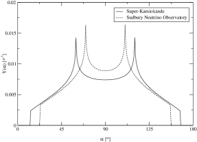
Figure 1: The zenith angle exposure function $Y(\alpha)$ for SK and SNO as a function of the zenith angle $\alpha$. The data are retrieved from Ref. Bah .

From the night and day rates at a specific electron energy, we define the day-night asymmetry at energy $T$ as

$$A_{n-d}(T)=2\frac{N(T)-D(T)}{N(T)+D(T)}.$$ (29)

The final day-night asymmetry is given by integrating the day and night rates over all energies above the detector threshold energy $T_{\rm th}$, i.e.,

$$A_{n-d}=2\frac{\int_{T_{\mathrm{th}}}^{\infty}\mathrm{d}T[N(T)-D(T)]}{\int_{T_{\mathrm{th}}}^{\infty}\mathrm{d}T[N(T)+D(T)]}=2\frac{N-D}{N+D}.$$ (30)

The threshold energy $T_{\mathrm{th}}$ is 5 MeV for both SK and SNO.

For computational reasons, we will start by performing the integral over the zenith angle $\alpha$. For the daytime flux $D$, $P_{SE}=P_{S}$, which is independent of $\alpha$. As a result, the only $\alpha$ dependence is in $Y(\alpha)$ and the zenith angle integral only contributes with a factor one-half [if the normalization of $Y$ is such that $\int_{0}^{\pi}\mathrm{d}\alpha Y(\alpha)=1$]. In order to be able to use the results we have obtained for $P_{n-d}$, we need to compute the difference between the night and day fluxes, which is given by

$$N(T)-D(T)=\int_{\pi/2}^{\pi}\mathrm{d}\alpha Y(\alpha)R^{n-d},$$ (31)

where the quantity $R^{n-d}=R(\alpha,T)-R(\pi-\alpha,T)$ is on the form

$$R^{n-d} = \int_{0}^{\infty}\mathrm{d}E_{\nu}\phi(E_{\nu})\int_{0}^{T^{\prime}_{\mathrm{max}}}\mathrm{d}T^{\prime}$$ (32)

$$\times F(T,T^{\prime})\frac{\mathrm{d}\sigma_{\nu_{\mathrm{sol}}}^{n-d}}{\mathrm{d}T^{\prime}}$$

and

$$\frac{\mathrm{d}\sigma_{\nu_{\mathrm{sol}}}^{n-d}}{\mathrm{d}T^{\prime}}=P_{n-d}(\alpha,E_{\nu})\left(\frac{\mathrm{d}\sigma_{\nu_{e}}}{\mathrm{d}T^{\prime}}-\frac{\mathrm{d}\sigma_{\nu_{\mu}}}{\mathrm{d}T^{\prime}}\right).$$ (33)

Note that the $\alpha$ dependence in $P_{n-d}$ enters through the length traveled by the neutrinos in the Earth and that the argument $aL$ of the second $\sin^{2}$ factor in Eq. (19) oscillates very fast and performs an effective averaging of $P_{n-d}$ in the zenith angle integral, i.e., replacing $\sin^{2}(aL)$ by $1/2$. After this averaging, the only zenith angle dependence left is that of $Y(\alpha)$ and the zenith angle integral only gives us a factor of one-half as in the case of the day rate $D$.

IV.1 Elastic scattering detection

Neutrinos are detected through ES at both SK and SNO. The ES cross sections in the laboratory frame are given by Ref. Hagiwara et al. (2002). For kinematical reasons, the maximal kinetic energy of the scattered electron in the laboratory frame is given by

$$T^{\prime}_{\mathrm{max}}=\frac{E_{\nu}}{1+\frac{m_{e}}{2E_{\nu}}}.$$ (34)

The integrals that remain cannot be calculated analytically. Hence, we use numerical methods to evaluate these integrals. However, computing all integrals by numerical methods demands a lot of computer time, and thus, we make one further approximation, that all solar ⁸B neutrinos are produced where the solar effective potential is $V_{CC}\simeq 7.07\times 10^{-18}$ MeV, which is the effective potential at the radius where most solar neutrinos are produced. For reasonable values of the fundamental neutrino parameters, the error made in this approximation is small.

For the energy resolution of SK, we use Guth et al. (1999)

$$\Delta_{T^{\prime}}=1.6\ \mathrm{MeV}\sqrt{T^{\prime}/(10\ \mathrm{MeV})},$$ (35)

and for the electron number density in the Earth, we use $N_{e}=1.4N_{A}$/cm³, where $N_{A}$ is the Avogadro constant, which roughly corresponds to 2.8 g/cm³ (using $Z/A\simeq 0.5$, where $Z$ is the number of protons and $A$ the number of nucleons for the mantle of the Earth). The electron number density used corresponds to the density in the Earth’s crust. The motivation for using this density rather than a mean density can be found in the Appendix. Note that the regenerative term $P_{n-d}$ in Eq. (20), and thus, the day-night asymmetry, is linearly dependent on the matter potential $V_{E}$. It follows that the electron number density used has a great impact on the final results. If we had used the average mantle matter density of about 5 g$/$cm³, then the resulting asymmetry would increase by almost a factor of two.

The above values give us the numerical results presented in Fig. 2.

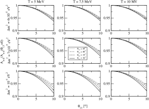
Figure 2: The day-night asymmetry at SK for different values of $T$, $\Delta m^{2}$, and $\theta_{12}$ as a function of $\theta_{13}$ relative to the corresponding value for $\theta_{13}=0$.

As can be seen from this figure, the relative effect of a non-zero $\theta_{13}$ is increasing if the small mass squared difference $\Delta m^{2}$ increases or if the measured electron energy or the leptonic mixing angle $\theta_{12}$ decreases. The effect of changing $\theta_{12}$ is also clearly larger for smaller electron energy $T$ and larger small mass squared difference $\Delta m^{2}$. In Fig. 3 the isocontours of constant day-night asymmetry in the SK detector with $\theta_{13}$ equal to 0, $9.2^{\circ}$ and $12^{\circ}$ are shown for a parameter space covering the LMA solution of the solar neutrino problem. The values used for $\theta_{13}$ correspond to no mixing as well as the CHOOZ upper bound for $\Delta M^{2}$ equal to $2.5\times 10^{-3}$ eV² and $2.0\times 10^{-3}$ eV², respectively Apollonio et al. (2003).

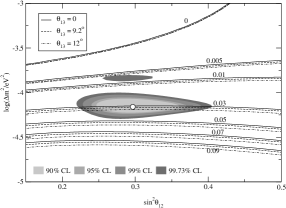
Figure 3: Isocontours in the $\theta_{12}$-$\Delta m^{2}$ parameter space for the ES day-night asymmetry for three different values of $\theta_{13}$. The values of $A_{n-d}$ for the different isocontours are shown in the figure. The shaded regions correspond to the allowed regions of the parameter space for different confidence levels and the circle corresponds to the best-fit point according to Ref. Maltoni et al. (2003).

As can be seen from this figure, the variation in the isocontours are small compared to the size of the LMA solution and to the current uncertainty in the day-night asymmetry Ahmad et al. (2002b); Smy et al. . However, if the values of the parameters $\theta_{12}$, $\Delta m^{2}$, and $A_{n-d}$ were known with a larger accuracy, then the change due to non-zero $\theta_{13}$ could, in principle, be used to determine the “reactor” mixing angle $\theta_{13}$ as an alternative to long baseline experiments such as neutrino factories Huber et al. (2002); Apollonio et al. and super-beams Huber et al. (2002, 2003); Itow et al. as well as future reactor experiments Huber et al. (2003) and matter effects for supernova neutrinos Dighe et al. (2003). The day-night asymmetry for the best-fit value of Ref. Maltoni et al. (2003) is $A_{n-d}\simeq 3.0$ %, which is larger than the theoretical value quoted by the SK experiment, but still clearly within one standard deviation of the experimental best-fit value $A_{n-d}=(1.8\pm 1.6{}^{+1.2}_{-1.3})$ % Smy et al. .

IV.2 Charged-current detection

Only SNO uses heavy water, and thus, SNO is the only experimental facility detecting solar neutrinos through the CC reaction (23). Since the electron mass $m_{e}$ is much smaller than the proton mass $m_{p}$ ($m_{e}\simeq 511$ keV, $m_{p}\simeq 938$ MeV), most of the kinetic energy in the center-of-mass frame, which is well approximated by the laboratory frame, since the deuteron mass by far exceeds the neutrino momentum, after the CC reaction will be carried away by the electron. This energy is given by

$$T^{\prime}=E+\Delta E_{\mathrm{mass}},$$ (36)

where $\Delta E_{\mathrm{mass}}=m_{d}-2m_{p}-m_{e}\simeq-1.95$ MeV. Thus, we approximate the differential cross section ${\mathrm{d}\sigma_{\nu_{e}}}/{\mathrm{d}T^{\prime}}$ by

$$\frac{\mathrm{d}\sigma_{\nu_{e}}}{\mathrm{d}T^{\prime}}=\sigma_{\nu_{e}}\delta(T^{\prime}-E+1.95\ \mathrm{MeV}).$$ (37)

In the above expression, we use the numerical results given in Ref. Ando et al. (2003) and perform linear interpolation to calculate the total cross section $\sigma_{\nu_{e}}$ as a function of the neutrino energy $E$. For $x\neq e$, the reaction in Eq. (23) is forbidden, since it violates the lepton numbers $L_{e}$ and $L_{x}$. Thus, for $x\neq e$, we have ${\mathrm{d}\sigma_{\nu_{x}}}/{\mathrm{d}T^{\prime}}=0$.

The energy resolution at SNO is given by Ahmad et al. (2002a); SNO

$$\Delta_{T^{\prime}} = -0.0684\ \mathrm{MeV}$$ (38)

$$+0.331\ \mathrm{MeV}\ {\textstyle\sqrt{\left({T^{\prime}}/{\rm MeV}\right)}}$$

$$+0.0425\ {\rm MeV}\ {\textstyle\left({T^{\prime}}/{\rm MeV}\right)}.$$

This gives the results presented in Fig. 4.

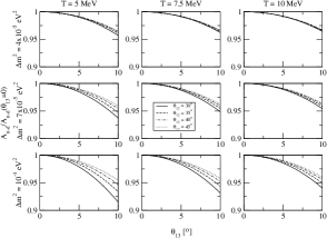
Figure 4: The CC day-night asymmetry at SNO for different values of $T$, $\Delta m^{2}$, and $\theta_{12}$ as a function of $\theta_{13}$ relative to the corresponding value for $\theta_{13}=0$.

This figure shows the same main features as Fig. 2. However, the effects of different $T$ and $\Delta m^{2}$ are larger in the CC case.

In Fig 5 we have plotted isocontours for the CC day-night asymmetry for $\theta_{13}$ equal to 0, $9.2^{\circ}$ and $12^{\circ}$ in order to observe the effect of a non-zero $\theta_{13}$ for the day-night asymmetry isocontours in the region of the LMA solution.

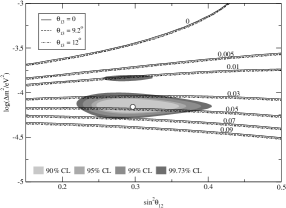
Figure 5: Isocontours for the CC day-night asymmetry in the $\theta_{12}$-$\Delta m^{2}$ parameter space for three different values of $\theta_{13}$. The values of $A_{n-d}$ for the different isocontours are shown in the figure. The shaded regions and the circle are the same as in Fig. 3.

Just as in the case of ES, the isocontours do not change dramatically and the change is small compared to the uncertainty in the day-night asymmetry. It is also apparent that the day-night asymmetry is smaller for the ES detection than for the CC detection. This is to be expected, since the ES detection is sensitive to the fluxes of $\nu_{\mu}$ and $\nu_{\tau}$ as well as to the $\nu_{e}$ flux, while the CC detection is only sensitive to the $\nu_{e}$ flux. The day-night asymmetry for the best-fit values of Ref. Maltoni et al. (2003) is $A_{n-d}\simeq 4.7\%$, which corresponds rather well to the values presented in Refs. de Holanda and Smirnov ; Bandyopadhyay et al. . The latest experimental value for the day-night asymmetry at SNO is $A_{n-d}=(7.0\pm 4.9{}^{+1.3}_{-1.2})$ % Ahmad et al. (2002b).

IV.3 Determining $\boldsymbol{\theta_{13}}$ by using the day-night asymmetry

As we observed earlier, the day-night asymmetry can, in principle, be used for determining the mixing angle $\theta_{13}$ if the experimental uncertainties in $\Delta m^{2}$, $\theta_{12}$, and the day-night asymmetry itself were known to a larger accuracy. We now ask how small the above uncertainties must be to obtain a reasonably low uncertainty in $\theta_{13}$. To estimate the uncertainty $\delta\theta_{13}$ in $\theta_{13}$, we use the pessimistic expression

$$\delta\theta_{13} \simeq {\textstyle\left|\frac{\partial\theta_{13}}{\partial A_{n-d}}\right|\delta A_{n-d}+\left|\frac{\partial\theta_{13}}{\partial\theta_{12}}\right|\delta\theta_{12}}$$ (39)

$$+{\textstyle\left|\frac{\partial\theta_{13}}{\partial\Delta m^{2}}\right|\delta\Delta m^{2}}.$$

Let us suppose that, some time in the future, we have determined the best-fit values for the parameters $\Delta m^{2}$ and $\theta_{12}$ to be $\Delta m^{2}=6.9\cdot 10^{-5}$ eV² and $\theta_{12}=33.2^{\circ}$ with the uncertainties $\delta\Delta m^{2}\simeq 2.5\cdot 10^{-6}$ eV² and $\delta\theta_{12}\simeq 0.5^{\circ}$. Furthermore, suppose that we have measured the day-night asymmetry for the ES reaction to be $A_{n-d}\simeq 0.03$ with an uncertainty $\delta A_{n-d}\simeq 0.002$. These uncertainties roughly correspond to one-tenth of the uncertainties of today’s measurements. Next, we estimate the partial derivatives of Eq. (39) numerically and obtain ${\partial\theta_{13}}/{\partial A_{n-d}}\simeq-{3000}^{\circ}$, ${\partial\theta_{13}}/{\partial\theta_{12}}\simeq 0.4$, and ${\partial\theta_{13}}/{\partial\Delta m^{2}}\simeq-2\cdot 10^{6}{{}^{\circ}}/{{\rm eV}^{2}}$. This gives an estimated error in $\theta_{13}$ of $\delta\theta_{13}\simeq 12^{\circ}$ with $6.6^{\circ}$ from the uncertainty in $A_{n-d}$, $5.2^{\circ}$ from the uncertainty in $\Delta m^{2}$ and $0.2^{\circ}$ from the uncertainty in $\theta_{12}$. (Using the uncertainties $\delta\Delta m^{2}\simeq 0.8\cdot 10^{-6}$ eV² and $\delta\theta_{12}\simeq 4^{\circ}$ suggested in Ref. Bandyopadhyay et al. (2003), we obtain the uncertainty $\delta\theta_{13}\simeq 10^{\circ}$.) Thus, the uncertainty in $\theta_{13}$ is less dependent on the uncertainty in $\theta_{12}$ than the uncertainties in $A_{n-d}$ and $\Delta m^{2}$. We observe that the precise value of the partial derivatives depend on the point of evaluation, but that the values presented give a notion about their magnitudes. If we use a more optimistic estimate instead of Eq. (39), then $\delta\theta_{13}$ reduces to about $8^{\circ}$. Unfortunately, this is still a quite large uncertainty and in order to reach an uncertainty of about $1^{\circ}$, we need measurements of $A_{n-d}$ and $\Delta m^{2}$ with uncertainties that are about 100 times smaller than the uncertainties of today and a measurement of $\theta_{12}$ with an uncertainty that is about 10 times smaller than today.

We would like to stress that the above can only be considered as an indication of the uncertainties needed to determine $\theta_{13}$ and serves mainly to present the idea of measuring $\theta_{13}$ with the solar day-night asymmetry. In a realistic scenario, uncertainties and fluctuations in the Earth matter density must be treated in a more rigorous way than using a constant Earth potential; this would probably require a full numerical simulation with three neutrino flavors.

V Summary and conclusions

We have derived analytical expressions for the day $P_{S}$ and night $P_{SE}$ survival probabilities for solar neutrinos in the case of three neutrino flavors. The analytical result has been used to numerically study the qualitative effect of a non-zero $\theta_{13}$ mixing on the day-night asymmetry $A_{n-d}$ at detectors. The regenerative term in the three flavor framework was found to be

$$P_{n-d} = -c_{13}^{6}D_{3\nu}\frac{KV_{E}}{4a^{2}}\sin^{2}(2\theta_{12})\sin^{2}(aL)$$ (40)

$$\simeq -c_{13}^{6}D_{3\nu}\frac{2EV_{E}}{\Delta m^{2}}\sin^{2}(2\theta_{12})$$

$$\times\sin^{2}\left({\textstyle\frac{\Delta m^{2}}{4E}L}\right),$$

where $K=\Delta m^{2}/(2E)$ and the approximation is good for all parts of the LMA region. We have also noted that we regain the two flavor expression for the regenerative term when $\theta_{13}\rightarrow 0$. An important observation is that the quantitative result depends linearly on the effective Earth electron density number used to calculate the regenerative term. We have argued that the value to be used is that of the Earth’s crust.

In the study of the day-night asymmetry at detectors, it is apparent that the relative effect of a non-zero $\theta_{13}$ in the LMA region is increasing for increasing $\Delta m^{2}$ and decreasing $\theta_{12}$ and measured electron energy $T$. The dependence on $\theta_{12}$ is also larger for smaller $T$ and larger $\Delta m^{2}$. This result holds for both the elastic scattering and charged-current detection of neutrinos.

We have also shown that the effects of a non-zero $\theta_{13}$ on the isocontours of constant day-night asymmetry $A_{n-d}$ at detectors are small compared to the current experimental uncertainty in $A_{n-d}$. However, should this uncertainty and the uncertainties in the fundamental parameters $\theta_{12}$ and $\Delta m^{2}$ become much smaller in the future, the day-night asymmetry could be used to determine $\theta_{13}$ as an alternative to future long baseline and reactor experiments.

Appendix A The case of two neutrino flavors

In the two flavor case, we use the parametrization

$$U=\left(\begin{array}[]{cc}c&s\\ -s&c\end{array}\right),$$ (41)

where $s=\sin\theta$ and $c=\cos\theta$ for the leptonic mixing matrix. In this case, we can also write $P_{SE}$ as a function of $P_{S}$ and $P_{2e}$ only such that

$$P_{n-d}=P_{SE}-P_{S}=\frac{1-2P_{S}}{\cos(2\theta)}(P_{2e}-\sin^{2}\theta).$$ (42)

For $k_{1}$ and $k_{2}$, a general parametrization is

$$k_{1}=\frac{1+D_{2\nu}}{2},\ \ k_{2}=\frac{1-D_{2\nu}}{2}.$$ (43)

If we assume that all transitions among the matter eigenstates are incoherent and/or negligible in magnitude, then $k_{1}$ and $k_{2}$ are also given by

$$k_{i}=\int_{0}^{R_{\odot}}\mathrm{d}rf(r)[\cos^{2}\hat{\theta}(r)P^{s}_{1i}+\sin^{2}\hat{\theta}(r)P^{s}_{2i}],$$ (44)

where $i\in\{1,2\}$, $P_{ki}^{s}$ is the probability of a neutrino in the mass eigenstate $\left|\nu_{M,k}\right\rangle$ at position $r$ to exit the Sun in the state $\left|\nu_{i}\right\rangle$, $\hat{\theta}$ is the mixing angle in matter, and $f(r)$ is the normalized spatial distribution function of the production of neutrinos. Using this, we obtain $D_{2\nu}$ as

$$D_{2\nu}=\int_{0}^{R_{\odot}}\mathrm{d}rf(r)\cos[2\hat{\theta}(r)](1-2P_{\rm jump}),$$ (45)

where $P_{\rm jump}=P_{12}^{s}=P_{21}^{s}$. From this expression, it is easy to find that $|D_{2\nu}|\leq 1$, and thus, $0\leq k_{i}\leq 1$, which is obviously a necessary condition. For the LMA solution of the solar neutrino problem, we obtain $P_{\rm jump}<10^{-1700}$ by using a linear approximation of the effective potential at the point of resonance. This is clearly negligible. The value of $\cos(2\hat{\theta})$ is calculated as

$$\cos(2\hat{\theta})=\frac{K\cos(2\theta)-V_{CC}}{\sqrt{[K\cos(2\theta)-V_{CC}]^{2}+K^{2}\sin^{2}(2\theta)}},$$ (46)

where $V_{CC}$ is the effective matter density potential. Now, the survival probability $P_{S}$ takes the simple form

$$P_{S}=\frac{1+D_{2\nu}\cos(2\theta)}{2}.$$ (47)

For the propagation inside the Earth, we make the approximation that the neutrinos traverse a sphere of constant electron number density. This approximation is motivated by the fact that for current detectors, most neutrinos do not pass through the Earth’s core. As long as neutrinos do not pass through the core, the only major non-adiabatic point of the neutrino evolution is the entry into the Earth’s crust. As we will see, the regenerative term $P_{n-d}=P_{SE}-P_{S}$ will oscillate quickly with $L$ and give an effective averaging. It follows that the exact nature of the adiabatic process inside the Earth does not matter as it only affects the frequency of the oscillations. Thus, we may use any adiabatic electron number density profile as long as we keep the electron number density at entry into the Earth’s crust and at detection fixed to the correct values. In this case, the electron number density at entry into the crust and at detection are the same, namely the electron number density in the crust.

Keeping the electron number density constant, also the effective electron neutrino potential is kept constant at $V_{E}=\sqrt{2}G_{F}N_{e}$, where $G_{F}$ is the Fermi coupling constant and $N_{e}$ is the electron number density. Exponentiating the Hamiltonian, we obtain the time evolution operator and may calculate the probability $P_{2e}$. The result of this calculation is

$$P_{2e}=\sin^{2}\theta+\frac{KV_{E}}{4a^{2}}\sin^{2}(2\theta)\sin^{2}(aL),$$ (48)

where

$$a=\frac{1}{2}\sqrt{K^{2}-2KV_{E}\cos(2\theta)+V_{E}^{2}}.$$ (49)

Using the above results, we calculate $P_{n-d}$ and obtain the result

$$P_{n-d}=-D_{2\nu}\frac{KV_{E}}{4a^{2}}\sin^{2}(2\theta)\sin^{2}(aL).$$ (50)

For the allowed parameter space, the oscillation length in matter is given by $L_{\rm osc}=1/(2a)\simeq 1/K\sim 5\cdot 10^{4}$ m, which is much shorter than the diameter of the Earth. Thus, we will have an effective averaging of the term $\sin^{2}(aL)$ in Eq. (50).

The expression for $P_{n-d}$ contains many expected features. For example, when $V_{E}=0$ then $P_{n-d}=0$, the oscillation frequency is just the one that we expect, and $P_{n-d}=0$ for $D_{2\nu}=0$ reflecting the fact that this corresponds to $k_{1}=k_{2}=1/2$. In Eq. (50), we observe that the sign of $P_{n-d}$ depends on the sign of $D_{2\nu}$, which depends on the point of production. If we suppose that $P_{\rm jump}\ll 1$, then from Eq. (46) we find that $D_{2\nu}$ is negative if $V_{CC}$ is larger than the resonance potential and positive if $V_{CC}$ is smaller than the resonance potential. If the production occurs near the resonance, then $D_{2\nu}$ will be small, since $\hat{\theta}\simeq 45^{\circ}$ in this case. For the allowed parameter space, the region of production for ⁸B neutrinos is such that $V_{CC}$ is larger than the resonance potential, and thus, $D_{2\nu}$ will be negative. The same is true for $D_{3\nu}$.

References

- Fukuda et al. (1998) Y. Fukuda et al. (Super-Kamiokande Collaboration), Phys. Rev. Lett. 81, 1562 (1998), eprint hep-ex/9807003.
- Ahmad et al. (2001) Q. R. Ahmad et al. (SNO Collaboration), Phys. Rev. Lett. 87, 071301 (2001), eprint nucl-ex/0106015.
- Ahmad et al. (2002a) Q. R. Ahmad et al. (SNO Collaboration), Phys. Rev. Lett. 89, 011301 (2002a), eprint nucl-ex/0204008.
- Ahmad et al. (2002b) Q. R. Ahmad et al. (SNO Collaboration), Phys. Rev. Lett. 89, 011302 (2002b), eprint nucl-ex/0204009.
- (5) S. N. Ahmed et al. (SNO Collaboration), eprint nucl-ex/0309004.
- Eguchi et al. (2003) K. Eguchi et al. (KamLAND Collaboration), Phys. Rev. Lett. 90, 021802 (2003), eprint hep-ex/0212021.
- (7) M. B. Smy et al. (Super-Kamiokande Collaboration), eprint hep-ex/0309011.
- Wolfenstein (1978) L. Wolfenstein, Phys. Rev. D17, 2369 (1978).
- Carlson (1986) E. D. Carlson, Phys. Rev. D34, 1454 (1986).
- Guth et al. (1999) A. H. Guth, L. Randall, and M. Serna, JHEP 08, 018 (1999), eprint hep-ph/9903464.
- Dighe et al. (1999) A. S. Dighe, Q. Y. Liu, and A. Y. Smirnov (1999), eprint hep-ph/9903329.
- (12) P. C. de Holanda and A. Y. Smirnov, eprint hep-ph/0309299.
- (13) A. Bandyopadhyay, S. Choubey, S. Goswami, S. T. Petcov, and D. P. Roy, Phys. Lett. B583, 134 (2004), eprint hep-ph/0309174.
- Lisi and Montanino (1997) E. Lisi and D. Montanino, Phys. Rev. D56, 1792 (1997), eprint hep-ph/9702343.
- Gonzalez-Garcia et al. (2001) M. C. Gonzalez-Garcia, C. Peña-Garay, and A. Y. Smirnov, Phys. Rev. D63, 113004 (2001), eprint hep-ph/0012313.
- Dziewonski and Anderson (1981) A. M. Dziewonski and D. L. Anderson, Phys. Earth Planet. Interiors 25, 297 (1981).
- Apollonio et al. (1999) M. Apollonio et al. (CHOOZ Collaboration), Phys. Lett. B466, 415 (1999), eprint hep-ex/9907037.
- Hagiwara et al. (2002) K. Hagiwara et al. (Particle Data Group), Phys. Rev. D66, 010001 (2002).
- Bahcall et al. (2001) J. N. Bahcall, M. H. Pinsonneault, and S. Basu, Astrophys. J. 555, 990 (2001), eprint astro-ph/0010346.
- Maltoni et al. (2003) M. Maltoni, T. Schwetz, M. A. Tórtola, and J. W. F. Valle, Phys. Rev. D68, 113010 (2003), eprint hep-ph/0309130.
- (21) Homepage of J.N. Bahcall, http://www.sns.ias.edu/~jnb/.
- Apollonio et al. (2003) M. Apollonio et al. (CHOOZ Collaboration), Eur. Phys. J. C27, 331 (2003), eprint hep-ex/0301017.
- Huber et al. (2002) P. Huber, M. Lindner, and W. Winter, Nucl. Phys. B645, 3 (2002), eprint hep-ph/0204352.
- (24) M. Apollonio et al., eprint hep-ph/0210192.
- Huber et al. (2003) P. Huber, M. Lindner, T. Schwetz, and W. Winter, Nucl. Phys. B665, 487 (2003), eprint hep-ph/0303232.
- (26) Y. Itow et al., eprint hep-ex/0106019.
- Dighe et al. (2003) A. S. Dighe, M. T. Keil, and G. G. Raffelt, JCAP 0306, 006 (2003), eprint hep-ph/0304150.
- Ando et al. (2003) S. Ando, Y. H. Song, T. S. Park, H. W. Fearing, and K. Kubodera, Phys. Lett. B555, 49 (2003), eprint nucl-th/0206001.
- (29) SNO HOWTO kit, http://www.sno.phy.queensu.ca/sno/.
- Bandyopadhyay et al. (2003) A. Bandyopadhyay, S. Choubey, and S. Goswami, Phys. Rev. D67, 113011 (2003), eprint hep-ph/0302243.