Succesful renormalization of a QCD-inspired Hamiltonian

Abstract

The long standing problem of non perturbative renormalization of a gauge field theoretical Hamiltonian is addressed and explicitly carried out within an (effective) light-cone Hamiltonian approach to QCD. The procedure is in line with the conventional ideas: The Hamiltonian is first regulated by suitable cut-off functions, and subsequently renormalized by suitable counter terms to make it cut-off independent. Emphasized is the considerable freedom in the cut-off function which eventually can modify the Coulomb potential of two charges at sufficiently small distances. The approach provides new physical insight into nature of gauge theory and the potential energy of QCD and QED near the origin. The so obtained formalism is applied to physical mesons with a different flavor of quark and anti-quark. The excitation spectrum of the $\rho$-meson with its excellent agreement between theory and experiment is discussed as a pedagogical example.

1 Introduction

When starting in 1984 with Discretized Light-Cone Quantization (DLCQ) PauBro85a and with a revival of Dirac’s Hamiltonian front form dynamics dir49 , all challenges of a gauge field Hamiltonian theory were essentially open questions, particularly the non perturbative bound state problem, the many-body aspects, regularization, renormalization, confinement, chirality, vacuum structure and condensates, just to name a few. The step from the gauge field QCD Lagrangian down to a non relativistic Schrödinger equation was completely mysterious. Now we know better BroPauPin98 . We have learned how to partition the problem and how to shape our thinking in four major steps:

$$\begin{array}[]{crcl}&&\mathcal{L}_{\mathrm{QCD}}&,\\ \hookrightarrow&H_{\mathrm{LC}}|\Psi\rangle&=&M^{2}|\Psi\rangle,\\ \hookrightarrow&H_{\mathrm{eLC}}|\Psi_{q\bar{q}}\rangle&=&M^{2}|\Psi_{q\bar{q}}\rangle,\\ \hookrightarrow&H_{\mathrm{eff}}|\varphi\rangle&=&E|\varphi\rangle,\\ \hookrightarrow&\big{(}\frac{\vec{p}^{\,2}}{2m_{r}}+V(\vec{r})\big{)}\psi(\vec{r})&=&E\psi(\vec{r}).\end{array}$$ (6)

We have understood, for example, that the chiral phase transition, in which the quarks are supposed to get their mass, is not the major challenge. The challenge is to understand what happens after the phase transition, at zero temperature. The challenge is to understand the spectrum of physical hadrons and to get the corresponding eigenfunctions, the light cone wave functions.

0.24!

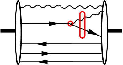
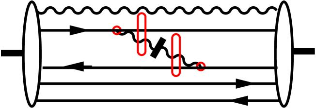
Figure 1: Regularization of the interaction by vertex regularization. In a matrix element, as illustrated on the left for a vertex, a quark changes its four-momentum from $k_{1}$ to $k_{2}$, i.e. $Q^{2}=-(k_{1}-k_{2})^{2}$. The vertex interaction is regulated by multiplying with a form factor $F(Q^{2})$, as indicated by the circle. – Instantaneous interactions are treated correspondingly, as illustration on the right for a seagull.

The light-cone wave functions $\Psi$ for a hadron with mass $M$ encode all possible quark and gluon momentum, helicity and flavor correlations and, in principle, are obtained by diagonalizing the QCD light-cone Hamiltonian $H_{\mathrm{LC}}=P^{+}P^{-}-P^{2}_{\!\perp}$, where $P^{\pm}=P^{0}\pm P^{z}$,

$$H_{\mathrm{LC}}|\Psi_{i}\rangle=M_{i}^{2}|\Psi_{i}\rangle$$ (7)

in a complete basis of Fock states with increasing complexity. For example, the positive pion has the Fock expansion:

$$|\Psi_{\pi^{+}}\rangle = \sum_{n}\langle n|\pi^{+}\rangle|n\rangle$$

$$= \Psi^{(\Lambda)}_{u\bar{d}/\pi}(x_{i},\vec{k}_{\!\perp i})|u\bar{d}\rangle+\Psi^{(\Lambda)}_{u\bar{d}g/\pi}(x_{i},\vec{k}_{\!\perp i})|u\bar{d}g\rangle+\dots\;,$$

representing the expansion of the exact QCD eigenstate at scale $\Lambda$ in terms of non-interacting quarks and gluons. The $i_{n}$ particles in a Fock state ($n$) have longitudinal light-cone momentum fractions $x_{i}$ and relative transverse momenta $\vec{k}_{\!\perp i}$, with

$$x_{i}=\frac{k_{i}^{+}}{P^{+}}=\frac{k_{i}^{0}+k_{i}^{z}}{P^{0}+P^{z}}\;,\quad\sum_{i=1}^{i_{n}}x_{i}=1\;,\quad\sum_{i=1}^{i_{n}}\vec{k}_{\!\perp i}=\vec{0}_{\!\perp}\;.$$

The form of $\Psi_{n/H}(x_{i},\vec{k}_{\!\perp i})$ is invariant under longitudinal and transverse boosts; i.e., the light-cone wave functions expressed in the relative coordinates $x_{i}$ and $k_{\!\perp i}$ are independent of the total momentum ($P^{+}$, $\vec{P}_{\!\perp}$) of the hadron. The first term in the expansion is referred to as the valence Fock state, as it relates to the hadronic description in the constituent quark model. The higher terms are related to the sea components of the hadronic structure. It has been shown that the rest of the light-cone wave function is determined once the valence Fock state is known Mue94 ; Pau99b , with explicit expressions given in Pau99b .

The key issue is to overcome the problem of any gauge theory, that the unregulated theory exposes logarithmic singularities. The problem of regularization and renormalization has been solved in the perturbative context of scattering theory, but not in the non perturbative context of a Hamiltonian. It is addressed to in the first two sections and applied in the remainder of this paper.

2 Regularization

Canonical field theory with the conventional QCD Lagrangian allows to derive the components of the total canonical four-momentum $P^{\mu}$. Its front form version BroPauPin98 rests on two assumptions, the light cone gauge $A^{+}=0$ LepBro80 and the suppression of all zero modes BroPauPin98 ; Kal95 . The front form vacuum is then trivial.

I find it helpful to discuss the problem in terms of DLCQ PauBro85a ; BroPauPin98 . In the back of my mind I visualize an explicit finite dimensional matrix representation of the Light-Cone Hamiltonian as it occurs for finite harmonic resolution. Such one is schematically displayed in Fig. 2 of BroPauPin98 . All of its matrix elements are finite for any finite $x$ and $k_{\!\perp}$.

The problem arises for ever increasing harmonic resolution, on the way to the continuum limit: The numerical eigenvalues are numerically unstable and diverge logarithmically KraPauWoe92 ; TriPau00 , contrary to the calculations in 1+1 dimension PauBro85a ; see also actual DLCQ calculations in 3+1 by Hiller Hil00 .

The reason is inherent to Dirac’s relativistic vertex interaction $\langle k_{1},h_{1}|V|k_{2},h_{2};k_{3},h_{3}\rangle$, in which some particle ‘1’ is scattered into two particles ‘2’ and ‘3’ with their respective four-momenta $k$ and helicities $h$, see Fig. 1. The matrix element for bremsstrahlung, for example, is proportional to $k_{\!\perp}$, $\langle k_{1},\uparrow|V|k_{2},\uparrow;k_{1},\uparrow\rangle\propto|\vec{k}_{\!\perp}|$, see Table 9 in BroPauPin98 , when the quark maintains its helicity while irradiating a gluon with four-momentum $k_{3}^{\mu}=(xP^{+},\vec{k}_{\!\perp},k_{3}^{-})$. Singularities arise typically when squares of such matrix elements are integrated over all $\vec{k}_{\!\perp}$ as in the integrations of perturbation theory.

The singularities are avoided a priori by vertex regularization, by multiplying each (typically off-diagonal) matrix element with a regulating form factor $F$:

$$\langle k_{1},h_{1}|V|k_{2},h_{2};k_{3},h_{3}\rangle\;\Longrightarrow$$

$$\langle k_{1},h_{1}|V|k_{2},h_{2};k_{3},h_{3}\rangle\;F(Q)\;.$$ (8)

It took several years to realize that it is the Feynman four-momentum transfer across a vertex, $Q^{2}=-(k_{1}-k_{2})^{2}$, which governs any effective interaction. The minimal requirement for such a form factor is

$$F(Q;\Lambda)=\left\{\begin{array}[]{ll}1\;,&\mbox{ for }Q^{2}\rightarrow 0\;,\\ 0\;,&\mbox{ for }Q^{2}\rightarrow\infty\;.\end{array}\right.$$ (9)

The job would be done by a step function, $F(Q)=\Theta(Q^{2}-\Lambda^{2})$. The limit $\Lambda\rightarrow 0$ suppresses the interaction all together, the limit $\Lambda\rightarrow\infty$ restores the interaction and its problems. Any finite value of $\Lambda^{2}$ restricts $Q^{2}$ to be finite and eliminates the singularities. But the sharp cut-off generates problems in an other corner of the theory and $F(Q)$ must be an analytic function of $Q$, as to be seen below.

Vertex regularization takes thus care of the ultraviolet divergences. The (light-cone) infrared singularities are taken care of as usual by a kinematical gluon mass.

As usual, regularization is not unique and many ways can do that. Dimensional regularization, for example, is not applicable in a matrix approach which is stuck with the precisely 3+1 dimensions of the physical world. Vertex regularization should be confronted with the Fock space regularization of Lepage and Brodsky LepBro80 , see also BroPauPin98 , which has blocked the renormalization aspects for many years. It also should be confronted with wil89 and WilWalHar94 . After applauding the light-cone approach wil89 , Wilson and collaborators WilWalHar94 have attempted to base their considerations almost entirely on a renormalization group analysis, but no concrete technology has emerged thus far.

3 Renormalization

The non perturbative renormalization of the Hamiltonian was stuck for many years by the fact that the coupling constant $g$ and the regulator function $F(Q)$ multiply each other in Eq.(8). It was always clear that one may add non local counter terms WilWalHar94 , but is was not clear how they could be constructed. Progress has come from recent work on a particular model FrewerFrePau02 , which did allow to formulate a paradigmatic example in modern renormalization theory.

Here is the general but abstract procedure.

Suppose to have solved Eq.(7) for a fixed value of the 7 ‘bare’ parameters in the Lagrangian, for the coupling constant $g=g_{0}$ and the 6 flavor quark masses $m_{f}=(m_{f})_{0}$, and for a fixed value of exterior cut-off scale $\Lambda=\Lambda_{0}$. Suppose further that these 7+1 parameters are chosen such, that the calculated $M^{2}_{i}$ agree with the corresponding experimental values. Next, suppose to change the cut-off by a small amount $\delta\Lambda$. Every calculated eigenvalue will then change by $\delta M^{2}_{i}$. Renormalization theory is then the attempt to reformulate the Hamiltonian, such, that all changes $\delta M^{2}_{i}$ vanish identically.

The fundamental renormalization group equation is therefore:

$$\left.dM^{2}_{i}\right|_{0}=\left.dM^{2}_{i}\right|_{g=g_{0},m_{f}=m_{f_{0}},\Lambda=\Lambda_{0}}=0\;,$$ (10)

for all eigenstates $i$. Equivalently one requires that the Hamiltonian is stationary with respect to small $\delta\Lambda$:

$$\left.\phantom{M^{2}_{i}}\delta H_{\mathrm{LC}}\right|_{0}=0\;.$$ (11)

Hence forward reference to ($g_{0},m_{f_{0}},\Lambda_{0}$), to the ‘renormalization point’, will be suppressed.

The Hamiltonian can be made stationary by making $g$ and the $m_{f}$ functions of $\Lambda$, by introducing physical coupling constants and masses, $\overline{g}$ and $\overline{m}_{f}$, respectively, which themselves are functions of the bare $g$ and $m_{f}$, and which are functionals of the regulator $\overline{F}=F$. The variation of $H_{\mathrm{LC}}$ reads then

$$\delta H_{\mathrm{LC}}=\delta\overline{g}\frac{\delta H_{\mathrm{LC}}}{\delta\overline{\alpha}}+\sum_{f}\delta\overline{m}_{f}\frac{\delta H_{\mathrm{LC}}}{\delta\overline{m}_{f}}+\delta\overline{F}\frac{\delta H_{\mathrm{LC}}}{\delta\overline{F}}=0\;,$$

with the familiar variational derivatives. However, since $\overline{g}$ and $\overline{m}_{f}$ are themselves functionals of $\overline{F}$, this reduces to

$$\delta H_{\mathrm{LC}}=\delta\overline{F}\frac{\delta H_{\mathrm{LC}}}{\delta\overline{F}}=0\;.$$

Eq.(10) as the fundamental equation of renormalization theory is then replaced by

$$\delta\overline{F}=\delta\Lambda\frac{\partial\overline{F}}{\partial\Lambda}=0\;,$$ (12)

since the variational derivative of the Hamiltionian with respect to the regulator is unlikely to vanish.

It can be solved by counter term technology, as follows. A counter term is added to the Hamiltonian, whose interaction has exactly the same structure except that the regulator $F(Q)$ is replaced by $C(Q)$. This defines

$$\overline{F}(Q,\Lambda)=F(Q,\Lambda)+C(Q,\Lambda)\;,$$ (13)

subject to the constraint that the counter term vanishes at the renormalization point,

$$\left.\phantom{\frac{d\overline{R}}{d\Lambda}}C(Q,\Lambda)\right|_{\Lambda=\Lambda_{0}}=0\;.$$ (14)

The fundamental equation (12) defines then a differential equation

$$\frac{dC(Q;\Lambda)}{d\Lambda}=-\frac{dF(Q;\Lambda)}{d\Lambda}\;,$$ (15)

which, in its integral form, includes the initial condition

$$C(Q,\Lambda)=-\int\limits_{\Lambda_{0}}^{\Lambda}\!\!ds\ \frac{dF(Q,s)}{ds}=F(Q,\Lambda_{0})-F(Q,\Lambda)\;.$$ (16)

The renormalized regulator function, $\overline{F}=F+C$,

$$\overline{F}(Q,\Lambda)=F(Q,\Lambda_{0})\;,$$ (17)

is manifestly independent of $\Lambda$. By construction, the value of $\Lambda_{0}$ is determined by experiment.

One should emphasize an important point: In deriving Eq.(17), use was made of assuming the regulator function has well defined derivatives with respect to $\Lambda$. The theta function of the sharp cut-off, however, is a distribution with only ill defined derivatives.

This raises an other important point: If $F(Q,\Lambda)$ is a function of $Q/\Lambda$ other than a theta function, one must specify how the function approaches the limiting values of Eq.(9). The case of the ‘soft’ regulator

$$F(Q,\Lambda)=\frac{\Lambda^{2}}{\Lambda^{2}+Q^{2}}$$ (18)

is only a very special example. In a more general approach the soft regulator plays the role of a generating function

$$F(Q,\Lambda)=\left[1+\sum_{n=1}^{N}(-1)^{n}s_{n}\Lambda^{n}\frac{\partial^{n}}{\partial\Lambda^{n}}\right]\frac{\Lambda^{2}}{\Lambda^{2}+Q^{2}}\;.$$ (19)

The partials $\Lambda^{n}\,\partial^{n}/\partial\Lambda^{n}$ are dimensionless and independent of a change in $\Lambda$. The arbitrarily many coefficients $s_{1},\dots,s_{N}$ are renormalization group invariants and, as such, subject to be determined by experiment.

4 The effective (light-cone) Hamiltonian

In a field theory, one is confronted with a many-body problem of the worst kind: Not even the particle number is conserved. For to formulate effective Hamiltonians more systematically, a novel many-body technique had to be developed, the method of iterated resolvents Pau99b ; Pau98 , whose details are not important here.

Important is that the effective light-cone Hamiltonian $H_{\mathrm{eLC}}$ has the same eigenvalue as the full light-cone Hamiltonian $H_{\mathrm{LC}}$ and that it generates the bound state wave function of valence quarks by an one-body integral equation in ($x,\vec{k}_{\!\perp}$):

$$M^{2}\psi_{h_{1}h_{2}}(x,\vec{k}_{\!\perp})=\left[\frac{\overline{m}^{2}_{1}+\vec{k}_{\!\perp}^{\,2}}{x}+\frac{\overline{m}^{2}_{2}+\vec{k}_{\!\perp}^{\,2}}{1-x}\right]\psi_{h_{1}h_{2}}(x,\vec{k}_{\!\perp})$$ (20)

$$- {1\over 3\pi^{2}}\sum_{h_{q}^{\prime},h_{\bar{q}}^{\prime}}\!\int\!\frac{dx^{\prime}d^{2}\vec{k}_{\!\perp}^{\prime}}{\sqrt{x(1-x)x^{\prime}(1-x^{\prime})}}\;\psi_{h_{1}^{\prime}h_{2}^{\prime}}(x^{\prime},\vec{k}_{\!\perp}^{\prime})$$

$$\times F(Q_{q})F(Q_{\bar{q}})\left(\frac{\overline{\alpha}(Q_{q})}{2Q_{q}^{2}}+\frac{\overline{\alpha}(Q_{\bar{q}})}{2Q_{\bar{q}}^{2}}\right)$$

$$\times \left[\overline{u}(k_{1},h_{1})\gamma^{\mu}u(k_{1}^{\prime},h_{2}^{\prime})\right]\left[\overline{v}(k_{2}^{\prime},h_{2}^{\prime})\gamma_{\mu}v(k_{2},h_{2})\right]\;.$$

One has achieved step 2 of Eq.(6): $H_{\mathrm{eLC}}|\Psi_{q\bar{q}}\rangle=M^{2}|\Psi_{q\bar{q}}\rangle$. Here, $M^{2}$ is the eigenvalue of the invariant-mass squared. The associated eigenfunction $\psi_{h_{1}h_{2}}(x,\vec{k}_{\!\perp})$ is the probability amplitude $\langle x,\vec{k}_{\!\perp},h_{1};1-x,-\vec{k}_{\!\perp},h_{2}|\Psi_{q\bar{q}}\rangle$ for finding the quark with momentum fraction $x$, transversal momentum $\vec{k}_{\!\perp}$ and helicity $h_{1}$, and correspondingly the anti-quark. Expressions for the (effective) quark masses $\overline{m}_{1}$ and $\overline{m}_{2}$ and the (effective) coupling function $\overline{\alpha}(Q)$ are given in Pau98 . $Q_{q}$ and $Q_{\bar{q}}$ are the Feynman momentum transfers of quark and anti-quark, respectively, and $u(k_{1},h_{1})$ and $v(k_{2},h_{2})$ are their Dirac spinors in Lepage Brodsky convention LepBro80 , given explicitly in BroPauPin98 . They arrange themselves in the Lorenz scalar spinor matrix

$$\langle h_{1},h_{2}|S|h_{1}^{\prime},h_{2}^{\prime}\rangle = \left[\overline{u}(k_{1},h_{1})\gamma^{\mu}u(k_{1}^{\prime},h_{1}^{\prime})\right]$$

$$\times \left[\overline{v}(k_{2}^{\prime},h_{2}^{\prime})\gamma_{\mu}v(k_{2},h_{2})\right]\,$$

which is a rather complicated (matrix) function of its six arguments $x,x^{\prime},\vec{k}_{\!\perp},\vec{k}_{\!\perp}^{\prime}$, as tabulated in Pau00c . Finally, the form factors $F(Q)$ restrict the range of integration and regulate the interaction. Note that the equation is fully relativistic and covariant.

It should be emphasized that Eq.(20) is valid only for quark and anti-quark having different flavors Pau99b ; Pau98 . The additional annihilation term for identical flavors is omitted. At present, it is investigated by Kra04 . It should also be emphasized that the same structure was obtained with a completely different method, with Wegner’s Hamiltonian flow equations Wegner00 . In Wegner00 is also shown why the concept of a ‘mean momentum transfer’, $Q^{2}=\frac{1}{2}\left(Q_{q}^{2}+Q_{\bar{q}}^{2}\right)$ is a meaningful simplification. It allows to replace Eq.(20) by

$$M^{2}\psi_{h_{1}h_{2}}(x,\vec{k}_{\!\perp})=\left[\frac{\overline{m}^{2}_{1}+\vec{k}_{\!\perp}^{\,2}}{x}+\frac{\overline{m}^{2}_{2}+\vec{k}_{\!\perp}^{\,2}}{1-x}\right]\psi_{h_{1}h_{2}}(x,\vec{k}_{\!\perp})$$ (21)

$$- {1\over 3\pi^{2}}\sum_{h_{q}^{\prime},h_{\bar{q}}^{\prime}}\!\int\!\displaystyle\frac{dx^{\prime}d^{2}\vec{k}_{\!\perp}^{\prime}\;\psi_{h_{1}^{\prime}h_{2}^{\prime}}(x^{\prime},\vec{k}_{\!\perp}^{\prime})}{\sqrt{x(1-x)x^{\prime}(1-x^{\prime})}}\frac{\overline{\alpha}(Q)}{Q^{2}}\overline{R}(Q)$$

$$\times \left[\overline{u}(k_{1},h_{1})\gamma^{\mu}u(k_{1}^{\prime},h_{2}^{\prime})\right]\left[\overline{v}(k_{2}^{\prime},h_{2}^{\prime})\gamma_{\mu}v(k_{2},h_{2})\right]\;.$$

The form factors $F(Q)$ have made their way into the regulator function $\overline{R}(Q)=F^{2}(Q)$. Krautgärtner et al KraPauWoe92 and Trittmann et al TriPau00 have shown how to solve numerically such an equation with a high precision. But since the numerical effort is so considerable, it is reasonable to work first with (over-)simplified models, as specified next.

The Singlet-Triplet model. Quarks are at relative rest when $\vec{k}_{\!\perp}=0$ and $x=\overline{x}$, with $\overline{x}\equiv\overline{m}_{1}/(\overline{m}_{1}+\overline{m}_{2})$. An inspection of Eq.(33) in Pau00c reveals that for very small deviations from the equilibrium values, the spinor matrix $\langle h_{1},h_{2}|S|h_{1}^{\prime},h_{2}^{\prime}\rangle$ is proportional to the unit matrix,

$$\langle h_{1},h_{2}|S|h_{1}^{\prime}h_{2}^{\prime}\rangle \simeq 4\overline{m}_{1}\overline{m}_{2}\;\delta_{h_{1},h_{1}^{\prime}}\;\delta_{h_{2},h_{2}^{\prime}}\;.$$ (22)

For very large deviations, particularly for $\vec{k}_{\!\perp}^{\prime\,2}\gg\vec{k}_{\!\perp}^{\,2}$, holds

$$Q^{2}\simeq\vec{k}_{\!\perp}^{\prime\,2}\;,\quad\mbox{and}\quad\langle\uparrow\downarrow|S|\uparrow\downarrow\rangle\simeq 2\vec{k}_{\!\perp}^{\prime\,2}\;.$$ (23)

The Singlet-Triplet (ST) model combines these aspects:

$$\langle h_{1},h_{2}|S|h_{1}^{\prime},h_{2}^{\prime}\rangle = \delta_{h_{1},h_{1}^{\prime}}\;\delta_{h_{2},h_{2}^{\prime}}\;\langle h_{1},h_{2}|S|h_{1},h_{2}\rangle\;,$$ (24)

$$\frac{\langle h_{1},h_{2}|S|h_{1},h_{2}\rangle}{Q^{2}} = \left\{\begin{array}[]{ll}\frac{4\overline{m}_{1}\overline{m}_{2}}{Q^{2}}+2,&\mbox{ for $h_{1}=-h_{2}$,}\\ \frac{4\overline{m}_{1}\overline{m}_{2}}{Q^{2}},\phantom{+2}&\mbox{ for $h_{1}=\phantom{-}h_{2}$.}\\ \end{array}\right.$$ (27)

For anti parallel helicities $h_{1}=-h_{2}$ (singlets) the model interpolates between two extremes: For small momentum transfer $Q$, the ‘2’ in Eq.(23) is unimportant and the Coulomb aspects of the first term prevail. For large $Q$, the Coulomb aspects are unimportant and the hyperfine interaction is dominant. The ‘2’ carries the singlet triplet mass difference: Its value is understood by $g_{s}\left(\frac{1}{4}-\left(-\frac{3}{4}\right)\right)=g_{s}$, with the spin-g factor $g_{s}=2$. For parallel helicities $h_{1}=h_{2}$ (triplets) the model reduces to the Coulomb kernel. The model over emphasizes many aspects but its simplicity has proven useful for fast and analytical calculations. Most importantly, the model allows to drop the helicity summations which technically simplifies the problem enormously. A more detailed investigation of the spinor matrix can be found in KrassPau02 .

The model can not be justified in the sense of an approximation, but it emphasizes the point that the ‘2’, or any other constant in the kernel of an integral equation, leads to numerically undefined equations and thus singularities. Replacing the function $\overline{\alpha}(Q)$ by the strong coupling constant $\alpha_{s}=g^{2}/4\pi$ completes the model assumptions. Hence forward, the overline bars for the effective quantitites will be suppressed.

5 The potential energy

It is possible to subtract a c-number from $H_{\mathrm{eLC}}$ and to define an effective Hamiltonian $H_{\mathrm{eff}}$ implicitly by

$$H_{\mathrm{eLC}}\equiv\left(m_{1}+m_{2}\right)^{2}+2\left(m_{1}+m_{2}\right)H_{\mathrm{eff}}\;.$$ (28)

Its eigenvalues have the dimension of an energy

$$H_{\mathrm{eff}}|\varphi\rangle=E|\varphi\rangle\;,$$

achieving this way step 3 of Eq.(6). Note that mass and energy in the front form, on the light cone, are related by

$$\hskip 55.97205ptM^{2}=\left(m_{1}+m_{2}\right)^{2}+2\left(m_{1}+m_{2}\right)E\;,$$ (29)

and not by $\;M^{2}=\left(m_{1}+m_{2}\right)^{2}+2\left(m_{1}+m_{2}\right)E+E^{2}$, as usual. Only if the energy is negligible as compared to the quark masses, i.e. only if $\left(E/(m_{1}+m_{2})\right)^{2}\ll 1$, the two relations coincide.

A rather drastic technical simplification is achieved by a transformation of the integration variable. One can substitute the integration variable $x$ by the integration variable $k_{z}$, which, for all practical purposes, can be interpreted BroPauPin98 as the $z$-component of a 3-momentum vector $\vec{p}=(k_{z},\vec{k}_{\!\perp})$. For equal masses $m_{1}=m_{2}=m$, the transformation is, together with its inverse,

$$x(k_{z}) = \frac{1}{2}\left[1+\frac{k_{z}}{\sqrt{m^{2}+\vec{k}_{\!\perp}^{\;2}+k_{z}^{2}}}\right]\;.$$ (30)

$$k_{z}^{2}(x) = (m^{2}+\vec{k}_{\!\perp}^{\,2})\ \frac{\left(x-\frac{1}{2}\right)^{2}}{x(1-x)}\;.$$ (31)

Inserting these substitutions into Eq.(21) and defining the reduced wave function $\varphi$ by

$$\psi_{h_{1}h_{2}}(x,\vec{k}_{\!\perp}) = \frac{\sqrt{A(k_{z},\vec{k}_{\!\perp})}}{\sqrt{x(1-x)}}\varphi_{h_{1}h_{2}}(k_{z},\vec{k}_{\!\perp})\,,$$ (32)

$$A(\vec{p}) = \sqrt{1+\frac{\vec{p}^{\,2}}{m^{2}}}\;,$$ (33)

leads to an integral equation in the components of $\vec{p}$, in which all reference to light-cone variables has disappeared. Using in addition the ST-model of Eq.(24), Eq.(21) translates for singlets identically into

$$M^{2}\varphi(\vec{p})=4\left[m^{2}+\vec{p}^{2}\right]\varphi(\vec{p})$$

$$- \frac{\alpha_{c}}{2\pi^{2}}\int\!\frac{d^{3}p^{\prime}}{\sqrt{A(p)A(p^{\prime})}}\left(\frac{4m^{2}}{Q^{2}}+2\right)\frac{R(Q)}{m}\;\varphi(\vec{p}^{\prime})\;,$$

with $\alpha_{c}=\frac{4}{3}\alpha_{s}$. The equation for the triplets is obtained by dropping the ‘2’. In the ST-model, the helicity arguments in the wave functions can be suppressed. Applying the relation between mass and energy, as given in Eq.(29), the equation is converted to

$$E\varphi(\vec{p})=\frac{\vec{p}^{2}}{2m_{r}}\varphi(\vec{p})$$

$$- \frac{\alpha_{c}}{2\pi^{2}}\int\!\frac{d^{3}p^{\prime}}{\sqrt{A(p)A(p^{\prime})}}\left(\frac{4m^{2}}{Q^{2}}+2\right)\frac{R(Q)}{4m^{2}}\;\varphi(\vec{p}^{\prime})\;,$$

since the reduced mass for $m_{1}=m_{2}=m$ is $m_{r}=m/2$.

The first term in this equation, $\vec{p}^{2}/2m_{r}$, coincides with the kinetic energy in a conventional non-relativistic Hamiltonian. This is remarkable in view of the fact that no approximation to this extent has been made. The fully relativistic and covariant light-cone approach has no relativistic corrections in the kinetic energy!

Since the first term in Eq.(5) is a kinetic energy, the second must be a potential energy — in a momentum representation. In principle, it could be Fourier transformed with $\mathrm{e}^{-i\vec{p}\vec{r}}$ to a configuration space with the variable $\vec{r}$. But due to the factor $A(p)A(p^{\prime})$ in the kernel, the resulting potential energy would be non-local, see f.e. PauMer97 .

The non-locality of the potential is certainly mathematically exact. But I do not expect this to generate aspects of leading importance, and avoid it by the simplification $A(p)\equiv 1$, both in Eqs.(32) and (5).

With $A(p)=1$, the mean four momentum transfer $Q^{2}$ reduces to the three momentum transfer $q^{2}=(\vec{p}-\vec{p}^{\prime})^{2}$. In consequence, the kernel of Eq.(5),

$$U(\vec{q}) = -\frac{\alpha}{2\pi^{2}}\left(\frac{4m^{2}}{q^{2}}+2\right)\frac{R(q)}{4m^{2}}\;,$$ (36)

depends only on $\vec{q}=\vec{p}-\vec{p}^{\prime}$. Its Fourier transform is a local function,

$$V(\vec{r}) = \int\!d^{3}q\;\mathrm{e}^{-i\vec{q}\vec{r}}\;U(\vec{q})\;,$$ (37)

which plays the role of a conventional potential energy in the Fourier transform of Eq.(5), i.e. in

$$E\;\psi(\vec{r}) = \left[\frac{\vec{p}^{2}}{2m_{r}}+V(\vec{r})\right]\psi(\vec{r})\;.$$ (38)

Here is the Schrödinger equation from Eq.(6) ! Despite its conventional structure it is a front form equation, designed to calculate the light-cone wave function $\psi(\vec{r})\rightarrow\varphi(\vec{p})\rightarrow\psi_{q\bar{q}}(x,\vec{k}_{\!\perp})$.

I conclude this section with a subtle point, which needs clarification in the future. The simplification $A(p)=1$ is different from a non-relativistic approximation. The approach is certainly valid also for relativistic momenta $p^{2}\gg m^{2}$, particularly Eqs.(5) and (37). The reason is that $A(p)$ occurs only under the integral. There, the large momenta are suppressed by the regulator, anyway.

6 The renormalized Coulomb potential

Hence forward, I restrict consideration to the triplet case, i.e. to Coulomb kernels like $U(\vec{q})\sim R(q)/q^{2}$. The renormalized Coulomb potential is always finite at the origin, as opposed to the conventional $\frac{1}{r}$–singularity. It is instructive to verify this explicitly for two regulators:

$$U(q)=\left\{\begin{array}[]{ll}-\frac{\alpha_{c}}{2\pi^{2}q^{2}}\;\frac{\lambda^{2}}{q^{2}+\lambda^{2}},&\mbox{for the soft cut-off},\\ -\frac{\alpha_{c}}{2\pi^{2}q^{2}}\;\Theta(q^{2}-\lambda^{2}),&\mbox{for the sharp cut-off}.\end{array}\right.$$ (41)

The Fourier transform according to Eq.(36) gives

$$V(r)=\left\{\begin{array}[]{ll}-\frac{\alpha_{c}}{r}\;(1-\mathrm{e}^{-\lambda r}),&\mbox{for the soft cut-off},\\ -\frac{\alpha_{c}}{r}\;\frac{2}{\pi}\mathrm{Si}(\lambda r),&\mbox{for the sharp cut-off},\end{array}\right.$$ (44)

where $\mathrm{Si}$ is the Integral Sine. Asymptotically holds:

$$\lim_{r\rightarrow\infty}V(r)=\left\{\begin{array}[]{ll}-\frac{\alpha_{c}}{r},&\mbox{for the soft cut-off},\\ -\frac{\alpha_{c}}{r},&\mbox{for the sharp cut-off}.\end{array}\right.$$ (47)

Both cut-offs produce the conventional Coulomb potential. Near the origin, however, holds:

$$\lim_{r\rightarrow 0}V(r) = \alpha_{c}\lambda\cdot\left\{\begin{array}[]{ll}-1+\frac{(\lambda r)\phantom{{}^{2}}}{2},&\mbox{for the soft cut-off},\\ -\frac{2}{\pi}+\frac{(\lambda r)^{2}}{9\pi},&\mbox{for the sharp cut-off}.\end{array}\right.$$ (50)

The renormalized Coulomb potential is finite but the constant is cut-off dependent. Even the $r$-dependence differs: The soft cut-off gives a linear and the sharp cut-off a quadratic dependence.

The cut-off dependence near the origin is one of the most important aspects of the present work and has a deep physical reason to be discussed below. Recalling the discussion in Sec. 3 and replacing the soft cut-off in analogy to Eq.(19) with

$$R(q)=\left[1+\sum_{n=1}^{N}(-1)^{n}s_{n}\lambda^{n}\frac{\partial^{n}}{\partial\lambda^{n}}\right]\frac{\lambda^{2}}{\lambda^{2}+q^{2}}\;,$$ (51)

gives straightforwardly the generalized Coulomb potential

$$V(r) = -\frac{\alpha_{c}}{r}\Big{[}1+\sum_{n=1}^{N}(-1)^{n}s_{n}\lambda^{n}\frac{\partial^{n}}{\partial\lambda^{n}}\Big{]}\Big{(}1-\mathrm{e}^{-\lambda r}\Big{)}$$ (52)

$$= \phantom{-}\frac{\alpha_{c}}{r}\Big{[}-1+\mathrm{e}^{-{\lambda r}}\sum_{n=0}^{N}s_{n}({r\lambda})^{n}\Big{]},$$

with $s_{0}\equiv 1$. This result illustrates an other important point: The Laguerre polynomials are a complete set of functions. The term added to the -1 in Eq.(52) is thus potentially able to reproduce an arbitrary function of $r$. The description in terms of a generating function, as in Eqs.(51) or (52), is therefore complete.

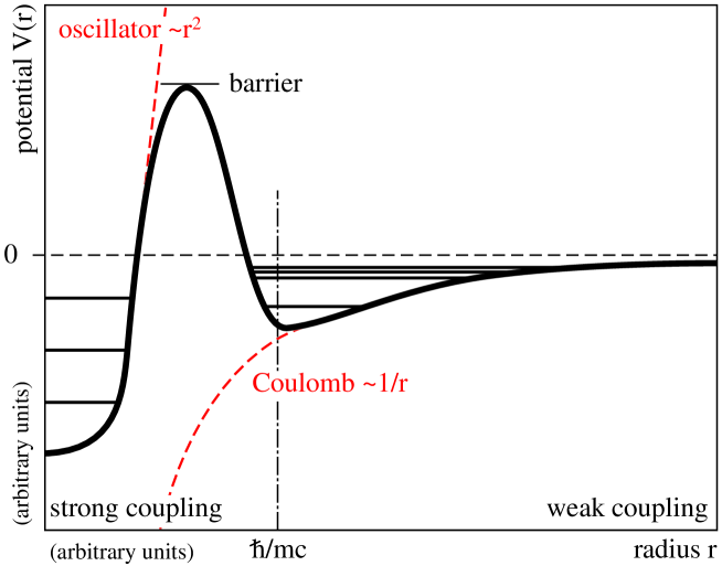
Figure 2: Schematic behavior of the renormalized Coulomb potential, see also the discussion in the text.

The physical picture which develops is illustrated in Fig. 2. In the far zone, for sufficiently large $r$, the potential energy coincides with the conventional Coulomb potential $-\frac{\alpha_{c}}{r}$. Since the potential is attractive, it can host bound states which are probably those realized in weak binding. In the near zone, for sufficiently small $r$, the potential behaves like a power series $c_{0}+c_{1}r+c_{2}r^{2}$ which potentially can host the bound states of strong coupling, provided the actual parameter values allow for that. In the intermediate zone, the actual potential must interpolate between these two extremes, since Eq.(52) is an analytic function of $r$. Most likely this is done by developing a barrier of finite height, depending on the actual parameter values. The onset of the near and intermediate regimes must occur for relative distances of the quarks, which are comparable to the Compton wave length associated with their reduced mass. If the distance is smaller, one expects deviations from the classical regime by elementary considerations on quantum mechanics, indeed.

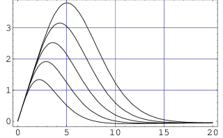
Figure 3: The dimensionless Coulomb potential $W_{N}(y;0,1,0)$ is plotted versus the radius parameter $y=\lambda r$ for different $N$, i.e. from bottom to top for $N=4,5,6,7,8$.

The large number of parameter in Eq.(52) can be controlled by the following construction: The coefficients $s_{n}$ in Eq.(52) are expressed in terms of only three parameters $a$, $b$, and $c$, by

$$s_{n}=\frac{1}{n!}+\frac{a}{(n-1)!}+\frac{b}{(n-2)!}+\frac{c}{(n-3)!}\,.$$ (53)

The first few coefficients are then explicitly

$$\begin{array}[]{rc rc rc rc rc rc }s_{0}&=&1&,&\\ s_{1}&=&1&+&a&,&\\ s_{2}&=&\frac{1}{2}&+&a&+&b&,&\\ s_{3}&=&\frac{1}{6}&+&\frac{a}{2}&+&b&+&c&,&\\ s_{4}&=&\frac{1}{24}&+&\frac{a}{6}&+&\frac{b}{2}&+&c&.&\end{array}$$ (59)

As a consequence, the dimensionless Coulomb potential,

$$W_{N}(y;a,b,c)=\frac{V(r)}{\alpha_{c}\lambda}=\frac{1}{y}\Big{(}-1+\mathrm{e}^{-y}\sum_{n=0}^{N}s_{n}y^{n}\Big{)}\,,$$ (60)

which depends on $r$ only through the dimensionless combination $y=\lambda r$, is at most a quadratic function of $y$,

$$W_{N}(y;a,b,c)=a+by+cy^{2}\,,$$ (61)

in the near zone, and thus independent of $N$. The remainder starts at most with power $y^{N+1}$. A value of $a=c=0$ and $b=1$ should therefore yield a linear set of functions $W_{N}(y;a,b,c)=y$ in the near zone. As shown in Fig. 3 this happens to be true for surprisingly large values of $y$, i.e. not only for $y\ll 1$. The value of $N$ essentially controls the height of the barrier. Similarly, $W_{N}(y;0,0,1)=y^{2}$ generates a set of functions which are strictly quadratic in the near zone. Again, $N$ controls the height of the barrier, as to be seen below in Fig. 5.

7 Determining the parameters by experiment

The QCD-inspired model developed thus far has a considerable number of renormalization group invariant parameters, which must be determined once and for all by experiment.

In doing this FrePauZho02b , we have been inspired by the work of Anisovich et al. AniAniSar02 . Enumerating the excited states of a hadron by a counting index $n=0,1,2,\dots$, these authors have found the linear relation $M_{n}^{2}=M_{0}^{2}+n\chi$ for practically all hadrons. As an example, I present in Fig. 4 the spectrum of the $\pi$- and the $\rho$-meson.

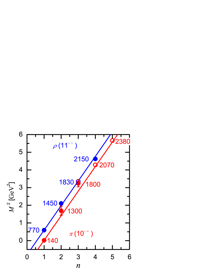
Figure 4: The invariant mass-squares of all available $\pi^{+}$– and $\rho^{+}$–states are plotted versus a counting index $n=0,1,2,\dots$. The straight lines correspond to $M_{n}^{2}=M_{0}^{2}+n\chi$, with the value $\chi=1.39\mbox{ GeV}^{2}$, taken from Anisovich et al. AniAniSar02 . The filled circles correspond to states which have been seen empirically PDG98 , the empty ones correspond to the predictions AniAniSar02 . — Plot courtesy of Shan-Gui Zhou.

The linear relation between mass–squared and energy on the light cone, Eq.(29), allows then to conclude that the potential energy in the near zone must be a pure oscillator,

$$V(r) = -c_{t}+\frac{1}{2}f_{t}r^{2}\;,$$ (62)

at least to first approximation, and that $b=0$ in Eq.(61). If one addresses to reproduce the spectra of all flavor off-diagonal triplet mesons (pseudo-vector mesons), except the topped ones, one has to determine 6 parameters: The 2 constants from the oscillator model, $c_{t}$ and $f_{t}$, and the 4 effective flavor quark masses $m_{u}=m_{d}$, $m_{s}$, $m_{c}$, and $m_{b}$. To determine them, one needs 6 experimental numbers, and I take from PDG98 :

$$\begin{array}[]{r@{}c@{}l r@{}c@{}l r@{}c@{}l}M_{u\bar{d},t0}&=&0.768,&M_{u\bar{s},t0}&=&0.892,&M_{u\bar{c},t0}&=&2.010,\\ M_{u\bar{d},t1}&=&1.465,&M_{u\bar{s},t1}&=&1.680,&M_{u\bar{b},t0}&=&5.325,\end{array}$$ (65)

all in GeV. The notation should be self-explanatory. For example, $M_{u\bar{d},t1}$ refers to the first excited state of the $\rho^{+}$. The so obtained parameter values are:

$$\begin{array}[]{|@{\ }c@{\ }|@{\ }c@{\ }|@{\ }c@{\ }|@{\ }c@{\ }||@{\ }c@{\ }|@{\ }c|}\hline\cr m_{u}&m_{s}&m_{c}&m_{b}&c_{t}&f_{t}\\ 0.218&0.438&1.749&5.068&0.880&0.0869\\ \mathrm{GeV}&\mathrm{GeV}&\mathrm{GeV}&\mathrm{GeV}&\mathrm{GeV}&\mathrm{GeV}^{3}\\ \hline\cr\end{array}$$ (69)

The numbers differ slightly from those in FrePauZho02b , due to choosing the empirical data set different from Eq.(65), but yield about the same overall agreement with all available experimental states of pseudo-vector mesons.

Reverting the argument, one concludes as in FrePauZho02b that the oscillator model in Eq.(62) explains quite naturally the systematics found by Anisovich et al. AniAniSar02 . But one can do even better.

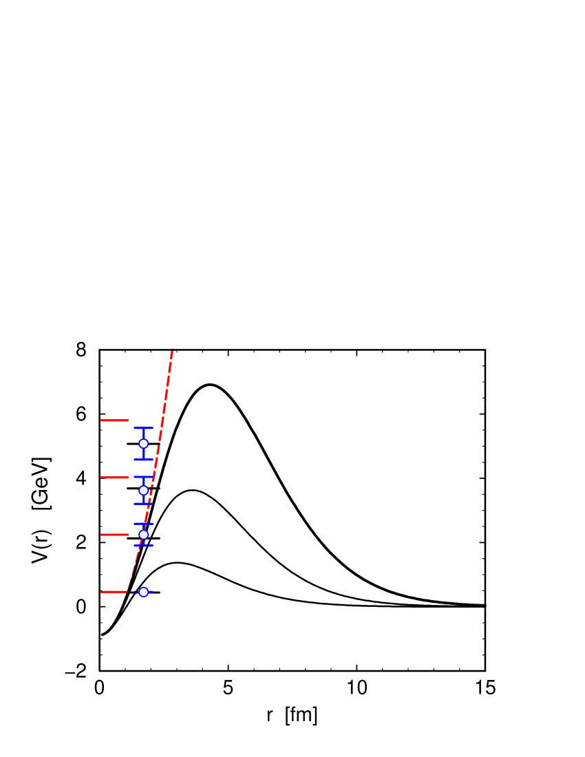
Figure 5: The continuous lines display the generalized Coulomb potential $V(r)=\alpha_{c}\lambda W_{N}(\lambda r;a,0,c)$ in physical units as function of $r$, for the values $N=4,5,6$ from bottom to top. The circles indicate the experimental eigenvalues $E_{n}$ for the $\rho^{+}$. They agree with the calculated eigenvalues for $N=6$, shown by the horizontal lines. — The dashed line displays the harmonic approximation; the horizontal lines on the left indicate the oscillator states. — See the discussion in the text.

8 Relating the oscillator model to QCD

The oscillator model in Eq.(62) is only the harmonic approximation to the QCD–inspired, generalized Coulomb potential in Eq.(52). Their parameters are related obviously by

$$c_{t} = -\alpha_{c}\lambda a\,,\qquad b=0\,,\qquad f_{t}=2\alpha_{c}\lambda^{3}c\;.$$ (70)

One needs more experimental information to pin down the value of $a$, $c$ and $N$. Choosing $\lambda$ as the QCD scale, i.e.

$$\lambda = 200\mbox{ MeV}\;,$$ (71)

one can use the expressions for $\overline{\alpha}(Q)$ in Pau98 to calculate $\alpha_{s}\equiv\overline{\alpha}(0)$ from the measured value of the coupling constant at the $Z$-mass $M_{Z}=91.2\mbox{ GeV}$,

$$\overline{\alpha}(M_{Z}) = 0.118\,,\quad\mbox{ thus }\quad\alpha_{s}\equiv\overline{\alpha}(0)=0.1695\;,$$ (72)

as to be shown in greater detail in Pau03b . Having fixed $\alpha_{c}=\frac{4}{3}\alpha_{s}$ and $\lambda$ allows to calculate $a$ and $c$ from $c_{t}$ and $f_{t}$, i.e.

$$a = -19.5\,,\qquad c=24.0\;.$$ (73)

We are thus able to draw the generalized Coulomb potential $V(r)=\alpha_{c}\lambda W_{N}(\lambda r;a,0,c)$ for different $N$ as done in Fig. 5. The ‘experimental’ eigenvalues $E_{0}$—$E_{3}$ for the $\rho$–meson, obtained by means of $E_{n}=(M_{n}^{2}-4m_{u}^{2})/(4m_{u})$, see Eq.(29), are also inserted, including the empirical limits of error. The experimental error $\delta E_{\rho,3}\sim\pm 0.5$ GeV (thus $\delta M_{\rho,3}\sim\pm 0.1$ GeV) is hypothetical, since $M_{\rho,3}$ is not confirmed. Taking it for granted, the lowest possible value for $N$ is thus

$$N=6\;.$$ (74)

This completes the determination of all parameters. They are universal within the model. I thank Harun OmerOme04 for giving me the exact eigenvalues prior to publication.

9 Summary and Conclusions

This work is an important mile stone on the long way from the canonical Lagrangian for quantum chromo dynamics down to the composition of physical hadrons in terms of their constituting quarks and gluons, by the eigenfunctions of a Hamiltonian.

As part of a on-going effort, a denumerable number of simplifying assumptions had to be phrased for getting a manageable formalism Pau99b . Among them is the formulation of an effective interaction by the method of iterated resolvents Pau98 , but the strongest assumption in the present work is probably the simplifying Singlet-Triplet model in Sec. 4. As long as the assumption are not proven at least a posteriori, one must speak of an approach inspired by QCD. It is advantageous, however, to have a sufficiently simple formalism for penetrating the physical content of gauge theory by analytical relations.

The biggest progress of the present work can be found in Sects. 2 and 3. It is related to a consistent regularization and renormalization of a gauge theory. The ultraviolet divergences in gauge theory are caused less by the possibly large momenta of the constituent particles, but by the large momentum transfers in the interaction. In a Hamiltonian approach, such as the present, one has not much choice else than to chop them off by a regulating form factor in the elementary vertex interaction.

The form factor makes its way into a regulator function which suppresses the large momentum transfers in the Fourier transform of the Coulomb interaction, see Sec. 6. The arbitrariness in chopping off the large momentum transfers is reflected in the arbitrariness of the potential at small relative distances. It is this arbitrariness which allows for a pocket in the potential which binds the quarks in a hadron.

The problem is then how to fix this function with its many parameters, by experiment. In practice this is less difficult than anti-cipated, see Sec. 7. It suffices to determine only three parameters, two continuous ones and one counting index.

The potential energy of the present work vanishes at an infinite separation of the quarks. This seems be be in conflict with the potential energies of phenomenological models GodIsg85 which rise forever. It also seems to be in conflict with lattice gauge calculations Schilling2000 ; Schierholz00 . Is a finite ionization limit in conflict also with ‘confinement’, i.e. with the empirical fact that free quarks have not been observed? — The present model prohibits free quarks as a stable solution, since the sum of the constituent quark masses is always larger than the mass of the corresponding hadron and a pion. Free constituent quarks would hadronize very quickly into bound states. This is different from atomic physics with its free constituents, where the binding energy is always much smaller than the mass of positronium proper.

The most disturbing aspect of the present work is its obvious conflict with lattice gauge calculations Schilling2000 ; Schierholz00 and their successes. Several points however should be made: I have not checked to which extent a linear term in the potential is consistent with the excellent agreement between theory and experiment presented in this work. – Even with present day computers lattice gauge calculations can be extrapolated down to such light systems as the $\pi$ or the $\rho$ only with a head ake. – The calculation of the potential energy on the lattice rests on the assumptions of static quarks, of quarks with an infinitely large mass. Whether this object is the potential energy to be used in a non relativistic Hamiltonian is an open question, as well as whether its eigenvalue can simply be added to the constituent masses to get the invariant mass of physical hadrons. In principle, the relation is justified only only for sufficiently small coupling constants.

The present work opens a broad avenue of further applications, among them also the baryons and physical nuclei. But much work must be done in the future before such a simple approach as the present must be taken serious. It is a first step only.

References

- (1) H.C. Pauli and S.J. Brodsky, Phys.Rev. D32 (1985) 1993.
- (2) P.A.M. Dirac, Rev. Mod. Phys. 21 (1949) 392.
- (3) S.J. Brodsky, H.C. Pauli, and S.S. Pinsky, Phys. Rep. 301 (1998) 299-486.
- (4) A.H. Mueller, Nucl. Phys. B415 (1994) 373.
- (5) H.C. Pauli, in: New directions in Quantum Chromodynamics, C.R. Ji and D.P. Min, Eds., American Institute of Physics, 1999, p. 80-139; hep-ph/9910203.
- (6) G.P. Lepage and S.J. Brodsky, Phys.Rev.D22 (1980) 2157.
- (7) A.C. Kalloniatis, Phys. Rev. D54 (1996) 2876.
- (8) J. Hiller, Nucl. Phys. B (Proc.Suppl.) 90 (2000) 170.
- (9) K. Wilson, in Lattice ’89, R. Petronzio, Ed., Nucl.Phys. B (Proc. Suppl.) 17 (1990) 82.
- (10) K.G. Wilson, T. Walhout, A. Harindranath, W.M. Zhang, R.J. Perry, and S.D. Glazek, Phys.Rev. D49 (1994) 6720.
- (11) H.C. Pauli, Compendium of Light-Cone Quantization, Nucl. Phys. B (Proc. Suppl.) 90 (2000) 259.
- (12) H.C. Pauli, Eur. Phys. J. C7 (1998) 289.
- (13) H.C. Krahl, master thesis (University of Heidelberg, 2004).
- (14) F. Wegner, Nucl. Phys. B (Proc.Suppl.) 90 (2000) 141; H.C. Pauli, Nucl. Phys. B (Proc.Suppl.) 90 (2000) 147.
- (15) M. Krautgärtner, H.C. Pauli and F. Wölz, Phys. Rev. D45, 3755 (1992).
- (16) U. Trittmann and H.C. Pauli, Nucl. Phys. B (Proc.Suppl.) 90 (2000) 161.
- (17) H.C. Pauli, Nucl. Phys. B (Proc. Suppl.) 90 (2000) 154.
- (18) H.C. Pauli, Nucl. Phys. B (Proc. Suppl.) 108 (2002) 273.
- (19) M. Frewer, T. Frederico, and H.C. Pauli, Nucl. Phys. B (Proc. Supp.) 108 (2002) 234.
- (20) A. Krassnigg and H.C. Pauli, Nucl. Phys. B (Proc. Supp.) 108 (2002) 251.
- (21) H.C. Pauli and J. Merkel, Phys. Rev. D55 (1997) 2486.
- (22) H.C. Pauli, 2003, in preparation.
- (23) T. Frederico, H.C. Pauli and S.G. Zhou, Phys. Rev. D62 (2002) 116011-8.
- (24) C. Caso et al., Eur.Phys.J. C3 (1998) 1.
- (25) A.V. Anisovich, V.V. Anisovich, and A.V. Sarantsev, Phys. Rev. D66 (2002) 051502-5.
- (26) H. Omer, master thesis (University of Heidelberg, 2004).
- (27) S. Godfrey and N. Isgur, Phys. Rev. D32 (1985) 189.
- (28) K. Schilling, Nucl. Phys. B (Proc.Suppl.) 83 (2000) 140.
- (29) G. Schierholz, Nucl. Phys. B (Proc.Suppl.) 90 (2000) 207.