1 Introduction

There have been many works devoted to study the resonance structure in the $I=1/2,J=0$ channel of $\pi K$ scatterings. It has been suggested a long time ago that there may exist a resonance named $\kappa$ in this channel [1]. Very recently, both the E791 Collaboration [2] and the BES Collaboration [3] have found evidences for the $\kappa$ resonance, in the $D\to K\pi\pi$ and $J/\Psi\to K^{*}K\pi$ channels, respectively, which makes the topic even more interesting than ever. Previous theoretical studies are mainly based on the LASS data [4] and the SLAC data [5] for $\pi K$ scatterings, from which the $\kappa$ resonance was suggested to exist in the $I=1/2,J=0$ channel, based upon various model dependent analysis (see for example Refs. [6]– [9]), whereas contradicting opinions also exist (see for example Refs. [10]–[12]), casting doubt on the existence of this resonance.

The reason that different and sometimes contradicting conclusions exist is partly, if not mainly, due to the fact that, this channel, like the $I=J=0$ channel in $\pi\pi$ scatterings, is of strong interaction nature and undergos strong unitarity corrections. Indeed, $\pi K$ scattering amplitudes have been calculated up to 1-loop order in chiral perturbation theory ($\chi$PT) [13, 14]. However, since chiral loop expansion is an expansion in terms of external momenta and masses of pseudo-scalar mesons, the perturbation series is in principle useful only at very low energies due to the violation of unitarity in perturbation calculation.

This paper is devoted to the study on the $\kappa$ resonance in the $s$ wave $\pi K$ scattering processes. For this purpose, we first develop some new dispersion techniques which improves and extends our previous results in this direction [16, 17, 18]. The main improvement is that in our present scheme, unitarity is manifestly preserved. Different contributions from poles and cuts to the scattering phase shift are classified, and different contributions to the phase shift are additive. Then we make use of the $\chi$PT results to estimate the left hand cut in the un-physical region. In this region – since it is further away from those resonance poles – $\chi$PT is expected to work well, at least qualitatively. We find that the $\kappa$ resonance exist, if the scattering length parameter in the I=1/2 channel does not deviate much from its value predicted by chiral perturbation theory.

This paper is organized as the following: sec. 1 is the introduction. In sec. 2, we review some background knowledge being used in the later discussions. They include an introduction to the kinematics for $\pi K$ scatterings and $\chi$PT results at 1–loop level. Especially we discuss the dispersion techniques previously developed for studying $\pi\pi$ interactions [16, 17] and modify those dispersion relations to meet the new kinematics. In sec. 3 we make a pedagogical analysis to the Padé approximation to the $\chi$PT amplitudes. This method, and its variations [19], have been widely used in the literature to study the non-perturbative dynamics involving pseudo-Goldstone bosons. However, we reveal severe problems this approximation method encounters in $\pi K$ scatterings, similar to what happens in $\pi\pi$ scatterings [20]. We conclude that in dealing with chiral amplitudes, in some cases the Padé approximation is a poor unitarization method. Following the idea proposed in Ref. [18] in sec. 4 we develop a new method of unitarization which respects all known fundamental properties of $S$ matrix theory, which are unitarity, analyticity and causality, though crossing symmetry is not implemented automatically. Also efforts have been made to combine chiral symmetry and the results from chiral perturbation theory in the new unitarization scheme. The new unitarization scheme starts from first principles and is formally rigorous. Of course, approximations have to be made once it is used in practice, but our scheme clearly shows where those systematic errors induced by approximations come from – a property many models do not maintain. In this section we also discuss one issue with respect to the Breit–Wigner description of resonances. Sec. 5 devotes to the numerical fit to the $\pi K$ scattering data. A major topic in this section is the estimation to the background contributions, which is essential, and even vital, in studying broad resonances. In the rest of sec. 5 we present detailed numerical analysis on the location of the $\kappa$ pole with or with out further constraints from chiral perturbation theory. Sec. 6 is for discussions and conclusions, including a comparison to several other related works found in the literature.

2 Preliminaries

In this section we briefly review some basic properties of $\pi K$ scattering amplitudes. In Sec. 2.1, we introduce the kinematics for $\pi K$ scatterings. In Sec. 2.2 we briefly review the known results on $\pi K$ scatterings from 1–loop $SU(3)$ chiral perturbation theory. In Sec. 2.3 we establish the dispersion relations for $\pi K$ scatterings following the method proposed in Ref. [16], some of the contents are new.

2.1 Kinematics for $\pi K$ Scatterings

The center of mass momentum in the s-channel is written as,

$$k(s)={1\over{2\sqrt{s}}}\sqrt{(s-s_{R})(s-s_{L})}\ ,$$ (1)

where

$$s_{R}=(m_{K}+m_{\pi})^{2}\ ,s_{L}=(m_{K}-m_{\pi})^{2}\ ,$$ (2)

and $\rho(s)$ is the kinematic factor:

$$\rho(s)={{2k(s)}\over{\sqrt{s}}}={1\over s}\sqrt{(s-s_{R})(s-s_{L})}\ .$$ (3)

The partial wave $S$ matrix is,

$$S(s)=1+2i\rho(s)T(s)\ ,$$ (4)

where and hereafter we omit the indices of isospin and spin, $I$ and $J$, of the partial wave amplitudes unless it causes confusion. In the single channel physical region the $S$ matrix is unitary which leads to,

$$\mathrm{Im}{T(s)}=\rho(s)|T(s)|^{2}\ ,\ (S^{\dagger}S=1)\ .$$ (5)

Since $S$ is unitary in the single channel physical region, the partial wave $S$ matrix can be conveniently parameterized as the following,

$$S(s)=e^{2i\delta_{1}(s)}\ ,$$ (6)

where $\delta_{1}$ is the $\pi K$ scattering phase shift. The subscript $1$ indicates that $\delta_{1}$ is only defined, at this moment, in the single channel physical region, i.e., above the $\pi K$ threshold but below the $K\eta$ threshold where $\delta_{1}$ is real. Since in the $I={1\over 2}$ channel the partial wave $S$ matrix above the $K\eta$ threshold is no longer unitary, the $S$ matrix is then parameterized as the following familiar form,

$$S(s)=\eta(s)e^{2i\delta_{2}(s)}\ ,$$ (7)

where $\delta_{2}$ is the phase shift experimentally measured above the $K\eta$ threshold, and $\eta(s)$ is the inelasticity parameter. Apparently $\delta_{1}$ and $\delta_{2}$ are different analytic functions. In fact they have a simple relation above the second threshold,

$$\delta_{1}(s)=\delta_{2}(s)-\frac{i}{2}\log\eta(s)\ ,\,\,\,{\mathrm{o}r}\,\,\,\delta_{2}(s)={\mathrm{R}e}\delta_{1}(s)\,\,\,(s>(M_{K}+M_{\eta})^{2})\ .$$ (8)

The relation Eq. (8) will be useful in later discussions. For convenience we in the following will also often use a simpler notation $\delta$ to describe the experimentally observed phase shift regardless which region it is defined, as is usually adopted in the literature.

Because $\pi K$ scattering is an unequal mass scattering process, the singularity structure of its partial wave amplitude is more complicated than the equal mass scattering. The cut structure for the partial wave amplitudes is depicted in fig. 1. [21]

Figure 1: The left hand cut, circular cut and the right hand cut of $\pi K$ scatterings.

2.2 $\pi K$ scattering amplitudes in SU(3) chiral perturbation theory

Since the $\pi$ and $K$ has isospin $1$ and $1\over 2$, respectively, there are two independent $\pi K$ scattering amplitudes: $T_{\pi K}^{3\over 2}$ and $T_{\pi K}^{1\over 2}$. To be specific, consider the process which has purely isospin $3\over 2$,

$$\pi^{+}(p_{1})+K^{+}(p_{2})\rightarrow\pi^{+}(p_{3})+K^{+}(p_{4})\ .$$ (9)

The amplitude $T_{\pi K}^{3\over 2}$ depends on the conventional Mandelstam variables

$$s=(p_{1}+p_{2})^{2}\ ,\ t=(p_{1}-p_{3})^{2}\ ,\ u=(p_{1}-p_{4})^{2}\ ,$$ (10)

with the constraint $s+t+u=2(m_{\pi}^{2}+m_{K}^{2})$. The $s\longleftrightarrow u$ crossing of the amplitude Eq. (9) will generate the process $\pi^{+}K^{-}\rightarrow\pi^{+}K^{-}$, which has both $I={3\over 2}$ and $I={1\over 2}$ components, so we have the following relation:

$$T_{\pi K}^{1\over 2}(s,t,u) = {3\over 2}T_{\pi K}^{3\over 2}(u,t,s)-{1\over 2}T_{\pi K}^{3\over 2}(s,t,u)\ .$$ (11)

The amplitude $T_{\pi K}^{3\over 2}$ in $SU(3)\times SU(3)$ chiral perturbation theory was given in Refs. [13, 14],

$$T_{\pi K}^{3\over 2}(s,t,u) =T_{2}(s,t,u)+T_{4}^{T}(s,t,u)+T_{4}^{P}(s,t,u)+T_{4}^{U}(s,t,u)\ ,$$ (12)

where $T_{2}$ denotes the tree-level part, $T_{4}^{T}$ denotes the tadpole terms of order $E^{4}$, $T_{4}^{P}$ denotes the polynomial terms of order $E^{4}$ and $T_{4}^{U}$ denotes the unitary corrections:

$$T_{2}(s,t,u) = {1\over{2F_{\pi}F_{K}}}(m_{\pi}^{2}+m_{K}^{2}-s),$$

$$T_{4}^{T}(s,t,u) = {1\over{16F_{\pi}F_{K}}}(m_{K}^{2}-m_{\pi}^{2})(-3\mu_{\pi}+2\mu_{K}+\mu_{\eta})$$

$$T_{4}^{P}(s,t,u) = {2\over{F_{\pi}^{2}F_{K}^{2}}}(4L_{r}^{1}(t-2m_{\pi}^{2})(t-2m_{K}^{2})$$

$$+2L_{r}^{2}((s-m_{\pi}^{2}-m_{K}^{2})^{2}+(u-m_{\pi}^{2}-m_{K}^{2})^{2})$$

$$+L_{r}^{3}((u-m_{\pi}^{2}-m_{K}^{2})^{2}+(t-2m_{\pi}^{2})(t-2m_{K}^{2}))$$

$$+4L_{r}^{4}(t(m_{\pi}^{2}+m_{K}^{2})-4m_{\pi}^{2}m_{K}^{2})$$

$$+2L_{r}^{5}m_{\pi}^{2}(m_{\pi}^{2}-m_{K}^{2}-s)+8(2L_{r}^{6}+L_{r}^{8})m_{\pi}^{2}m_{K}^{2})$$

$$T_{4}^{U}(s,t,u) = {1\over{4F_{\pi}^{2}F_{K}^{2}}}(t(u-s)(2M_{\pi\pi}^{r}(t)+M_{KK}^{r}(t))$$ (13)

$$+{3\over 2}((s-t)(L_{\pi K}(u)+L_{K\eta}(u)-u(M_{\pi K}^{r}(u)+M_{K\eta}^{r}(u)))$$

$$+(m_{K}^{2}-m_{\pi}^{2})^{2}(M_{\pi K}^{r}(u)+M_{K\eta}^{r}(u)))$$

$$+{1\over 2}(m_{K}^{2}-m_{\pi}^{2})(K_{\pi K}(u)(5u-2m_{\pi}^{2}-2m_{K}^{2})$$

$$+K_{K\eta}(u)(3u-2m_{\pi^{2}}-2m_{K}^{2}))+J_{\pi K}^{r}(s)(s-m_{\pi}^{2}-m_{K}^{2})^{2}$$

$$+{1\over 8}J_{\pi K}^{r}(u)(11u^{2}-12u(m_{\pi}^{2}+m_{K}^{2})+4(m_{\pi}^{2}+m_{K}^{2})^{2})$$

$$+{3\over 8}J_{K\eta}^{r}(u)(u-{2\over 3}(m_{\pi}^{2}+m_{K}^{2}))^{2}+{1\over 2}J_{\pi\pi}^{r}(t)t(2t-m_{\pi}^{2})$$

$$+{3\over 4}J_{KK}^{r}(t)t^{2}+{1\over 2}J_{\eta\eta}^{r}(t)m_{\pi}^{2}(t-{8\over 9}m_{K}^{2}))$$

where the explicit expressions of functions $\mu_{P}$ and $M_{PQ}^{r}$, $L_{PQ}$, $K_{PQ}$, $J_{PQ}^{r}$ are displayed in Ref. [22]. In the above Eq. (2.2) of isospin $I={3\over 2}$ scattering amplitude, we rewrite the expressions of $T_{2}(s,t,u)$ and $T_{4}^{T}(s,t,u)$ in terms of ${1\over{F_{\pi}F_{K}}}$ rather than $1\over F_{\pi}^{2}$, following the conventional wisdom. Besides, two typos of the expression of $T_{4}^{U}(s,t,u)$ in Ref. [14] are corrected as being done in Ref. [9].

The partial wave expansion of the isospin amplitudes is written as

$$T^{I}(s,t)=16\pi\sum_{J}(2J+1)P_{J}(\cos\theta){T^{I}_{J}}(s)\ .$$ (14)

The partial wave amplitudes in $\chi$PT expanded to $O(p^{4})$ are

$$T^{I}_{J}(s)=T^{I}_{J,2}(s)+T^{I}_{J,4}(s)\ .$$ (15)

The expressions of the partial wave amplitudes are very voluminous, and we only give the tree level results of $T^{3\over 2}_{0,2}(s)$ and $T^{1\over 2}_{0,2}(s)$,

$$T^{3\over 2}_{0,2}(s) = \frac{{{m_{K}}}^{2}+{{m_{\pi}}}^{2}-s}{32{F_{K}}{F_{\pi}}\pi}\ ,$$

$$T^{1\over 2}_{0,2}(s) = \frac{-3{\left({{m_{K}}}^{2}-{{m_{\pi}}}^{2}\right)}^{2}-2\left({{m_{K}}}^{2}+{{m_{\pi}}}^{2}\right)s+5s^{2}}{128{F_{K}}{F_{\pi}}\pi s}\ .$$ (16)

The above equations indicate a partial wave $T$ matrix zero at $s=m_{K}^{2}+m_{\pi}^{2}$ in the I=3/2 channel and $s\simeq m_{K}^{2}-m_{\pi}^{2}/2$ in the I=1/2 channel. At 1–loop level the locations of these Adler zeros will receive corrections depending on the $L_{i}$ parameters. These corrections are however rather small since the chiral expansion works rather well in the energy region.

2.3 The Dispersion Representations for $\pi K$ Scattering Amplitudes

Following the method of Refs. [16, 17], we define two functions $\tilde{F}$ and $F$,

$$\tilde{F}(s) = {1\over 2}{\left(S(s)+{1\over S(s)}\right)}$$

$$F(s) = {1\over{2i\rho(s)}}{\left(S(s)-{1\over S(s)}\right)}$$ (17)

For isospin $3\over 2$, $\tilde{F}$ and $F$ have no right hand cut in the energy region we are concerning. For isospin $1\over 2$, $\tilde{F}$ and $F$ have the cut starting from $(M_{K}+M_{\eta})^{2}$, but the right hand cut is very weak until the $(M_{K}+M_{\eta^{\prime}})^{2}$ threshold is reached. The functions $\tilde{F}$, $F$ define the analytic continuation of the phase shift $\delta$ in the following way:

$$\mathrm{cos}(2\delta_{1}(s)) = {\tilde{F}(s)}\ ,$$

$$\mathrm{sin}(2\delta_{1}(s)) = {\rho(s)F(s)}\ .$$ (18)

To evaluate various contributions to phase shifts from different singularities, we can construct dispersion relations for $\tilde{F}(s)$ and $F(s)$ like what have been done in Ref. [16, 17]. However the dispersion relations for $\pi K$ amplitudes are more complicated than those for $\pi\pi$ scatterings, since in here we have the circular cut at $|s|=M_{K}^{2}-M_{\pi}^{2}$ as depicted in fig. 1. Considering only $F$ for simplicity, we first take the contour of the left hand integral outside the circular cut,

$$F(s) = F(s_{0})+\sum_{s_{p},\ out}{{{-(s-s_{0})}\mathrm{Res}[F(s_{p})]}\over{(s-s_{p})(s_{0}-s_{p})}}+{{(s-s_{0})\over\pi}{\int_{-\infty}^{-(m_{K}^{2}-m_{\pi}^{2})}}}{{\mathrm{Im_{L}}F(z)\over{(z-s)(z-s_{0})}}dz}$$ (19)

$$+\frac{(s-{s_{0}})}{2\pi}\int_{\pi}^{-\pi}\frac{F(({m_{K}^{2}}-{m_{\pi}^{2}}+\epsilon){e^{i\theta}})({m_{K}^{2}}-{m_{\pi}^{2}}){e^{i\theta}}{\mathrm{d}\theta}}{(({m_{K}^{2}}-{m_{\pi}^{2}}){e^{i\theta}}-s)(({m_{K}^{2}}-{m_{\pi}^{2}}){e^{i\theta}}-{s_{0}})}$$

$$+\frac{(s-{s_{0}})}{\pi}\int_{{({m_{\eta}}+{m_{K}})^{2}}}^{\infty}\frac{\mathrm{Im_{R}}F(z)}{(z-s)(z-{s_{0}})}\mathrm{d}z\ .$$

In the above relation, the integration on the circular cut is along the outer edge of the circle $|s|=m_{K}^{2}-m_{\pi}^{2}$ and the sum runs over all poles, denoted as $s_{p}$, outside the circle. If we consider the whole complex $s$ plane, the contribution from the inner circular cut will be counteracted by the poles inside the circular cut. So we have the following relation:

$$0 = \sum_{s_{p},\ in}{{{-(s-s_{0})}\mathrm{Res}[F(s_{p})]}\over{(s-s_{p})(s_{0}-s_{p})}}+{{(s-s_{0})\over\pi}{\int_{-(m_{K}^{2}-m_{\pi}^{2})}^{(m_{K}-m_{\pi})^{2}}}}{{\mathrm{Im_{L}}F(z)\over{(z-s)(z-s_{0})}}dz}$$ (20)

$$+\frac{(s-{s_{0}})}{2\pi}\int_{-\pi}^{\pi}\frac{F(({m_{K}^{2}}-{m_{\pi}^{2}}-\epsilon){e^{i\theta}})({m_{K}^{2}}-{m_{\pi}^{2}}){e^{i\theta}}{\mathrm{d}\theta}}{(({m_{K}^{2}}-{m_{\pi}^{2}}){e^{i\theta}}-s)(({m_{K}^{2}}-{m_{\pi}^{2}}){e^{i\theta}}-{s_{0}})}\ ,$$

where the sum runs over all poles inside the circle. Combining Eqs. (19) and (20) we get,

$$F(s) = F(s_{0})+\sum_{s_{p},\ all}{{{-(s-s_{0})}\mathrm{Res}[F(s_{p})]}\over{(s-s_{p})(s_{0}-s_{p})}}+{{(s-s_{0})\over\pi}{\int_{-\infty}^{(m_{K}-m_{\pi})^{2}}}}{{\mathrm{Im_{L}}F(z)\over{(z-s)(z-s_{0})}}dz}$$

$$+\frac{(s-{s_{0}})}{2\pi i}\int_{\pi}^{-\pi}\frac{\mathrm{disc}F(z)\mathrm{d}z}{(z-s)(z-{s_{0}})}+\frac{(s-{s_{0}})}{\pi}\int_{{({m_{\eta}}+{m_{K}})^{2}}}^{\infty}\frac{\mathrm{Im_{R}}F(z)}{(z-s)(z-{s_{0}})}\mathrm{d}z\ .$$

Corresponding relations for $\tilde{F}$ can be similarly written down.

It is already possible to use Eq. (2.3) to study the $\kappa$ pole problem, parallel to what is done in Ref. [16] to study the $\sigma$ resonance. However in the following we will adopt another improved method which automatically incorporate the unitarity constraint.

3 The Unitarization of the Scattering Amplitudes – Padé Approximation

Since the scattering amplitudes from chiral perturbation theory only satisfy unitarity perturbatively and can not predict the physical resonances by itself. We may restore unitarity by constructing the [1,1] Padé approximant for the partial wave amplitudes of $\pi K$ scattering,

$$T^{[1,1]}(s)={T_{2}(s)\over{1-{T_{4}(s)\over T_{2}(s)}}}\ .$$ (22)

The [1,1] Padé approximant given above satisfies elastic unitarity if perturbative amplitudes satisfy the elastic unitarity order by order,

$$\mathrm{Im}{T^{[1,1]}(s)}=\rho(s)|T^{[1,1]}(s)|^{2}\ .$$ (23)

We take one set of values of the low-energy constants $L_{r}^{i}(\times 10^{3})$ from Ref. [13]:

$$L_{r}^{1}=0.65\pm 0.28\ ,\ L_{r}^{2}=1.89\pm 0.26\ ,\ L_{r}^{3}=-3.06\pm 0.92\ ,$$

$$L_{r}^{4}=0.0\pm 0.5\ ,\ L_{r}^{5}=2.2\pm 0.5\ ,$$

$$L_{r}^{6}=0.0\pm 0.3\ ,\ L_{r}^{8}=1.1\pm 0.3\ .$$ (24)

As an educative example, we use these values of low-energy constants to study the singularity structure of the $S$ matrix of Padé approximation in the complex $s$ plane. Poles of the $S$ matrix in the first and second sheet in both $I={3\over 2}$ and $I={1\over 2}$ channels are listed in table 1. Since the $S$ matrix contains a circular cut at $|s|=(m_{K}^{2}-m_{\pi}^{2})$, in the table we indicate explicitly whether the pole locates inside or outside the circular cut.

I J	Poles	$\sqrt{s_{p}}$(GeV)	Res[S($s_{p}$)]
${3\over 2}$ 0	Resonance	0.23486 + 0.082077 i (inside)	0.0738734 - 0.00809522 i
	SPSR	0.131848 + 0.110795 i (inside)	-0.0115873 - 0.01906 i
	SPSR	2.41263 + 1.477 i	-18.4928 + 5.16611 i
${1\over 2}$ 0	Resonance	0.759984 + 0.297399 i	-0.144373 - 0.613777 i
	Resonance	0.083424 + 0.449582 i (inside)	0.00286773 - 0.0699666 i
	SPSR	0.0610924 + 0.0188401 i (inside)	0.0891571 + 0.673712 i
	SPSR	0.299636 + 1.24856 i	-2.18809 - 4.04587 i
	SPSR	0.152309 + 0.343659 i (inside)	0.0634636 - 0.133458 i

Table 1: Resonances and spurious physical sheet resonances (SPSR) predicted by the [1,1] Padé approximant of $\pi K$ scattering on the complex $s$ plane in both $I={3\over 2}$ and $I={1\over 2}$ channels using the values from Eq. (3). The pole position $\sqrt{s_{p}}\equiv M+i\Gamma/2$.

From table 1, we can find that the [1,1] Padé approximation predicts the existence of $\kappa$ resonance in $I={1\over 2}$ channel, $M+i\Gamma/2=0.759984+0.297399i$GeV, but it also predicts many spurious poles. The effects of these spurious poles are not always small. Especially in the $I={3\over 2}$ channel, the phase shift should have been given entirely by the background (subtraction constant + cut integrals) contributions, but in the Padé approximant it is dominantly contributed by the spurious pole contributions (see the figure for $\cos 2\delta^{3/2}$ in fig. 2). Various contributions of physical poles, spurious poles, left hand cut (including the circular cut) and right hand cut are clearly shown in figs. 2 and 3. Beside the problems mentioned above, Padé approximation also fails to give the correct $s$ dependence at $s=0$. [23] Even though the related studies have made remarkable successes in, for example, correctly predicting various physical poles,[19] we conclude that such a unitarization approximation contains apparent shortcomings, especially in the isospin 3/2 channel.

Figure 2: Various contributions to $\cos 2\delta^{3/2}_{0}$ and $\sin 2\delta^{3/2}_{0}$ from spurious poles and left hand cut in the isospin $3\over 2$ $s$ wave Padé amplitudes. The $L_{i}$ parameters are taken from the central value given in Eq. (3). Here ‘background’ means all contributions on the $r.h.s.$ of Eq. (2.3) except the pole terms.

Figure 3: Various contributions to $\cos 2\delta^{1/2}_{0}$ and $\sin 2\delta^{1/2}_{0}$ from the $\kappa$ pole, other spurious poles, left hand cut and right hand cut in isospin $1\over 2$ S wave $\pi K$ scattering. Here ‘spurious poles’ means all poles other than the $\kappa$ pole.

4 A New Approach of Unitarization

It is therefore necessary to find an alternative approach bridging correctly the $S$ matrix theory and perturbation theory. It will be the main purpose of this section. In here we generalize the discussion made in Ref. [18] to the general case of unequal mass scattering and make a more complete analysis to the new unitarization scheme.

4.1 Simple $S$ Matrices

Single channel unitarity of the $S$ matrix tells us the following identity:

$${\cos^{2}2\delta(s)}+{\sin^{2}2\delta(s)}\equiv 1\ ,$$ (25)

which is the generalized unitarity relation and holds on the entire complex $s$ plane. A physical $S$ matrix is very complicated since it has various poles and cuts. We overleap this complicated $S$ matrix and at this moment only consider some simple circumstances. The word “simple” means that the $S$ matrix contains either only one pole or zero on the real axis, or a pair of conjugated poles on the second sheet of the complex $s$ plane. Meanwhile the simple $S$ matrices do not contain cut contributions from those dispersion integrals in Eq. (2.3). It is not difficult to find solutions of these simple $S$ matrices by solving Eq. (25) and the solution for each kind of $S$ matrix is unique:

1. A virtual state pole at $s_{0}$ with $s_{0}$ real. The solution to the scattering amplitude is,

   $$\mathrm{Re_{R}T}(s) = \frac{s\,{\sqrt{\left({s_{R}}-s_{0}\right)\,\left(s_{0}-{s_{L}}\right)}}}{\left({s_{R}}-{s_{L}}\right)\,\left(s-s_{0}\right)}\ ,$$

   $$\mathrm{Im_{R}T}(s) = \frac{\left(s-{s_{R}}\right)\,\left({s_{L}}-s_{0}\right)}{\rho(s)\left({s_{R}}-{s_{L}}\right)\,\left(s-s_{0}\right)}\ .$$ (26)

   Consequently, the scattering length is

   $$a(s_{0})=\frac{2\,{\sqrt{{s_{R}}}}}{{s_{R}}-{s_{L}}}{\sqrt{\frac{s_{0}-{s_{L}}}{{s_{R}}-s_{0}}}}\ ,$$ (27)

   and the $S$ matrix can be expressed as,

   $$S(s)=\frac{1+{i\rho}(s){s\over{s-{s_{L}}}}{\sqrt{\frac{s_{0}-{{s}_{L}}}{{s_{R}}-s_{0}}}}}{1-{i\rho}(s){s\over{s-{s_{L}}}}{\sqrt{\frac{s_{0}-{{s}_{L}}}{{s_{R}}-s_{0}}}}}\ .$$ (28)

   If there is a bound state at $s_{0}$, then ${\mathrm{Re_{R}}T}$ in Eq. (1) change sign. Besides, a bound or virtual state exists only when $s_{L}<s_{0}<s_{R}$.

2. A pair of resonances at $z_{0}$ (having positive imaginary part) and $z_{0}^{*}$: The solution for scattering amplitude is,

   $$\mathrm{Re_{R}T}(s) = \triangle(z_{0})\mathrm{Re}[z_{0}\rho(z_{0})]\frac{s({M^{2}}(z_{0})-s)}{(s-z_{0})(s-{z_{0}^{*}})}\ ,$$

   $$\mathrm{Im_{R}T}(s) = \triangle(z_{0})\mathrm{Im}[z_{0}]\frac{({s^{2}}+A(z_{0})s+B(z_{0}))}{\rho(s)(s-z_{0})(s-{z_{0}^{*}})}\ ,$$ (29)

   and the scattering length is,

   $$a(z_{0})=\triangle(z_{0})\mathrm{Re}[z_{0}\,\rho(z_{0})]\frac{2{\sqrt{{s_{R}}}}\,\left({M^{2}}(z_{0})-{s_{R}}\right)}{\left({s_{R}}-z_{0}\right)\,\left({s_{R}}-{z_{0}^{*}}\right)}\ ,$$ (30)

   where

   $$\triangle(z_{0}) = \frac{\mathrm{Im}[z_{0}]}{{\mathrm{Im}[z_{0}]}^{2}+{\mathrm{Re}[z_{0}\rho(z_{0})]}^{2}}\ ,$$

   $${M^{2}}(z_{0}) = \mathrm{Re}[z_{0}]+\frac{\mathrm{Im}[z_{0}]\,\mathrm{Im}[z_{0}\,\rho(z_{0})]}{\mathrm{Re}[z_{0}\,\rho(z_{0})]}\ ,$$

   $$A(z_{0}) = -2\mathrm{Re}[z_{0}]+\frac{\mathrm{Im}[z_{0}^{2}{\rho(z_{0})}^{2}]}{\mathrm{Im}[z_{0}]}\ ,$$

   $$B(z_{0}) = {|z_{0}|}^{2}\left(1-\frac{\mathrm{Im}[z_{0}{\rho(z_{0})}^{2}]}{\mathrm{Im}[z_{0}]}\right)\ .$$ (31)

   The $S$ matrix can be expressed as:

   $$S(s)=\frac{{M^{2}}(z_{0})-s+i\rho(s)sG}{{M^{2}}(z_{0})-s-i\rho(s)sG}\ ,$$ (32)

   where

   $$G=\frac{\mathrm{Im}[z_{0}]}{\mathrm{Re}[z_{0}\,\rho(z_{0})]}\ .$$ (33)

Analysis reveals interesting properties of $M^{2}$ as a function of $\mathrm{Re}[z_{0}]$ for fixed $\mathrm{Im}[z_{0}]$, as shown in fig. 4. The inclined straight line corresponds to $M^{2}=\mathrm{Re}[z_{0}]$ which is the asymptotic line of $M^{2}(z_{0})$ when $\mathrm{Re}[z_{0}]\rightarrow\infty$. The vertical line corresponds to $\mathrm{Re}[z_{0}]=(s_{R}+s_{L})/2$ and it is another critical line on which the phase shift $\delta(s)$ from a pair of resonances is $\pi/2$ when $s\rightarrow\infty$. On the right hand side of the line, with the increase of $s$, the phase shift of the resonances can get larger than $\pi/2$ whereas on left hand side of the line, the phase shift of resonances can never reach $\pi/2$. Fig. 4 also gives some examples of narrow and broad resonances and their contributions to the phase shift. Each resonance gives phase shift a positive contribution and the phase shift increases when $s$ increases. A narrow resonance will give phase shift a sharp rise and behaves much like an ordinary Breit–Wigner resonance, but a broad resonance can only give phase shift a slow rise.

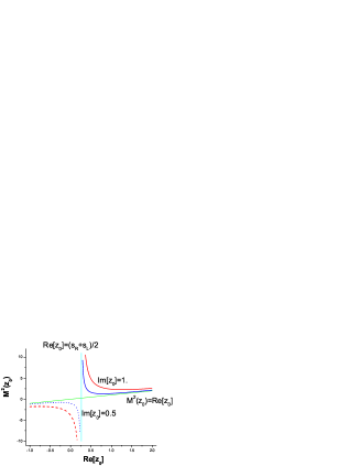
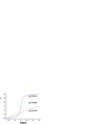
Figure 4: The left figure shows $M^{2}(z_{0})$ as a function of $\mathrm{Re}[z_{0}]$, for two choices of $\mathrm{Im}[z_{0}]$. The right figure gives some examples of resonances and their contribution to phase shift.

4.2 A Pedagogical Analysis to a Toy Model Description of Resonances

A very simple but frequently used parametrization form of $S$ matrix to fit the position of a physical resonance is the following,

$$S(s)=\frac{M^{2}-s+i\rho(s)g}{M^{2}-s-i\rho(s)g}\ .$$ (34)

where $\rho(s)$ is the kinematic factor. For equal mass like the $\pi\pi$ scatterings, $S$ matrix as described by Eq. (34) usually contains a virtual state and a pair of resonance poles on the second sheet. But Eq. (34) usually contains two pairs of resonance poles for $\pi K$ scattering due to the mass difference between $\pi$ and $K$. Fig. 5 shows the traces of two pairs of resonance poles with the increase of $g$ for different $M^{2}$. We find that $M^{2}=(s_{R}+s_{L})$ and $M^{2}=(s_{R}+s_{L})/2$ are two critical points for the two pairs of resonance poles. When $g$ increases from zero, two pairs of resonances will appear, one from the origin (due to the $1/s$ singularity hidden in the kinematic factor) and another from ($M^{2}$, 0). When $g$ increases to a certain magnitude, one pair of resonances will reach the real axis and change to two virtual states, and one of them will run upwards $s_{R}$ whereas another will run downwards $s_{L}$. If $M^{2}>(s_{R}+s_{L})$, the left pair of resonance poles generated from the origin will change into two virtual states and the right pair of resonance poles will become wider and wider but never reach the critical line $M^{2}=(s_{R}+s_{L})/2$, and if $M^{2}<(s_{R}+s_{L})$ the way of motion of the two pairs of resonance poles changes, as shown in Fig. 5.

Eq. (34) is a commonly used parametrization form of $S$ matrix to fit resonances. But from the above discussion, we know that Eq. (34) is not a parametrization of $S$ matrix for one pair of resonance poles, but usually for two pairs. Since one pair of poles is below threshold $s_{R}$ or change into two virtual states on the real axis (also below the threshold), the existence of such poles will violate the validity of chiral expansions at low energies and is therefore spurious. Actually the low lying poles in here has the same origin as the single virtual state pole in the case of equal mass scattering. [18] They are both generated from the kinematical singularity of $\rho(s)$. Whether the existence of such spurious poles strongly affects the determination of another pair of resonance poles depends on their contribution to phase shift or scattering length. For example if we set the physical resonance pole position at $\sqrt{s}=0.8\pm 0.3i$GeV then another pair of poles will locate at $\sqrt{s}=0.431\pm 0.125i$GeV. The scattering length contributed by the two are: $a=2.18$GeV^-1 for $\kappa$ and $a=4.30$GeV^-1 for the spurious pole!

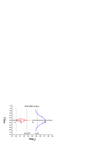
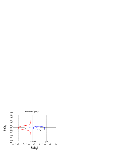
Figure 5: The traces of two pairs of resonances from Eq.(34) with the increase of $g$ for different $M^{2}$. We give two typical figures: the left figure for $M^{2}>(s_{R}+s_{L})$, and the right figure for $M^{2}<(s_{R}+s_{L})$.

At this moment the major reason to exclude Eq. (34) is rather academic. However, in sec. 5.3 we will see that the experimental data also exclude very likely the use of Eq. (34).

4.3 The Factorized $S$ Matrix and the Separable Singularities

For a general $S$ matrix, there can be many poles on the complex $s$ plane. However we can always express the complicated physical $S$ matrix into a product of many simple $S$ matrices:

$$S^{phy}=S^{cut}\cdot\prod_{i}S^{p}_{i}\ ,$$ (35)

suppose we can find all the poles of $S^{phy}$. The pole contributions, $S_{i}^{p}$, to $S^{phy}$ are parameterized using the forms given in Sec. 4.1. Now the only uncertainty remains is the cut contribution $S^{cut}$, which, by construction, contains no poles but inherits all the cut structure of the original $S^{phy}$. Hence $S^{cut}$ can be parameterized as the following:

$$S^{cut}=\exp[2i\rho(s)f(s)]\ ,$$ (36)

where $f(s)$ satisfies the following dispersion relation:

$$f(s) = f(s_{0})+{(s-s_{0})\over 2\pi i}{\int_{L}}{{\mathrm{disc_{L}}f(z)\over{(z-s)(z-s_{0})}}dz}$$ (37)

$$+ {(s-s_{0})\over\pi}{\int_{R}}{{\mathrm{Im_{R}}f(z)\over{(z-s)(z-s_{0})}}dz}\ ,$$

where $L$ denotes the left hand cut on the real axis and also the circular cut, and $R$ denotes the right hand cut starting from the second physical threshold to $\infty$. Apparently the above parametrization automatically guarantees single channel unitarity. Furthermore we get,

$$\mathrm{disc}f=\mathrm{disc}\{\frac{1}{2i\rho(s)}\log\left[S^{phy}(s)\right]\}\$$ (38)

on both $L$ and $R$. The Eq. (38) is derived, from an important property of $S^{p}_{i}$, that is $the$ $latter$ $does$ $not$ $contribute$ $to$ $any$ $discontinuity$ $of$ $f$. The reason follows: firstly we have

$$f(s) = \frac{1}{2i\rho(s)}\log\left[S^{phy}(s)/\prod_{i}S^{p}_{i}\right]$$ (39)

$$= \frac{1}{2i\rho(s)}\log S^{phy}(s)-\frac{1}{2i\rho}\sum_{i}\log S^{p}_{i}(s)\ .$$

The first equality in the above equation ensures that $f$ contains no more singularity than those cuts $S^{phy}$ contains, since poles and zeros of the two $S$ matrices on the $r.h.s.$ of the first equality exactly cancel, by definition. From the second equality, one easily understands, by comparing with the expressions of $S^{p}_{i}$ in sec. 4.1, that the $S^{p}_{i}$ contribution to $\mathrm{disc}f$ vanishes everywhere on all cuts. Therefore we have Eq. (38). Especially, when $s$ is on the real axis, Eq. (38) can be rewritten as,

$$\mathrm{Im}_{L,R}f(s)=-{1\over{2\rho(s)}}\log|S^{phy}(s)|\ ,$$ (40)

which is a consequence of real analyticity. On the right hand cut $R=[(M_{K}+M_{\eta})^{2},\infty)$, Eq. (40) can be further rewritten as an analytic expression,

$$\mathrm{Im}_{R}f(s)=-{1\over{2\rho(s)}}\log\eta(s)=-{1\over{4\rho(s)}}\log(\frac{S_{11}S_{22}}{\mathrm{det}S})\ ,$$ (41)

where the subscripts 1 and 2 mean channel $\pi K$ and channel $\eta K$, respectively (of course $S_{11}\equiv S^{phy}$, and in Eq. (41) $S$ means the $2\times 2$ $S$ matrix of couple channel scatterings). In principle, the Eq. (35) works not only in the single channel region but also works in the inelastic region. However, it should be emphasized that all poles in our formulae are on the second sheet. On the other side, the phase shift above the second physical threshold is mainly influenced by the third sheet pole rather than the second sheet pole (this is true at least for narrow resonances). Our present scheme suffers from the lacking of both theoretical and experimental knowledge on the inelasticity parameter, $\eta$. It is not difficult to imagine the worst situation one may encounter when we have only insufficient information on inelasticity: suppose in the inelastic region under concern there is no second sheet pole but only a third sheet pole. The latter however only shows its effects through Eq. (41). If we neglect the inelasticity effects due to our ignorance on $\eta$, we would have to fit the phase shift data $\delta_{2}$ using a second sheet pole. But this is certainly wrong by the assumption! Fortunately, the situation just described is not possible to happen in $\pi K$ scatterings. Because the $K\eta$ cut is very weak up to the $K\eta^{\prime}$ threshold [12], the third sheet pole and the second sheet pole should co-exist and the mass and the width of the two poles should be similar either. Therefore, for the $K^{*}(1430)$ pole we are going to introduce in the later fit we bear in mind that there are some ambiguities associate with it as discussed above but the problem should not be serious. In the later fit we will also neglect the $K\eta^{\prime}$ threshold effects which gives some further uncertainties to our final results. But the uncertainties should not be large either because we only fit the data below the $K\eta^{\prime}$ threshold where the influence from high energy cuts should be small and smooth. The uncertainties related to the right hand cut and the $K^{*}(1430)$, furthermore, should not waver our main conclusions on the $\kappa$ resonance, which is of our major concern in this paper, since the energy region where all these problems occur, is rather far from the low energy region where the $\kappa$ pole locates.

Going back to Eq. (36) again, it factorizes different singularities of the scattering $S$ matrix. Also, different contributions to the phase shift are additive:

$$\delta=\sum_{i}\delta^{p}_{i}+\delta_{BG}\ ,$$ (42)

where

$$\delta^{p}=\mathrm{Atan}\left[\frac{\rho(s)sG[z_{0}]}{M^{2}[z_{0}]-s}\right]$$ (43)

for a resonance located at $z_{0}$ (and $z_{0}^{*}$) and

$$\delta^{p}=\mathrm{Atan}\left[\frac{\rho(s)s}{s-s_{L}}\sqrt{\frac{s_{0}-s_{L}}{s_{R}-s_{0}}}\right]$$ (44)

for a virtual state located at $s_{0}$ ($s_{L}<s_{0}<s_{R}$). The bound state contribution can be obtained by simply change the sign of $r.h.s.$ of Eq. (44). For the background contribution we have

$$\delta_{BG}=\rho(s)f(s)\ .$$ (45)

Notice that the separation of pole contribution and background contribution is only a matter of convention. However, our definition of poles and background contribution has the advantage – as manifested in Eq. (40) – that it greatly simplifies the calculations on various cuts. That will be elaborated in the next section.

The approximation scheme in evaluating the cut contributions is to approximate $S^{phy}$ in Eq. (40) by $S^{\chi\mathrm{PT}}$ on $L$,

$$\mathrm{disc}f_{L}=\mathrm{disc}\{\frac{1}{2i\rho(s)}\log\left[S^{\chi\mathrm{PT}}(s)\right]\}\ .$$ (46)

Since the region where the above discontinuities are being estimated are far from the resonance region, we expect the chiral expansion (and hence our approximation scheme) works reasonably well here, at moderately low energies. Also the logarithmic form of the cut contribution automatically regulates, and hence reduces the effect of, the bad high energy behavior of the chiral amplitudes. Actually the cut integrals only need one subtraction (Various cut integrals are all subtracted at the $\pi K$ threshold throughout this paper). From these facts, we argue that our approximation scheme for evaluating cuts are reasonable, at least qualitatively. The quality of the approximation can be tested experimentally, as is done in the next section.

5 Fits to $\pi K$ Scattering Processes

Our goal is to search for resonances and to study their properties, in $\pi K$ scatterings, by analyzing the phase shift data. For this purpose, it is very important to first estimate various background contributions, which are originated from various cut integrals and the subtraction constant appeared in Eq. (37) and (42). The correct understanding to the background contributions is of course greatly helpful in the attempt to a precise determination to the pole parameters. It is even vital in answering the question whether there exists a broad resonance, like the $\kappa$ resonance under debate. Since the contribution from the background and the contribution from the broad resonance can be rather similar, the lacking of the knowledge on the former can even lead to completely misleading prediction to the latter. It is therefore necessary to study carefully the contribution of each term in Eq. (37). One of the main differences between the contribution from the background and the contribution from a broad resonance is their contribution to the scattering length. As we will show later that to evaluate the scattering length parameter $a_{0}^{1/2}$ generated from fits is very helpful in clarifying several issues, including the important question whether $\kappa$ exists or not.

5.1 The Estimation to the Background Contributions

Our method of estimating the ‘left hand cut’ contribution is to substitute $S^{phy}$ in Eq. (40) by $S^{\chi PT}$. The background contribution from the left hand cut is then evaluated by calculating the left hand cut integral in Eq. (37). The once subtracted integral is convergent and the integration is formally performed from $-\infty$ to $s_{L}$ on the real $s$ axis. However, since there is no reliable method to estimate correctly the contribution from large negative $s$ region, it is more appropriate to truncate the integration along the negative real $s$ axis at $\Lambda^{2}_{L}$. This introduces an additional cutoff parameter and we will test the dependence of the fit results on this parameter.

The discussions made above clearly shows how approximations enter into our scheme. It is necessary to first justify our approximation scheme. Fortunately it is possible to test whether it is reasonable to use $\chi$PT to calculate the background contributions. Because in the I=3/2 channel there are only background contributions. So we can compare directly the background contributions from our approximation with experiments. We have already demonstrated in sec. 3 that the Padé approximation gives poor description in this channel to the background contribution. Here we compare $\mathrm{Im}_{L}f(s)$ both using $S^{\chi\mathrm{PT}}$ and the [1,1] Padé $S$ matrix, as shown in figs. 6 and 7. We find once again that the Padé approximation result is poorer in reproducing the phase shift data comparing with the $\chi$PT result after adjusting the cutoff parameter within reasonable ranges. Notice that throughout this paper we do not attempt to make the global fit by varying those $L_{r}^{i}$ parameters since the $L_{r}^{i}$ parameters are in principle threshold parameters. However, several different results on the low energy constants found in the literature are tested and it is found that the influences from the different choices to the final fit results are very small. From fig. 7 disagreement between the theoretical calculation based on $\chi$PT and the experimental data is found. Better agreement can be achieved only by allowing $a_{0}^{3/2}$ to be much larger than its $\chi$PT value. Nevertheless it is verified that the problem in the I=3/2 channel has rather small influence to the $\kappa$ pole problem. Further discussions on this point will be given later.

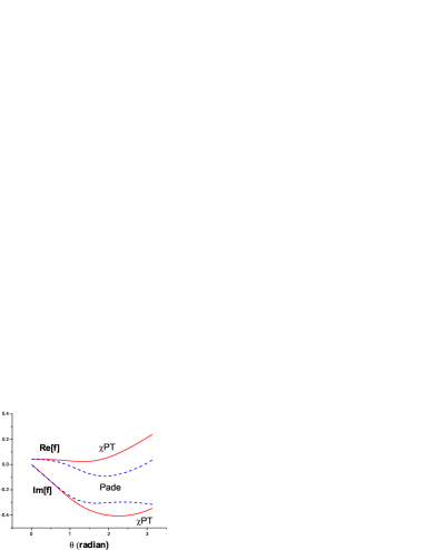
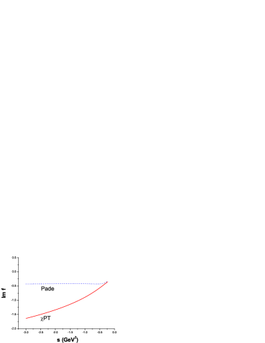
Figure 6: Various results on $\mathrm{Im}_{L}f(s)$ or $f$ from $\chi$PT and Padé approximation in I=3/2 $s$ wave $\pi K$ scattering. Left: outside the circular cut; right: on $L=(-\infty,-(M_{K}^{2}-M_{\pi}^{2})]$. The $L^{i}_{r}$ constants are taken from Eq. (3).

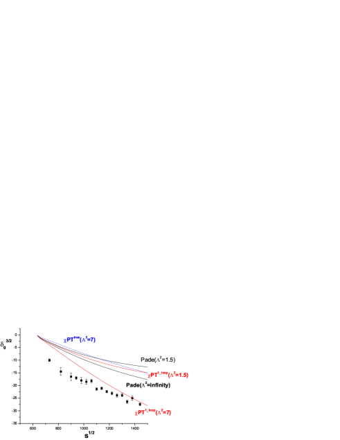
Figure 7: Theoretical results on $\delta_{0}^{3/2}$ versus the data [5]. The dashed line corresponds to the tree level $\chi$PT result. Other lines are distinguished from the labels in the figure. See footnote 6 for more explanations.

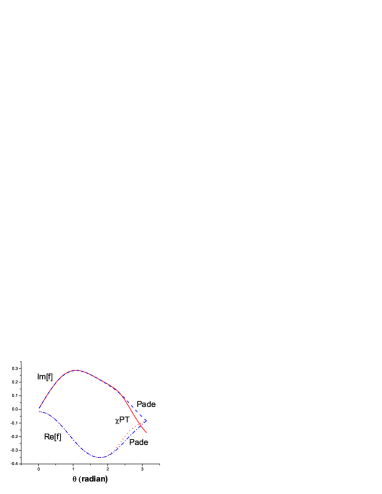
Figure 8: Various results of $f$ and $\mathrm{Im}_{L}f(s)$ from $\chi$PT and Padé approximation in the I=1/2 channel. Left: outside the circular cut; right: on $L=(-\infty,-(M_{K}^{2}-M_{\pi}^{2})]$.

In the I=1/2 channel a direct check on the background contribution is impossible since this is the channel where we will test the existence of the $\kappa$ resonance. However from the experience in the I=3/2 channel we expect that the $\chi$PT results on $\mathrm{Im}_{L}f(s)$ works also well, at least qualitatively. It is worth pointing out that the results from the [1,1] Padé approximant are rather similar to the $\chi$PT results in the I=1/2 channel, except at large negative s region. Therefore we will use the $\chi$PT prediction on $\mathrm{Im}_{L}f(s)$. In the I=1/ 2 channel, there exists also the right hand cut from $s=(M_{K}+M_{\eta})^{2}$ but it is very weak till another threshold $s=(M_{K}+M_{\eta^{\prime}})^{2}$ is reached. For the right hand cut, $\chi$PT result is totally misleading because it violates single channel unitarity in the physical region. On the other side, the Padé result maintains single channel unitarity but may give a too large contribution to the inelasticity parameter, starting from $(M_{K}+M_{\eta})^{2}$. Since experiments suggest that the inelasticity is very small till $(M_{K}+M_{\eta^{\prime}})^{2}$ and the latter is already very far from the low energy region we are interested in, we during the fit simply set the right hand cut contribution being vanish. As is already discussed in sec. 4.3, this approximation may have some effects to the determination of the $K(1430)$ resonance but should have negligible influence to the $\kappa$ resonance.

5.2 The Numerical Analysis and Data Handling

The two experiments on $K\pi$ scatterings we will make use of are from the LASS Collaboration [4] and Estabrooks et al. [5]. The latter gives the phase shift data in the I=1/2 channel for $\sqrt{s}=0.73-1.3$GeV and in the I=3/2 channel for $\sqrt{s}=0.73-1.72$GeV. It is found that the scattering is purely elastic up to 1.3GeV, i.e., $\eta_{0}^{1/2}=\eta_{0}^{3/2}=1$ in this region. In the I=3/2 channel the inelasticity can be neglected in the whole energy range. The experiment by the LASS Collaboration only measures the $K^{-}\pi^{+}$ channel and hence only affords the following combination of data:

$$A_{0}=a_{0}e^{i\phi_{0}}=T_{0}^{1/2}+\frac{1}{2}T_{0}^{3/2}=\frac{1}{2i}(\eta_{0}^{1/2}e^{2i\delta^{1/2}_{0}}-1)+\frac{1}{4i}(\eta_{0}^{3/2}e^{2i\delta^{3/2}_{0}}-1)\ ,$$ (47)

for $\sqrt{s}=0.825-2.52$GeV. Notice that in the above equation the definition of $T$ matrix is different from previously used in this paper.

In this work our discussion will be confined to the single channel approximation, though it is understood that our formalism in principle works also in the inelastic region. The validity domain of single channel approximation is largely expanded in $\pi K$ scatterings since the second threshold, the $K\eta$ channel opens very weakly in agreement with $SU(3)_{f}$ expectations, and so any inelasticity can be neglected until one reaches the $K\eta^{\prime}$ threshold [12]. Therefore we in the fit assume elasticity up to the $K\eta^{\prime}$ threshold both in I=1/2 and 3/2 channels. As illustrated in the Introduction the main purpose of this paper is to study whether there exists the $\kappa$ resonance and, if exists, its properties. The approximation of neglecting the inelasticity effects will mainly affect the well established $K^{*}(1430)$ resonance which is not our main interest here.

Our strategy of making the fit follows: assuming two resonances, one for $K^{*}(1430)$, another one for the $\kappa$ resonance under investigation and the two complex poles contribute four parameters. There are another two parameters coming from the two scattering lengths, i.e., $a_{0}^{1/2}$ and $a_{0}^{3/2}$ (or equivalently, two subtraction constants). Therefore there are totally 6 parameters in the fit. The first fit only make use of the LASS data up to $\sqrt{s}=1.43$GeV, which is about 20MeV below the $K\eta^{\prime}$ threshold and consist of 60 data points. We call it Method I hereafter. In the second fit we also include data from Estabrooks et al., up to $\sqrt{s}=1.3$GeV in the I=1/2 channel and up to $\sqrt{s}=1.43$ in the I=3/2 channel. This will add another 41 data points, among them 24 come from the $\delta_{0}^{1/2}$ phase shift data and 17 from the $\delta_{0}^{3/2}$ phase shift data. We call this fit scheme Method II hereafter. Treatment to various cuts are already illustrated in sec. 5.1.

5.3 The fit to the LASS data (Method I)

This part of discussion is divided into two subsections: one is the fit without considering further constraints from chiral perturbation theory except when estimating the left hand cut contributions. The second subsection respects the $\chi$PT results, especially its predictions on the scattering length parameters. Since what is involved here is the SU(3) version of $\chi$PT and since there exists possible conflict between theory and experiments, we think it is worthwhile to be cautious to make the separate discussions.

5.3.1 The fit without constraints from $\chi$PT

Using MINUIT, we perform the six parameters fit ($a_{0}^{1/2}$, $a_{0}^{3/2}$ and four pole parameters for $\kappa$ and $K^{*}(1430)$) to the LASS data up to 1430MeV. Except for these 6 fit parameters we have, as already stressed, one additional but somewhat unpleasant parameter: the cutoff parameters responsible for the truncation of left hand integrals in both I=1/2 and 3/2 channels, denoted as $\Lambda_{L}^{2}$. The fit results will of course depend on the cutoff parameter, nevertheless the dependence is much weaker than that of Ref. [16] which is of course progressive. In table 2 we list various results obtained by varying $\Lambda^{2}_{L}$ from which we draw the following conclusions:

1. The overall $\chi^{2}$ is rather stable against most changes of the cutoff parameters, and the fit prefers $\Lambda^{2}_{L}\simeq 1.5$GeV². This is supported by an independent analysis to the phase shift data provided by Ref. [5]. It should be emphasized that these conclusions are obtained only when $a_{0}^{1/2}$ and especially $a_{0}^{3/2}$ are treated as completely free in the fit. If $a_{0}^{3/2}$ is confined to its $\chi$PT value, the best $\Lambda^{2}_{L}$ value will be enhanced.

2. The fit result on $a_{0}^{3/2}$ is rather sensitive to the cutoff parameter. Actually these sensitivity are only related to the cutoff parameter in the I=3/2 channel rather than that in the I=1/2 channel (see also footnote 7 and fig. 7). Remember that we are fitting the combined data now, therefore our method can somehow rather clearly distinguish different channel contributions to the LASS data.

3. Except for the problem mentioned above, most other results are rather stable against the variation of $\Lambda_{L}^{2}$ in a reasonable range. This is even true when we confine $a_{0}^{1/2}$ and $a_{0}^{3/2}$ in the fit. See later text for more discussions.

To save the already lengthy discussions we in the following will only exhibit results for the fixed value of the cutoff parameters: $\Lambda^{2}_{L}=1.5$GeV², unless otherwise stated. However we also carefully analyzed the uncertainties of all our major outputs induced by the uncertainties of the cutoff parameters and found out that the uncertainties are not magnificent.

$\Lambda^{2}_{L}$	$\chi^{2}_{tot}$	$a_{0}^{1/2}$	$a_{0}^{3/2}$	$M_{\kappa}$	$\Gamma_{\kappa}$
1	38.64	$0.292\pm 0.100$	$-0.143\pm 0.006$	$573\pm 108$	$747\pm 438$
1.5	38.35	$0.284\pm 0.089$	$-0.129\pm 0.006$	$594\pm 79$	$724\pm 332$
2	39.44	$0.278\pm 0.078$	$-0.118\pm 0.006$	$609\pm 58$	$711\pm 272$
2.5	41.30	$0.274\pm 0.087$	$-0.109\pm 0.006$	$620\pm 61$	$703\pm 258$
3	43.55	$0.271\pm 0.129$	$-0.102\pm 0.006$	$629\pm 81$	$697\pm 354$
3.5	45.96	$0.268\pm 0.077$	$-0.096\pm 0.006$	$636\pm 40$	$693\pm 236$
5	53.18	$0.262\pm 0.068$	$-0.082\pm 0.006$	$652\pm 30$	$685\pm 191$
10	71.40	$0.254\pm 0.062$	$-0.060\pm 0.006$	$676\pm 24$	$673\pm 148$
$\infty$	120	$0.242\pm 0.067$	$-0.026\pm 0.007$	$716\pm 16$	$653\pm 136$

Table 2: Various fit results to the LASS data up to 1.43GeV obtained by varying the cutoff parameters of the left hand integrals. There are totally 60 data points and 6 parameters. Various results on $K^{*}(1430)$ are similar and are not listed here. All values of mass parameters in the table are in units of MeV.

As is shown in table 2, the global fit prefers larger magnitudes of the scattering lengths than those predicted by $O(p^{4})$ $\chi$PT [13], which are: $a_{0}^{1/2}=0.18\pm 0.02$, $a_{0}^{3/2}=-0.05\pm 0.02$. The present fit gives however rather large error bars on $a_{0}^{1/2}$. To further test the dependence of the $\kappa$ pole on $a_{0}^{1/2}$ we also perform the fits by varying $a_{0}^{1/2}$ while keeping it fixed during each fit. The results are shown in fig. 9. In fig. 9 we have not shown the situation when $a_{0}^{1/2}>0.4$ where the results become more and more unstable. From fig. 9 we may have the impression that when $a_{0}^{1/2}$ is roughly less than 0.35 the $\kappa$ resonance seems to exist. If $a_{0}^{1/2}$ is greater than the value the existence of the resonance becomes doubtful. This observation will be further examined in the following discussions.

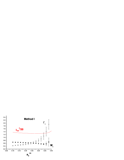
Figure 9: The dependence of the mass, width and their error bars of the $\kappa$ resonance on $a_{0}^{1/2}$ (Method I). The fits contain only 5 parameters. Taking $\Lambda_{L}^{2}=1.5$GeV².

The full results of the six parameters fit to the LASS data are the following:

$$\chi^{2}_{d.o.f.}=38.35/(60-6)\ ;$$ (48)

$$M_{\kappa}=594\pm 79MeV\ ,\,\,\,\Gamma_{\kappa}=724\pm 332MeV\ ;$$

$$a_{0}^{1/2}=0.284\pm 0.089\ ,\,\,\,a_{0}^{3/2}=-0.129\pm 0.006\ ;$$

$$M_{K^{*}}=1456\pm 8MeV\ ,\,\,\,\Gamma_{K^{*}}=217\pm 31MeV\ .$$

The corresponding fit results are plotted in fig. 10.

  

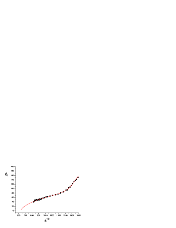
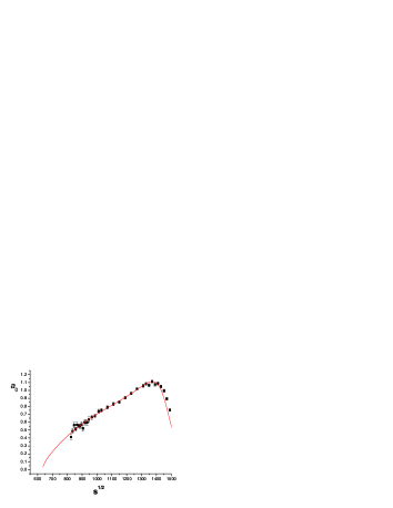
Figure 10: Fit results (Eq. (48)) to $\phi_{0}$ (left) and $a_{0}$ (right) using Method I. The data are fitted only up to 1430MeV but are shown up to 1500MeV.

Since their is no separate data of I=1/2 and I=3/2 channels provided by the LASS Collaboration, we also plot curves of $\delta_{0}^{1/2}$ and $\delta_{0}^{3/2}$ from our fit results versus the phase shift data from Estabrooks et al. in fig. 11. We stress again that in the present fit the LASS data are combined data from both the I=1/2 and I=3/2 channels. From fig. 11 we find that the present method can rather clearly distinguish different contributions from different channels.

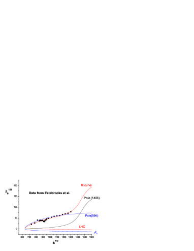
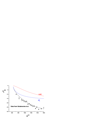
Figure 11: The comparison between the fit results on the LASS data (Eq. (48)) and the data from Estabrooks et al. [5].

In order to answer the question whether $\kappa$ exists or not, we further freeze the $\kappa$ degrees of freedom in the fit and we get

$$\chi^{2}_{d.o.f.}=63.67/(60-4)\ ;$$ (49)

$$M_{\kappa}=--\ ,\,\,\,\Gamma_{\kappa}=--\ ;$$

$$a_{0}^{1/2}=0.446\pm 0.006\ ,\,\,\,a_{0}^{3/2}=-0.130\pm 0.006\ ;$$

$$M_{K^{*}}=1432\pm 3MeV\ ,\,\,\,\Gamma_{K^{*}}=314\pm 20MeV\ .$$

Comparing with the results in Eq. (48) the $\chi^{2}_{d.o.f.}$ given by Eq. (49) is increased by a factor of 1.7. If this is not enough to support the existence of $\kappa$, the value of $a_{0}^{1/2}$ given by Eq. (49) is too large comparing with the $\chi$PT value. While the fit value of $a_{0}^{3/2}$ is about 4 $\sigma$ away from $\chi$PT result, $a_{0}^{1/2}$ as predicted by Eq. (49) is 14$\sigma$ away! It is actually easy to understand why the fit program is forced to chose such a large $a_{0}^{1/2}$. Looking at fig. 11, when the contribution of the $\kappa$ resonance is withdrawn the subtraction constant has to be much increased to fit data. Since the $\rho f_{0}$ contribution increase faster at threshold than the $\kappa$ contribution and slower at higher energies than the $\kappa$ contribution, this leads to a larger $a_{0}^{1/2}$.

It is also worthwhile to investigate the fit using Eq. (34) to parameterize $\kappa$. The result follows:

$$\chi^{2}_{d.o.f.}=38.22/(60-6)\ ;$$

$$M_{\kappa}=726\pm 8MeV\ ,\,\,\,\Gamma_{\kappa}=698\pm 19MeV\ ;$$

$$a_{0}^{1/2}=0.403\pm 0.025\ ,\,\,\,a_{0}^{3/2}=-0.129\pm 0.006\ ;$$

$$M_{K^{*}}=1453\pm 3MeV\ ,\,\,\,\Gamma_{K^{*}}=220\pm 18MeV\ ,$$ (50)

and the spurious resonance pole locates at (the central value): $M=477$MeV, $\Gamma=94$MeV. Comparing with Eq. (48), the total $\chi^{2}$ given by Eq. (5.3.1) is very similar, but it gives a too large $a_{0}^{1/2}$ comparing with the $\chi$PT prediction. Therefore Eq. (34) is very likely to be excluded by the LASS data.

5.3.2 The fit with constraints from $\chi$PT

It is sometimes found in the literature the discussions on the constraint of the Adler zero on the scattering amplitude. [25] In our scheme, it is possible to embed this constraint into our parametrization form, similar to what is done in Ref. [17]. However, the Adler zero automatically emerges in our approach if the subtraction constant $f_{0}$ is limited within certain range. This is because all the resonance(and virtual state) $S$ matrices are real and less than 1 when $s_{L}<s<s_{R}$. On the contrary the cut integrals contribute a factor larger than 1, therefore a $T$ matrix zero emerges in the right place when $f_{0}$ is confined to a certain range, which in turn put some constraints on the magnitude of the scattering length parameter itself. For example, within the range $0<a_{0}^{1/2}<0.26$ (see fig. 9) there exists a $T$ matrix zero in the region $s_{L}<s<s_{R}$, and when $a_{0}^{1/2}\simeq 0.20$ the zero locates in the place close to the one loop $\chi$PT prediction. We make further fit by confining $a_{0}^{1/2}$ in the region $0.18\pm 0.02$ and the results follow:

$$\chi^{2}_{d.o.f.}=38.96/(60-6)\ ;$$ (51)

$$M_{\kappa}=646\pm 7MeV\ ,\,\,\,\Gamma_{\kappa}=540\pm 42MeV\ ;$$

$$a_{0}^{1/2}=0.2\ ,\,\,\,a_{0}^{3/2}=-0.128\pm 0.006\ ;$$

$$M_{K^{*}}=1450\pm 5MeV\ ,\,\,\,\Gamma_{K^{*}}=232\pm 25MeV\ .$$

The Adler zero position is now at $s_{A}\simeq 0.245$GeV to be compared with the 1–loop $\chi$PT value $s_{A}\simeq 0.233$GeV. The necessity for the existence of the $\kappa$ resonance may be best illustrated by the fit when constraining $a_{0}^{1/2}$ to lie within the range as predicted by $\chi$PT value, $a_{0}^{1/2}=0.18\pm 0.02$ and meanwhile freeze out $\kappa$. Under this situation $a_{0}^{0}$ will reach its upper value at 0.2 and the $\chi^{2}_{tot}\sim 750$! Comparing with the value of $\chi^{2}_{tot}$ in Eqs. (51) and (48), it clear demonstrates the necessity to include the $\kappa$ resonance if $a_{0}^{1/2}$ is close to (or not much larger than) its $\chi$PT value.

The next question is to ask what would happen if we further confine both $a_{0}^{1/2}$ and $a_{0}^{3/2}$ to their $\chi$PT value? The answer is,

$$\chi^{2}_{d.o.f.}=127.6/(60-6)\ ;$$

$$M_{\kappa}=655\pm 9MeV\ ,\,\,\,\Gamma_{\kappa}=549\pm 42MeV\ ;$$

$$a_{0}^{1/2}=0.2\ ,\,\,\,a_{0}^{3/2}=-0.07\ ;$$

$$M_{K^{*}}=1465\pm 5MeV\ ,\,\,\,\Gamma_{K^{*}}=258\pm 33MeV\ .$$ (52)

Though the $\chi^{2}_{tot}$ is now much enhanced as comparing with the result given by Eq. (51), we are very much consoled by the nice agreement on the $\kappa$ pole between the two methods. This again suggests that though we fit the LASS data which is a combined effect of both the I=1/2 channel and the I=3/2 channel, the present approach can somehow clearly distinguish different contributions from different channels. Actually if we make a plot like fig. 11 we find that the fit curve in the I=1/2 channel still agrees well with the data whereas in the I=3/2 channel there exists rather large deviations. Technically, the large $\chi^{2}_{tot}$ appeared in Eq. (5.3.2) can be reduced roughly by half when increasing $\Lambda_{L}^{2}$ (or more precisely, increasing the cutoff parameter in the I=3/2 channel). This ambiguity with respect to the cutoff parameter will contribute, though not large, some uncertainties to the pole positions, which can be considered as the ‘systematic’ error in our approach.

5.4 The combined data fit (Method II)

The data from Estabrooks et al. contain some problems. This can be clearly seen from fig. 11. The dip structure of the phase shift data around 920MeV apparently leads to $\frac{d\delta}{ds}<0$. According to our analysis, it cannot be explained by the smooth background contributions. If the dip structure were true it unavoidably leads to very complicated pole structures and causality violation conclusion. The dip structure actually gives a large contribution to the total $\chi^{2}$ in the combined fit to both the LASS data and the data from Estabrooks et al.. Nevertheless we still make the combined fit using the method as described previously. The result for six free parameters fit follows:

$$\chi^{2}=266.9/(101-6)\ ;$$

$$M_{\kappa}=898\pm 315MeV\ ,\,\,\,\Gamma_{\kappa}=1902\pm 282MeV\ ;$$

$$a_{0}^{1/2}=0.384\pm 0.017\ ,\,\,\,a_{0}^{3/2}=-0.136\pm 0.002\ ;$$

$$M_{K^{*}}=1468\pm 4MeV\ ,\,\,\,\Gamma_{K^{*}}=146\pm 23MeV\ .$$ (53)

We see from the above equation that the $\chi_{d.o.f.}^{2}$ is much larger than the fit using only the LASS data and the scattering length parameter is much larger than the $\chi$PT value and the result should not be trustworthy. We also plot the fit results versus the $\delta_{0}^{1/2}$ data in fig. 12.

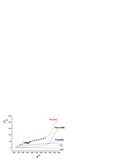
Figure 12: The combined fit results (Eq. (5.4)) on $\delta_{0}^{1/2}$.

It is interesting to notice that the results of $M_{\kappa}$ and $\Gamma_{\kappa}$ and their error bars obtained by varying $a_{0}^{1/2}$, as shown in fig. 13, have a very similar behavior to the results obtained using Method I as shown in fig. 9, for small value of $a_{0}^{1/2}$. Therefore, though not successful, the combined fit still confirms the conclusion that the $\kappa$ resonance exists if $a_{0}^{1/2}$ does not deviate too much from its $\chi$PT value.

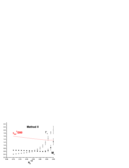
Figure 13: The dependence of the mass, width and their error bars of the $\kappa$ resonance on $a_{0}^{1/2}$ (Method II). Taking $\Lambda_{L}^{2}=1.5$GeV².

6 Summary and Conclusions

We have already made a rather long and detailed discussion on the new unitarization approach and the results on the $\kappa$ pole based on the approach. In here we summarize our main physical results: first of all, there exists the $\kappa$ resonance, if the scattering length parameter $a_{0}^{1/2}$ does not deviate much from its $\chi$PT prediction. Secondly, according to our fit to the LASS data, the mass of the $\kappa$ resonance is definitely smaller than most previous results found in the literature. It is found that the width parameter is more flexible than the mass parameter in the fit results, which can also be seen in fig. 9. Our fit results are given in Eq. (48). If we further fix $a_{0}^{1/2}$ to be its current $\chi$PT value within 1$\sigma$ error bar, the pole position of $\kappa$ is approximately given by Eq. (51). However, unlike $\pi\pi$ scatterings, the scattering lengths under concern are from SU(3) $\chi$PT results and one expects that high order corrections are more significant here. Therefore one should also be cautious when referring to Eq. (51) or (5.3.2). Furthermore, there are some mismatch or disagreement between our method and numerical results and the experimental data which predominately come from the I=3/2 channel. However, we have made efforts to separate and to minimize the ambiguity when fixing the location of the $\kappa$ pole. In fact, we are convinced by comparing Eqs. (51) and (5.3.2) that the problem in the I=3/2 channel has only minor influence to the $\kappa$ pole location.

Our numerical results, especially Eq. (5.3.2) and the way they are derived are in principle consistent with that of Ref. [12] in which $\kappa$ pole with similar location can be found after adding a few ‘data points’ generated by $\chi$PT to the original LASS data. These ‘data points’ should take the similar role as constraining the scattering lengths here. The present approach also share some similarities, at qualitative level, with that of Ref. [7], though in details the two approaches differ in the treatment on both the pole contributions and the cut contributions.

While this paper is being completed, we received a paper by Büttiker, Descotes and Moussallam [27]. The central value of $a_{0}^{1/2}$ given in Ref. [27] obtained by solving Roy–Steiner equation increases considerably than that of Ref. [13], and $a_{0}^{3/2}$ changes very little. Apparent disagreement on $\delta^{3/2}_{0}$ between the result of Ref. [27] and the experimental data are also indicated. If we take roughly $a_{0}^{1/2}\sim 0.201-0.245$ as indicated by the results of Ref. [27] (also $a_{0}^{3/2}$ is readjusted to lie within the range -0.053 – -0.038), we would obtain, similar to obtaining Eq. (5.3.2), table 3.

$\Lambda^{2}_{L}$	$\chi^{2}_{tot}$	$a_{0}^{1/2}$	$a_{0}^{3/2}$	$M_{\kappa}$	$\Gamma_{\kappa}$
1.5	186.1	$0.201\pm 0.038$	$-0.053(\rm{at\,\,limit})$	$666\pm 11$	$565\pm 41$
3	104.7	$0.201\pm 0.043$	$-0.053(\rm{at\,\,limit})$	$673\pm 10$	$562\pm 35$
5	75.2	$0.201\pm 0.026$	$-0.053(\rm{at\,\,limit})$	$681\pm 11$	$567\pm 34$
7	69.8	$0.218\pm 0.026$	$-0.053(\rm{at\,\,limit})$	$682\pm 25$	$598\pm 153$
9	71.1	$0.234\pm 0.032$	$-0.053(\rm{at\,\,limit})$	$682\pm 24$	$629\pm 134$
11	74.6	$0.243\pm 0.032$	$-0.053\pm 0.009$	$683\pm 16$	$651\pm 85$
20	90.1	$0.245\pm 0.021$	$-0.044\pm 0.006$	$693\pm 14$	$658\pm 40$
$\infty$	137.4	$0.245(\rm{at\,\,limit})$	$-0.038(\rm{at\,\,limit})$	$710\pm 14$	$661\pm 29$

Table 3: Various fit results to the LASS data up to 1.43GeV obtained by varying the cutoff parameters of the left hand integrals and with the constraints on $a_{0}^{1/2}$ and $a_{0}^{3/2}$ from Ref. [27]. All values of $M_{\kappa}$ and $\Gamma_{\kappa}$ in the table are in units of MeV.

Again, when there is a large $\chi^{2}$ occurs in table 3 it is mainly contributed by the I=3/2 channel. The ‘systematic’ errors induced by varying cutoff parameters are estimated and the final results on the $\kappa$ pole position obtained by considering the constraints provided by Ref. [27] is estimated from table 3:

$$M_{\kappa}=688\pm 25\pm 22{\mathrm{M}eV}\ ,\,\,\,\Gamma_{\kappa}=613\pm 153\pm 48{\mathrm{M}eV}\ .$$ (54)

Here the first error bar corresponds to the largest error bar generated by MINUIT when varying the cutoff parameters. The second error bar is our estimate obtained by examining the variation of the corresponding central value when changing the cutoff parameters, which is also a rather conservative estimate.

Acknowledgement We would like to thank Prof. Y. S. Zhu for helpful discussions on data fittings. This work is supported in part by China National Natural Science Foundation under grant number 10047003 and 10055003.

References

- [1] R. Jaffe, Phys. Rev. D15(1977)267; Phys. Rev. D15(1977)281.
- [2] E. M. Aitala (E791 Collaboration), Phys. Rev. Lett.89(2002)121801.
- [3] J. Z. Bai (BES Collaboration), hep-ex/0304001.
- [4] D. Aston (LASS Collaboration), Nucl. Phys. B296(1988)493.
- [5] P. Estabrooks , Nucl. Phys. B133(1978)490.
- [6] E. Van Beveren , Z. Phys. C30(1986)615.
- [7] S. Ishida , Prog. Theor. Phys. 98(1997)621.
- [8] D. Black , Phys. Rev. D58(1998)054012.
- [9] M. Jamin, J. A. Oller and A. Pich, Nucl. Phys. B587(2000)331.
- [10] N. A. Tornqvist, Z. Phys. C68(1995)647.
- [11] A. V. Anisovich and A. V. Sarantsev, Phys. Lett. B413(1997)137.
- [12] S. N. Cherry and M. R. Pennington, Nucl. Phys. A688(2001)823.
- [13] Ulf-G.Meissner, Nucl. Phys. B357(1991)129.
- [14] V. Bernard, N. Kaiser, Ulf-G. Meissner, Phys. Rev. D 1990.
- [15] H. Q. Zheng, Z. Y. Zhou, G. Y. Qin and Z. G. Xiao, talk given at Tenth International Conference On Hadron Spectroscopy, August 31 - September 6, 2003, Aschaffenburg, Germany (hep-ph/0309242).
- [16] Z. G. Xiao and H. Q. Zheng, Nucl. Phys. A695 (2001)273.
- [17] J. Y. He, Z. G. Xiao and H. Q. Zheng, Phys. Lett. B526(2002)59; Erratum: . B549(2002)362.
- [18] H. Q. Zheng, Talk given at International Symposium on Hadron Spectroscopy, Chiral Symmetry and Relativistic Description of Bound Systems, Tokyo, Japan, 24-26 Feb 2003, hep-ph/0304173.
- [19] See for example, A. Dobado and J. R. Peláez, Phys. Rev. D56(1997)3057; J.A.Oller, E.Oset and A.Ramos, Prog.Part.Nucl.Phys. 45(2000)157.
- [20] G. Y. Qin , Phys. Lett. B542(2002)89.
- [21] J. Kennedy and T. D. Spearman, Phy. Rev. 126 (1962)1596.
- [22] J. Gasser and H. Leutwyler, Nucl. Phys. B250(1985)465.
- [23] Z. G. Xiao and H. Q. Zheng, Chin. Phys. Lett. 20(2003)342.
- [24] Z. G. Xiao and H. Q. Zheng, Preprint hep-ph/0103042.
- [25] See for example, D. Bugg, Phys. Lett. B572(2003)1 and references therein.
- [26] H. Q. Zheng , in progress.
- [27] P. Büttiker, S. Descotes-Genon and B. Moussallam, talk given at QCD’03 conference, 2-9 July 2003, Montpellier; hep-ph/0310045.