Abstract

In the minimal supersymmetric standard model, tau sleptons $\tilde{\tau}_{1,2}$ and neutralinos $\tilde{\chi}^{0}_{1,2}$ are expected to be among the lightest supersymmetric particles that can be produced copiously at future $e^{+}e^{-}$ linear colliders. We analyze $\tilde{\tau}$ pair and $\tilde{\chi}_{1}^{0}\tilde{\chi}_{2}^{0}$ production under the assumption $m_{\tilde{\chi}_{1}^{0}}<m_{\tilde{\tau}_{1}}<m_{\tilde{\chi}_{2}^{0}}$, allowing the relevant parameters of the SUSY Lagrangian to have complex phases. We show that the transverse and normal components of the polarization vector of the $\tau$ lepton produced in $\tilde{\chi}_{2}^{0}$ decays offer sensitive probes of these phases.

1 Introduction

In extending the standard model (SM) of strong and electroweak interactions, supersymmetry (SUSY) provides a well–motivated framework with several virtues [1]. Weak–scale SUSY has its natural answer to the gauge hierarchy problem [2], achieves gauge unification without the ad hoc introduction of additional particles [3], and radiatively explains the electroweak symmetry breaking in terms of the large top quark mass [4]. Moreover, $R$ parity conserving SUSY offers a compelling candidate for the cold dark-matter component of the Universe [5].

Since none of the superpartners has been found, SUSY is apparently broken if it exists at all. Only soft breaking terms are allowed, however, if SUSY is meant to solve the hierarchy problem. Even though this softness leads to experimentally accessible signatures of the superpartners, the presence of many new (generally complex) parameters complicates the phenomenological situation: Without a specific mechanism for SUSY breaking, even in the minimal supersymmetric standard model (MSSM) more than one hundred new parameters are introduced [6]. Therefore precision measurements of these soft breaking terms as well as other fundamental SUSY parameters are essential to explore the SUSY breaking mechanism. Here we discuss how to extract the parameters, in particular the CP–odd phases, in the scalar tau (stau) and neutralino sectors of the MSSM. Recall that CP–odd phases are needed [7] for the dynamical generation of the baryon asymmetry of the Universe; the phase in the CKM (quark mixing) matrix is most likely not sufficient.

The third generation scalars’ CP phases have drawn a lot of interest as these phases can be large without any conflict with experimental constraints. In contrast, the first two generation sfermions are severely constrained by measurements of the electric dipole moments of the electron, muon, and neutron [8]: Either their CP violating phases are very small or their masses are very large, well above 1 TeV, or parameters are adjusted such that different contributions cancel to very good precision [9]. Apart from the absence of a well-established mechanism to suppress the CP violating phases for the first two generations, other difficulties such as potentially large flavor changing neutral currents [10], and rapid proton decay through dimension five operators in SUSY GUTs [11], prefer very heavy first two generation sfermions [12]. In contrast, third generation sfermions are expected to be light (“inverted hierarchy”) due to their central role in the naturalness problem as well as due to their large Yukawa couplings which substantially reduce their masses at the electroweak scale. Therefore, ${\cal O}(1)$ CP violating phases and relatively small masses of third generation sfermions are well motivated and phenomenologically viable.

The stau sector may well allow the first measurement of CP violating phases of sfermions at a future linear collider (FLC) with c.m. energy of up to 500 GeV: In inverted hierarchy models, only some light neutralinos, charginos and third–generation sfermions are expected to be produced at the FLC whereas the other supersymmetric particles are not accessible [13]. Our main focus is on the CP violating phase in the stau sector, $\phi_{\tilde{\tau}}$. This phase is associated with $\tilde{\tau}_{L}-\tilde{\tau}_{R}$ mixing, which in turn is enhanced for large values of the ratio $\tan\beta$ of Higgs vacuum expectation values. Note that $\tan\beta$ as high as $50$ is preferred in some $SO(10)$ grand unified models with Yukawa unification [14]. In contrast, scenarios with $\tan\beta$ near unity are severely constrained by Higgs searches at LEP [15]. We will see that $\tan\beta=10$ is sufficient to generate large CP–violating effects.

A phenomenologically significant question is which observable is sensitive to the phase $\phi_{\tilde{\tau}}$. The stau is expected to be advantageous in constructing CP-odd observables since one of its decay products, the tau lepton, also decays, which enables us to measure the tau polarization. In the simplest decay channel ${\tilde{\tau}}^{\pm}\to\tau^{\pm}{\tilde{\chi}^{0}}_{1}$, however, the invisibility of the LSP ${\tilde{\chi}^{0}}_{1}$ allows only two measurable vectors, the three-momentum and polarization vector of the tau: No CP–odd observable can be constructed. Among two-step cascade decays, the decay of the second lightest neutralino ${\tilde{\chi}^{0}}_{2}$ into a stau and a tau lepton, followed by the stau decay, is one of the most promising candidates especially if $\tan\beta$ is not small. $\tilde{\chi}_{1}^{0}\tilde{\chi}_{2}^{0}$ production has one of the lowest threshold energies of all SUSY processes that lead to visible final states. Moreover, if $m_{\tilde{\chi}_{1}^{0}}<m_{\tilde{\tau}_{1}}<m_{\tilde{\chi}_{2}^{0}}$, the decay $\tilde{\chi}_{2}^{0}\rightarrow\tilde{\tau}_{1}^{\pm}\tau^{\mp}$ has a large branching ratio, often near 100%. Finally, CP–odd observables can be constructed, since the $\tilde{\chi}_{2}^{0}$ in the intermediate state is polarized. Previous studies [16] have focused on $\chi_{2}^{0}\rightarrow\ell^{+}\ell^{-}\tilde{\chi}_{1}^{0}$ decays $(\ell=e,\,\mu,\,\tau)$, using the triple product of the $\ell^{\pm}$ 3–momenta with the incident $e^{-}$ beam 3–momentum as CP–odd observable. This allows to probe CP violation in the neutralino sector, but is not sensitive to $\phi_{\tilde{\tau}}$. Here we focus on the case $\ell=\tau$, and construct CP–odd observables involving the spin of of the $\tau$ lepton produced in the first step of $\tilde{\chi}_{2}^{0}$ decay.

Our purpose in this paper is to show that these observables are indeed sensitive to $\phi_{\tilde{\tau}}$. We work in the general CP–noninvariant MSSM framework with sizable $\tan\beta$ and heavy first and second generation sfermions. A specific CP–violating scenario for SUSY parameters is introduced in Sec. 2. In Sec. 3 we describe the mixing formalism in the stau and neutralino sectors, focusing on their CP properties. Section 4 deals with the cross sections for the neutralino pair and the stau pair production at an $e^{+}e^{-}$ collider with polarized beams. The assumption of heavy first and second generation sfermions simplifies the helicity amplitudes of the process $e^{+}e^{-}\to{\tilde{\chi}^{0}}_{i}{\tilde{\chi}^{0}}_{j}$. The expression for the neutralino polarization vector is also given. Section 5 is devoted to the formal description of the decays of the stau and the neutralino with special emphasis on the polarization of the tau leptons. Through the spin/momentum correlations of the neutralino and tau lepton, we suggest that the polarization asymmetries of the final tau lepton are useful to probe the $CP$ violating phase. Sec. 6 contains a Monte Carlo simulation of two points of parameter space. We find CP–odd asymmetries of up to 30% for some regions of phase space. Finally, Sec. 7 summarizes our results and concludes.

2 A SUSY scenario

As a general framework, we consider the CP–noninvariant MSSM with sizable $\tan\beta$. We also assume that the first and second generation sfermions are heavy enough to be effectively decoupled from the theory for a 500 GeV LC. A large CP violating phase in the stau sector is then allowed without violating any constraint from the electric dipole moments of the electron, neutron and mercury atom. We choose the c.m. energy of the FLC such that $\tilde{\chi}_{1}^{0}\tilde{\chi}_{2}^{0}$ production is possible whereas $\tilde{\chi}_{1}^{0}\tilde{\chi}_{3}^{0}$ production is not. We also assume that $e^{+}e^{-}\rightarrow\tilde{\tau}_{1}^{\pm}\tilde{\tau}^{\mp}_{1,2}$ production can be studied, possibly by running the FLC at a higher energy. We assume that the lightest supersymmetric particle (LSP) is the lightest neutralino $\tilde{\chi}^{0}_{1}$. Because of $R$–parity conservation, the LSP is stable and escapes detection. The decay products of any SUSY particle contains at least one $\tilde{\chi}^{0}_{1}$.

One of the core missions of the FLC is the precision measurement of the fundamental SUSY parameters, the first step to reveal the supersymmetry breaking mechanism and to open a window onto the final theory at the Planck scale [18]. The chargino/neutralino sector involves as fundamental parameters the $SU(2)$ gaugino mass $M_{2}$ (which can be chosen real and positive), the $U(1)$ gaugino mass $M_{1}=|M_{1}|\,{\rm e}^{i\Phi_{1}}$, the higgsino mass parameter $\mu=|\mu|\,{\rm e}^{i\Phi_{\mu}}$, and the parameter $\tan\beta$. The stau sector has the $SU(2)$ doublet and singlet soft breaking mass parameters $\widetilde{m}_{L}$ and $\widetilde{m}_{R}$, the trilinear $\tilde{\tau}^{*}_{R}$–$\tilde{\tau}_{L}$–$H_{1}$ coupling $A_{\tau}=|A_{\tau}|\,{\rm e}^{i\Phi_{A_{\tau}}}$ as well as the parameters $\mu$ and $\tan\beta$. These seven real and positive parameters and three CP violating phases completely determine the mass spectrum and mixing in the stau and chargino/neutralino sectors:

$$\{|M_{1}|,\,M_{2},\,|\mu|,\,\widetilde{m}_{L},\,\widetilde{m}_{R},\,|A_{\tau}|;\,\tan\beta\}\qquad{\rm and}\qquad\{\Phi_{1},\,\Phi_{\mu},\,\Phi_{A_{\tau}}\}\,.$$ (1)

Through the analysis of the neutralino and chargino system, strategies have been developed in great detail [19, 20] to determine the gaugino mass parameters $M_{1}$ and $M_{2}$ as well as the higgsino parameter $\mu$. If $\tan\beta\mathrel{\mathop{\kern 0.0pt\hbox to0.0pt{\raise 0.86108pt\hbox{$>$}\hss}}\lower 3.87495pt\hbox{\kern-1.90002pt$\sim$}}10$ it is rather difficult to accurately measure its value, since the neutralino and chargino masses and mixing angles are not sensitive to $\tan\beta$ in this case. On the other hand, the longitudinal tau polarization from ${\tilde{\tau}}_{1}$ decay, which could be measured within about $5\%$ accuracy, can be used to determine [21] high values of $\tan\beta$ with an error of about $5\%$ [22]. In Ref. [22], it is also shown that the measurement of both $\tilde{\tau}_{i}$ masses as well as the $\tilde{\tau}_{1}^{+}\tilde{\tau}^{-}_{1}$ production cross section in the CP conserving case can determine the parameter $|A_{\tau}|$, if $\mu$ is known from other measurements: Under favorable circumstances an error of about $5\%$ in $\tan\beta$ and of about $5\%$ in $m_{\tilde{\tau}_{2}}$ would result in the measurement of $|A_{\tau}|$ with an accuracy of about $8\%$. However, none of these observables is sensitive to the CP violating phase $\phi_{\tilde{\tau}}$ in the stau sector. On the other hand, this phase cannot be determined independently of the other parameters in the $\tilde{\tau}$ mass matrix.

We therefore re–examine the following observables in the stau and neutralino sector:

1. The masses of the staus, $m_{{\tilde{\tau}}_{1,2}}$, and the masses of the light neutralinos, $m_{{\tilde{\chi}^{0}}_{1,2}}$.

2. The cross sections of the neutralino pair production, $\sigma(\tilde{\chi}^{0}_{1}\tilde{\chi}^{0}_{2})$, and of the stau pair production, $\sigma(\tilde{\tau}_{1}\tilde{\tau}_{1,2})$ with longitudinally polarized electron and positron beams.

3. The average polarizations of the second lightest neutralino and tau leptons.

4. The spin/momentum correlations between the second lightest neutralino and the tau lepton in the decay process $\tilde{\chi}^{0}_{2}\rightarrow\tilde{\tau}_{1}\tau$ and the spin/angular/momentum correlations of the final two tau leptons.

Only observables involving components of the $\tau$ spin orthogonal to the $\tau$ momentum have a potential to probe $\phi_{\tilde{\tau}}$.

Obviously the detailed decay pattern depends on the stau and neutralino mass spectrum. Restricted to the case where the decay of the ${\tilde{\chi}^{0}}_{2}$ into a stau is allowed, i.e. $m_{{\tilde{\chi}^{0}}_{2}}>m_{{\tilde{\tau}}_{1}}$, the following two mass spectra are possible:

These spectra result in different decay patterns:

$$\hbox{\sc Spectrum \phantom{I}I}: \tilde{\tau}^{\pm}_{2}\rightarrow\tau^{\pm}\tilde{\chi}^{0}_{1,2},\quad\tilde{\chi}^{0}_{2}\rightarrow\tau^{\pm}\tilde{\tau}^{\mp}_{1},\quad\tilde{\tau}^{\pm}_{1}\rightarrow\tau^{\pm}\tilde{\chi}^{0}_{1}\,;$$ (2)

$$\hbox{\sc Spectrum II}: \tilde{\chi}^{0}_{2}\rightarrow\tau^{\pm}\tilde{\tau}^{\mp}_{1,2},\quad\tilde{\tau}^{\pm}_{2}\rightarrow\tau^{\pm}\tilde{\chi}^{0}_{1},\quad\tilde{\tau}^{\pm}_{1}\rightarrow\tau^{\pm}\tilde{\chi}^{0}_{1}\,.$$ (3)

In the case of Spectrum I, the production process $e^{+}e^{-}\rightarrow\tilde{\chi}^{0}_{2}\tilde{\chi}^{0}_{2}$ may also be possible if $e^{+}e^{-}\rightarrow\tilde{\tau}_{1}^{\pm}\tilde{\tau}_{2}^{\mp}$ is accessible, leading to events with four tau leptons and two lightest neutralinos in the final state, from the sequential decay $\tilde{\chi}^{0}_{2}\rightarrow\tau^{+}\tau^{-}\tilde{\chi}^{0}_{1}$.

In the present work, we focus on Spectrum I. Considering the decays in Eq. (2), the production processes $e^{+}e^{-}\rightarrow\tilde{\chi}^{0}_{1}\tilde{\chi}^{0}_{2}$ and $e^{+}e^{-}\rightarrow\tilde{\tau}^{+}_{1}\tilde{\tau}^{-}_{1}$ can give rise to the same final state with 2 $\tau$’s $+$ 2 LSP’s, while the process $e^{+}e^{-}\rightarrow\tilde{\tau}^{\pm}_{1}\tilde{\tau}^{\mp}_{2}$ could lead eventually to (2 or 4) $\tau$’s $+$ 2 LSP’s, or 2 $\tau$’s $+$ 2 $\nu_{\tau}$’s $+$ 2 LSP’s if $\tilde{\tau}^{\pm}_{2}\rightarrow\tilde{\chi}^{\pm}_{1}\nu_{\tau}$ and ${\tilde{\tau}}_{1}\rightarrow\tilde{\chi}_{1}^{\pm}$ are kinematically allowed.

It is crucial to find some distinct features to disentangle these reactions. First, we will assume that $\tilde{\chi}_{1}^{0}\tilde{\chi}_{2}^{0}$ production is studied at a beam energy where $\tilde{\tau}_{1}^{\pm}\tilde{\tau}_{2}^{\mp}$ production is not accessible. This leaves us with at most two competing processes; note that $\tilde{\chi}_{1}^{0}\tilde{\chi}_{2}^{0}$ production becomes possible at a lower energy than $\tilde{\tau}_{1}$ pair production if $m_{{\tilde{\tau}}_{1}}>(m_{{\tilde{\chi}^{0}}_{1}}+m_{{\tilde{\chi}^{0}}_{2}})/2$. If it is kinematically accessible, $\tilde{\tau}^{+}_{1}\tilde{\tau}^{-}_{1}$ production tends to yield the two $\tau$’s back to back, whereas $\tilde{\chi}^{0}_{1}\tilde{\chi}^{0}_{2}$ production would have them more collinear, since they originate from the same parent $\tilde{\chi}^{0}_{2}$. However, since above threshold $\sigma(e^{+}e^{-}\rightarrow\tilde{\tau}_{1}^{+}\tilde{\tau}_{1}^{-})\gg\sigma(e^{+}e^{-}\rightarrow\tilde{\chi}_{1}^{0}\tilde{\chi}_{2}^{0})$, angular distributions will not be sufficient to suppress the $\tilde{\tau}_{1}$ pair background. In Secs. 5.3 and 6 we will therefore choose parameters such that the $\tau$ energy distributions from these two processes do not overlap.

3 Stau and neutralino sector

3.1 Tau slepton mixing

The mass-squared matrix of the stau is, in the basis $(\tilde{\tau}_{L},\,\tilde{\tau}_{R})$ [1]:

$${\cal M}^{\,2}_{\tilde{\tau}}=\left(\begin{array}[]{cc}\widetilde{m}_{L}^{\hskip 2.84526pt2}+m^{2}_{\tau}+D_{L}&-m_{\tau}(A^{*}_{\tau}+\mu\tan\beta)\\[5.69054pt] -m_{\tau}(A_{\tau}+\mu^{*}\tan\beta)&\widetilde{m}^{\hskip 2.84526pt2}_{R}+m^{2}_{\tau}+D_{R}\end{array}\right)=\left(\begin{array}[]{cc}m^{2}_{LL}&m^{2*}_{RL}\\[5.69054pt] m^{2}_{RL}&m^{2}_{RR}\end{array}\right)\,,$$ (4)

where $A_{\tau}$ is the complex trilinear coupling, $\mu$ is the complex higgsino mass parameter, $\tan\beta$ is the ratio of the Higgs vacuum expectation values, and $\widetilde{m}_{L}$ and $\widetilde{m}_{R}$ are respectively the real $SU(2)$ doublet and singlet soft breaking mass parameters. The $D$–terms are

$$D_{L}\!\!\! = \!\!\!\left(s^{2}_{W}-\frac{1}{2}\right)\cos 2\beta\,m^{2}_{Z}\,,$$ (5)

$$D_{R}\!\!\! = \!\!\!-s^{2}_{W}\cos 2\beta\,m^{2}_{Z}\,,$$

where $s_{W},c_{W},t_{W}\equiv\sin\theta_{W},\cos\theta_{W},\tan\theta_{W}$. Since $\cos 2\beta=-(\tan^{2}\beta-1)/(\tan^{2}\beta+1)$, $D_{L}$ and $D_{R}$ become practically independent of $\tan\beta$ in the limit of large $\tan\beta$. On the other hand, large $\tan\beta$ enhances the $\tau$ Yukawa coupling which in turn leads to substantial mixing between the stau weak eigenstates. The off–diagonal entry $m^{2}_{RL}$ will then be dominated by the contribution $\propto\mu^{*}$. It will therefore be difficult to determine $A_{\tau}$ experimentally if $|A_{\tau}|\ll|\mu|\tan\beta$.

The Hermitian matrix in Eq. (4) is diagonalized by a unitary matrix $U_{\tilde{\tau}}$, parameterized by a mixing angle $\theta_{\tilde{\tau}}$ and a phase $\phi_{\tilde{\tau}}$:

$$U_{\tilde{\tau}}=\left(\begin{array}[]{ll}\cos\theta_{\tilde{\tau}}&-\sin\theta_{\tilde{\tau}}\,{\rm e}^{-i\phi_{\tilde{\tau}}}\\ \sin\theta_{\tilde{\tau}}\,{\rm e}^{i\phi_{\tilde{\tau}}}&\phantom{-}\cos\theta_{\tilde{\tau}}\\ \end{array}\right),$$ (6)

which leads to $U_{\tilde{\tau}}^{\dagger}{\cal M}^{\,2}_{\tilde{\tau}}U_{\tilde{\tau}}={\rm diag}(m_{{\tilde{\tau}}_{1}}^{2},m_{{\tilde{\tau}}_{2}}^{2})$ with the convention $m_{{\tilde{\tau}}_{2}}\geq m_{{\tilde{\tau}}_{1}}$.

The physical masses are given by

$$m^{2}_{\tilde{\tau}_{1,2}}=\frac{1}{2}\left[\hskip 1.42262ptm^{2}_{LL}+m^{2}_{RR}\mp\sqrt{(m^{2}_{LL}-m^{2}_{RR})^{2}+4|m^{2}_{RL}|^{2}}\hskip 1.42262pt\right]\,,$$ (7)

and the stau mixing angle $\theta_{\tilde{\tau}}$ and the phase $\phi_{\tilde{\tau}}$ are

$$\tan\theta_{\tilde{\tau}}=\frac{m^{2}_{\tilde{\tau}_{1}}-m^{2}_{LL}}{|m^{2}_{RL}|},\qquad\phi_{\tilde{\tau}}={\rm arg}(m^{2}_{RL})\,.$$ (8)

Note that $-\pi/2\leq\theta_{\tilde{\tau}}\leq 0$ in our convention, whereas $\phi_{\tilde{\tau}}$ can take any value between $0$ and $2\pi$.

An important question is whether physical observables can determine all the fundamental parameters in Eq. (4). Note that the mass parameters $\{m^{2}_{LL}$, $m^{2}_{RR}$, $|m^{2}_{LR}|\}$ are conversely expressed by

$$m^{2}_{LL}\!\!\! = \!\!\!\phantom{-}\frac{1}{2}\left[\hskip 1.42262ptm^{2}_{{\tilde{\tau}}_{1}}+m^{2}_{{\tilde{\tau}}_{2}}-(m^{2}_{{\tilde{\tau}}_{2}}-m^{2}_{{\tilde{\tau}}_{1}})\cos(2\hskip 1.42262pt\theta_{\tilde{\tau}})\right],$$

$$m^{2}_{RR}\!\!\! = \!\!\!\phantom{-}\frac{1}{2}\left[\hskip 1.42262ptm^{2}_{{\tilde{\tau}}_{1}}+m^{2}_{{\tilde{\tau}}_{2}}+(m^{2}_{{\tilde{\tau}}_{2}}-m^{2}_{{\tilde{\tau}}_{1}})\cos(2\hskip 1.42262pt\theta_{\tilde{\tau}})\right],$$

$$|m^{2}_{RL}|\!\!\! = \!\!\!-\frac{1}{2}\hskip 1.42262pt(\hskip 1.42262ptm^{2}_{{\tilde{\tau}}_{2}}-m^{2}_{{\tilde{\tau}}_{1}})\sin(2\hskip 1.42262pt\theta_{\tilde{\tau}})\,.$$ (9)

Since the cross sections for ${\tilde{\tau}}_{i}\hskip 1.42262pt{\tilde{\tau}}_{j}$ production depend on the mixing angle $\theta_{\tilde{\tau}}$ [21, 23], all the quantities appearing on the r.h.s. of Eqs. (3.1) can be measured in ${\tilde{\tau}}$ pair production. In contrast, the phase $\phi_{\tilde{\tau}}$ cannot be determined from CP–even quantities such as the (polarized) production cross sections only. In fact, it will affect ${\tilde{\tau}}$ production at $e^{+}e^{-}$ colliders and their subsequent decay only in higher orders in perturbation theory, unless ${\tilde{\tau}}_{1}$ and ${\tilde{\tau}}_{2}$ are so close in mass that ${\tilde{\tau}}_{1}-{\tilde{\tau}}_{2}$ oscillations become significant [24].

3.2 Neutralino mixing

In the MSSM, the four neutralinos $\tilde{\chi}^{0}_{i}$ ($i=1,2,3,4$) are mixtures of the neutral $U(1)$ and $SU(2)$ gauginos, $\widetilde{B}$ and $\widetilde{W}^{3}$, and the higgsinos, $\widetilde{H}^{0}_{1}$ and $\widetilde{H}^{0}_{2}$ [1]. In the CP–violating MSSM the neutralino mass matrix in the $(\widetilde{B},\widetilde{W}^{3},\widetilde{H}^{0}_{1},\widetilde{H}^{0}_{2})$ basis is complex, given by

$${\cal M}_{N}=\left(\begin{array}[]{cccc}M_{1}&0&-m_{Z}c_{\beta}s_{W}&m_{Z}s_{\beta}s_{W}\\ 0&M_{2}&m_{Z}c_{\beta}c_{W}&-m_{Z}s_{\beta}c_{W}\\ -m_{Z}c_{\beta}s_{W}&m_{Z}c_{\beta}c_{W}&0&-\mu\\ m_{Z}s_{\beta}s_{W}&-m_{Z}s_{\beta}c_{W}&-\mu&0\end{array}\right)\,.$$ (14)

Since the matrix ${\cal M}_{N}$ is symmetric, a single unitary matrix ${N}$ is sufficient to relate the weak eigenstate basis with the mass eigenstate basis of the Majorana fields $\tilde{\chi}^{0}_{i}$: ${N}^{*}{\cal M}_{N}{N}^{\dagger}={\rm diag}(m_{\tilde{\chi}^{0}_{1}},m_{\tilde{\chi}^{0}_{2}},m_{\tilde{\chi}^{0}_{3}},m_{\tilde{\chi}^{0}_{4}})$.

We note that in the limit of large $\tan\beta$, the gaugino–higgsino mixing becomes almost independent of $\tan\beta$, unlike the stau mixing. If $\tan\beta\gg 1$, measurements of neutralino masses and mixings can therefore only yield a lower bound on this quantity. Furthermore, the neutralino sector becomes independent of the phase $\Phi_{\mu}$ in this limit.

3.3 Interaction vertices

In this section, we briefly summarize the interaction vertices relevant for the production and decay of the staus and neutralinos. The unitary matrices ${U}_{\tilde{\tau}}$ and ${N}$ determine, respectively, the couplings of the stau mass eigenstates ${\tilde{\tau}}_{1,2}$ and the neutralinos ${\tilde{\chi}^{0}}_{i}$ to SM particles; both these matrices appear in the ${\tilde{\tau}}$–${\tilde{\chi}^{0}}$–$\tau$ couplings.

For the neutralino pair production with the selectron exchange diagrams ignored, it is sufficient to consider the neutralino–neutralino–$Z$ vertices:

$$\langle\tilde{\chi}^{0}_{iR}|Z|\tilde{\chi}^{0}_{jR}\rangle=-\langle\tilde{\chi}^{0}_{iL}|Z|\tilde{\chi}^{0}_{jL}\rangle^{*}=\frac{g}{2\hskip 1.42262ptc_{W}}\left[N^{*}_{i3}N_{j3}-N^{*}_{i4}N_{j4}\right]\,.$$ (15)

The stau pair production processes $e^{+}e^{-}\rightarrow{\tilde{\tau}}^{\pm}_{i}{\tilde{\tau}}^{\mp}_{j}$ ($i,j=1,2$) proceed via $s-$channel $\gamma$ and $Z$ exchange. The relevant ${\tilde{\tau}}$–${\tilde{\tau}}$–$\gamma$ and ${\tilde{\tau}}$–${\tilde{\tau}}$–$Z$ vertices are given by

$$\langle{\tilde{\tau}}_{i}|\gamma|{\tilde{\tau}}_{i}\rangle=e,\quad\ \ \langle{\tilde{\tau}}_{i}|Z|{\tilde{\tau}}_{j}\rangle=-\frac{g}{c_{W}}\left[s^{2}_{W}\delta_{ij}-\frac{1}{2}(U_{\tilde{\tau}})^{*}_{1i}(U_{\tilde{\tau}})_{1j}\right]\,.$$ (16)

The decays of ${\tilde{\tau}}$ and $\tilde{\chi}^{0}_{i}$ involve both the stau and neutralino mixing, described by the neutralino–stau–tau vertices

$$\langle{\tilde{\chi}^{0}}_{i}|{\tilde{\tau}}^{-}_{a}|\tau^{-}\rangle=-g\,\left[\,(Q^{L}_{ia})^{*}P_{L}+(Q^{R}_{ia})^{*}P_{R}\right]\qquad(a=1,2\ \ {\rm and}\ \ i=1,\cdots,4)\,,$$ (17)

where the left/right–handed couplings $Q^{L,R}$ are

$$Q^{L}_{ia}=\frac{N_{i1}t_{W}}{\sqrt{2}}\,\left[\,-z_{i}(U_{\tilde{\tau}})_{La}+\sqrt{2}h_{i}(U_{\tilde{\tau}})_{Ra}\right]\,,$$

$$Q^{R}_{ia}=\frac{N_{i1}^{*}t_{W}}{\sqrt{2}}\,\left[\,2(U_{\tilde{\tau}})_{Ra}+\sqrt{2}h^{*}_{i}(U_{\tilde{\tau}})_{La}\right]\,.$$ (18)

The coefficient $z_{i}$ ($h_{i}$) denotes the relative strength of the left–handed gaugino (higgsino) contribution to the right–handed gaugino contribution:

$$z_{i}=\frac{N_{i1}t_{W}+N_{i2}}{N_{i1}t_{W}},\qquad h_{i}=\frac{m_{\tau}}{\sqrt{2}\,m_{W}\cos\beta}\frac{N_{i3}}{N_{i1}t_{W}}\,.$$ (19)

Since in the large $\tan\beta$ limit the neutralino masses and mixing are insensitive to $\tan\beta$, only the coefficient $h_{i}$ contains a strong dependence on $\tan\beta$.

4 Stau and neutralino pair production

4.1 Stau pair production

The matrix element for $e^{+}e^{-}\rightarrow\tilde{\tau}^{-}_{i}\tilde{\tau}^{+}_{j}$ receives contributions from $\gamma$ and $Z$ exchange. Denoting by $\Theta_{{\tilde{\tau}}}$ the polar angle of $\tilde{\tau}^{-}_{i}$ with respect to the $e^{-}$ beam direction, the transition amplitudes for electron helicity $\sigma=\pm 1$ are

$${\cal T}\left(e^{+}e^{-}\rightarrow\tilde{\tau}^{-}_{i}\tilde{\tau}^{+}_{j}\right)=-e^{2}Z^{\sigma}_{ij}\,\beta_{ij}\,\sin\Theta_{{\tilde{\tau}}}\,,$$ (20)

where $\beta_{ij}=\lambda^{1/2}(1,m^{2}_{{\tilde{\tau}}_{i}}/s,m^{2}_{{\tilde{\tau}}_{j}}/s)$ with $\lambda(x,y,z)=x^{2}+y^{2}+z^{2}-2(xy+yz+zx)$. The vector chiral couplings are given by

$$Z^{\sigma}_{ij}=\delta_{ij}+D_{Z}(s)\frac{s^{2}_{W}-(1-\sigma)/4}{c^{2}_{W}s^{2}_{W}}\left[\,s^{2}_{W}\,\delta_{ij}-\frac{1}{2}(U_{\tau})^{*}_{1i}(U_{\tau})_{1j}\right]\,,$$ (21)

and the $Z-$boson propagator is $D_{Z}(s)=s/(s-m^{2}_{Z}+im_{Z}\Gamma_{Z})$. With the parameterization in Eq. (6), the cross section for ${\tilde{\tau}}_{i}{\tilde{\tau}}_{i}$ production depends on $\cos^{2}\theta_{\tilde{\tau}}$. This is sufficient to determine $\theta_{{\tilde{\tau}}}$ uniquely, since it is constrained to lie between $-\pi/2$ and 0, as remarked earlier.

Figure 1: The total cross sections for $e^{+}e^{-}\to{\tilde{\tau}}_{1}{\tilde{\tau}}_{1}$ and $e^{+}e^{-}\to{\tilde{\tau}}_{1}{\tilde{\tau}}_{2}$ as a function of $\sqrt{s}$. Parameters are set as explained in the text.

In Fig. 1, we present the total cross sections for $e^{+}e^{-}\to{\tilde{\tau}}_{1}{\tilde{\tau}}_{1}$ and $e^{+}e^{-}\to{\tilde{\tau}}_{1}{\tilde{\tau}}_{2}$ with unpolarized beams as a function of $\sqrt{s}$ for the following parameters:

$$\widetilde{m}_{L} = 185~{}\mathrm{GeV},\quad\widetilde{m}_{R}=115~{}\mathrm{GeV},\quad|A_{\tau}|=1~{}\mathrm{TeV},\quad|\mu|=200~{}\mathrm{GeV},$$ (22)

$$\Phi_{\mu} = 0,\quad\Phi_{A}=0\,.$$

The total cross section for ${\tilde{\tau}}_{1}{\tilde{\tau}}_{1}$ production is about 100 fb, large enough to probe the ${\tilde{\tau}}_{1}$ sector in detail. The smallness of the off–diagonal couplings in Eq. (21) suppresses the production of ${\tilde{\tau}}_{1}^{\pm}{\tilde{\tau}}_{2}^{\mp}$ compared to that of ${\tilde{\tau}}_{1}^{\pm}{\tilde{\tau}}_{1}^{\mp}$. As usual for P–wave processes, the cross sections rise slowly near threshold, $\sigma_{\mathrm{thresh}}\propto\beta^{3}$, rendering the ${\tilde{\tau}}$ mass determination through threshold scans rather difficult

4.2 Neutralino pair production

As discussed earlier, we assume that first and second generation sfermions are very heavy. The selectron exchange contributions to $e^{+}e^{-}\rightarrow\tilde{\chi}^{0}_{i}\tilde{\chi}^{0}_{j}$ $(i,j=1\cdots 4)$ can therefore be ignored, leaving only the $s-$channel $Z$ exchange diagram. The transition amplitudes can be expressed in terms of generalized bilinear charges $\mathcal{Q}_{\alpha\beta}^{ij}$ [20]:

$$\mathcal{T}\left(e^{+}e^{-}\rightarrow\tilde{\chi}^{0}_{i}\tilde{\chi}^{0}_{j}\right)=\frac{e^{2}}{s}\,\mathcal{Q}_{\alpha\beta}^{ij}\left[\bar{v}(e^{+})\gamma_{\mu}P_{\alpha}u(e^{-})\right]\left[\bar{u}(\tilde{\chi}^{0}_{i})\gamma^{\mu}P_{\beta}v(\tilde{\chi}^{0}_{j})\right]\,.$$ (23)

They describe the neutralino production processes for polarized electron and positron beams, neglecting the electron mass. The first lower index in $\mathcal{Q}_{\alpha\beta}^{ij}$ refers to the chirality of the $e^{\pm}$ current, the second one to the chirality of the neutralino current. These bilinear charges are

$$\mathcal{Q}_{LL}^{ij}=-\left(\mathcal{Q}_{RL}^{ij}\right)^{*}=\alpha_{L}D_{Z}{\cal Z}_{ij}\,,\qquad\mathcal{Q}_{RL}^{ij}=-\left(\mathcal{Q}_{RR}^{ij}\right)^{*}=\alpha_{R}D_{Z}{\cal Z}_{ij}\,,$$ (24)

where $\alpha_{L}=(s^{2}_{W}-1/2)/(s^{2}_{W}c^{2}_{W})$ and $\alpha_{R}=1/c^{2}_{W}$. The matrices ${\cal Z}_{ij}$ are defined as

$${\cal Z}_{ij}=\frac{1}{2}\left(N_{i3}N^{*}_{j3}-N_{i4}N^{*}_{j4}\right)\,.$$ (25)

Eq.(25) implies the CP relations ${\cal Z}_{ij}={\cal Z}^{*}_{ji}$, and hence $\mathcal{Q}_{\alpha\beta}^{ij}=\left(\mathcal{Q}_{\alpha\beta}^{ji}\right)^{*}$ if the $Z$ width is neglected.

It is known that polarized electron and positron beams are useful to determine the wave–functions of the neutralinos [25, 20]. The electron and positron polarization vectors are defined in the reference frame where the $z-$axis is in the electron beam direction. We choose the electron and positron polarization vectors as $P=(P_{T},0,P_{L})$ and $\bar{P}=(\bar{P}_{T}\cos\eta,\bar{P}_{T}\sin\eta,-\bar{P}_{L})$, respectively. The differential cross section is then given by

$$\frac{{\rm d}\sigma}{{\rm d}\Omega}\{ij\}=\frac{\alpha^{2}}{16\,s(1+\delta_{ij})}\,\lambda^{1/2}\bigg{[}\left\{(1-P_{L}\bar{P}_{L})+\xi\,(P_{L}-\bar{P}_{L})\right\}\,\Sigma_{U}+P_{T}\bar{P}_{T}\cos\eta\,\Sigma_{T}\bigg{]}\,,$$ (26)

where $\xi=(\alpha^{2}_{R}-\alpha^{2}_{L})/(\alpha^{2}_{R}+\alpha^{2}_{L})=-0.147$ and the angular dependence of the coefficients $\Sigma_{U}$ and $\Sigma_{T}$ is only from the polar angle $\Theta_{i}$ of the produced neutralino ${\tilde{\chi}^{0}}_{i}$. Here $\lambda=[1-(\mu_{i}+\mu_{j})^{2}][1-(\mu_{i}-\mu_{j})^{2}]$ with $\mu_{i}=m_{{\tilde{\chi}^{0}}_{i}}/\sqrt{s}$. Taking the $Z$–boson propagator real by neglecting its width, the coefficients read

$$\Sigma_{U}=2\hskip 1.42262ptD^{2}_{Z}(\alpha^{2}_{R}+\alpha^{2}_{L})\left[\left\{1-(\mu^{2}_{i}-\mu^{2}_{j})^{2}+\lambda\hskip 1.42262pt\cos^{2}\!\Theta_{i}\right\}|Z_{ij}|^{2}-4\hskip 1.42262pt\mu_{i}\mu_{j}\hskip 1.42262pt\Re{\rm e}(Z^{2}_{ij})\hskip 1.42262pt\right]\,,$$

$$\Sigma_{T}=4\lambda\,D^{2}_{Z}\hskip 1.42262pt\alpha_{R}\hskip 1.42262pt\alpha_{L}|Z_{ij}|^{2}\sin^{2}\!\Theta_{i}\,.$$ (27)

Note that the cross section is completely described by the two quantities $|Z_{ij}|^{2}$ and $\Re{\rm e}(Z^{2}_{ij})$ for each neutralino pair production, if the polarization of the produced neutralinos is ignored. Transversely polarized beams do not provide any independent information on the neutralino mixing. In what follows, we therefore assume only longitudinally polarized beams.

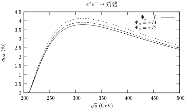
Figure 2: Total cross section for $e^{+}e^{-}\to{\tilde{\chi}^{0}}_{1}{\tilde{\chi}^{0}}_{2}$ in fb. We fix $\tan\beta=10$, $P_{e}=-0.8$, and $\bar{P}_{e}=0.6$.

In order to probe the stau sector through the subsequent decay of ${\tilde{\chi}^{0}}_{2}\to{\tilde{\tau}}_{1}^{\pm}\tau^{\mp}$ following $e^{+}e^{-}\to{\tilde{\chi}^{0}}_{1}{\tilde{\chi}^{0}}_{2}$, the first question is whether the ${\tilde{\chi}^{0}}_{1}{\tilde{\chi}^{0}}_{2}$ production cross section is sufficiently large. In Fig. 2, we show $\sigma_{tot}(e^{+}e^{-}\to{\tilde{\chi}^{0}}_{1}{\tilde{\chi}^{0}}_{2})$ as a function of $\sqrt{s}$ with $\tan\beta=10$ and $\Phi_{1}=0$. The beam polarizations are set as $P_{L}=-0.8$ and $\bar{P}_{L}=0.6$, which maximizes the cross section if $|P_{L}|\leq 0.8$ and $|\bar{P}_{L}|\leq 0.6$. The same choice of beam polarization minimizes the ${\tilde{\tau}}_{1}$ pair background, if $\widetilde{m}_{R}<\widetilde{m}_{L}$ as expected in most SUSY models. The gaugino mass unification relation $|M_{1}|=(5/3)t^{2}_{W}M_{2}$ with $\Phi_{1}=0$ is employed. For $\Phi_{\mu}=0$, the parameters are set as

$$M_{1}=85~{}\mathrm{GeV},\quad|\mu|=200~{}\mathrm{GeV}\,.$$ (28)

For $\Phi_{\mu}=\pi/4$ and $\pi/2$, parameters are chosen to yield the same neutralino mass spectrum as the parameter set Eq. (28), i.e.,

$$m_{{\tilde{\chi}^{0}}_{1}}=76\pm 0.1~{}\mathrm{GeV},\quad m_{{\tilde{\chi}^{0}}_{2}}=132\pm 0.1~{}\mathrm{GeV},\quad m_{{\tilde{\chi}^{0}}_{3}}>200~{}\mathrm{GeV}\,.$$ (29)

For given neutralino masses, a large phase $\Phi_{\mu}$ slightly increases the total cross section. Since the current expectation for the annual luminosity of the future linear collider is about 1000 fb^-1, we have a few thousands events.

4.3 Neutralino polarization vector

The neutralino polarization contains further information especially on the chiral structure of the neutralinos. The polarization vector $\vec{\cal P}^{i}=({\cal P}_{T}^{i},{\cal P}_{N}^{i},{\cal P}_{L}^{i})$ of the neutralino $\tilde{\chi}^{0}_{i}$ is defined in its rest frame. The component ${\cal P}_{L}^{i}$ is parallel to the $\tilde{\chi}^{0}_{i}$ flight direction in the $e^{+}e^{-}$ c.m. frame, ${\cal P}_{T}^{i}$ is in the production plane, which we take to be the $(x,z)$ plane, and ${\cal P}_{N}^{i}$ is normal to the production plane, i.e. in $y$ direction. An explicit calculation gives

$${\cal P}^{i}_{L,T,N}=\frac{\xi\,(1-P_{L}\overline{P}_{L})+(P_{L}-\overline{P}_{L})}{(1-P_{L}\overline{P}_{L})+\xi\,(P_{L}-\overline{P}_{L})}\cdot\frac{\Delta_{L,T,N}}{\Sigma_{U}}\,,$$ (30)

where $\xi$ and $\Sigma_{U}$ have been introduced in Eq.(26). The coefficients $\Delta$ are

$$\Delta_{L}=\phantom{-}4|D_{Z}|^{2}(\alpha^{2}_{R}+\alpha^{2}_{L})\cos\Theta_{i}\left[(1-\mu^{2}_{i}-\mu^{2}_{j})\,|Z_{ij}|^{2}-2\mu_{i}\mu_{j}\,\Re{\rm e}(Z^{2}_{ij})\right],$$

$$\Delta_{T}=-4|D_{Z}|^{2}(\alpha^{2}_{R}+\alpha^{2}_{L})\sin\Theta_{i}\left[(1-\mu^{2}_{i}+\mu^{2}_{j})\mu_{i}\,|Z_{ij}|^{2}-(1+\mu^{2}_{i}-\mu^{2}_{j})\mu_{j}\,\Re{\rm e}(Z^{2}_{ij})\right],$$

$$\Delta_{N}=-4|D_{Z}|^{2}(\alpha^{2}_{R}+\alpha^{2}_{L})\sin\Theta_{i}\hskip 1.42262pt\lambda^{1/2}\mu_{j}\,\Im{\rm m}(Z^{2}_{ij})\,.$$ (31)

Since $\xi=-0.147$ is small, a sizable neutralino polarization is only possible in the presence of large beam polarization. The measurement of the neutralino normal polarization is crucial to probe $\Im{\rm m}(Z^{2}_{ij})$.

Figure 3: Polarization vector components of ${\tilde{\chi}^{0}}_{2}$ as a function of $\cos\Theta_{i}$. We set $\sqrt{s}=300$ GeV, $M_{1}=85$ GeV, $|\mu|=200$ GeV, $\tan\beta=10$, $\Phi_{1}=\Phi_{\mu}=\pi/4$, $P_{L}=-0.8$ and $\bar{P}_{L}=0.6$.

In Fig. 3 we present the polarization vector of ${\tilde{\chi}^{0}}_{2}$ as a function of $\cos\Theta_{i}$ with $\Phi_{1}=\Phi_{\mu}=\pi/4$. The sizable beam polarizations $P_{L}=-0.8$ and $\bar{P}_{L}=0.6$ do generate a substantial polarization of the neutralino. We will see in the next Section that non–vanishing polarization of the neutralino ${\tilde{\chi}^{0}}_{2}$ is essential for measuring the CP-violating phase $\phi_{\tilde{\tau}}$ in the stau sector.

5 Decay of the stau and neutralino

5.1 Stau decays

The decay distribution of the stau decay ${{\tilde{\tau}}}^{\mp}_{a}\rightarrow\tau^{\mp}\tilde{\chi}^{0}_{i}$ and the polarization 4–vector of the final tau lepton in the rest frame of the tau slepton are given by

$$\frac{d\Gamma_{\mp}}{d\Omega^{*}_{1}}=\frac{g^{2}\,m_{\tilde{\tau}_{a}}\,\lambda^{1/2}}{64\,\pi^{2}}\,(|Q^{R}_{ia}|^{2}+|Q^{L}_{ia}|^{2})\,\left[1-\frac{m^{2}_{\tau}}{m^{2}_{\tilde{\tau}_{a}}}-\frac{m^{2}_{\tilde{\chi}^{0}_{i}}}{m^{2}_{\tilde{\tau}_{a}}}\,-2\frac{m_{\tau}m_{\tilde{\chi}^{0}_{i}}}{m^{2}_{\tilde{\tau}_{a}}}\,{\cal A}^{ia}_{T}\right]\,,$$ (32)

$${\cal P}^{\tau^{\mp}}_{\mu}=\mp\frac{{\cal A}^{ia}_{L}}{1-2m_{\tau}m_{\tilde{\chi}^{0}_{i}}/(m^{2}_{\tilde{\tau}_{a}}-m^{2}_{\tau}-m^{2}_{\tilde{\chi}^{0}_{i}})\,{\cal A}^{ia}_{T}}\,\left(\frac{m_{\tau}\,q_{i\mu}}{k_{1}\cdot q_{i}}-\frac{k_{1\mu}}{m_{\tau}}\right),$$ (33)

where $d\Omega^{*}_{1}=d\cos\theta^{*}_{1}d\phi^{*}_{1}$ is the solid angle of the tau lepton in the ${\tilde{\tau}}_{a}$ rest frame, $k_{1}$ and $q_{i}$ are the 4–momenta of the tau lepton $\tau^{\mp}$ and the neutralino $\tilde{\chi}^{0}_{i}$, and the phase space factor $\lambda=\lambda(1,m^{2}_{\tau}/m^{2}_{{\tilde{\tau}}_{a}},m^{2}_{\tilde{\chi}^{0}_{i}}/m^{2}_{{\tilde{\tau}}_{a}})$. Expressions for the $Q^{L,R}_{ia}$ have been given in Eq. (3.3). For the sake of convenience, we introduce three tau polarization asymmetries:

$${{\mathcal{A}}}_{L}^{ia}=\frac{|Q^{R}_{ia}|^{2}-|Q^{L}_{ia}|^{2}}{|Q^{R}_{ia}|^{2}+|Q^{L}_{ia}|^{2}},\quad{{\mathcal{A}}}_{T}^{ia}=\frac{2\hskip 1.42262pt\Re{\rm e}(Q^{R}_{ia}Q^{L*}_{ia})}{|Q^{R}_{ia}|^{2}+|Q^{L}_{ia}|^{2}},\quad{{\mathcal{A}}}_{N}^{ia}=\frac{2\hskip 1.42262pt\Im{\rm m}(Q^{R}_{ia}Q^{L*}_{ia})}{|Q^{R}_{ia}|^{2}+|Q^{L}_{ia}|^{2}}\,.$$ (34)

The average polarization of the $\tau$ lepton can be measured through $\tau$ lepton decays within the detector [26, 27]. Eq.(33) shows that it is purely longitudinally polarized; its degree of polarization is given by

$${\cal P}^{\tau^{\mp}}_{L}=\pm\frac{\lambda^{1/2}(m^{2}_{\tilde{\tau}_{a}},m^{2}_{\tau},m^{2}_{\tilde{\chi}^{0}_{i}})\,{\cal A}^{ia}_{L}}{m^{2}_{\tilde{\tau}_{a}}-m^{2}_{\tau}-m^{2}_{\tilde{\chi}^{0}_{i}}-2m_{\tau}m_{\tilde{\chi}^{0}_{i}}\,{\cal A}^{ia}_{T}}\quad\rightarrow\quad\pm\,{\cal A}^{ia}_{L}\ \ {\rm for}\ \ m_{\tilde{\tau}_{a}}\gg m_{\tau}\,.$$ (35)

In the rest frame of the stau lepton the decay distribution (32) is isotropic, as in all 2–body decays of scalar particles. The degree of longitudinal polarization (35) is constant over phase space, depending only on the couplings $Q^{L,R}_{ia}$. The magnitude of ${\cal P}^{\tau^{\pm}}_{L}$ depends not only on the stau mixing but also on the neutralino mixing as shown in Eq. (3.3). Since the gaugino interaction with (s)fermions preserves chirality while the higgsino interaction flips chirality, ${\cal P}^{\tau^{\pm}}_{L}$ is sensitive to the $\tau$ Yukawa coupling [21]. Note that $\tau$ mass effects, which have been neglected in refs.[21, 22, 17], introduce some dependence of ${\cal P}_{L}^{\tau}$ on the phase $\phi_{\tilde{\tau}}$, via ${\cal A}_{T}^{ia}$. However, this dependence is almost always too weak to allow a measurement of this phase through ${\tilde{\tau}}_{1}\rightarrow{\tilde{\chi}^{0}}_{1}\tau$ decays. Not only is $m_{\tau}m_{{\tilde{\chi}^{0}}_{1}}\ll m^{2}_{{\tilde{\tau}}_{a}}-m^{2}_{{\tilde{\chi}^{0}}_{1}}-m^{2}_{\tau}$ unless $m_{{\tilde{\chi}^{0}}_{1}}$ is very close to $m_{{\tilde{\tau}}_{a}}$, the coefficient ${\cal A}_{T}^{11}$ is usually also significantly smaller in magnitude than 1.

Let us consider some limiting cases of the ${\tilde{\tau}}_{1}\to{\tilde{\chi}^{0}}_{1}\tau$ decay in the limit $m_{{\tilde{\tau}}_{1}}\gg m_{\tau}$, involving the couplings $Q^{R,L}_{11}$. If the lightest neutralino is a pure Bino, the degree of longitudinal polarization of the tau lepton becomes

$${\mathcal{P}}_{\tau}({\tilde{\tau}}_{1}\to\widetilde{B}\tau)=\frac{4\sin^{2}\theta_{\tilde{\tau}}-\cos^{2}\theta_{\tilde{\tau}}}{4\sin^{2}\theta_{\tilde{\tau}}+\cos^{2}\theta_{\tilde{\tau}}}\,,$$ (36)

which has some dependence on the stau mixing angle. If the lighter stau is right-handed, we have

$${\mathcal{P}}_{\tau}({\tilde{\tau}}_{R}\to{\tilde{\chi}^{0}}_{1}\tau)=\frac{2\hskip 1.42262ptt_{W}^{2}|N_{11}|^{2}-Y_{\tau}^{2}|N_{13}|^{2}}{2\hskip 1.42262ptt_{W}^{2}|N_{11}|^{2}+Y_{\tau}^{2}|N_{13}|^{2}}\,,$$ (37)

where $Y_{\tau}=m_{\tau}/(\sqrt{2}m_{W}\cos\beta)$ is the $\tau$ Yukawa coupling divided by the $SU(2)$ gauge coupling. This will deviate significantly from unity only if $\tan\beta$ is large, so that $Y_{\tau}$ becomes comparable to the $U(1)_{Y}$ gauge coupling, and the LSP has a significant higgsino component. Since in most models, including the numerical examples we present below, the LSP is indeed Bino–like and ${\tilde{\tau}}_{1}$ is dominantly ${\tilde{\tau}}_{R}$ (i.e. $\theta_{\tilde{\tau}}$ is near $-\pi/2$), the polarization of $\tau^{-}$ from ${\tilde{\tau}}_{1}^{-}$ decay is usually quite close to $+1$, with little dependence on SUSY parameters (within the ranges allowed by the model) [28]. Measuring this polarization can thus test this (large) class of models, but is often not very useful for determining parameters.

5.2 Neutralino decays

We are interested in the following neutralino production and decay process:

Since the spin-$1/2$ neutralino is polarized through its production as described in Sec. 4.3, non–trivial spin correlations are generated between the decaying neutralino and the tau lepton produced in the first step of ${\tilde{\chi}^{0}}_{i}$ decay. In order to describe the decay distribution and tau polarization, we define a “starred” coordinate system, where the $(x^{*},z^{*})$ plane is still the production plane of the neutralino pair, but the neutralino ${\tilde{\chi}^{0}}_{i}$ momentum points along the $z^{*}$ axis. The “starred” set of axes is thus related to the coordinate system used in Sec. 4 through a rotation around the $y=y^{*}$ axis by the production angle $\Theta_{i}$. In this coordinate system, the polarization vector of the neutralino $\tilde{\chi}^{0}_{i}$ is $\vec{P}^{i}=({\cal P}^{i}_{T},{\cal P}^{i}_{N},{\cal P}^{i}_{L})$ in the rest frame of the neutralino. The expressions for the polarization components are given in Eqs. (30) and (4.3).

The angular distribution and the polarization vector of the $\tau$ lepton from ${\tilde{\chi}^{0}}_{i}$ decay is given in terms of the polar and azimuthal angles $\theta^{*}_{2}$ and $\phi^{*}_{2}$ of the $\tau$ momentum direction with respect to the neutralino momentum direction in the rest frame of the neutralino by

$$\frac{d\Gamma_{\mp}}{d\Omega^{*}_{2}}=\frac{g^{2}\lambda^{1/2}\,E_{\tau}}{64\,\pi^{2}}\,\left(|Q^{R}_{ia}|^{2}+|Q^{L}_{ia}|^{2}\right)\,\left[1+\mu_{\tau}{{\mathcal{A}}}^{ia}_{T}\pm\beta_{\tau}{{\mathcal{A}}}^{ia}_{L}\vec{\cal P}^{i}\cdot\hat{s}^{*}_{3}\right]\,,$$ (38)

$${\cal P}^{\tau^{\mp}}_{L}=\frac{\pm\beta_{\tau}{{\mathcal{A}}}^{ia}_{L}+(1+\mu_{\tau}{{\mathcal{A}}}^{ia}_{T})(\vec{\mathcal{P}}^{i}\cdot\hat{s}^{*}_{3})}{1+\mu_{\tau}{{\mathcal{A}}}^{ia}_{T}\pm\beta_{\tau}{{\mathcal{A}}}^{ia}_{L}(\vec{\cal P}^{i}\cdot\hat{s}^{*}_{3})}\,,$$

$${\cal P}^{\tau^{\mp}}_{T}=\frac{(\mu_{\tau}+{{\mathcal{A}}}^{ia}_{T})\,(\vec{\cal P}^{i}\cdot\hat{s}^{*}_{1})-\beta_{\tau}{{\mathcal{A}}}^{ia}_{N}\,(\vec{\cal P}^{i}\cdot\hat{s}^{*}_{2})}{1+\mu_{\tau}{{\mathcal{A}}}^{ia}_{T}\pm\beta_{\tau}{{\mathcal{A}}}^{ia}_{L}(\vec{\cal P}^{i}\cdot\hat{s}^{*}_{3})}\,,$$

$${\cal P}^{\tau^{\mp}}_{N}=\frac{(\mu_{\tau}+{{\mathcal{A}}}^{ia}_{T})\,(\vec{\cal P}^{i}\cdot\hat{s}^{*}_{2})+\beta_{\tau}{{\mathcal{A}}}^{ia}_{N}\,(\vec{\cal P}^{i}\cdot\hat{s}^{*}_{1})}{1+\mu_{\tau}{{\mathcal{A}}}^{ia}_{T}\pm\beta_{\tau}{{\mathcal{A}}}^{ia}_{L}(\vec{\cal P}^{i}\cdot\hat{s}^{*}_{3})}\,.$$ (39)

Here,

$$E_{\tau}=\frac{m_{{\tilde{\chi}^{0}}_{i}}}{2}\left(1+\frac{m_{\tau}^{2}}{m_{{\tilde{\chi}^{0}}_{i}}^{2}}-\frac{m_{{\tilde{\tau}}_{a}}^{2}}{m_{{\tilde{\chi}^{0}}_{i}}^{2}}\right)$$ (40)

is the energy of the $\tau$ in the ${\tilde{\chi}^{0}}_{i}$ rest frame, $\mu_{\tau}=m_{\tau}/E_{\tau}$, $\lambda^{1/2}\equiv\lambda^{1/2}(1,m^{2}_{{\tilde{\tau}}_{a}}/m^{2}_{{\tilde{\chi}^{0}}_{i}},m^{2}_{\tau}/m^{2}_{{\tilde{\chi}^{0}}_{i}})$, and the tau lepton speed $\beta_{\tau}$ is given by $\beta_{\tau}=\lambda^{1/2}/\left[1-(m^{2}_{{\tilde{\tau}}_{a}}-m^{2}_{\tau})/m^{2}_{{\tilde{\chi}^{0}}_{i}}\right]$. Finally, the three unit vectors $\hat{s}^{*}_{1,2,3}$ are defined by

$$\hat{s}^{*}_{1} = (\cos\theta^{*}_{2}\cos\phi^{*}_{2}\,,\cos\theta^{*}_{2}\sin\phi^{*}_{2}\,,-\sin\theta^{*}_{2})\,,$$

$$\hat{s}^{*}_{2} = (-\sin\phi^{*}_{2}\,,\cos\phi^{*}_{2}\,,0)\,,$$

$$\hat{s}^{*}_{3} = (\sin\theta^{*}_{2}\cos\phi^{*}_{2}\,,\sin\theta^{*}_{2}\sin\phi^{*}_{2}\,,\cos\theta^{*}_{2})\,.$$ (41)

Note that ${\cal P}^{\tau^{\mp}}_{T},{\cal P}^{\tau^{\mp}}_{N},{\cal P}^{\tau^{\mp}}_{L}$ are the polarization components of the $\tau$ polarization vector along the $\hat{s}^{*}_{1},\hat{s}^{*}_{2},\hat{s}^{*}_{3}$ directions, respectively. Combining the three polarization components leads to the $\tau$ polarization 3–vector

$$\vec{\cal P}^{\tau^{\mp}}=\frac{(\mu_{\tau}+{\cal A}^{ia}_{T})\,\vec{\cal P}^{i}+\left[(1-\mu_{\tau})(1-{\cal A}^{ia}_{T})\,(\vec{\cal P}^{i}\cdot\hat{s}^{*}_{3})\pm\beta_{\tau}{\cal A}^{ia}_{L}\right]\hat{s}^{*}_{3}-\beta_{\tau}{\cal A}^{ia}_{N}\,(\vec{\cal P}^{i}\times\hat{s}^{*}_{3})}{1+\mu_{\tau}{{\mathcal{A}}}^{ia}_{T}\pm\beta_{\tau}{{\mathcal{A}}}^{ia}_{L}(\vec{\cal P}^{i}\cdot\hat{s}^{*}_{3})}\,.$$ (42)

The polarization 4–vector of the tau lepton in the neutralino rest frame can be obtained by applying a Lorentz boost along the $\hat{s}^{*}_{3}$ direction with the tau lepton speed $\beta_{\tau}$ to the 4–vector $(0,\vec{\cal P}^{\tau^{\mp}})$.

In the present work we will focus on the decay ${\tilde{\chi}^{0}}_{2}\to\tau^{\mp}{\tilde{\tau}}^{\pm}_{1}$. If the ${\tilde{\chi}^{0}}_{2}$ is unpolarized ($\vec{\cal P}^{i}=0$), only the polarization asymmetry ${{\mathcal{A}}}_{L}^{21}$ defined in the first Eq.(34) can be determined by measuring the longitudinal polarization of the tau lepton. Some limiting cases are:

$${\mathcal{A}}_{L}^{21}({\tilde{\chi}^{0}}_{2}=\widetilde{W}^{3})\!\!\! = \!\!\!-1\,,$$ (43)

$${\mathcal{A}}_{L}^{21}({\tilde{\chi}^{0}}_{2}=\widetilde{H}_{1}^{0})\!\!\! = \!\!\!\cos 2\theta_{\tilde{\tau}}\,,$$

$${\mathcal{A}}_{L}^{21}({\tilde{\tau}}_{1}={\tilde{\tau}}_{R})\!\!\! = \!\!\!\frac{2\hskip 1.42262pt|N_{21}|^{2}\hskip 1.42262ptt_{W}^{2}-Y_{\tau}^{2}|N_{23}|^{2}}{2\hskip 1.42262pt|N_{21}|^{2}\hskip 1.42262ptt_{W}^{2}+Y_{\tau}^{2}|N_{23}|^{2}}\,.$$

The GUT relation $M_{1}\simeq 0.5M_{2}$ suppresses the value of $|N_{21}|$ in most of the parameter space, but for $|\mu|>M_{2}$, $|N_{23}|$ is also suppressed. Even a small ${\tilde{\tau}}_{L}$ component in ${\tilde{\tau}}_{1}$ can therefore change ${\mathcal{A}}_{L}^{21}$ significantly, making it a far more sensitive probe of SUSY parameters than ${\mathcal{A}}_{L}^{11}$.

If the polarization of the neutralino ${\tilde{\chi}^{0}}_{2}$ is sizable, which is possible only with the longitudinal polarization of the $e^{\pm}$ beams, ${\mathcal{A}}_{T}^{21}$ and ${\mathcal{A}}_{N}^{21}$ become measurable. The explicit expression of the numerator of ${\mathcal{A}}_{N}^{21}$ is

$$\Im m(Q^{R}_{21}Q^{L*}_{21})\!\! = \!\!\phantom{-}\sqrt{2}\,t_{W}Y_{\tau}\sin^{2}\theta_{\tilde{\tau}}\Im m(N^{*}_{21}N^{*}_{23})$$

$$-({Y_{\tau}}/{\sqrt{2}}\,)\cos^{2}\theta_{\tilde{\tau}}\Im m(N^{*}_{23}(N^{*}_{22}+N^{*}_{21}t_{W}))$$

$$-t_{W}\sin\theta_{\tau}\cos\theta_{\tilde{\tau}}\Im m(N^{*}_{21}(N^{*}_{22}+N^{*}_{21}t_{W})e^{i\phi_{\tilde{\tau}}})$$

$$+Y_{\tau}^{2}\sin\theta_{\tau}\cos\theta_{\tilde{\tau}}\Im m(N^{*}_{23}N^{*}_{23}e^{-i\phi_{\tilde{\tau}}})\,.$$

$\Re e(Q^{R}_{21}Q^{L*}_{21})$ is the same with $\Im m$ replaced by $\Re e$. The stau CP violating phase $\phi_{\tilde{\tau}}$ is present in the last two terms of Eq. (5.2). Note that these terms are non–zero only in the presence of nontrivial ${\tilde{\tau}}_{L}-{\tilde{\tau}}_{R}$ mixing. This is not surprising, since $\phi_{\tilde{\tau}}$ is associated with the off–diagonal elements of the stau mixing matrix (6). These two terms thus increase with $\tan\beta$; this increase is particularly rapid for the last term, due to the factor $Y_{\tau}^{2}$, but this term is important only for $\tan\beta>20$. On the other hand, if the $U(1)_{Y}$ gaugino mass is real, which is true in our convention if gaugino mass unification also holds for their phases, the first two terms in Eq.(5.2) are proportional to $\sin 2\beta$, i.e. they become small as $\tan\beta$ becomes large. Finally, recall that ${\tilde{\chi}^{0}}_{1,2}$ have to have significant higgsino components in order to obtain a sizable ${\tilde{\chi}^{0}}_{1}{\tilde{\chi}^{0}}_{2}$ production cross section, see Eq.(25). Therefore the necessary conditions for our process to be sensitive to the phase $\phi_{\tilde{\tau}}$ are:

• sizable mixing $\theta_{\tilde{\tau}}$ in the stau sector, which is helped by large $\tan\beta$;

• sizable mixing between gauginos and higgsinos, which requires $|\mu|$ to be not too much larger than $M_{2}$.

5.3 Numerical results of tau polarization asymmetries

Before presenting numerical results of the tau polarization asymmetries for a sample parameter set, some discussions of experimental issues are in order here. Since the final state consists of two tau leptons with two LSP’s, the first question is how to determine which $\tau$ lepton comes from the primary ${\tilde{\chi}^{0}}_{2}$ decay. For example, the negatively charged $\tau^{-}$ can be produced through the following two decay channels:

Decay II : $${\tilde{\chi}^{0}}_{2}\to{\tilde{\tau}}_{1}^{+}\tau^{-}\quad\hbox{followed by}\quad{\tilde{\tau}}_{1}^{+}\to{\tilde{\chi}^{0}}_{1}\tau^{+},$$ (45)

Decay II : $${\tilde{\chi}^{0}}_{2}\to{\tilde{\tau}}_{1}^{-}\tau^{+}\quad\hbox{followed by}\quad{\tilde{\tau}}_{1}^{-}\to{\tilde{\chi}^{0}}_{1}\tau^{-}.$$ (46)

If these two processes are indistinguishable, a substantial reduction of the efficiency is inevitable; recall that the (almost purely longitudinal) polarization of the $\tau$ produced in ${\tilde{\tau}}$ decay depends only very weakly on $\phi_{\tilde{\tau}}$.

In the rest frame of the ${\tilde{\chi}^{0}}_{2}$, the $\tau^{-}$ energy for Decay I is given by Eq.(40) with $i=2,\,a=1$, whereas for Decay II it is distributed over

$$\hbox{{Decay II : }}E_{\tau^{-}}\in\left[\gamma_{{\tilde{\tau}}_{1}}E^{*}_{\tau}-\beta_{{\tilde{\tau}}_{1}}\gamma_{{\tilde{\tau}}_{1}}\left|\vec{p}^{*}_{\tau}\right|,\gamma_{{\tilde{\tau}}_{1}}E^{*}_{\tau}+\beta_{{\tilde{\tau}}_{1}}\gamma_{{\tilde{\tau}}_{1}}\left|\vec{p}^{*}_{\tau}\right|\right]\,.$$ (47)

Here,

$$E^{*}_{\tau}=\frac{m_{{\tilde{\tau}}_{1}}}{2}\left(1+\frac{m_{\tau}^{2}}{m_{{\tilde{\tau}}_{1}}^{2}}-\frac{m_{{\tilde{\chi}^{0}}_{1}}^{2}}{m_{{\tilde{\tau}}_{1}}^{2}}\right)$$ (48)

is the energy of the $\tau$ lepton from ${\tilde{\tau}}_{1}$ decay in the ${\tilde{\tau}}_{1}$ rest frame, $\left|\vec{p}^{*}_{\tau}\right|=\sqrt{E^{*}_{\tau}-m^{2}_{\tau}}$, $\gamma_{{\tilde{\tau}}_{1}}=E_{{\tilde{\tau}}_{1}}/m_{{\tilde{\tau}}_{1}}$, $\beta_{{\tilde{\tau}}_{1}}\gamma_{{\tilde{\tau}}_{1}}=\sqrt{E^{2}_{{\tilde{\tau}}_{1}}/m^{2}_{{\tilde{\tau}}_{1}}-1}$, with

$$E_{{\tilde{\tau}}_{1}}=\frac{m_{{\tilde{\chi}^{0}}_{2}}}{2}\left(1-\frac{m_{\tau}^{2}}{m_{{\tilde{\chi}^{0}}_{2}}^{2}}+\frac{m_{{\tilde{\tau}}_{1}}^{2}}{m_{{\tilde{\chi}^{0}}_{2}}^{2}}\right)$$ (49)

being the energy of ${\tilde{\tau}}_{1}$ in the ${\tilde{\chi}^{0}}_{2}$ rest frame. The boost to the lab frame will broaden the energy distributions from these two decay chains. Nevertheless, for some choices of parameters these ranges do not overlap. In such a situation the question which $\tau$ lepton originates from the ${\tilde{\chi}^{0}}_{2}$ decay can be answered using the energies of two $\tau$ leptons. However, the neutrino(s) produced in the decay of the $\tau$ limit(s) the measurement of the $\tau$ energy. Especially in the decay modes $\tau\to\pi\nu$ and $\tau\to e\nu\nu,\mu\nu\nu$, usually less than half of the $\tau$ energy is visible. On the other hand, in the decays $\tau\to\rho\nu$ or $\tau\to a_{1}\nu$ the substantial mass of the $\rho$ or $a_{1}$ meson enhances the visible energy of the $\tau$. Moreover, these decay modes are known to be useful to measure the tau polarization [26, 27].

As remarked earlier, the situation is cleanest if the two $\tau$ energy distributions show little or no overlap even after the boost to the lab frame. One safe case is when $m_{{\tilde{\tau}}_{1}}$ is close to either $m_{{\tilde{\chi}^{0}}_{1}}$ or $m_{{\tilde{\chi}^{0}}_{2}}$. In this case the signal usually has one rather hard and one rather soft $\tau$ so that the overlap of two $\tau$ energy distributions is not serious. Moreover this signal is easy to distinguish from the possible background process $e^{+}e^{-}\to{\tilde{\tau}}_{1}^{\pm}{\tilde{\tau}}_{1}^{\mp}$ followed by ${\tilde{\tau}}_{1}^{\pm}\to\tau^{\pm}{\tilde{\chi}^{0}}_{1}$ which tends to have either two soft tau’s (if $m_{\tilde{\tau}}$ is close to $m_{{\tilde{\chi}^{0}}_{1}}$), or two hard ones (if $m_{\tilde{\tau}}$ is close to $m_{{\tilde{\chi}^{0}}_{2}}$).

The second issue is the measurement of $\tau$ polarization, which is analyzed through its decay distributions with the decay modes $\tau\to\pi\nu,~{}\rho\nu,~{}a_{1}\nu,~{}\mu\nu\bar{\nu},~{}e\nu\bar{\nu}$. The $\tau\to\pi\nu$ decay mode is useful for determining the $\tau$ polarization only if the $\tau$ energy is known, which is the case in $e^{+}e^{-}\to\tau^{+}\tau^{-}$ production studied at LEP, but not in our case. We consider only the $\rho\nu$ and $a_{1}\nu$ final states with the combined branching ratio of about 34%: The energy distribution of $\rho$ or $a_{1}$ decay products can determine the $\rho$ or $a_{1}$ polarization which can specify, in turn, the $\tau$ polarization [26, 27]. Unfortunately the efficiency of the $\tau$ transverse polarization measurement is usually smaller than that of the $\tau$ longitudinal polarization [29], and is further reduced as the $\tau$ energy increases. Since the $\tau^{-}$ energy is approximately proportional to the mass difference between ${\tilde{\chi}^{0}}_{2}$ and ${\tilde{\tau}}_{1}$, the following mass spectrum is best suited to clearly probe ${\mathcal{A}}_{T,N}$:

The final issue is how to fix the parameters in the current situation without a single signal of supersymmetric particles. Eventually we want to study the $\phi_{\tilde{\tau}}$-dependence of ${\mathcal{A}}^{21}_{L,T,N}$. Varying the phase $\phi_{\tilde{\tau}}$ (through the phases $\Phi_{\mu}$ and/or $\Phi_{A}$) while keeping all the other fundamental parameters the same leads to different mass spectra in the neutralino and stau sectors. This is not reasonable, since most likely these masses will be measured earlier than the polarization observables we are considering. The neutralino and stau sector is determined by the parameters of Eq.(1), where the GUT relation $|M_{1}|=(5/3)t_{W}^{2}M_{2}$ is assumed. As noted earlier, $\widetilde{m}_{R}$ is expected to be smaller than $\widetilde{m}_{L}$ since ${\tilde{\tau}}_{R}$ has no $SU(2)$ interactions. For definiteness, we fix

$$\tan\beta=10,\quad\Phi_{1}=0,\quad|A_{\tau}|=1~{}\mathrm{TeV}\,.$$ (50)

We vary all the other parameters. Considering the optimal scenario for probing $\phi_{\tilde{\tau}}$ as discussed above, we fix the neutralino and stau mass spectrum and stau mixing angle as follows:

$$m_{{\tilde{\chi}^{0}}_{1}} = 80\pm 0.5~{}\mathrm{GeV},\quad m_{{\tilde{\chi}^{0}}_{2}}=140\pm 0.5~{}\mathrm{GeV},\quad m_{{\tilde{\chi}^{0}}_{3}}=225\pm 5~{}\mathrm{GeV},\quad$$ (51)

$$m_{{\tilde{\tau}}_{1}} = 130\pm 1~{}\mathrm{GeV},\quad m_{{\tilde{\tau}}_{2}}=210\pm 1~{}\mathrm{GeV},\quad\theta_{\tilde{\tau}}=-1.5\pm 0.02\,.$$

This constrains the mass parameters [in GeV]:

$$M_{1}\in[81.8,88.3],\quad|\mu|\in[206,220],\quad\widetilde{m}_{R}\in[122.5,128.5],\quad\widetilde{m}_{L}-\widetilde{m}_{R}\in[72,82.5]\,,$$ (52)

while the CP–violating phase $\phi_{\tilde{\tau}}$ is completely unconstrained.

Figure 4: The longitudinal polarization asymmetry of $\tau^{-}$ from Decay I. Parameters are as in Eqs.(50) and (51).

Figure 5: The transverse and normal polarization asymmetries of $\tau^{-}$ from Decay I. Parameters are as in Eqs.(50) and (51).

Figure 4 presents the longitudinal polarization asymmetry of the $\tau^{-}$ lepton produced in Decay I, while Fig. 5 presents its transverse and normal polarization asymmetries. Here ${\mathcal{A}}_{L,T,N}\equiv{\mathcal{A}}_{L,T,N}^{21}$. The spread of the points for fixed $\phi_{\tilde{\tau}}$ is attributed to our choice of SUSY scenario by fixing the neutralino and stau mass spectra within finite error margins, rather than fixing the fundamental SUSY parameters. As can be seen from Fig. 4, this procedure introduces some dependence of ${\mathcal{A}}_{L}^{21}$ on $\phi_{\tilde{\tau}}$, mostly through the change of the ${\tilde{\chi}^{0}}_{2}$ decomposition. We had seen earlier that this quantity is very sensitive to various SUSY parameters. However, the spread of the points is too large to allow a good measurement of $\phi_{\tilde{\tau}}$. In contrast, Fig. 5 clearly shows that ${\mathcal{A}}_{T}^{21}$ and ${\mathcal{A}}_{N}^{21}$ are quite sensitive to $\phi_{\tilde{\tau}}$. As expected from Eqs.(34), they show complementary behavior: When $|{\mathcal{A}}_{N}|\simeq 1$ (particularly when $Q^{R}_{21}$ is almost real and $Q^{L}_{21}$ almost imaginary or vice versa), ${\mathcal{A}}_{T}$ becomes minimized; when $|{\mathcal{A}}_{T}|\simeq 1$ (particularly when both $Q^{R}_{21}$ and $Q^{L}_{21}$ are almost either real or imaginary) ${\mathcal{A}}_{N}$ becomes minimized.

6 Case studies

In the previous Section we saw that the polarization of the $\tau$ lepton produced in the primary ${\tilde{\chi}^{0}}_{2}$ decay ${\tilde{\chi}^{0}}_{2}\to{\tilde{\tau}}^{\pm}\tau^{\mp}$ depends sensitively on $\phi_{\tilde{\tau}}$ through the polarization asymmetries ${\mathcal{A}}_{T,N}^{21}$. However, these quantities can be directly extracted from the measurable $\tau$ polarization in the lab frame only if the event can be reconstructed completely. In the case at hand this would be true (up to possible discrete ambiguities) if the masses of all participating superparticles were known, and if the $\tau$ energies could be measured. Unfortunately, even in $\tau\to\rho\nu,\,a_{1}\nu$ decays a significant fraction of the $\tau$ energy will usually be carried away by the neutrino, making such an approach impractical.

In this Section we therefore discuss the $\tau$ polarization in the lab frame, as function of kinematical variables that are also defined in the lab frame. To this end we have to boost the $\tau$ 4–momentum, whose spatial component in the “starred” coordinate system points in the direction of the unit vector $\hat{s}_{3}^{*}$ introduced in Eq.(5.2), into the lab frame. In order to describe the behavior of the $\tau$ lepton produced in the second step of the ${\tilde{\chi}^{0}}_{2}$ cascade decay, we have to model ${\tilde{\tau}}_{1}$ decays in the ${\tilde{\tau}}_{1}$ rest frame as described in Sec. 5.1, and again boost it into the lab frame. Altogether we thus have to integrate over five angular variables: the production angle $\Theta_{2}$ introduced in Sec. 4.2, and the angles $\theta_{1}^{*},\,\phi_{1}^{*}$ and $\theta_{2}^{*},\,\phi_{2}^{*}$ describing ${\tilde{\tau}}_{1}\to\tau{\tilde{\chi}^{0}}_{1}$ and ${\tilde{\chi}^{0}}_{2}\to{\tilde{\tau}}_{1}\tau$ decays, respectively. This is done using Monte Carlo methods.

We chose two points in the parameter space defined by Eqs.(50) and (51). Both have

$$\widetilde{m}_{L}=205\ {\rm GeV}\,,\quad\widetilde{m}_{R}=124\ {\rm GeV}\,,\quad|\mu|=215\ {\rm GeV}\,.$$ (53)

Set I conserves CP:

$$\hbox{{Set \phantom{I}I : }}|M_{1}|=87.5\ {\rm GeV}\,,\quad\Phi_{\mu}=0\,,\quad\Phi_{A}=\pi\quad\quad\Rightarrow\phi_{\tilde{\tau}}=\pi\,,$$ (54)

while CP is violated for Set II:

$$\hbox{{Set II : }}|M_{1}|=84.3\ {\rm GeV}\,,\quad\Phi_{\mu}=\frac{\pi}{2}=\Phi_{A}\quad\quad\Rightarrow\phi_{\tilde{\tau}}=\frac{\pi}{2}\,.$$ (55)

Note that $|m_{RL}|$, and hence $\theta_{\tilde{\tau}}$, is the same in both cases, whereas the phase $\phi_{\tilde{\tau}}$ changes. We choose center–of–mass energy $\sqrt{s}=300$ GeV, where the signal cross section is near its maximum, and take $P_{L}=-0.8,\,\overline{P}_{L}=0.6$.

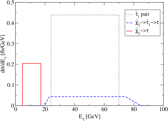
Figure 6: Energy distribution of the “soft” (solid red) and “hard” (dashed blue) $\tau$ lepton from ${\tilde{\chi}^{0}}_{2}$ decay, as well as for the $\tau$ lepton from ${\tilde{\tau}}_{1}$ pair production and decay (dotted black). Parameters are as in Eqs.(50), (53) and (54).

The resulting $\tau$ energy distributions are shown in Fig. 6. The (red) solid curve gives the energy distribution for the “soft” $\tau$ from the primary ${\tilde{\chi}^{0}}_{2}$ decay, whereas the dashed (blue) curve is for the “hard” $\tau$ lepton produced in the second ${\tilde{\chi}^{0}}_{2}$ decay step. As advertised in Sec. 5.3, these two distributions do not overlap. Moreover, the energy distribution from $e^{+}e^{-}\to{\tilde{\tau}}_{1}^{+}{\tilde{\tau}}_{1}^{-}\to\tau^{+}\tau^{-}{\tilde{\chi}^{0}}_{1}{\tilde{\chi}^{0}}_{1}$ (dotted black curve) is also well separated from that of the “soft” $\tau$ lepton from ${\tilde{\chi}^{0}}_{2}$ decay. Note that this last distribution is completely flat, even though Fig. 3, which uses very similar parameters, shows that ${\tilde{\chi}^{0}}_{2}$ can be strongly polarized. The energy of this $\tau$ lepton only depends on $\cos\theta_{2}^{*}$: it will be maximal (minimal) if $\cos\theta_{2}^{*}=+1\ (-1)$. Eq.(38) shows that after integrating over $\phi_{2}^{*}$, the ${\tilde{\chi}^{0}}_{2}$ decay distribution only depends on the longitudinal ${\tilde{\chi}^{0}}_{2}$ polarization ${\cal P}_{L}^{2}$, which according to the first Eq.(4.3) is proportional to $\cos\Theta_{2}$. Integrating over $\cos\Theta_{2}$ will therefore lead to a vanishing average ${\cal P}_{L}^{2}$, and hence to flat energy distributions of the primary ${\tilde{\chi}^{0}}_{2}$ decay products. Since all masses are (essentially) the same for our two sets, Fig. 6 is valid for both of them.

Fig. 7 shows angular distributions of the $\tau$ leptons from Decay I of eq.(47). The (red) solid and (blue) dashed curves show the cross section as function of the cosine of the angle between the $e^{-}$ beam direction and the direction of the soft and hard $\tau$, respectively; the corresponding distributions for Decay II can be obtained by sending $\cos\Theta\rightarrow-\cos\Theta$. The “soft” $\tau$ shows quite a pronounced forward–backward asymmetry. This can again be explained from Eqs.(38) and (4.3). If ${\tilde{\chi}^{0}}_{2}$ goes in forward direction, $\cos\Theta_{2}>0$, we have ${\cal P}_{L}^{2}<0$ (see Fig. 3). Since ${\mathcal{A}}_{L}^{21}>0$, see Fig. 4, this means that the soft $\tau$ will be emitted preferentially in the direction opposite to that of ${\tilde{\chi}^{0}}_{2}$, i.e. in backward direction. On the other hand, if $\cos\Theta_{2}<0$, we have ${\cal P}_{L}^{2}>0$, and the “soft” $\tau$ will be emitted preferentially collinear with ${\tilde{\chi}^{0}}_{2}$, i.e. again in backward direction. The size of this effect depends on ${\mathcal{A}}_{L}^{21}$: Fig. 4 shows a smaller ${\mathcal{A}}_{L}^{21}$ for $\phi_{\tilde{\tau}}=\pi/2$ (Set II), leading to a less pronounced forward–backward asymmetry, as illustrated by the (red) dot–dashed curve. Finally, the (black) dotted curve shows the cross section as function of the cosine of the opening angle between the two $\tau$ leptons. This distribution peaks at small angles, as expected from the discussion at the end of Sec. 2. However, this peak is not very pronounced, since the boost from the ${\tilde{\chi}^{0}}_{2}$ rest frame to the lab frame is not very large. This distribution is the same for Decay I and Decay II.

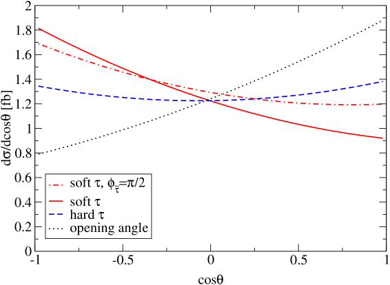
Figure 7: Angular distributions of the $\tau$ leptons from ${\tilde{\chi}^{0}}_{2}{\tilde{\chi}^{0}}_{1}$ production and decay. Parameters are as described in the text.

We know from the discussion of Sec. 5.3 that the main sensitivity to $\phi_{\tilde{\tau}}$ comes from the components of the $\tau$ polarization that are orthogonal to the $\tau$ 3–momentum. In principle, ${\mathcal{A}}_{T}^{21}$ and ${\mathcal{A}}_{N}^{21}$ are equally well suited to determine this phase. However, observation of a CP– or T–odd quantity would clearly be a more convincing proof of CP violation in the stau and/or neutralino sector. Our choice of beam polarization implies that the initial state is not CP self–conjugate. On the other hand, since we are working in Born approximation and are neglecting finite particle width effects, we can replace the T transformation by the so–called naive $\widetilde{T}$ transformation, which reverses the directions of all 3–momenta and spins, but does not exchange initial and final state. Recall, however, that we define the $e^{-}$ beam to go in $+z$ direction, whereas the transverse component of the ${\tilde{\chi}^{0}}_{2}$ 3–momentum defines the $+x$ direction. In our coordinate system a $\widetilde{T}$ transformation therefore amounts to only changing the $y$ components of all 3–momenta and spins; recall that the $y$ axis is the same in the original coordinate system of Sec. 4 and the “starred” system introduced in Sec. 5.2. Practically speaking, the $\widetilde{T}$ conjugate of some kinematic configuration can therefore be obtained by simply sending $\phi_{1}^{*}\rightarrow-\phi_{1}^{*}$ and $\phi_{2}^{*}\rightarrow-\phi_{2}^{*}$. The existence of $\widetilde{T}$, and hence CP, violation is established if some observable takes different values for some configuration and the $\widetilde{T}$ conjugate one. Note that these two configurations result in the same $\tau$ energies; the angular variables whose distributions are shown in Fig. 7 also remain unchanged.

The simplest such observables involve the triple product of three momentum or spin vectors. The triple product of the momenta of the final–state leptons with the incoming $e^{-}$ momentum has been studied in refs.[16]. This observable is sensitive to CP violation in the neutralino sector, but is not sensitive to $\phi_{\tilde{\tau}}$: We saw above that the $\tau$ energy distribution only depends on ${\mathcal{A}}_{L}^{21}$, not on ${\mathcal{A}}_{T,N}^{21}$. Here we therefore study the component of the “soft” $\tau$ polarization that is normal either to the “event” plane defined by the $e^{-}$ beam and the 3–momentum of this $\tau$, or normal to the “$\tau\tau$” plane spanned by the 3–momenta of the two $\tau$’s in the final state. In both cases we also analyze the “transverse” component of the $\tau$ polarization of the “soft” $\tau$ leptons that lies in this plane.

The dependence of the polarization of the soft $\tau$ lepton on its energy is shown in Fig. 8 for Decay I. The (black) dotted and dash–doubledotted curves show the longitudinal polarizations for Set I and Set II, respectively. We see that it is essentially independent of $E_{\tau}$ after integrating over the production angle $\Theta_{2}$. This component is boost–invariant, up to terms of order $m_{\tau}^{2}$. Its average value can thus be computed from Eqs.(38) and (5.2):

$$\langle{\cal P}_{L}^{\tau^{\mp}}\rangle\simeq\pm\frac{\beta_{\tau}{\mathcal{A}}_{L}^{21}}{1+\mu_{\tau}{\mathcal{A}}_{T}^{21}}\,,$$ (56)

which well describes the numerical results of Fig. 8. Note in particular that this component of the polarization has opposite sign for Decay II, where the “soft” $\tau$ is positively charged.

The (blue) dashed and lower solid curves show the transverse polarization in the “event” plane for Set I and Set II, respectively. It clearly mirrors the behavior of ${\mathcal{A}}_{T}^{21}$ shown in Fig. 5, being sizable and negative for $\phi_{\tilde{\tau}}=\pi$, but small for $\phi_{\tilde{\tau}}=\pi/2$. It has some dependence on the $\tau$ energy, reaching its maximal absolute value for some intermediate $E_{\tau}$. This corresponds to small values of $\cos\theta_{2}^{*}$, i.e. $|\sin\theta_{2}^{*}|\simeq 1$, which in turn maximizes the product $\vec{\cal P}^{2}\cdot\hat{s}_{1}^{*}$ that multiplies ${\mathcal{A}}_{T}^{21}$ in the second eq.(5.2); recall from Fig. 3 that ${\cal P}_{L}^{2}$ is the potentially biggest component of $\vec{\cal P}^{2}$. In contrast, the (blue) dot–dashed curve shows that the transverse polarization in the “$\tau\tau$” plane is small even for $\phi_{\tilde{\tau}}=\pi$. We suspect that such a small polarization, of less than 5%, will be very difficult to measure.

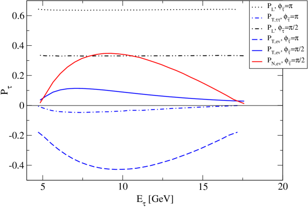
Figure 8: Energy dependence of the components of the polarization vector of the $\tau^{-}$ produced in Decay I. The transverse $T$ and normal $N$ components are defined either with respect to the plane spanned by the $e^{-}$ and $\tau$ 3–momenta (subscript “ev”), or with respect to the plane spanned by the 3–momenta of the two $\tau$ leptons in the final state (subscript “$\tau\tau$”). Phase $\phi_{\tilde{\tau}}=\pi\ (\pi/2)$ refers to parameter Set I (Set II).

The upper (red) solid curve in Fig. 8 shows the $\tau$ polarization normal to the “event” plane for Set II; since this is a T–odd quantity, it vanishes identically for Set I. It again tracks the behavior shown in Fig. 5, being large and positive for $\phi_{\tilde{\tau}}=\pi/2$. Also like ${\cal P}_{T,{\rm ev}}^{\tau}$, it shows a pronounced extremum at intermediate values of $E_{\tau}$. Note that the product $\vec{\cal P}^{2}\cdot\hat{s}_{1}^{*}$, which is maximized in this region of phase space, now multiplies the CP–odd quantity ${\mathcal{A}}_{N}^{21}$ in the last Eq.(5.2). The $\tau$ polarization normal to the “$\tau\tau$” plane (not shown) is always much smaller than that normal to the “event” plane.

Fig. 9 shows the same $\tau$ polarization components as in Fig. 8, as function of the cosine of the angle between the incoming $e^{-}$ and outgoing $\tau$ 3–momenta. We see that the longitudinal $\tau$ polarization depends quite strongly on this angle. A value of $\cos\Theta_{\tau}$ near $-1$ is easiest to achieve if $\cos\Theta_{2}\simeq-1$ and $\cos\theta_{2}^{*}\simeq+1$, which results in $\vec{\cal P}^{2}\cdot\hat{s}_{3}^{*}>0$ after integrating over $\phi_{2}^{*}$, so that both terms in the numerator of the first eq.(5.2) are positive. In contrast, $\cos\Theta_{\tau}\simeq 1$ is most easily achievable if $\cos\Theta_{2}\simeq\cos\theta_{2}^{*}\simeq+1$, which gives a negative product $\vec{\cal P}^{2}\cdot\hat{s}_{3}^{*}$. For parameter Set II, where ${\mathcal{A}}_{L}^{21}$ is smaller, this even leads to negative ${\cal P}^{\tau}_{L}$ in the forward direction. As before, ${\cal P}_{L}^{\tau}$ has to be reversed for Decay II.

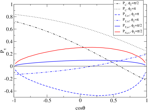
Figure 9: Dependence of the components of the polarization vector of the $\tau^{-}$ produced in Decay I on the cosine of the angle between this $\tau$ and the $e^{-}$ beam. Parameters and notation are as in Fig.8.

The overall behavior of the transverse and normal components defined w.r.t. the “event” plane again follows the behavior of ${\mathcal{A}}_{T}^{21}$ and ${\mathcal{A}}_{N}^{21}$, respectively, as displayed in Fig. 5. We saw above that these components reach their maximal values if $|\sin\theta_{2}^{*}|\simeq 1$, which implies small $\cos\theta_{2}^{*}$ and also the lab system variable $|\cos\Theta_{\tau}|$ well away from unity. On the other hand, we now see that the tranverse $\tau$ polarization defined w.r.t. the “$\tau\tau$” plane can reach up to 20% for parameter Set I, which however is still well below the maximal value of $|{\cal P}_{T,{\rm ev}}^{\tau}|$.

Finally, we also investigated $\vec{\cal P}^{\tau}$ as function of the opening angle between the two $\tau$ leptons in the final state. In all cases we find a very weak dependence on this angle. Note that this angle is independent of the production angle $\Theta_{2}$, and only weakly dependent on the ${\tilde{\chi}^{0}}_{2}$ decay angle $\theta_{2}^{*}$. We saw above that these two variables largely determine the $\tau$ polarization. Integrating over them thus essentially reduces these polarizations to their average values.

7 Summary and Conclusions

In this paper we have investigated associated ${\tilde{\chi}^{0}}_{1}{\tilde{\chi}^{0}}_{2}$ production followed by the two–step decay ${\tilde{\chi}^{0}}_{2}\to{\tilde{\tau}}^{\pm}\tau^{\mp}\to{\tilde{\chi}^{0}}_{1}\tau^{+}\tau^{-}$. We have seen that the components of the $\tau$ lepton produced in the first step of this decay that are orthogonal to the $\tau$ momentum are very sensitive to the CP–odd phase $\phi_{\tilde{\tau}}$ in the stau sector. Much of this sensitivity survives after boosting into the lab frame; the most sensitive region of phase space involves intermediate values of both the $\tau$ energy and its angle with respect to the beam direction. In particular, we found a CP–violating normal component in excess of 30% in certain regions of phase space, if $\phi_{\tilde{\tau}}=\pi/2$. Strong (longitudinal) beam polarization is crucial to find such large CP–violating effects.

Of course, this result depends on the assumptions we made. To begin with, we assumed an “inverted hierarchy” where the first and second generation sfermions are very heavy. This is a conservative assumption in the sense that it reduces our signal cross section by about two orders of magnitude. On the other hand, it removes the otherwise very stringent constraints on CP violation in the neutralino sector, in particular on the phase $\Phi_{\mu}$ of $\mu$. It also implies that the decay mode we are investigating has branching ratio near 100% if ${\tilde{\tau}}_{1}$ lies in between the two neutralinos. Here we analyzed a situation with relatively small neutralino masses, where competing 2–body decay processes ${\tilde{\chi}^{0}}_{2}\to{\tilde{\chi}^{0}}_{1}Z$ or ${\tilde{\chi}^{0}}_{2}\to{\tilde{\chi}^{0}}_{1}h$ are not open; however, for gaugino–like neutralinos (which generally have sizable mass splittings) these competing decays have rather small branching ratios even if they are allowed.

A second important assumption is that ${\tilde{\tau}}_{L}-{\tilde{\tau}}_{R}$ mixing should not be too small. This should be clear, since for vanishing mixing the phase $\phi_{\tilde{\tau}}$ looses its physical meaning. We found that the rather moderate choice $\tan\beta=10$ is quite sufficient for this purpose. This value of $\tan\beta$ is already so large that the neutralino masses and couplings show relatively little sensitivity to the phase $\Phi_{\mu}$. Our CP–odd observable is therefore indeed mostly attributable to the stau sector.

We also assumed that ${\tilde{\tau}}_{1}$ is quite close in mass to ${\tilde{\chi}^{0}}_{2}$. This makes it easy to decide on an event–by–event basis whether ${\tilde{\chi}^{0}}_{2}$ decays into a positive or negative ${\tilde{\tau}}_{1}$, or equivalently, which of the two $\tau$ leptons in the final state is produced in the first step of ${\tilde{\chi}^{0}}_{2}$ decay; note that only this lepton can have sizable transverse and normal polarization components. However, even if no distinction between the two ${\tilde{\chi}^{0}}_{2}$ decay chains was possible, the necessary averaging would only reduce the transverse and normal polarization asymmetries by a factor of 2.

Within the framework of inverted hierarchy models, our main assumption is thus that ${\tilde{\chi}^{0}}_{2}\rightarrow{\tilde{\tau}}_{1}\tau$ 2–body decays are open but decays into ${\tilde{\tau}}_{2}$ are not. If this second decay mode was also open, more decay chains would need to be investigated; if they cannot be distinguished experimentally, one may have to average over them, which could lead to further degradation of the $\tau$ polarization. However, in most SUSY models the region of parameter space where $m_{{\tilde{\tau}}_{2}}<m_{{\tilde{\chi}^{0}}_{2}}$ is rather small. On the other hand, $m_{{\tilde{\tau}}_{1}}>m_{{\tilde{\chi}^{0}}_{2}}$ seems quite feasible. If the competing ${\tilde{\chi}^{0}}_{2}$ 2–body decays are also closed, ${\tilde{\chi}^{0}}_{2}\rightarrow\tau^{+}\tau^{-}{\tilde{\chi}^{0}}_{1}$ would still have a large, often dominant, branching ratio; in many cases virtual ${\tilde{\tau}}$ exchange would give significant contributions [30]. We therefore believe that in this case sizable polarizations that are sensitive to $\phi_{\tilde{\tau}}$ can again be found. If the competing ${\tilde{\chi}^{0}}_{2}$ 2–body decays are open but the decay into ${\tilde{\tau}}_{1}$ is not, ${\tilde{\chi}^{0}}_{2}$ decays would not be a good probe of $\phi_{\tilde{\tau}}$, since the final state of interest would then only receive a very small contribution from virtual ${\tilde{\tau}}$ exchange. However, in this case one may still be able to extract this information from analyses of the decays of heavier neutralinos, which of course would require a somewhat higher beam energy.

We therefore conclude that neutralino decays into $\tau$ pairs offer a good, indeed probably the best, possibility to probe CP violation in the stau sector at $e^{+}e^{-}$ colliders.

Acknowledgements

This work was partially supported by the KOSEF–DFG Joint Research Project No. 20015-111-02-2. In addition, the work of SYC was supported in part by the Korea Research Foundation through the grant KRF-2002-070-C00022 and in part by KOSEF through CHEP at Kyungpook National University. The work of JS is supported by the faculty research fund of Konkuk University in 2003, and partly by Grant No. R02-2003-000-10050-0 from BR of the KOSEF. The work of MD and BG was partially supported by the Deutsche Forschungsgemeinschaft, grant Dr 263.

References

- [1] H.P. Nilles, Phys. Rept. 110 (1984) 1; H. Haber and G. Kane, Phys. Rept. 117 (1985) 75.
- [2] E. Witten, Nucl. Phys. B188, 513 (1981); N. Sakai, Z. Phys. C11, 153 (1981); S. Dimopoulos and H. Georgi, Nucl. Phys. B193, 150 (1981); R.K. Kaul and P. Majumdar, Nucl. Phys. B199. 36 (1982).
- [3] C. Giunti, C. W. Kim and U. W. Lee, Mod. Phys. Lett. A6, 1745 (1991); U. Amaldi, W. de Boer and H. Fürstenau, Phys. Lett. B260, 447 (1991); P. Langacker and M. x. Luo, Phys. Rev. D44, 817 (1991); J. R. Ellis, S. Kelley and D. V. Nanopoulos, Phys. Lett. B260, 131 (1991).
- [4] L. E. Ibáñez and G. G. Ross, Phys. Lett. B110, 215 (1982).
- [5] H. Goldberg, Phys. Rev. Lett. 50, 1419 (1983); J. R. Ellis, J. S. Hagelin, D. V. Nanopoulos, K. A. Olive and M. Srednicki, Nucl. Phys. B238, 453 (1984).
- [6] S. Dimopoulos and D. Sutter, Nucl. Phys. B452, 496 (1995), hep–ph/9504415; H.E. Haber, Nucl. Phys. Proc. Suppl. 62, 469 (1998), hep–ph/9709450.
- [7] A. D. Sakharov, Zh. Éksp. Teor. Fiz. 5, 32 (1967) [JETP Lett. 91B, 24 (1967)].
- [8] Particle Data Group, K. Hagiwara et al., Phys. Rev. D66, 010001 (2002).
- [9] T. Ibrahim and P. Nath, Phys. Rev. D57, 478 (1998), Erratum-ibid. D58 (1998), D60, 019901 (1999), hep–ph/9708456; M. Brhlik, G.J. Good and G.L. Kane, Phys. Rev. D59 115004, (1999), hep–ph/9810457.
- [10] See e.g. F. Gabbiani, E. Gabrielli, A. Masiero and L. Silvestrini, Nucl. Phys. B477, 321 (1996), hep–ph/9604387.
- [11] T. Goto and T. Nihei, Phys. Rev. D59, 115009 (1999), hep–ph/9808255.
- [12] M. Drees, Phys. Rev. D33, 1468 (1986); A.G. Cohen, D.B. Kaplan and A.E. Nelson, Phys. Lett. B388, 588 (1996), hep–ph/9607394; J. A. Bagger, J. L. Feng, N. Polonsky and R. J. Zhang, Phys. Lett. B473, 264 (2000), hep–ph/9911255.
- [13] B. C. Allanach et al., in Proc. of the APS/DPF/DPB Summer Study on the Future of Particle Physics (Snowmass 2001), ed. N. Graf, Eur. Phys. J. C25, 113 (2002), hep–ph/0202233.
- [14] B. Ananthanarayan, G. Lazarides and Q. Shafi, Phys. Rev. D44, 1613 (1991); S. Kelley, J. L. Lopez and D. V. Nanopoulos, Phys. Lett. B274, 387 (1992).
- [15] LEP Higgs Working Group, hep–ex/0107030.
- [16] S.T. Petcov, Phys. Lett. B178, 57 (1986); N. Oshimo, Z. Phys. C41, 129 (1988); Y. Kizukuri and N. Oshimo, Phys. Lett. B249, 449 (1990); S.Y. Choi, H.S. Song and W.Y. Song, Phys. Rev. D61, 075004 (2000), hep–ph/9907474; V.D. Barger, T. Falk, T. Han, J. Jiang, T. Li and T. Plehn, Phys. Rev. D64, 056007 (2001), hep–ph/0101106; A. Bartl, H. Fraas, O. Kittel and W. Majerotto, hep–ph/0308141.
- [17] A. Bartl, T. Kernreiter and O. Kittel, hep–ph/0309340.
- [18] G. A. Blair, W. Porod and P. M. Zerwas, Phys. Rev. D63, 017703 (2001), hep–ph/0007107, and Eur. Phys. J. C27, 263 (2003), hep–ph/0210058.
- [19] T. Tsukamoto, K. Fujii, H. Murayama and M. Yamaguchi, Phys. Rev. D51, 3153 (1995); S.Y. Choi, A. Djouadi, M. Guchait, J. Kalinowski, H.S. Song and P.M. Zerwas, Eur. Phys. J. C14, 535 (2000), hep-ph/0002033.
- [20] S. Y. Choi, J. Kalinowski, G. Moortgat-Pick and P. M. Zerwas, Eur. Phys. J. C22, 563 (2001), Addendum-ibid. C23, 769 (2002), hep–ph/0108117.
- [21] M.M. Nojiri, Phys. Rev. D51, 6281 (1995), hep–ph/9412374; M.M. Nojiri, K. Fujii and T. Tsukamoto, Phys. Rev. D54, 6756 (1996), hep–ph/9606370.
- [22] E. Boos, G. Moortgat-Pick, H. U. Martyn, M. Sachwitz and A. Vologdin, hep–ph/0211040; E. Boos, H. U. Martyn, G. Moortgat-Pick, M. Sachwitz, A. Sherstnev and P. M. Zerwas, Eur. Phys. J. C30, 395 (2003), hep–ph/0303110.
- [23] A. Bartl, H. Eberl, S. Kraml, W. Majerotto and W. Porod, Z. Phys. C73, 469 (1997), hep–ph/9603410; A. Bartl, H. Eberl, S. Kraml, W. Majerotto, W. Porod and A. Sopczak, Z. Phys. C76, 549 (1997), hep–ph/9701336; A. Bartl, H. Eberl, S. Kraml, W. Majerotto and W. Porod, Eur. Phys. J. direct C2, 6 (2000), hep–ph/0002115.
- [24] S.Y. Choi and M. Drees, Phys. Lett. B435, 356 (1998), hep–ph/9805474.
- [25] G. Moortgat-Pick, A. Bartl, H. Fraas and W. Majerotto, Eur. Phys. J. C18, 379 (2000), hep–ph/0007222.
- [26] B.K. Bullock, K. Hagiwara and A.D. Martin, Phys. Rev. Lett. 67, 3055 (1991), and Nucl. Phys. B395, 499 (1993).
- [27] M. Davier, L. Duflot, F. Le Diberder and A. Rouge, Phys. Lett. B306, 411 (1993).
- [28] M. Guchait and D.P. Roy, Phys. Lett. B541, 356 (2002), hep–ph/0205015.
- [29] A. Bartl, T. Kernreiter and W. Porod, Phys. Lett. B538, 59 (2002), hep–ph/0202198.
- [30] H. Baer, C.-. Chen, M. Drees, F. Paige and X. Tata, Phys. Rev. D58, 075008 (1998), hep–ph/9802441; M.M. Nojiri and Y. Yamada, Phys. Rev. D60, 015006 (1999), hep–ph/9902201; A. Djouadi, Y. Mambrini and M. Mühlleitner, Eur. Phys. J. C20, 563 (2001), hep–ph/0104115.