HISKP-TH-03/18

IPNO/DR-03-08/

LPT-ORSAY/03-76

A new analysis of $\pi K$ scattering
from Roy and Steiner type equations

P. Büttiker^a, S. Descotes-Genon^b and B. Moussallam^c

^a Helmholtz-Institut für Strahlen- und Kernphysik,
Universität Bonn, D-53115 Bonn, Germany

^b Laboratoire de Physique Théorique
Université Paris-Sud, F-91406 Orsay, France

^c Institut de Physique Nucléaire
Université Paris-Sud, F-91406 Orsay, France

With the aim of generating new constraints on the OZI suppressed couplings of chiral perturbation theory a set of six equations of the Roy and Steiner type for the $S$- and $P$-waves of the $\pi K$ scattering amplitudes is derived. The range of validity and the multiplicity of the solutions are discussed. Precise numerical solutions are obtained in the range $E\mathrel{\raise 2.58334pt\hbox{$<$}\kern-7.7778pt\lower 2.79857pt\hbox{$\sim$}}1$ GeV which make use as input, for the first time, of the most accurate experimental data available at $E\mathrel{\raise 2.58334pt\hbox{$>$}\kern-7.7778pt\lower 2.79857pt\hbox{$\sim$}}1$ GeV for both $\pi K\to\pi K$ and $\pi\pi\to K\overline{K}$ amplitudes. Our main result is the determination of a narrow allowed region for the two S-wave scattering lengths. Present experimental data below 1 GeV are found to be in generally poor agreement with our results. A set of threshold expansion parameters, as well as sub-threshold parameters are computed. For the latter, a matching with the $SU(3)$ chiral expansion at NLO is performed.

1 Introduction

Scattering amplitudes of pseudo-Goldstone bosons at low energies probe with a unique sensitivity the scalar-source sector of Chiral Perturbation Theory (ChPT) [1, 2]. For instance, recent progress in the domain of $\pi\pi$ scattering has provided valuable information on the $SU(2)$ chiral limit where the masses of the $u,d$ quarks are set to zero. For this purpose, the $\pi\pi$ Roy equations, which have been extensively studied in the past [3, 4, 5], were re-analyzed [6] (in particular, a formulation as a boundary value problem was developped) and solved numerically [6, 7] (see also [8]). These equations constrain the low-energy $\pi\pi$-scattering amplitude by exploiting simultaneously theoretical requirements and data at higher energies. New data on $Kl_{4}$ decays from the E865 experiment [9] could thus be studied with the help of the solutions to the Roy equations and a bound on the coupling constant $\bar{\ell}_{3}$ of the $SU(2)$ chiral Lagrangian [10] was derived for the first time. Constraints on the $SU(2)$ quark condensate were also obtained along similar lines [11].

In a parallel way, scattering amplitudes involving both pions and kaons at very low energy should allow one to unveil features of the $SU(3)$ chiral vacuum, i.e. that in the limit where $m_{u}$, $m_{d}$ and $m_{s}$ vanish. The structure of the $SU(3)$ chiral vacuum is worth studying for its own sake, since $SU(3)$ ChPT provides relations between many low-energy processes involving $\pi$-, $K$- and $\eta$-mesons. In addition, it is interesting to compare $SU(2)$ and $SU(3)$ chiral limits, especially in the scalar sector. A sizable difference between the two limits would indicate that sea-quark effects are particularly significant in the case of the strange quark [12, 13]. In previous works [14, 15] it was shown that the ratio of the pion’s decay constant in $SU(2)$ and $SU(3)$ chiral limits could be determined from a sum rule based on $\pi K$ scattering amplitudes. The deviation of this ratio from 1 would indicate a violation of the large-$N_{c}$ approximation. Let us emphasize that the latter is often relied upon to attribute values to some $O(p^{4})$ couplings arising in the scalar sector of the chiral Lagrangian [2, 16]. Our work is motivated by the desire of determining from $\pi K$-scattering experimental data as many chiral couplings as possible (in principle, five out of the ten independent $O(p^{4})$ couplings of the $SU(3)$ chiral Lagrangian [17, 18]), without relying on the large-$N_{c}$ approximation. In this paper, we provide the first step of this analysis, by deriving the analogue of Roy equations for the $\pi K$ system and solving them numerically. A simple matching with the $SU(3)$ expansion is performed while more detailed comparisons with $SU(2)$ and $SU(3)$ expansions are left for future work. Further motivation for the study of $\pi K$ scattering can be found in refs. [19, 20].

In the case of $\pi\pi$ scattering, Roy observed [21] that general properties of analyticity, unitarity, combined with crossing symmetry, lead to a set of non-linear integral equations that the $S$- and $P$-partial waves must satisfy. A similar program was carried out by Steiner for $\pi N$ scattering [22]. Given experimental input at high energies (typically $E\mathrel{\raise 2.58334pt\hbox{$>$}\kern-7.7778pt\lower 2.79857pt\hbox{$\sim$}}1$ GeV), Roy-Steiner (RS) equations constrain the low-energy behaviour of partial-wave amplitudes. In the present paper, we derive and perform a detailed analysis of a system of RS equations for $\pi K$ scattering. In this case, $s-t$ crossing relates the $\pi K\to\pi K$ and the $\pi\pi\to K\overline{K}$ amplitudes, leading to six coupled equations that involve the four $\pi K$ $S$ and $P$ partial-wave amplitudes $f_{0}^{1/2},\ f_{1}^{1/2},\ f_{0}^{3/2},\ f_{1}^{3/2}$ and the two $\pi\pi\to K\overline{K}$ amplitudes $g_{0}^{0},\ g_{1}^{1}$. Equations of a similar kind have been considered earlier [23, 24, 25]. However, some approximations were invoked in the treatment of these equations and, moreover, no accurate experimental input data were available at that time. Since then, high-statistics production experiments have been performed for both $\pi K\to\pi K$ [26, 27] and $\pi\pi\to K\overline{K}$ amplitudes [28, 29]. These experiments provide the necessary input data for the RS equations with a level of accuracy comparable to the case of $\pi\pi$ scattering. Experimental data at lower energies should also be available in the near future: the FOCUS experiment [30] has demonstrated the feasibility of determining the $\pi K$ $S$-wave phase shifts at energies lower that 1 GeV from the weak decays of D mesons [31], P-wave phase shifts should be measured soon in $\tau$ decays [32] and finally, direct determinations of combinations of $S$-wave scattering lengths are expected from planned experiments on kaonic atoms [33].

The plan of the paper is as follows. After reviewing the notation, we derive the set of RS equations that we intend to solve. The setting is similar to a previous work [25] but we differ in the number of subtractions used in the dispersive representations. We aim here at an optimal use of the energy region where accurate experimental data are available, while avoiding to rely on slowly convergent sum rules. After discussing the domains of validity of such equations, we explain our treatment of the available experimental input and of the asymptotic regions. Next, we start solving the equations. One first eliminates $g_{0}^{0}$ and $g_{1}^{1}$ and the remaining four equations then have a similar structure to the $\pi\pi$ Roy equations such that recent results concerning the multiplicity of the solutions [34, 35] can be exploited. Finally, we turn to the numerical resolution and discuss the resulting constraints on the S-wave scattering lengths. Finally, the $\pi K$ amplitudes near and below threshold are constructed and estimates for the $O(p^{4})$ chiral coupling constants obtained from matching with the $SU(3)$ expansion are given.

2 Derivation of the equations

2.1 Notation

Let us recall briefly some standard notation [36]. Firstly, we define from the pion and kaon masses

$$m_{\pm}=m_{K}\pm m_{\pi},\ \Sigma=m^{2}_{K}+m^{2}_{\pi},\ \Delta=m^{2}_{K}-m^{2}_{\pi}\ .$$ (1)

In this paper, exact isopin symmetry will always be assumed. In the isospin limit, there are two independent $\pi K$ amplitudes $F^{I}(s,t)$, with isospin $I={1\over 2}$ and $I={3\over 2}$. Making use of $s-u$ crossing, the $I={1\over 2}$ amplitude can be expressed in terms of the $I={3\over 2}$ one,

$$F^{1\over 2}(s,t,u)=-{1\over 2}F^{3\over 2}(s,t,u)+{3\over 2}F^{3\over 2}(u,t,s)\ .$$ (2)

It is convenient to introduce the amplitudes $F^{+}$ and $F^{-}$ which are, respectively, even and odd under $s-u$ crossing. In terms of isospin amplitudes, they are defined as

$$F^{+}(s,t,u)={1\over 3}F^{1\over 2}(s,t,u)+{2\over 3}F^{3\over 2}(s,t,u)$$

$$F^{-}(s,t,u)={1\over 3}F^{1\over 2}(s,t,u)-{1\over 3}F^{3\over 2}(s,t,u)\ .$$ (3)

The partial-wave expansion of the $\pi K$ isospin amplitudes is defined as

$$F^{I}(s,t)=16\pi\sum_{l}(2l+1)P_{l}(z_{s})f^{I}_{l}(s)\ .$$ (4)

where $P_{l}(z)$ are the standard Legendre polynomials and $z_{s}$ is the cosine of the $s$-channel scattering angle

$$z_{s}=1+{2st\over\lambda_{s}}\quad{\rm with}\ \lambda_{s}=(s-m^{2}_{+})(s-m^{2}_{-})\ .$$ (5)

In a similar way we can expand $F^{+}$ and $F^{-}$, and the corresponding partial-wave projections are denoted by $f^{+}_{l}(s)$ and $f^{-}_{l}(s)$. The amplitudes can be projected over the partial waves through

$$f^{I}_{l}(s)=\frac{s}{16\pi\lambda_{s}}\int_{-\lambda_{s}/s}^{0}dt\ P_{l}(z_{s})F^{I}(s,t)\ .$$ (6)

The values of the amplitudes at threshold define the $S$-wave scattering lengths, with the following conventional normalization

$$a_{0}^{I}={2\over m_{+}}f_{0}^{I}({m^{2}_{+}})$$ (7)

(and similarly for $a_{0}^{\pm}$ in terms of $f_{0}^{\pm}({m^{2}_{+}})$).

Under $s-t$ crossing, one generates the $I=0$ and $I=1$ $\pi\pi\to K\overline{K}$ amplitudes,

$$G^{0}(t,s,u)=\sqrt{6}F^{+}(s,t,u)$$

$$G^{1}(t,s,u)=2F^{-}(s,t,u)\ .$$ (8)

The partial-wave expansion of the $\pi\pi\to K\overline{K}$ amplitudes is conventionally defined as

$$G^{I}(t,s)=16\pi\sqrt{2}\,\sum_{l}(2l+1)[q_{\pi}(t)q_{K}(t)]^{l}P_{l}(z_{t})g^{I}_{l}(t)\ ,$$ (9)

where the summation runs over even (odd) values of $l$ for $I=0$ ($I=1$) due to Bose symmetry in the $\pi\pi$ channel. In this expression the momenta $q_{\pi}$, $q_{K}$ and the cosine of the $t$-channel scattering angle $z_{t}$ are given by

$$q_{P}(t)={1\over 2}\sqrt{t-4m^{2}_{P}},\quad z_{t}={s-u\over 4q_{\pi}(t)q_{K}(t)}\ .$$ (10)

The relations between these partial-wave amplitudes and the $S$-matrix elements are easily worked out

$$\left[S^{I}_{l}(s)\right]_{\pi K\to\pi K}=1+2i{\sqrt{\lambda_{s}}\over s}\theta(s-{m^{2}_{+}})f^{I}_{l}(s)$$

$$\left[S^{I}_{l}(t)\right]_{\pi\pi\to K\overline{K}}=4i{(q_{\pi}(t)q_{K}(t))^{l+1/2}\over\sqrt{t}}\theta(t-4m^{2}_{K})g^{I}_{l}(t)\ .$$ (11)

2.2 Fixed-$t$ based dispersive representation

To derive RS equations, we assume the validity of the Mandelstam double-spectral representation [37] from which one can derive a variety of dispersion relations (DR’s) for one variable . According to the Froissart bound [40], two subtractions are needed at most for $F^{+}$ and one subtraction for $F^{-}$ (because $s-u$ can be factored out in the latter case). More detailed information about asymptotic behaviour is provided by Regge phenomenology [41], according to which two subtractions are indeed necessary for $F^{+}$ while an unsubtracted DR is expected to converge for $F^{-}$. However, convergence is rather slow in the latter case since the integrand behaves like $(s^{\prime})^{-3/2}$ asymptotically. Therefore, we choose to make use of a once-subtracted DR for $F^{-}$ in order to improve the convergence and reduce the sensitivity to the high-energy domain.

Fixed-$t$ DR’s for $F^{+}$ and $F^{-}$, with the number of subtractions as discussed above can be written in the following form

$$F^{+}(s,t)=c^{+}(t)+{1\over\pi}\int_{m^{2}_{+}}^{\infty}ds^{\prime}\,\left[{1\over s^{\prime}-s}+{1\over s^{\prime}-u}-{2s^{\prime}-2\Sigma-t\over\lambda_{s^{\prime}}}\right]{\rm Im}\,F^{+}(s^{\prime},t)\ .$$

$${F^{-}(s,t)\over s-u}=c^{-}(t)+{1\over\pi}\int_{m^{2}_{+}}^{\infty}ds^{\prime}\,\left[{1\over(s^{\prime}-s)(s^{\prime}-u)}-{1\over\lambda_{s^{\prime}}}\right]{\rm Im}\,F^{-}(s^{\prime},t)\ .$$ (12)

These expressions involve two unknown functions of $t$: $c^{+}(t)$ and $c^{-}(t)$. The basic idea for determining these functions is to invoke crossing [21, 22], which can be implemented in various ways: for instance, one can use fixed-$s$ or fixed-$(s-u)$ DR’s. After trying several possibilities, we found that DR’s at fixed $us$ provide the largest domain of applicability (these relations, sometimes called hyperbolic DR’s, were exploited in ref. [25]). We start with a special set of hyperbolic DR’s (more general hyperbolic DR’s will be considered later) in which

$$us=\Delta^{2}\ .$$ (13)

The condition above fixes $s$ and $u$ to be functions of $t$

$$s \equiv s_{\Delta}(t)={1\over 2}\left(2\Sigma-t+\sqrt{(t-4m^{2}_{\pi})(t-4m^{2}_{K})}\right)\$$

$$u \equiv u_{\Delta}(t)={1\over 2}\left(2\Sigma-t-\sqrt{(t-4m^{2}_{\pi})(t-4m^{2}_{K})}\right)\ .$$ (14)

According to Regge theory, the function $F^{+}(s_{\Delta},t)$ satisfies a once-subtracted DR which is slowly converging. Like in the case of the fixed-$t$ DR for $F^{-}$, we choose to improve the convergence by using a twice-subtracted representation. On the other hand, the function $F^{-}(s_{\Delta},t)$ is expected to satisfy an unsubtracted DR which is well converging. Making use of the fact that $s_{\Delta}(0)={m^{2}_{+}}$, these DR’s can be written in the following way

$$F^{+}(s_{\Delta},t)=8\pi m_{+}a_{0}^{+}+b^{+}t+{1\over\pi}\int_{m^{2}_{+}}^{\infty}ds^{\prime}\,\left[{2s^{\prime}-2\Sigma+t\over\lambda_{s^{\prime}}+s^{\prime}t}-{2s^{\prime}-2\Sigma-t\over\lambda_{s^{\prime}}}\right]{\rm Im}\,F^{+}(s^{\prime},t^{\prime}_{\Delta})$$

$$\phantom{F^{+}(s_{\Delta},t)=8\pi m_{+}a_{0}^{+}+b^{+}t}+{t^{2}\over\sqrt{6}\pi}\int_{4m^{2}_{\pi}}^{\infty}{dt^{\prime}\over(t^{\prime})^{2}(t^{\prime}-t)}{\rm Im}\,G^{0}(t^{\prime},s^{\prime}_{\Delta})$$

$${F^{-}(s_{\Delta},t)\over s_{\Delta}-u_{\Delta}}={8\pi m_{+}a_{0}^{-}\over{m^{2}_{+}}-{m^{2}_{-}}}+{1\over\pi}\int_{m^{2}_{+}}^{\infty}ds^{\prime}\,\left[{1\over\lambda_{s^{\prime}}+s^{\prime}t}-{1\over\lambda_{s^{\prime}}}\right]{\rm Im}\,F^{-}(s^{\prime},t^{\prime}_{\Delta})$$

$$\phantom{{F^{-}(s,t)\over s-u}={8\pi m_{+}a_{0}^{-}\over{m^{2}_{+}}-{m^{2}_{-}}}}+{t\over 2\pi}\int_{4m^{2}_{\pi}}^{\infty}{dt^{\prime}\over t^{\prime}(t^{\prime}-t)}{\rm Im}\,{G^{1}(t^{\prime},s^{\prime}_{\Delta})\over\sqrt{(t^{\prime}-4m^{2}_{\pi})(t^{\prime}-4m^{2}_{K})}}\ .$$ (15)

In these equations, we have used the following notation

$$s^{\prime}_{\Delta}=s_{\Delta}(t^{\prime}),\quad t^{\prime}_{\Delta}=2\Sigma-s^{\prime}-{\Delta^{2}\over s^{\prime}}\ ,$$ (16)

together with the relation $(s^{\prime}-s_{\Delta}(t))(s^{\prime}-u_{\Delta}(t))=\lambda_{s^{\prime}}+s^{\prime}t$ .

These representations involve three subtraction constants: the two scattering lengths $a^{+}_{0}$, $a^{-}_{0}$ and an additional parameter denoted $b^{+}$. Let us now show that the latter can be computed through a rapidly convergent sum rule. We notice first that $a^{-}_{0}$ and $b^{+}$ satisfy slowly convergent sum rules,

$${8\pi m_{+}a_{0}^{-}\over{m^{2}_{+}}-{m^{2}_{-}}}={1\over\pi}\int_{m^{2}_{+}}^{\infty}{ds^{\prime}\over\lambda_{s^{\prime}}}{\rm Im}\,F^{-}(s^{\prime},t^{\prime}_{\Delta})+{1\over 2\pi}\int_{4m^{2}_{\pi}}^{\infty}{dt^{\prime}\over t^{\prime}}{\rm Im}\,{G^{1}(t^{\prime},s^{\prime}_{\Delta})\over\sqrt{(t^{\prime}-4m^{2}_{\pi})(t^{\prime}-4m^{2}_{K})}}\ .$$

$$b^{+}={-1\over\pi}\int_{m^{2}_{+}}^{\infty}{ds^{\prime}\over\lambda_{s^{\prime}}}{\rm Im}\,F^{+}(s^{\prime},t^{\prime}_{\Delta})+{1\over\sqrt{6}\pi}\int_{4m^{2}_{\pi}}^{\infty}{dt^{\prime}\over(t^{\prime})^{2}}{\rm Im}\,G^{0}(t^{\prime},s^{\prime}_{\Delta})\ .$$ (17)

By combining these two sum rules, we can express the parameter $b^{+}$ as a sum rule which has better convergence property:

$$b^{+}={8\pi m_{+}a_{0}^{-}\over{m^{2}_{+}}-{m^{2}_{-}}}-{1\over\pi}\int_{m^{2}_{+}}^{\infty}{ds^{\prime}\over\lambda_{s^{\prime}}}{\rm Im}\,\left[F^{+}(s^{\prime},t^{\prime}_{\Delta})+F^{-}(s^{\prime},t^{\prime}_{\Delta})\right]$$

$$\phantom{{8\pi m_{+}a_{0}^{-}\over{m^{2}_{+}}-{m^{2}_{-}}}-b^{+}}+{1\over\pi}\int_{4m^{2}_{\pi}}^{\infty}{dt^{\prime}\over t^{\prime}}{\rm Im}\,\left[{G^{0}(t^{\prime},s^{\prime}_{\Delta})\over\sqrt{6}t^{\prime}}-{G^{1}(t^{\prime},s^{\prime}_{\Delta})\over 2\sqrt{(t^{\prime}-4m^{2}_{\pi})(t^{\prime}-4m^{2}_{K})}}\right]\ .$$ (18)

Why does this sum rule converge more quickly ? In the first integral, the combination $F^{+}+F^{-}$ appears, which is the amplitude for the process $\pi^{+}K^{-}\to\pi^{+}K^{-}$. The asymptotic region of the integrand corresponds to $s\to\infty$, $u\to 0$. The amplitude in this region is controlled by the Regge trajectories in the $u-$channel which is exotic, leading to a fast decrease of the integrand. In the second integral, the high-energy tail involves the combination ${1\over\sqrt{6}}G^{0}(t^{\prime},s^{\prime})-{1\over 2}G^{1}(t^{\prime},s^{\prime})$ for $t^{\prime}\to\infty$ and $s^{\prime}\to 0$. The leading Regge contributions are generated by the $K^{**}$ and $K^{*}$ trajectories

$$\lim_{t\to\infty,\ s\to 0}{\rm Im}\,\left[{1\over\sqrt{6}}G^{0}(t,s)-{1\over 2}G^{1}(t,s)\right]=\beta_{K^{**}}(s)t^{\alpha_{K^{**}}(s)}-\beta_{K^{*}}(s)t^{\alpha_{K^{*}}(s)}\ .$$ (19)

This difference would vanish if Regge trajectories satisfied exactly the property of exchange degeneracy. In nature, this property is not exact but it has long been observed to be approximately fulfilled   (see e.g. [41] ), which should lead to a significant suppression of the integrand at high energies. Therefore, the two integrals involved in eq. (2.2) are expected to converge quickly, providing a determination of $b^{+}$ with only a mild sensitivity to high energies.

Combining the two dispersive representations eqs. (2.2) and (2.2) for the amplitudes $F^{+}$ and $F^{-}$, the subtraction functions in eqs. (2.2) get determined in terms of the two $S$-wave scattering lengths and we obtain the following representation for the two amplitudes

$$F^{+}(s,t)=8\pi m_{+}a_{0}^{+}+b^{+}t+{1\over\pi}\int_{m^{2}_{+}}^{\infty}ds^{\prime}\,\left[{1\over s^{\prime}-s}+{1\over s^{\prime}-u}-{2s^{\prime}-2\Sigma+t\over\lambda_{s^{\prime}}+s^{\prime}t}\right]{\rm Im}\,F^{+}(s^{\prime},t)$$

$$\phantom{F^{+}(s,t)=8\pi m_{+}a_{0}^{+}+b^{+}t}+{1\over\pi}\int_{m^{2}_{+}}^{\infty}ds^{\prime}\,\left[{2s^{\prime}-2\Sigma+t\over\lambda_{s^{\prime}}+s^{\prime}t}-{2s^{\prime}-2\Sigma-t\over\lambda_{s^{\prime}}}\right]{\rm Im}\,F^{+}(s^{\prime},t^{\prime}_{\Delta})$$

$$\phantom{F^{+}(s,t)=8\pi m_{+}a_{0}^{+}+b^{+}t}+{t^{2}\over\sqrt{6}\pi}\int_{4m^{2}_{\pi}}^{\infty}{dt^{\prime}\over(t^{\prime})^{2}(t^{\prime}-t)}{\rm Im}\,G^{0}(t^{\prime},s^{\prime}_{\Delta})\ ,$$

$$F^{-}(s,t)={8\pi m_{+}a_{0}^{-}\over{m^{2}_{+}}-{m^{2}_{-}}}(s-u)+{1\over\pi}\int_{m^{2}_{+}}^{\infty}ds^{\prime}\,\left[{1\over s^{\prime}-s}-{1\over s^{\prime}-u}-{s-u\over\lambda_{s^{\prime}}+s^{\prime}t}\right]{\rm Im}\,F^{-}(s^{\prime},t)$$

$$\phantom{F^{-}(s,t)={8\pi m_{+}a_{0}^{-}\over{m^{2}_{+}}-{m^{2}_{-}}}(s-u)}+(s-u)\Bigg{\{}{1\over\pi}\int_{m^{2}_{+}}^{\infty}ds^{\prime}\,\left[{1\over\lambda_{s^{\prime}}+s^{\prime}t}-{1\over\lambda_{s^{\prime}}}\right]{\rm Im}\,F^{-}(s^{\prime},t^{\prime}_{\Delta})$$

$$\phantom{F^{-}(s,t)={8\pi m_{+}a_{0}^{-}\over{m^{2}_{+}}-{m^{2}_{-}}}(s-u)}+{t\over 2\pi}\int_{4m^{2}_{\pi}}^{\infty}{dt^{\prime}\over t^{\prime}(t^{\prime}-t)}{\rm Im}\,{G^{1}(t^{\prime},s^{\prime}_{\Delta})\over\sqrt{(t^{\prime}-4m^{2}_{\pi})(t^{\prime}-4m^{2}_{K})}}\Bigg{\}}$$ (20)

where the parameter $b^{+}$ is to be expressed in the terms of the sum rule eq. (2.2). The domain of applicability of this representation is limited by the domain of validity of the fixed$-t$ DR’s, eq. (2.2). In sec. 3, we will show that the fixed-$t$ DR’s hold for $t<4m^{2}_{\pi}$, which enables us to perform the projection of eq. (2.2) on $\pi K\to\pi K$ partial waves. We will also need a representation which is valid for $t\geq 4m^{2}_{\pi}$ in order to obtain equations for the $\pi\pi\to K\bar{K}$ partial waves. For this purpose, we now consider a family of hyperbolic DR’s.

2.3 Fixed $us$ dispersive representation

Let us consider a general family of hyperbolic DR’s for which

$$us=b\$$ (21)

is fixed. $b$ is a parameter with (a priori) arbitrary values and should not be confused with the subtraction constant $b^{+}$ introduced in the previous section. We write down a twice-subtracted representation for $F^{+}(s_{b},t)$ and a once-subtracted one for $F^{-}(s_{b},t)$,

$$F^{+}(s_{b},t)=f^{+}(b)+th^{+}(b)+{1\over\pi}\int_{m^{2}_{+}}^{\infty}ds^{\prime}\left[{2s^{\prime}-2\Sigma+t\over\lambda^{b}_{s^{\prime}}+s^{\prime}t}-{2s^{\prime}-2\Sigma-t\over\lambda^{b}_{s^{\prime}}}\right]{\rm Im}\,F^{+}(s^{\prime},t^{\prime}_{b})$$

$$\phantom{F^{+}(s_{b},t)=h^{+}(b)+tf(b)}+{t^{2}\over\sqrt{6}\pi}\int_{4m_{\pi}^{2}}^{\infty}{dt^{\prime}\over t^{{}^{\prime}2}(t^{\prime}-t)}{\rm Im}\,G^{0}(t^{\prime},s^{\prime}_{b})\ ,$$

$${F^{-}(s_{b},t)\over s_{b}-u_{b}}=f^{-}(b)+{1\over\pi}\int_{m^{2}_{+}}^{\infty}ds^{\prime}\left[{1\over\lambda^{b}_{s^{\prime}}+s^{\prime}t}-{1\over\lambda^{b}_{s^{\prime}}}\right]{\rm Im}\,F^{-}(s^{\prime},t^{\prime}_{b})$$

$$\phantom{{F^{-}(s_{b},t)\over s_{b}-u_{b}}=h^{-}(b)}+{t\over 2\pi}\int_{4m_{\pi}^{2}}^{\infty}{dt^{\prime}\over t^{\prime}(t^{\prime}-t)}{\rm Im}\,{G^{1}(t^{\prime},s^{\prime}_{b})\over s^{\prime}_{b}-u^{\prime}_{b}}$$ (22)

with the notation

$$s^{\prime}_{b}={1\over 2}\left(2\Sigma-t^{\prime}+\sqrt{(2\Sigma-t^{\prime})^{2}-4b}\right)$$

$$t^{\prime}_{b}=2\Sigma-s^{\prime}-{b\over s^{\prime}}$$ (23)

$$\lambda^{b}_{s^{\prime}}=(s^{\prime})^{2}-2\Sigma s^{\prime}+b\ .$$

The representations eqs. (2.3) are a generalization of the DR’s eqs. (2.2) derived for $us=\Delta^{2}$. They involve three unknown functions of $b$: $f^{+}(b)$, $f^{-}(b)$ and $h^{+}(b)$ (which generalize the subtraction constants of eqs. (2.2) ) The two functions $f^{+}(b)$, $f^{-}(b)$ can be determined by matching eqs. (2.3) with the representations eqs. (2.2) at the point $t=0$ (which lies inside their domain of validity). Next, the function $h^{+}(b)$ can be expressed as a rapidly convergent sum rule analogous to eq. (2.2). Putting things together, one finally obtains the following representations involving the two $S$-wave scattering lengths $a_{0}^{+}$, $a_{0}^{-}$ as the only arbitrary constants,

$$F^{+}(s_{b},t)=8\pi m_{+}\left(a_{0}^{+}+t{a_{0}^{-}\over{m^{2}_{+}}-{m^{2}_{-}}}\right)$$

$$\qquad\phantom{F^{+}}+{1\over\pi}\int_{m^{2}_{+}}^{\infty}ds^{\prime}\,\Bigg{\{}{2s^{\prime}-2\Sigma+t\over\lambda^{b}_{s^{\prime}}+s^{\prime}t}{\rm Im}\,F^{+}(s^{\prime},t^{\prime}_{b})-{2s^{\prime}-2\Sigma\over\lambda^{b}_{s^{\prime}}}{\rm Im}\,[F^{+}(s^{\prime},t^{\prime}_{b})-F^{+}(s^{\prime},0)]$$

$$\qquad\phantom{F^{+}{1\over\pi}\int_{m^{2}_{+}}^{\infty}ds^{\prime}\Big{\{}}-{t\over\lambda^{b}_{s^{\prime}}}{\rm Im}\,[F^{-}(s^{\prime},t^{\prime}_{b})-F^{-}(s^{\prime},0)]$$

$$\qquad\phantom{F^{+}{1\over\pi}\int_{m^{2}_{+}}^{\infty}ds^{\prime}\Big{\{}}-{2s^{\prime}-2\Sigma\over\lambda_{s^{\prime}}}{\rm Im}\,F^{+}(s^{\prime},0)-{t\over\lambda_{s^{\prime}}}{\rm Im}\,F^{-}(s^{\prime},0)\Bigg{\}}$$

$$\qquad\phantom{F^{+}}+{t\over\pi}\int_{4m_{\pi}^{2}}^{\infty}{dt^{\prime}\over t^{\prime}}\,\left[{{\rm Im}\,G^{0}(t^{\prime},s^{\prime}_{b})\over\sqrt{6}(t^{\prime}-t)}-{\rm Im}\,{G^{1}(t^{\prime},s^{\prime}_{b})\over 2(s^{\prime}_{b}-u^{\prime}_{b})}\right]\ .$$

$${F^{-}(s_{b},t)\over s_{b}-u_{b}}={8\pi m_{+}a_{0}^{-}\over{m^{2}_{+}}-{m^{2}_{-}}}+{1\over\pi}\int_{m^{2}_{+}}^{\infty}ds^{\prime}\,\Bigg{\{}{1\over\lambda^{b}_{s^{\prime}}+s^{\prime}t}{\rm Im}\,F^{-}(s^{\prime},t^{\prime}_{b})-{1\over\lambda_{s^{\prime}}}{\rm Im}\,F^{-}(s^{\prime},0)$$

$$\phantom{{F^{-}(s_{b},t)\over s_{b}-u_{b}}=h^{-}(b)+{1\over\pi}\int_{m^{2}_{+}}^{\infty}ds^{\prime}}-{1\over\lambda^{b}_{s^{\prime}}}{\rm Im}\,[F^{-}(s^{\prime},t^{\prime}_{b})-F^{-}(s^{\prime},0)]\Bigg{\}}$$

$$\phantom{{F^{-}(s_{b},t)\over s_{b}-u_{b}}=h^{-}(b)}+{t\over 2\pi}\int_{4m_{\pi}^{2}}^{\infty}{dt^{\prime}\over t^{\prime}(t^{\prime}-t)}{\rm Im}\,{G^{1}(t^{\prime},s^{\prime}_{b})\over s^{\prime}_{b}-u^{\prime}_{b}}$$ (24)

These representations will allow us to perform projections on the $t$-channel partial waves for $t\geq 4m^{2}_{\pi}$.

2.4 RS equations for $f_{l}^{I}(s)$

RS equations can now be obtained by performing the partial-wave projections of the dispersive representations obtained above. Projecting eqs. (2.2) on the $l=0,1$ $\pi K\to\pi K$ amplitude we get the first four equations,

$${\rm Re}\,f_{l}^{1\over 2}(s)=k^{1\over 2}_{l}(s)$$

$$\qquad+{1\over\pi}\hbox{$-$}\kern-3.66667pt\hbox{$\displaystyle\int_{{m^{2}_{+}}}^{\infty}$}ds^{\prime}\,\sum_{l^{\prime}=0,1}\Bigg{\{}\left(\delta_{ll^{\prime}}{\lambda_{s}\over(s^{\prime}-s)\lambda_{s^{\prime}}}-{1\over 3}K^{\alpha}_{ll^{\prime}}(s,s^{\prime})\right){\rm Im}\,f_{l^{\prime}}^{1\over 2}(s^{\prime})+{4\over 3}K^{\alpha}_{ll^{\prime}}(s,s^{\prime}){\rm Im}\,f_{l^{\prime}}^{3\over 2}(s^{\prime})\Bigg{\}}$$

$$\qquad+{1\over\pi}\int_{4m^{2}_{\pi}}^{\infty}dt^{\prime}\Big{\{}K^{0}_{l0}(s,t^{\prime}){\rm Im}\,g_{0}^{0}(t^{\prime})+2K^{1}_{l1}(s,t^{\prime}){\rm Im}\,g_{1}^{1}(t^{\prime})\Big{\}}+d^{1\over 2}_{l}(s)$$

$${\rm Re}\,f_{l}^{3\over 2}(s)=k^{3\over 2}_{l}(s)$$

$$\qquad+{1\over\pi}\hbox{$-$}\kern-3.66667pt\hbox{$\displaystyle\int_{{m^{2}_{+}}}^{\infty}$}ds^{\prime}\,\sum_{l^{\prime}=0,1}\Bigg{\{}\left(\delta_{ll^{\prime}}{\lambda_{s}\over(s^{\prime}-s)\lambda_{s^{\prime}}}+{1\over 3}K^{\alpha}_{ll^{\prime}}(s,s^{\prime})\right){\rm Im}\,f_{l^{\prime}}^{3\over 2}(s^{\prime})+{2\over 3}K^{\alpha}_{ll^{\prime}}(s,s^{\prime}){\rm Im}\,f_{l^{\prime}}^{1\over 2}(s^{\prime})\Bigg{\}}$$

$$\qquad+{1\over\pi}\int_{4m^{2}_{\pi}}^{\infty}dt^{\prime}\Big{\{}K^{0}_{l0}(s,t^{\prime}){\rm Im}\,g_{0}^{0}(t^{\prime})-K^{1}_{l1}(s,t^{\prime}){\rm Im}\,g_{1}^{1}(t^{\prime})\Big{\}}+d^{3\over 2}_{l}(s)\ .$$ (25)

The domain of validity in $s$ of these equations is given by eq. (53) below. In these equations, the terms $k^{I}_{l}(s)$ contain the contributions associated with the subtraction constants,

$$k_{0}^{I}(s)={1\over 2}m_{+}a_{0}^{I}+{\lambda_{s}\over 32\pi s}\left(-b^{+}+(-3I+{7\over 2})\,{8\pi m_{+}a_{0}^{-}\over{m^{2}_{+}}-{m^{2}_{-}}}\,{3s+{m^{2}_{-}}\over s-{m^{2}_{-}}}\right)$$

$$k_{1}^{I}(s)={\lambda_{s}\over 96\pi s}\left(b^{+}+(-3I+{7\over 2})\,{8\pi m_{+}a_{0}^{-}\over{m^{2}_{+}}-{m^{2}_{-}}}\right)\ .$$ (26)

The equations involve three kinds of kernels $K^{\alpha}_{ll^{\prime}}(s,s^{\prime})$, $K^{I}_{ll^{\prime}}(s,t^{\prime})$, and $K^{\sigma}_{ll^{\prime}}(s,s^{\prime})$ (which appear only in the driving terms $d^{I}_{l}$). The kernels $K^{\alpha}_{ll^{\prime}}$ read, for $l,\ l^{\prime}=0,\ 1$,

$$K^{\alpha}_{00}(s,s^{\prime})=-{\lambda_{s}+2s(s^{\prime}-s)\over 2s\lambda_{s^{\prime}}}+L(s,s^{\prime})$$

$$K^{\alpha}_{01}(s,s^{\prime})={3(\lambda_{s}+2s(s^{\prime}+s))\over 2s\lambda_{s^{\prime}}}-{3(\lambda_{s^{\prime}}+2ss^{\prime}-2\Delta^{2})\over\lambda_{s^{\prime}}}L(s,s^{\prime})$$

$$K^{\alpha}_{10}(s,s^{\prime})={\lambda_{s}^{2}+12s^{2}\lambda_{s^{\prime}}\over 6s\lambda_{s}\lambda_{s^{\prime}}}-{(\lambda_{s}+2ss^{\prime}-2\Delta^{2})\over\lambda_{s}}L(s,s^{\prime})$$

$$K^{\alpha}_{11}(s,s^{\prime})=-{12s^{2}(\lambda_{s^{\prime}}+2ss^{\prime}-2\Delta^{2})+\lambda_{s}^{2}\over 2s\lambda_{s}\lambda_{s^{\prime}}}$$

$$\phantom{K^{\alpha}_{11}(s,s^{\prime})=-12s^{2}}+{3(\lambda_{s}+2ss^{\prime}-2\Delta^{2})(\lambda_{s^{\prime}}+2ss^{\prime}-2\Delta^{2})\over\lambda_{s}\lambda_{s^{\prime}}}L(s,s^{\prime})$$ (27)

with

$$L(s,s^{\prime})={s\over\lambda_{s}}\left[\log(s^{\prime}+s-2\Sigma)-\log\left(s^{\prime}-{\Delta^{2}\over s}\right)\right]$$ (28)

Next, the kernels $K^{0}_{0l^{\prime}}$, $K^{0}_{1l^{\prime}}$ (with $l^{\prime}$ even) read,

$$K^{0}_{0l^{\prime}}(s,t^{\prime})={2l^{\prime}+1\over\sqrt{3}}(q^{\prime}_{\pi}q^{\prime}_{K})^{l^{\prime}}{s\over\lambda_{s}}\left\{\log\left(1+{\lambda_{s}\over st^{\prime}}\right)-{\lambda_{s}\over st^{\prime}}\left(1-{\lambda_{s}\over 2st^{\prime}}\right)\right\}$$

$$K^{0}_{1l^{\prime}}(s,t^{\prime})={2l^{\prime}+1\over\sqrt{3}}(q^{\prime}_{\pi}q^{\prime}_{K})^{l^{\prime}}{s\over\lambda_{s}}\left\{\left(1+{2st^{\prime}\over\lambda_{s}}\right)\log\left(1+{\lambda_{s}\over st^{\prime}}\right)-2-{1\over 6}\left({\lambda_{s}\over st^{\prime}}\right)^{2}\right\}\ .$$ (29)

Finally, the kernels $K^{1}_{0l^{\prime}}$, $K^{1}_{1l^{\prime}}$ (with $l^{\prime}$ odd) read

$$K^{1}_{0l^{\prime}}(s,t^{\prime})={\sqrt{2}(2l^{\prime}+1)\over 8}(q^{\prime}_{\pi}q^{\prime}_{K})^{l^{\prime}-1}\left\{{s(2s-2\Sigma+t^{\prime})\over\lambda_{s}}\left[\log\left(1+{\lambda_{s}\over st^{\prime}}\right)-{\lambda_{s}\over st^{\prime}}\right]+{\lambda_{s}\over 2st^{\prime}}\right\}$$

$$K^{1}_{1l^{\prime}}(s,t^{\prime})={\sqrt{2}(2l^{\prime}+1)\over 8}(q^{\prime}_{\pi}q^{\prime}_{K})^{l^{\prime}-1}\times$$

$$\phantom{K^{1}_{1l^{\prime}}(s,t^{\prime})=}\left\{{s(2s-2\Sigma+t^{\prime})\over\lambda_{s}}\left[\left(1+{2st^{\prime}\over\lambda_{s}}\right)\log\left(1+{\lambda_{s}\over st^{\prime}}\right)-2\right]-{\lambda_{s}\over 6st^{\prime}}\right\}\ .$$ (30)

The analyticity properties of the partial-wave amplitudes $f_{l}^{I}(s)$ were established in ref. [44]. They can be recovered by considering the various kernels. In particular, the circular cut is generated by the kernels $K^{I}_{ll^{\prime}}(s,t^{\prime})$.

The terms $d^{I}_{l}(s)$ are the so-called driving terms in which the contributions from the partial waves with $l^{\prime}\geq 2$ are collected

$$d^{I}_{l}(s)=\ {1\over\pi}\int_{m^{2}_{+}}^{\infty}ds^{\prime}\,\sum_{l^{\prime}\geq 2}\Bigg{\{}\left(K^{\sigma}_{ll^{\prime}}(s,s^{\prime})+{2\over 3}(I-1)\,K^{\alpha}_{ll^{\prime}}(s,s^{\prime})\right){\rm Im}\,f_{l^{\prime}}^{1\over 2}(s^{\prime})$$

$$\phantom{d^{I}_{l}(s)=\ {1\over\pi}\int_{m^{2}_{+}}^{\infty}ds^{\prime}\,\sum_{l^{\prime}\geq 2}\Bigg{\{}\left(K^{\sigma}_{ll^{\prime}}(s,s^{\prime})\right)}+{1\over 3}(-2I+5)\,K^{\alpha}_{ll^{\prime}}(s,s^{\prime}){\rm Im}\,f_{l^{\prime}}^{3\over 2}(s^{\prime})\Bigg{\}}$$

$$\ +{1\over\pi}\int_{4m^{2}_{\pi}}^{\infty}dt^{\prime}\sum_{l^{\prime}\geq 1}\Big{\{}K^{0}_{l2l^{\prime}}(s,t^{\prime}){\rm Im}\,g_{2l^{\prime}}^{0}(t^{\prime})+(-3I+{7\over 2})K^{1}_{l2l^{\prime}+1}(s,t^{\prime}){\rm Im}\,g_{2l^{\prime}+1}^{1}(t^{\prime})\Big{\}}\ .$$ (31)

The kernels $K^{\sigma}_{ll^{\prime}}(s,s^{\prime})$ appear in the driving terms only; the first few which are non-vanishing read

$$K^{\sigma}_{02}(s,s^{\prime})={5\lambda_{s}\over s(\lambda_{s^{\prime}})^{2}}$$

$$K^{\sigma}_{03}(s,s^{\prime})={-35(\lambda_{s})^{2}s^{\prime}(ss^{\prime}-\Delta^{2})\over 3s^{2}(\lambda_{s^{\prime}})^{3}}$$

$$K^{\sigma}_{13}(s,s^{\prime})={7\lambda_{s}(ss^{\prime}-\Delta^{2})((s+s^{\prime})(ss^{\prime}+\Delta^{2})-4ss^{\prime}\Sigma)\over 3s^{2}(\lambda_{s^{\prime}})^{3}}\ .$$ (32)

2.5 RS equations for $g_{0}^{0}(t)$, $g_{1}^{1}(t)$

In order to obtain a closed system of equations we now need two equations yielding the real parts of $g_{0}^{0}(t)$ and $g_{1}^{1}(t)$ valid for positive values of $t$. They can be obtained from the family of fixed$-us$ DR’s of eqs. (2.3). Using the relation between the cosine of the $t$-channel scattering angle $z_{t}$ and the parameter $b$,

$$z^{2}_{t}={(2\Sigma-t)^{2}-4b\over(2\Sigma-t)^{2}-4\Delta^{2}}\ ,$$ (33)

the projection is carried out by using

$$g_{0}^{0}(t)={\sqrt{3}\over 16\pi}\int_{0}^{1}dz_{t}\,F^{+}(s_{b},t)$$

$$g_{1}^{1}(t)={4\sqrt{2}\over 16\pi}\int_{0}^{1}dz_{t}\,z^{2}_{t}\,{F^{-}(s_{b},t)\over s_{b}-u_{b}}\ .$$ (34)

This yields the following two equations for $g_{0}^{0}$, $g_{1}^{1}$,

$$g_{0}^{0}(t)={\sqrt{3}m_{+}\over 2}\left(a_{0}^{+}+{ta_{0}^{-}\over{m^{2}_{+}}-{m^{2}_{-}}}\right)+{t\over\pi}\int_{4m_{\pi}^{2}}^{\infty}{dt^{\prime}\over t^{\prime}}{{\rm Im}\,g_{0}^{0}(t^{\prime})\over t^{\prime}-t}$$

$$\phantom{g_{0}^{0}(t)=}-{3\sqrt{6}\over 8}{t\over\pi}\int_{4m_{\pi}^{2}}^{\infty}{dt^{\prime}\over t^{\prime}}{\rm Im}\,g_{1}^{1}(t^{\prime})$$

$$\phantom{g_{0}^{0}(t)=}+\sum^{1}_{l^{\prime}=0}{1\over\pi}\int_{m^{2}_{+}}^{\infty}ds^{\prime}\left[G^{+}_{0l^{\prime}}(t,s^{\prime}){\rm Im}\,f^{+}_{l^{\prime}}(s^{\prime})+t\,G^{-}_{0l^{\prime}}(t,s^{\prime}){\rm Im}\,f^{-}_{l^{\prime}}(s^{\prime})\right]+d_{0}^{0}(t)\ .$$

$$g_{1}^{1}(t)={2\sqrt{2}m_{+}a_{0}^{-}\over 3({m^{2}_{+}}-{m^{2}_{-}})}+{t\over\pi}\int_{4m_{\pi}^{2}}^{\infty}{dt^{\prime}\over t^{\prime}}{{\rm Im}\,g_{1}^{1}(t^{\prime})\over(t^{\prime}-t)}$$

$$\phantom{g_{1}^{1}(t)=}+{1\over\pi}\int_{m^{2}_{+}}^{\infty}ds^{\prime}\,[G^{-}_{10}(t,s^{\prime}){\rm Im}\,f^{-}_{0}(s^{\prime})+G^{-}_{11}(t,s^{\prime}){\rm Im}\,f^{-}_{1}(s^{\prime})]+d_{1}^{1}(t)\ .$$ (35)

The two equations (2.5) together with the four equations (2.4) form a complete set of Roy-Steiner type equations. The domain of validity of the equations for $g_{0}^{0}$, $g_{1}^{1}$ is given in eq. (54) below.

The equation for $g_{0}^{0}$ involves three kinds of kernels: $G^{\pm}_{0l^{\prime}}(t,s^{\prime})$, $G^{I}_{0l^{\prime}}(t,t^{\prime})$. The kernels $G^{\pm}_{0l^{\prime}}(t,s^{\prime})$ have the following form

$$G^{+}_{0l^{\prime}}(t,s^{\prime})=\sqrt{3}(2l^{\prime}+1)\left\{{2G(x)\over s^{\prime}-\Sigma+t/2}P_{l^{\prime}}(z_{s^{\prime}})-{(2s^{\prime}-2\Sigma+t)\over\lambda_{s^{\prime}}}A_{l^{\prime}}(t,s^{\prime})-{tB_{l^{\prime}}(t,s^{\prime})\over\lambda_{s^{\prime}}}\right\}$$

$$G^{-}_{0l^{\prime}}(t,s^{\prime})=\sqrt{3}(2l^{\prime}+1){B_{l^{\prime}}(t,s^{\prime})\over\lambda_{s^{\prime}}}$$ (36)

where $P_{l^{\prime}}$ are Legendre polynomials and

$$G(x)={{\rm arctanh}(x)\over x},\quad x={\sqrt{Q_{t}}\over 2s^{\prime}-2\Sigma+t},\quad Q_{t}=(t-4m^{2}_{\pi})(t-4m^{2}_{K})\ .$$ (37)

We collect below the expressions for the first few of the terms $A_{l}(t,s^{\prime})$, $B_{l}(t,s^{\prime})$

$$\begin{array}[]{ll}A_{0}(t,s^{\prime})=1,&B_{0}(t,s^{\prime})=-1\\ A_{1}(t,s^{\prime})=1,&B_{1}(t,s^{\prime})=1\\ A_{2}(t,s^{\prime})=1+{\displaystyle 6s^{\prime}t\over\displaystyle\lambda_{s^{\prime}}},&B_{2}(t,s^{\prime})=-\left(1+{\displaystyle Q_{t}\over\displaystyle\lambda_{s^{\prime}}}\right)\\ A_{3}(t,s^{\prime})=1+{\displaystyle 10s^{\prime}t\over\displaystyle\lambda_{s^{\prime}}}+{\displaystyle 10s^{\prime}t(-Q_{t}+6s^{\prime}t)\over\displaystyle 3\lambda^{2}_{s^{\prime}}}\ ,&B_{3}(t,s^{\prime})=1+{\displaystyle 5Q_{t}\over\displaystyle 3\lambda_{s^{\prime}}}+{\displaystyle 2Q^{2}_{t}\over\displaystyle 3\lambda^{2}_{s^{\prime}}}\ .\end{array}$$ (38)

Lastly, we quote a few of the kernels $G^{0}_{02l^{\prime}}(t,t^{\prime})$, $G^{1}_{02l^{\prime}+1}(t,t^{\prime})$,

$$G^{0}_{02}(t,t^{\prime})={5\over 16}(t^{\prime}+t-4\Sigma)$$

$$G^{0}_{04}(t,t^{\prime})={3\over 256}(t^{\prime}+t-4\Sigma)\>[3t^{\prime}(t^{\prime}-4\Sigma)-7t(t-4\Sigma)-64m^{2}_{\pi}m^{2}_{K}]$$

$$G^{1}_{03}(t,t^{\prime})={-7\sqrt{6}\over 384}\>[3t^{\prime}(t^{\prime}-4\Sigma)-5t(t-4\Sigma)-32m^{2}_{\pi}m^{2}_{K}]\ .$$ (39)

In the RS equation for $g_{1}^{1}$, eq. (2.5), one finds two kinds of kernels $G^{-}_{1l^{\prime}}(t,s^{\prime})$ and $G^{1}_{1l^{\prime}}(t,t^{\prime})$. The kernels $G^{-}_{1l^{\prime}}(t,s^{\prime})$ have a structure similar to $G^{\pm}_{0l^{\prime}}(t,s^{\prime})$ encountered above,

$$G^{-}_{1l^{\prime}}(t,s^{\prime})=4\sqrt{2}(2l^{\prime}+1)\left\{{F(x)\over(s^{\prime}-\Sigma+t/2)^{2}}-{1\over 3\lambda_{s^{\prime}}}+C_{l^{\prime}}(t,s^{\prime})\right\}$$ (40)

with

$$F(x)={1\over x^{2}}(G(x)-1)\ .$$ (41)

$G(x)$ is defined in eq. (37) and both $F$ and $G$ are smooth functions around 0. The pieces $C_{l^{\prime}}(t,s^{\prime})$ vanish for $l^{\prime}=0,1$ and, for $l^{\prime}=2,3$, read

$$C_{2}(t,s^{\prime})=-{2s^{\prime}t\over\lambda_{s^{\prime}}^{2}},\quad C_{3}(t,s^{\prime})={2s^{\prime}t\,[(2s^{\prime}-2\Sigma+t)^{2}-9\lambda_{s^{\prime}}-14s^{\prime}t]\over 3\lambda_{s^{\prime}}^{3}}\ .$$ (42)

Finally, we display the first few kernels $G^{1}_{12l^{\prime}+1}(t,t^{\prime})$

$$G^{1}_{13}(t,t^{\prime})={7\over 48}(t^{\prime}+t-4\Sigma)$$

$$G^{1}_{15}(t,t^{\prime})={11\over 3840}(t^{\prime}+t-4\Sigma)\big{[}5t^{\prime}(t^{\prime}-4\Sigma)-9t(t-4\Sigma)-64m^{2}_{\pi}m^{2}_{K}\big{]}\ .$$ (43)

These kernels are seen to be polynomials in $t$, $t^{\prime}$.

The driving terms, $d_{0}^{0}(t)$, $d_{1}^{1}(t)$, in eqs. (2.5) have the following expressions

$$d_{0}^{0}(t)=\sum^{\infty}_{l^{\prime}=2}\Big{\{}{1\over\pi}\int_{m^{2}_{+}}^{\infty}ds^{\prime}\left[G^{+}_{0l^{\prime}}(t,s^{\prime}){\rm Im}\,f^{+}_{l^{\prime}}(s^{\prime})+t\>G^{-}_{0l^{\prime}}(t,s^{\prime}){\rm Im}\,f^{-}_{l^{\prime}}(s^{\prime})\right]$$

$$\phantom{d_{0}^{0}(t)=}+{t\over\pi}\int_{4m_{\pi}^{2}}^{\infty}{dt^{\prime}\over t^{\prime}}\left[G^{0}_{02l^{\prime}-2}(t,t^{\prime}){\rm Im}\,g^{0}_{2l^{\prime}-2}(t^{\prime})+G^{1}_{02l^{\prime}-1}(t,t^{\prime}){\rm Im}\,g^{1}_{2l^{\prime}-1}(t^{\prime})\right]\,\Big{\}}$$

$$d_{1}^{1}(t)=\sum^{\infty}_{l^{\prime}=2}\Big{\{}{1\over\pi}\int_{m^{2}_{+}}^{\infty}ds^{\prime}G^{-}_{1l^{\prime}}(t,s^{\prime}){\rm Im}\,f^{-}_{l^{\prime}}(s^{\prime})+{t\over\pi}\int_{4m_{\pi}^{2}}^{\infty}{dt^{\prime}\over t^{\prime}}\,G^{1}_{12l^{\prime}-1}(t,t^{\prime}){\rm Im}\,g^{1}_{2l^{\prime}-1}(t^{\prime})\Big{\}}\ .$$ (44)

This completes the derivation of a system of equations of the Roy-Steiner type for $\pi K$ scattering. Let us now discuss the domain of validity of these equations.

3 Domains of validity

It is important to assess precisely the domains of validity of the dispersive representations discussed in the preceding section. For this purpose, we will adapt the methods reviewed by Höhler for the $\pi N$ system [45]. The discussion is based on the assumption that the scattering amplitudes satisfy the Mandelstam double spectral representation [37], i.e., a spectral representation in terms of two variables which involves three spectral functions $\rho_{st}(s^{\prime},t^{\prime})$, $\rho_{ut}(u^{\prime},t^{\prime})$ and $\rho_{us}(u^{\prime},s^{\prime})$. The boundaries of the support of these spectral functions are shown in fig.1. This representation and the expressions for these boundaries are obtained from the consideration of box diagrams (see for instance [46]). For the $\pi K$ amplitude, the ${st}$ boundary is described by the two equations

$$(t-4m^{2}_{\pi})\lambda(s,m^{2}_{K},4m^{2}_{\pi})-16m^{4}_{\pi}(s+3m^{2}_{K}-3m^{2}_{\pi})=0$$

$$(t-16m^{2}_{\pi})\lambda(s,m^{2}_{K},m^{2}_{\pi})-64m^{4}_{\pi}s=0$$ (45)

(the $ut$ boundary is obtained by replacing $s$ by $u$) while the ${us}$ boundary is defined by the following set of equations

$$\lambda(u,m^{2}_{K},4m^{2}_{\pi})\lambda(s,m^{2}_{K},m^{2}_{\pi})-16m^{2}_{\pi}m^{2}_{K}us+16m^{2}_{\pi}\Delta^{2}(m^{2}_{K}-t)=0$$

$$\lambda(u,m^{2}_{K},m^{2}_{\pi})\lambda(s,m^{2}_{K},4m^{2}_{\pi})-16m^{2}_{\pi}m^{2}_{K}us+16m^{2}_{\pi}\Delta^{2}(m^{2}_{K}-t)=0\ ,$$ (46)

with

$$\lambda(x,y,z)=x^{2}+y^{2}+z^{2}-2xy-2xz-2yz\ .$$ (47)

\psfrag{boundaries}{$Mandelstam\ boundaries$}\psfrag{rhost}{$\rho_{st}$}\psfrag{rhout}{$\rho_{ut}$}\psfrag{rhous}{$\rho_{us}$}\psfrag{smpid}{$s\ [m^{2}_{\pi}]$}\psfrag{umpid}{$u\ [m^{2}_{\pi}]$}\psfrag{tfour}{$t=4$}\psfrag{tsixteen}{$t=16$}\psfrag{tfourtyeight}{$t=-48$}\includegraphics{spec2aa}

Figure 1: Boundaries of the support of the Mandelstam double spectral functions for the $\pi K$ system. The variables $s$, $t$, $u$ are displayed in units of $m^{2}_{\pi}$.

Let us consider first the fixed$-t$ DR’s. The spectral functions arising in these DR’s must be real, which implies that the lines of constant $t$ must not cross the double-spectral boundaries. From fig. 1 one sees that this condition confines $t$ in the region,

$$-48m^{2}_{\pi}<t<4m^{2}_{\pi}\ ,$$ (48)

where the lower bound comes from the boundary associated with $\rho_{us}$ and the upper bound from the one associated with $\rho_{st}$. The second restriction on the domain of validity arises from the fact that the spectral function ${\rm Im}\,F(s^{\prime},t)$ is needed in an unphysical region (except if $t=0$) and must thus be defined using the partial-wave expansion. The domain of convergence of this expansion is the large Lehman ellipse (see for instance [46]). In terms of the cosine of the $s$-channel scattering angle $z_{s^{\prime}}$, this ellipse has focal points $z_{s^{\prime}}=\pm 1$ and it is limited by the $st$ spectral boundary,

$$z^{\rm max}_{s^{\prime}}=1+{2s^{\prime}T_{st}(s^{\prime})\over\lambda_{s^{\prime}}}\ .$$ (49)

The function $T_{st}(s)$ is obtained by solving eq. (3) which describes the $stboundary$for $t$ as a function of $s$. The point $-z^{\rm max}_{s^{\prime}}$ of the ellipse corresponds to another value of $t$ given by $T^{\prime}_{st}(s)=-{\lambda_{s}/s}-T_{st}(s)$. For each value of $s^{\prime}$, the convergence of the partial-wave expansion is ensured if $-z^{\rm max}_{s^{\prime}}\leq z_{s^{\prime}}\leq z^{\rm max}_{s^{\prime}}$, i.e., $T^{\prime}_{st}(s^{\prime})<t<T_{st}(s^{\prime})$. The $us$ boundary provides another similar constraint, but it turns out to be weaker than that obtained from the $st$ boundary. The conjunction of the two constraints (reality of the spectral functions and convergence of the partial expansion) leads to the fact that the fixed-$t$ dispersion relation for $\pi K$ scattering is valid in the range

$$-23m^{2}_{\pi}<t<4m^{2}_{\pi}\ .$$ (50)

A similar discussion can be carried out for the set of dispersion relations with $us$ fixed, $us=b$. Firstly, the criterion that the hyperbolas $us=b$ do not intersect a spectral function boundary yields

$$-700m^{4}_{\pi}<b<1420m^{4}_{\pi}$$ (51)

where the lower bound comes from the $st$ boundary and the upper bound from the $us$ boundary. For the hyperbolic DR’s, the spectral functions ${\rm Im}\,F^{\pm}(s^{\prime},t^{\prime}_{b})$, ${\rm Im}\,G^{I}(t^{\prime},s^{\prime}_{b})$ are also needed in unphysical regions (unless $b=\Delta^{2}$), so that the values of $b$ must be restricted to ensure the convergence of the partial-wave expansion. Considering the Lehman ellipse related to ${\rm Im}\,F^{\pm}(s^{\prime},t^{\prime}_{b})$ restricts the range to

$$-700m^{4}_{\pi}<b<450m^{4}_{\pi}\ ,$$ (52)

and no further restriction arises from the Lehman ellipse related to ${\rm Im}\,G^{I}(t^{\prime},s^{\prime}_{b})$.

We can now derive the ranges of validity of the RS equations, which are obtained by projecting the DR’s over partial waves. Let us start with the fixed-$t$ DR’s, the projection over $\pi K$ partial waves is legitimate provided the range of integration of eq. (6) is included inside the range of validity in $t$ of the DR’s. One deduces that the RS equations for $s$-channel partial waves (2.4) are valid for

$$3m^{2}_{\pi}\leq s\leq 48m^{2}_{\pi}\ .$$ (53)

In the same way, the projection on $\pi\pi\to K\bar{K}$ partial waves is allowed only if the range of integration of eq. (2.5) lies within the range of validity in $b$ of the fixed$-us$ DR’s. The last two RS equations eq. (2.5) are thus valid for:

$$-15m^{2}_{\pi}\leq t\leq 70m^{2}_{\pi}\ .$$ (54)

The range of validity in $t$ is significantly larger than that in $s$. This difference stems from Bose symmetry, which applies only to the $\pi\pi\to K\bar{K}$ channels and implies that only even (odd) partial waves appear when the isospin is zero (one). Thus, the $t$-channel projections can be obtained by integrating over the limited range $0\leq z_{t}\leq 1$, whereas the projection on $s$-channel partial waves requires integrating over the whole range $-1\leq z_{s}\leq 1$. One notes that it is possible to project the hyperbolic DR’s over $s$-channel partial waves as well. However, the resulting partial-wave equations are valid in the range $s\leq 43m^{2}_{\pi}$, which is somewhat smaller than the range of validity of the partial-wave equations obtained from the fixed$-t$ DR’s.

4 Experimental input

In the previous sections, we have derived a set of RS equations for the $s$-channel partial waves for $I={1\over 2},{3\over 2}$ and $l=0,1$, and the $t$-channel partial waves for $(I,l)=(0,0)$ and $(1,1)$, which we call “lowest” partial waves from now on. Let us consider these equations in the ranges ${m^{2}_{+}}\leq s\leq s_{m}$ and $4m^{2}_{\pi}\leq t\leq t_{m}$. The upper limits of which $s_{m}$, $t_{m}$ (which will be taken such that the equations are valid i.e. $s_{m}\leq 48m^{2}_{\pi}$, $t_{m}\leq 70m^{2}_{\pi}$) will be called matching points. A simple examination of the RS equations shows that in order to be able to solve for the lowest partial waves below the matching points the following input must be provided: 1) the imaginary part of the lowest partial waves for $s\geq s_{m}$, $t\geq t_{m}$, 2) the imaginary parts of the $l\geq 2$ partial waves above the thresholds and 3) the phases of $g_{0}^{0}(t)$, $g_{1}^{1}(t)$ in the range $4m^{2}_{\pi}\leq t\leq t_{m}$. We will discuss below the experimental status of this input.

For the $s$-channel partial waves, we choose the matching point at the border of the range of validity:

$$s_{m}=0.935\ {\rm GeV}^{2}\ .$$ (55)

The reason for this choice is that the experimental data available at present comes from production experiments. One expects the precision to decrease as the energy goes down below 1 GeV. We will see, for instance, that the $I={3\over 2}$ $S$-wave phase shifts seem rather unreliable below 1 GeV. In the $t-$channel the range of validity extends, as we have seen, up to $t_{val}\simeq 1.36$ GeV² and one could, in principle, choose the matching point anywhere between the $K\overline{K}$ threshold and $t_{val}$. In practice, we choose a value slightly above the $K\bar{K}$ threshold (see sec. 6.1)

$$t_{m}=1.04\ {\rm GeV}^{2}$$ (56)

For the lowest partial waves above the matching point, and for the higher partial waves, we exploit experimental data at intermediate energies

$$E\leq\sqrt{s_{2}}=2.5\ {\rm GeV}$$ (57)

and Regge models for $E>\sqrt{s_{2}}$. We aim at determining the lowest partial waves below the matching point. For this purpose, an additional information is needed concerning unitarity. We will make the usual assumption that elastic unitarity holds exactly below the matching points [6]. In other terms, in the $\pi K$ channel the possible couplings to $\pi\pi K$ and $\pi\pi\pi K$ are assumed to be negligibly small in the low-energy region. For the $S$-wave the validity of elastic unitarity was observed experimentally up to the $\eta^{\prime}K$ threshold. In principle, the $P$-wave can couple to the $\pi\pi K$ state but no such coupling has been detected for the $K^{*}$ [53], and potentially important two-body channels like $K^{*}\pi$, $K\rho$ lie above the matching point. Similarly, in the $\pi\pi$ channel we assume that the coupling to $4\pi$ can be neglected below the $K\overline{K}$ threshold.

We discuss now the experimental input used to solve the RS equations, before explaining in detail their resolution.

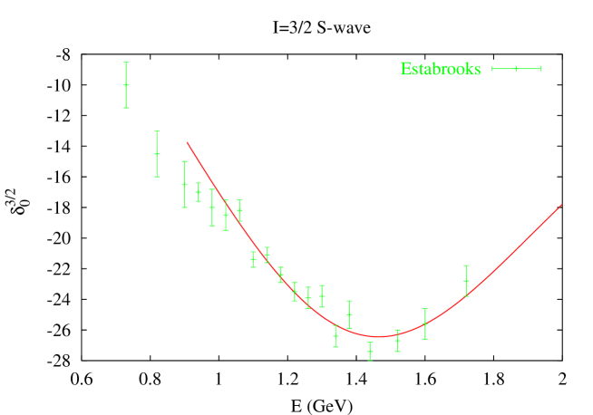
Figure 2: Experimental data from ref. [27] for the $I={3\over 2}$ $S$-wave phase shift

4.1 $\pi K\to\pi K$ data

Phase shift analyses of the $\pi K\to\pi K$ amplitude have been performed based on high-statistics production experiments $KN\to K\pi N$ by Estabrooks et al. [26] and by Aston et al. [27]. Earlier results are much less precise and we will not use them in our analysis. The amplitude $\pi^{+}K^{+}\to\pi^{+}K^{+}$ which is purely $I={3\over 2}$ has been measured by Estabrooks et al. [26]. In practice the $I={3\over 2}$ phase shifts are very small in the range $E\mathrel{\raise 2.58334pt\hbox{$<$}\kern-7.7778pt\lower 2.79857pt\hbox{$\sim$}}2$ GeV except for the $S$-wave. This phase shift is shown in fig.2 together with our fit, where a simple parametrization with three parameters is used

$$\tan\left(\delta_{0}^{3/2}(s)\right)={\alpha q\over 1+\beta q^{2}+\gamma q^{4}}$$ (58)

This parametrization is analogous to the one used in ref [19]. Inelasticity is neglected in this channel.

The amplitude $\pi^{+}K^{-}\to\pi^{+}K^{-}$ which involves the following isospin combination

$$F^{c}\equiv F^{1/2}+{1\over 2}F^{3/2}\ ,$$ (59)

was measured both in ref. [26] and ref. [27] – the latter experiment has better statistics and covers a larger energy range. The amplitude $F^{c}$ can be expanded over partial-waves in the same way as eq. (4) and refs. [26, 27] provide the phase $\Phi_{l}(s)$ and the modulus $a_{l}(s)$ of these partial waves,

$$f^{c}_{l}(s)\equiv\sqrt{2l+1}\,a_{l}(s){\rm e}^{i\Phi_{l}(s)}\ .$$ (60)

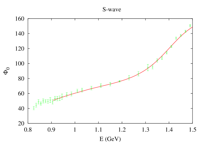
Figure 3: Experimental data from ref. [27] for the phase $\Phi_{0}$ and the fit used in the calculations.

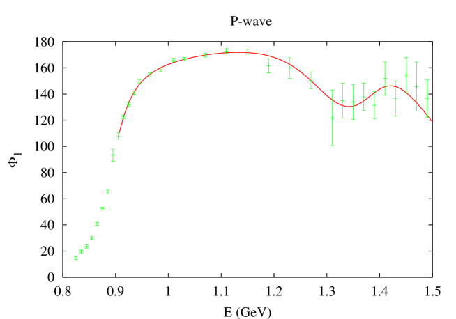
Figure 4: Experimental data from ref. [27] for the phase $\Phi_{1}$ and the fit used in the calculations.

Performing a combined fit of the $I={3\over 2}$ partial waves [26] and of the parameters $a_{l}$, $\Phi_{l}$ [26, 27] one can separate the two isospin partial waves. The data of Aston et al. for the phases $\Phi_{0}$ and $\Phi_{1}$ and our fits are displayed in figs. 3 and 4 respectively in the range $0.9\leq E\leq 1.5$ GeV (this energy region plays an important role in our analysis). The fits shown here correspond to a parametrization of the partial-wave $S$-matrices as products of Breit-Wigner $S$-matrices, allowing for inelasticity in the $I={1\over 2}$ amplitude to set in at the $\eta K$ threshold. Inelasticity is found to remain quite small up to $E\simeq 1.5$ GeV. We also tried different fits based on K-matrix parametrizations.

The data of Aston et al. and the fits for both $a_{l}$ and $\Phi_{l}$ for $l=0$ to $l=5$ and energy up to $E=2.5$ GeV are shown in figs. 5, 6 and 7. At energies $E\geq 1.8$ GeV, ref. [27] found two different solutions A and B for the phase shifts, between which we choose sol A (it was pointed out in ref. [19] that solution B violates the unitarity bound). These fits allow us to compute the relevant integrals up to $E=2.5$ GeV. Above that point, we use a Regge-model parametrization discussed in sec. 4.3.

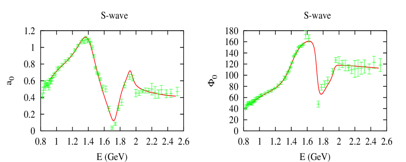
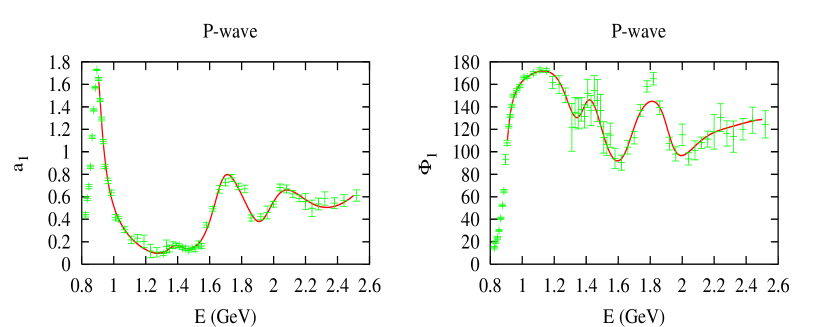
Figure 5: Modulus and phase of the $S$- and $P$-partial-waves amplitudes from ref. [27] and the fits in the region $0.9\leq E\leq 2.5$ GeV which are used in the calculations.

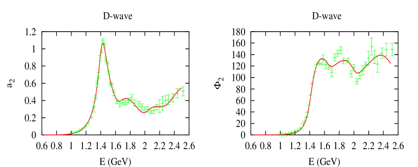
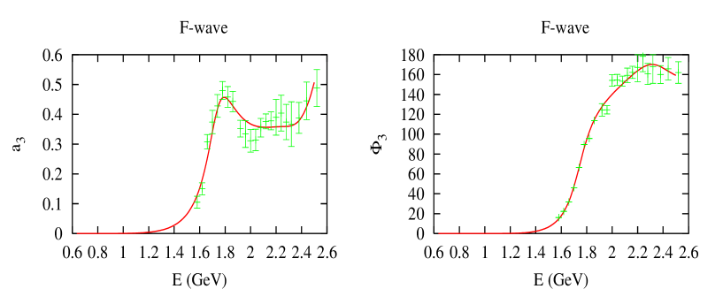
Figure 6: Same as fig.5 for the $D$- and $F$-partial waves.

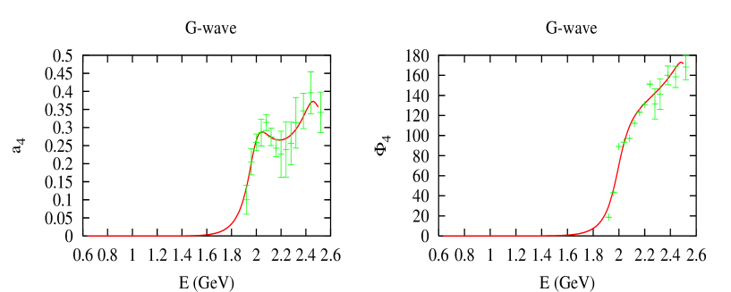
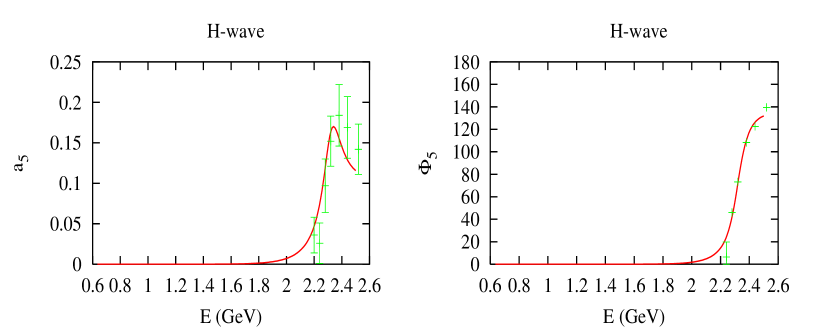
Figure 7: Same as fig.5 for the $G$- and $H$-partial waves.

4.2 $\pi\pi\to K\overline{K}$ input

For our purposes, a key role is played by the $l=0$ and $l=1$ $\pi\pi\to K\overline{K}$ amplitudes, which can be determined from $\pi N\to K\overline{K}N$ production experiments in the range $t\geq 4m^{2}_{K}$. We will make use of the two high-statistics experiments described in Cohen et al. [28] and Etkin et al. [29, 47]. The experiment of Cohen et al. [28] determines the charged amplitude $\pi^{+}\pi^{-}\to K^{+}K^{-}$, thereby providing results for both $g_{0}^{0}$ and $g_{1}^{1}$. There are several possible solutions but physical requirements select a single one, called solution II b in ref. [28]. Close to the $K\overline{K}$ threshold, the presence of the $l=1$ phase allows the authors to accurately determine the $l=0$ phase. The experiment of Etkin et al. concerns the amplitude $\pi^{+}\pi^{-}\to K_{S}K_{S}$ which is purely $I=0$. Because of the absence of the $P$-wave in this channel, their determination of the phase of $g_{0}^{0}$ close to the threshold (where the $D$-wave phase is very small) is likely to be less reliable than that of ref. [28]. Their determination of the magnitude of $g_{0}^{0}$ close to the threshold disagrees with that of Cohen et al. and also with earlier experiments [48]. Consequently, we make the choice to use the results of Etkin et al. only in the range $\sqrt{t}\geq 1.2$ GeV.

Our input for the phase of $g_{0}^{0}$ is determined as follows. Below the $K\overline{K}$ threshold this phase is identical to the $\pi\pi$ phase shift because of the elastic unitarity assumption. In the range $2m_{\pi}\leq E\leq 0.8$ GeV we use solutions of the $\pi\pi$ Roy equations. Simple parametrizations were provided recently in refs. [6, 11]. We use the parametrization of ref. [11] together with the scattering lengths corresponding to the “extended” fit, with the central values $a_{0}^{0}=0.228$, $a_{0}^{2}=-0.0382$. In the range $E\geq 2m_{K}$ we perform piecewise-polynomial fits of the data of refs. [28, 29] and fixing the threshold value to $\Phi_{0}^{0}=200\pm 15$ degrees. This range is an educated guess based on considering the data of Cohen et al. as well as $\pi\pi$ data. Finally in the range $0.8\textrm{ GeV}\leq E\leq 2m_{K}$ we perform a fit to the CERN-Munich data as given by Hyams et al. [49] and to the polarized target production data recently analyzed by Kaminski et al. [50]. For the modulus of $g_{0}^{0}$, we have performed piecewise polynomial fits to the data of refs. [28, 29]. The data and these fits are shown in fig.8.

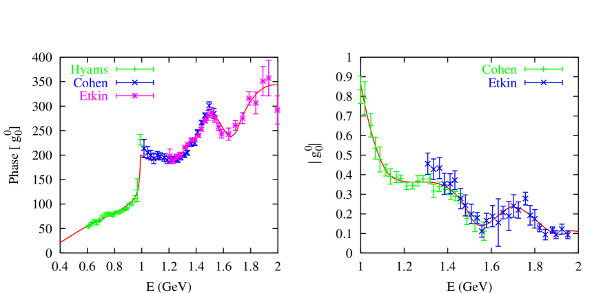
Figure 8: Inputs for the phase of $g_{0}^{0}$ above the $\pi\pi$ threshold and its modulus above the $K\overline{K}$ threshold. The data are from refs. [49, 28, 29].

As far as $g_{1}^{1}$ is concerned, we use the experimental determination of the $\pi\pi$ $P$-wave phase in the range $2m_{\pi}\leq E\leq 2m_{K}$ obtained from the pion vector form factor measured by CLEO [51]. This determination is compatible with the results of the analysis of $\pi\pi$ Roy equations and has a comparable accuracy. At larger energies, we use the experimental results from Cohen et al. for the phase and the magnitude of $g_{1}^{1}$. The whole energy range where data are available can be fitted using the following form

$$g_{1}^{1}(t)={C\over(1+r_{1}q^{2}_{\pi}(t))^{1\over 2}(1+r_{1}q^{2}_{K}(t))^{1\over 2}}\times$$

$$\phantom{g_{1}^{1}(t)={C}}\left\{BW(t,m_{\rho})+(\beta+\beta_{1}q^{2}_{K}(t))BW(t,m_{\rho^{\prime}})+(\gamma+\gamma_{1}q^{2}_{K}(t))BW(t,m_{\rho^{\prime\prime}})\right\}$$ (61)

with

$$BW^{-1}(t,m_{V})=m^{2}_{V}-t-i\sqrt{t}\>\Gamma_{V}{2G_{\pi}(t)+G_{K}(t)\over 2G_{\pi}(m^{2}_{V})},\ G_{P}(t)=\sqrt{t}\left({2q_{P}(t)\over\sqrt{t}}\right)^{3}\ .$$ (62)

Below the $K\overline{K}$ threshold, $q^{2}_{K}(t)$ vanishes and expression (4.2) reduces to the Kühn and Santamaria [52] form used in ref. [51]. We take the values of the parameters $\beta$, $\gamma$, $m_{\rho}$, $m_{\rho^{\prime}}$, $m_{\rho^{\prime\prime}}$ determined by CLEO and we fit the parameters $C$, $r_{1}$, $\beta_{1}$, $\gamma_{1}$ to the data above the $K\overline{K}$ threshold. The data and the fits are shown in fig. 9.

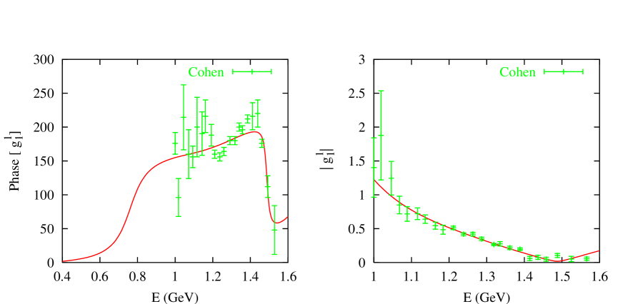
Figure 9: Input for the phase and the magnitude of $g_{1}^{1}$. The data shown are from ref. [28] and the curve is the fit from eq. (4.2).

The amplitudes with $l\geq 2$ play a much less significant role in our analysis and are suppressed at low energies. They will be described by simple Breit-Wigner parametrizations associated with the resonances $f_{2}(1200)$, $f^{\prime}_{2}(1525)$, $\rho_{3}(1690)$, $f_{4}(2050)$. Masses and partial decay widths of these resonances were taken from the PDG [53].

4.3 Asymptotic regions

As discussed above, we can make use of the partial-wave expansion and experimental data up to energies $E=\sqrt{s_{2}}=2.5$ GeV for the $s$- as well as the $t$-channel. Above that point we use a description of the amplitudes based on Regge phenomenology. We will content ourselves with very unsophisticated models because this energy region turns out to play a very minor role in our analysis. In the regime $s^{\prime}\to\infty$, $t$ fixed, we use the following expression for the amplitudes suggested by dual models à la Veneziano [54, 55, 56, 57] (where exact exchange degeneracy is built in)

$${\rm Im}\,F^{-}(s^{\prime},t)|_{\rm asy}\sim{\pi\lambda\over\Gamma({\alpha^{\rho}}+\alpha_{1}t)}(\alpha_{1}s^{\prime})^{{\alpha^{\rho}}+\alpha_{1}t}$$ (63)

and

$${\rm Im}\,F^{+}(s^{\prime},t)|_{\rm asy}\sim\sigma s^{\prime}{\exp}\left({bt\over 2}\right)+{\rm Im}\,F^{-}(s^{\prime},t)|_{\rm asy}\ .$$ (64)

For the parameter $\lambda$ and the Pomeron parameters $\sigma$, $b$ we adopt values inspired by the discussion in App. B.4 of ref. [6] with large errors

$$\lambda=14\pm 5\ ,\ \sigma=5\pm 2.5{\ \rm mb}\ ,\ b=8\pm 3\ {\rm GeV}^{-2}\ .$$ (65)

The intercept and slope parameters of the Regge trajectories are determined from the experimental spectrum of the $\rho$ and $K^{*}$ resonances,

$${\alpha^{K^{*}}}=0.352,\quad{\alpha^{\rho}}=0.475,\quad\alpha_{1}=0.882\ {\rm GeV^{-1}}\ .$$ (66)

For illustration we compare in fig. 10 the imaginary part of $F^{-}(s,0)$ resulting from our fit to the experimental data and the Regge asymptotic form with $\lambda=14$ .

Making use of this, it is easy to evaluate the contributions to the various dispersive integrals in the range $[s_{2},\infty]$. In the fixed-$t$ DR’s we obtain

$$F^{+}(s,t)|_{s_{2}}={2(\lambda_{s}+st)\over(s_{2})^{2}}\left[{\sigma s_{2}\over\pi}{\rm exp}{bt\over 2}+{\lambda\over(2-{\alpha^{\rho}}-\alpha_{1}t)\Gamma({\alpha^{\rho}}+\alpha_{1}t)}(\alpha_{1}s_{2})^{{\alpha^{\rho}}+\alpha_{1}t}\right]$$

$$\phantom{F^{+}(s,t)_{s_{2}}}+{t^{2}\over(s_{2})^{2}}\left[{\lambda\over(2-{\alpha^{K^{*}}})\Gamma({\alpha^{K^{*}}})}(\alpha_{1}s_{2})^{\alpha^{K^{*}}}\right]$$ (67)

and

$$F^{-}(s,t)|_{s_{2}}={s-u\over(s_{2})^{2}}\left[t\,{\lambda(\alpha_{1}s_{2})^{\alpha^{K^{*}}}\over(2-{\alpha^{K^{*}}})\Gamma({\alpha^{K^{*}}})}+{\lambda_{s}+st\over s_{2}}{\lambda(\alpha_{1}s_{2})^{{\alpha^{\rho}}+\alpha_{1}t}\over(3-{\alpha^{\rho}}-\alpha_{1}t)\Gamma({\alpha^{\rho}}+\alpha_{1}t)}\right]$$ (68)

In the same manner we can obtain the asymptotic contributions in the amplitudes described through hyperbolic DR’s

$${F^{-}(s_{b},t)\over s_{b}-u_{b}}\Bigg{|}_{s_{2}}={\Delta^{2}-b\over(s_{2})^{3}}{\lambda(\alpha_{1}s_{2})^{\alpha^{\rho}}\over(3-{\alpha^{\rho}})\Gamma({\alpha^{\rho}})}+{t\over(s_{2})^{2}}{\lambda(\alpha_{1}s_{2})^{\alpha^{K^{*}}}\over\Gamma({\alpha^{K^{*}}})}\Bigg{[}{1\over 2-{\alpha^{K^{*}}}}$$

$$\phantom{{F^{-}(s_{b},t)\over s_{b}-u_{b}}}-{\,b\,\alpha_{1}\over s_{2}(3-{\alpha^{K^{*}}})}\left(\log(\alpha_{1}s_{2})-\psi({\alpha^{K^{*}}})+{1\over 3-{\alpha^{K^{*}}}}\right)\Bigg{]}$$ (69)

and

$$F^{+}(s_{b},t)|_{s_{2}}={2(\Delta^{2}-b)\over(s_{2})^{2}}\left[{\sigma s_{2}\over\pi}+{\lambda(\alpha_{1}s_{2})^{\alpha^{\rho}}\over(2-{\alpha^{\rho}})\Gamma({\alpha^{\rho}})}\right]+{t(t-2\Sigma)\over(s_{2})^{2}}{\lambda(\alpha_{1}s_{2})^{\alpha^{K^{*}}}\over\Gamma({\alpha^{K^{*}}})}\Bigg{[}{1\over 2-{\alpha^{K^{*}}}}$$

$$\phantom{{F^{-}(s_{b},t)\over s_{b}-u_{b}}}-{\,b\,\alpha_{1}\over s_{2}(3-{\alpha^{K^{*}}})}\left(\log(\alpha_{1}s_{2})-\psi({\alpha^{K^{*}}})+{1\over 3-{\alpha^{K^{*}}}}\right)\Bigg{]}$$ (70)

To derive these contributions, we have used the following expression for ${\rm Im}\,G^{I}(t^{\prime},s^{\prime}_{b})$ in the regime where $t^{\prime}\to\infty$

$${1\over\sqrt{6}}{\rm Im}\,G^{0}(t^{\prime},s^{\prime}_{b})|_{asy}={1\over 2}{\rm Im}\,G^{1}(t^{\prime},s^{\prime}_{b})|_{asy}={\pi\lambda\over\Gamma({\alpha^{K^{*}}})}(\alpha_{1}t^{\prime})^{{\alpha^{K^{*}}}}\left\{1+{\alpha_{1}b\over t^{\prime}}(-\log(\alpha_{1}t^{\prime})+\psi({\alpha^{K^{*}}}))\right\}$$ (71)

in which an expansion to first order in the parameter $b$ has been performed.

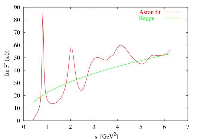
Figure 10: Comparison of ${\rm Im}\,F^{-}(s,0)$ constructed from experimental data and the Regge asymptotic form eq. (63).

5 Initial steps in the resolution

5.1 Solving for $g_{0}^{0}$, $g_{1}^{1}$

We have now all the ingredients to solve the set of RS equations. The first step consists in solving eqs. (2.5) for $g_{0}^{0}$, $g_{1}^{1}$. This problem was discussed a long time ago [58, 59] and we recall the main ideas here for completeness. Elastic unitarity implies that the phases $\Phi^{I}_{l}$ of these amplitudes

$$g^{I}_{l}(t)\equiv{\rm e}^{i\Phi^{I}_{l}(t)}|g^{I}_{l}(t)|$$ (72)

can be identified with the $\pi\pi$ phase shifts $\delta^{I}_{l}$ in the unphysical region $t<4m^{2}_{K}$ according to Watson’s theorem [60], and therefore they are known in principle. In the physical region $t\geq 4m^{2}_{K}$ the phases are determined from experiment as was discussed above.

On the other hand, the modulus of the $t$-channel partial waves is not known below the $K\bar{K}$ threshold, and must be determined using the equations (2.5) satisfied by $g_{0}^{0}$ and $g_{1}^{1}$ which have the following simple form

$$g_{0}^{0}(t)=\Delta_{0}^{0}(t)+{t\over\pi}\int_{4m^{2}_{\pi}}^{\infty}{dt^{\prime}\over t^{\prime}}{{\rm Im}\,g_{0}^{0}(t^{\prime})\over t^{\prime}-t},$$ (73)

$$g_{1}^{1}(t)=\Delta_{1}^{1}(t)+{t\over\pi}\int_{4m^{2}_{\pi}}^{\infty}{dt^{\prime}\over t^{\prime}}{{\rm Im}\,g_{1}^{1}(t^{\prime})\over t^{\prime}-t}\ .$$

In sec. 3, we have shown that these relations can be used up to $t\simeq 1.4\ {\rm GeV}^{2}$, which includes the whole region inaccessible to experiment where $|g_{0}^{0}|$, $|g_{1}^{1}|$ are needed. The quantities $\Delta^{I}_{l}(t)$ are analytic functions with a left-hand cut along the negative $t$ axis and no right-hand cut, as can be easily verified using eqs. (2.5) and the explicit form of the kernels provided in sec. 2. Therefore, determining the moduli $|g_{l}^{I}(t)|$ in the range $4m^{2}_{\pi}\leq t\leq{t_{m}}$ from eqs. (73) while the phase is known is a standard Muskhelishvili-Omnès problem [61, 62]. The most general solution involves arbitrary parameters, the number of which depend on the value of the phase at the matching point [61]. We have chosen ${t_{m}}$ to be slightly larger than $4m^{2}_{K}$. The $l=1$ phase $\Phi_{1}^{1}({t_{m}})$ is lower than $\pi$, which implies that the solution for $g_{1}^{1}$ involves no free parameter. The $l=0$ phase, as we argued in the previous section, satisfies $\pi\leq\Phi_{0}^{0}({t_{m}})<2\pi$, such that one free parameter is involved in the solution. Let us recall the explicit form of the solutions. One first introduces the Omnès function

$$\Omega^{I}_{l}(t)=\exp\left({t\over\pi}\int_{4m^{2}_{\pi}}^{{t_{m}}}{\Phi^{I}_{l}(t^{\prime})\,dt^{\prime}\over t^{\prime}(t^{\prime}-t)}\right)\equiv{\Omega^{I}_{l}}_{R}(t)\exp[i\Phi^{I}_{l}(t)\theta(t-4m^{2}_{\pi})\theta({t_{m}}-t)]$$ (74)

where ${\Omega^{I}_{l}}_{R}(t)$ is real. Then, the solutions of eqs. (73) read

$$g_{0}^{0}(t)=\Delta_{0}^{0}(t)+{t\Omega_{0}^{0}(t)\over{t_{m}}-t}\Bigg{[}\alpha_{0}+{t\over\pi}\int_{4m^{2}_{\pi}}^{{t_{m}}}dt^{\prime}\,{({t_{m}}-t^{\prime})\Delta_{0}^{0}(t^{\prime})\sin\Phi_{0}^{0}(t^{\prime})\over{\Omega^{0}_{0}}_{R}(t^{\prime})(t^{\prime})^{2}(t^{\prime}-t)}$$

$$\phantom{\Delta_{0}^{0}(t)+{t\Omega_{0}^{0}(t)\over{t_{m}}-t}\Bigg{[}\alpha_{0}}+{t\over\pi}\int_{t_{m}}^{\infty}dt^{\prime}\,{({t_{m}}-t^{\prime})|g_{0}^{0}(t^{\prime})|\sin\Phi_{0}^{0}(t^{\prime})\over{\Omega^{0}_{0}}_{R}(t^{\prime})(t^{\prime})^{2}(t^{\prime}-t)}\Bigg{]}$$ (75)

$$g_{1}^{1}(t)=\Delta_{1}^{1}(t)+t\Omega_{1}^{1}(t)\Bigg{[}{1\over\pi}\int_{4m^{2}_{\pi}}^{{t_{m}}}dt^{\prime}\,{\Delta_{1}^{1}(t^{\prime})\sin\Phi_{1}^{1}(t^{\prime})\over{\Omega^{1}_{1}}_{R}(t^{\prime})t^{\prime}(t^{\prime}-t)}$$

$$\phantom{\Delta_{0}^{0}(t)+{t\Omega_{0}^{0}(t)\over{t_{m}}-t}\Bigg{[}\alpha_{0}}+{1\over\pi}\int_{t_{m}}^{\infty}dt^{\prime}\,{|g_{1}^{1}(t^{\prime})|\sin\Phi_{1}^{1}(t^{\prime})\over{\Omega^{1}_{1}}_{R}(t^{\prime})t^{\prime}(t^{\prime}-t)}\Bigg{]}$$ (76)

Notice that the integrands are singular when $t^{\prime}\to t_{m}$, since the Omnès function behaves as

$${\Omega^{I}_{l}}_{R}(t^{\prime})\sim|t^{\prime}-t_{m}|^{\phi_{l}^{I}(t_{m})\over\pi}$$ (77)

but the singularity is integrable. When $t\to t_{m}$ the integrands diverge but this is compensated by the factor of $\Omega_{l}^{I}(t)$ multiplying the integrals. It can be shown that the solution satisfies automatically the first matching condition (details of the proof are given in App. A)

$$\lim_{\epsilon\to 0}g_{l}^{I}(t_{m}\pm\epsilon)|_{\rm sol}=g_{l}^{I}(t_{m})|_{\rm input}\ .$$ (78)

Here, $g_{0}^{0}(t)$, $g_{1}^{1}(t)$ are treated in a somewhat different way from that in ref. [15]. In that work, an additional subtraction constant was introduced and the values of the subtraction parameters were fixed by imposing that the values of $g^{1}_{1}(0)$, $g^{0}_{0}(0)$ and ${d\over dt}g^{0}_{0}(0)$ be equal to the ChPT prediction at order $p^{2}$. Now, the behaviour around $t=0$ is entirely determined by solving the full set of equations with the appropriate boundary conditions – our constraints are dispersive and do not rely on ChPT results.

At this stage, the formulas (5.1),(5.1) for $g_{0}^{0}(t)$, $g_{1}^{1}(t)$ involve three parameters: the two $S$-wave scattering lengths $a_{0}^{1/2}$, $a_{0}^{3/2}$ that appear in the expressions for $\Delta_{0}^{0}(t)$, $\Delta_{1}^{1}(t)$ and an additional parameter $\alpha_{0}$. We will now clarify their role.

5.2 Matching conditions and uniqueness

Once $g_{0}^{0}(t)$, $g_{1}^{1}(t)$ are expressed according to eqs. (5.1),(5.1), the set of four RS equations (2.4) becomes a closed set of equations for the four $\pi K$ partial waves $f^{I}_{l}(s)$, $l=0,1$, $I={1\over 2},\ {3\over 2}$ . The structure of these equations is similar to that of $\pi\pi$ Roy equations: the kernels consist of a singular Cauchy part and a regular part, and elastic unitarity provides a non-linear relation between ${\rm Re}\,f^{I}_{l}(s)$ and ${\rm Im}\,f^{I}_{l}(s)$. The equations must be solved with the boundary condition that the solution phase shifts must equate the input phase shifts at the frontier of the region of resolution (matching condition). Therefore, we can apply the results derived recently [34, 35] concerning the number of independent solutions in the vicinity of a given solution. The multiplicity index of one solution is determined by the values of the input phase shifts at the matching point $s=s_{m}$ (with $s_{m}\simeq 0.935$ GeV²). The experimental phase shifts at $s=s_{m}$ lie in the following ranges

$$0<\delta_{0}^{1/2}(s_{m})<{\pi\over 2},\ \ {\pi\over 2}<\delta_{1}^{1/2}(s_{m})<{\pi},\ \ \delta_{0}^{3/2}(s_{m})<0,\ \ \delta_{1}^{3/2}(s_{m})<0.$$ (79)

According to the discussion in ref. [35], the multiplicity index in this situation is $m=0+1-1-1=-1$, to be compared with $m=0$ in the case of $\pi\pi$. This means that our situation corresponds to a constrained system: a solution will not exist unless the two $S$-wave scattering lengths lie on a one dimensional curve.

In practice, however, the phase shift for the $I={3\over 2}$, $P$-wave is extremely small below 1 GeV and the experimental input is not precise enough to implement matching conditions in this channel in any meaningful way (see fig. 17 below). This leads us to treat the $I={3\over 2}$ P-wave on the same footing as the partial waves with $l\geq 2$. For instance, the dispersive representations can be projected on $l=2$ and used to compute the real part of $f^{1/2}_{2}(s)$ for $s\leq s_{m}$ while the contribution of ${\rm Im}\,f^{1/2}_{2}(s^{\prime})$ for $s^{\prime}\leq s_{m}$ in the integrands is negligibly small compared to contributions from $S$- and $P$-waves; it can be evaluated approximately or even ignored . Dropping one matching condition, the effective multiplicity index becomes $m=0$ for $\pi K$. The fact that the multiplicity index vanishes means that solutions should exist for arbitrary values of the two $S$-wave scattering lengths $a_{0}^{1/2}$, $a_{0}^{3/2}$ lying in some two dimensional region, and each solution is unique.

However, not all solutions are physically acceptable. An acceptable solution must satisfy the further requirement that it displays no cusp at the matching point [6]. This condition leads to constraints on the subtraction parameters. First, let us consider the $t$-channel, for which we choose the matching point $t_{m}$ to be slightly larger than the $K\overline{K}$ threshold. As discussed in the previous section, the solution for $g_{0}^{0}(t)$ involves one parameter $\alpha_{0}$. While the equality $g_{0}^{0}|_{\rm sol}=g_{0}^{0}|_{\rm input}$ is automatically guaranteed by eq. (5.1), the solution $g_{0}^{0}|_{\rm sol}$ exhibits a sharp cusp at the matching point in general. Therefore, the no-cusp condition fixes the value of $\alpha_{0}$. The same reasoning can be applied to the $\pi K$ partial waves: imposing the no-cusp condition to the $I={1\over 2}$ $S$- and $P$-waves provides two equations which should determine, in principle, the two scattering lengths $a_{0}^{1/2}$, $a_{0}^{3/2}$. In other words, given ideal experimental input data with no errors in the ranges $s\geq s_{m}$ and $t\geq t_{m}$, one should be able to fix exactly the two scattering lengths by solving the RS equations with the appropriate boundary conditions on the values and the derivatives of the phase shifts. Obviously, the actual situation is different from that ideal view: the input data are known with errors and only for discrete values of the energy, which introduces uncertainties on the boundary conditions and thus on the solutions of the RS equations. This point will be addressed in the following section.

6 Numerical solutions and results

6.1 Numerical determination of the solutions

We have described how to solve the RS equations for the $\pi\pi\to K\bar{K}$ partial waves. Assuming that the input for $s>s_{m}$ is given as well as the input for $l\geq 2$ at all energies, our purpose is to determine the three phase shifts

$$\delta^{0}(s)\equiv\delta_{0}^{1/2}(s),\quad\delta^{1}(s)\equiv\delta_{1}^{1/2}(s)\quad\delta^{2}(s)\equiv\delta_{0}^{3/2}(s)$$ (80)

in the range ${m^{2}_{+}}\leq s\leq s_{m}$, so that the Roy-Steiner equations represented symbolically as

$${\rm Re}\,f^{a}(s)\equiv{s\over\lambda_{s}}\sin(2\delta^{a}(s))=\Phi^{a}[\delta^{b},s]$$ (81)

are satisfied up to a certain accuracy. We introduce a set of $N$ mesh points ${m^{2}_{+}}<s_{i}\leq s_{m}$ ($N$ was varied between 16 and 30, the results were very stable) and characterize the accuracy of an approximate solution by the measure

$$\epsilon=\max_{i,a}|{\rm Re}\,f^{a}(s_{i})-\Phi^{a}[\delta^{b},s_{i}]|\ .$$ (82)

An exact solution, of course, satisfies $\epsilon=0$. While it is possible to search directly for minimums of $\epsilon$, a more appropriate quantity for minimization algorithms is the chi-square

$$\chi^{2}=\sum_{i=1}^{N}\sum_{a=0}^{2}|{\rm Re}\,f^{a}(s_{i})-\Phi^{a}[\delta^{b},s_{i}]\,|^{2}\ ,$$ (83)

which we have minimized using the MINUIT package [63]. Approximations to the $\pi K$ phase shifts $\delta^{a}(s)$ are constructed in the form of polynomials or piecewise polynomial parametrizations (we tried several forms) similar to that proposed by Schenk [64]. This is essentially the same method as in ref. [6] for the $\pi\pi$ Roy equations. The parameters are constrained so that the phase shifts are continuous at the matching point and the no-cusp condition applies to $\delta^{0}(s)$ and $\delta^{1}(s)$. As discussed in sec. 5.2, these additional conditions fix the values of the two $S$-wave scattering lengths, which are therefore included as two additional parameters in the minimization of the chi-square.

Let us denote by $n^{(a)}$ the number of parameters in the representation of $\delta^{a}$. Taking $n^{(0)}=3$, $n^{(1)}=2$, $n^{(2)}=1$ we obtain an approximation to the equation with $\epsilon\simeq 5\cdot 10^{-3}$. Adding one more parameter with $n^{(2)}=2$ makes $\epsilon$ go down to $\epsilon\simeq 2\cdot 10^{-3}$ and with still one more parameter, $n^{(2)}=3$, one obtains $\epsilon\simeq 1\cdot 10^{-3}$. This provides good evidence that the approximations are converging to a true solution. Seeking a much higher accuracy would be difficult: all integrals must be evaluated with a numerical precision better than $\epsilon$, and the computation of the phase shifts involve up to three successive numerical integrations (see eqs. (2.4),(74),(5.1),(5.1)).

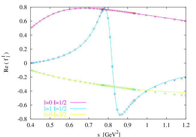
Figure 11: Left-hand sides of the RS equations. (2.4) (lines) compared to the right-hand sides (points) after minimization in the range ${m^{2}_{+}}\leq s\leq 0.93$ GeV² .

The accuracy of the solutions is illustrated in fig. 11. In particular, the figure shows that the left- and right-hand sides of the RS equations still agree with a good accuracy well above the matching point. This constitutes a consistency condition as discussed in ref. [6]. We have checked that its fulfilment is a direct consequence of imposing the no-cusp conditions. At this level, there is a notable difference between the $\pi\pi$ and the $\pi K$ RS equations. In the case of $\pi\pi$ scattering [6], it is found that imposing a single no-cusp condition for the $P$-wave is sufficient to ensure that the no-cusp condition holds to a good approximation for the $S$-waves as well, and the consistency conditions are well satisfied. In the $\pi K$ case, we find that it is necessary to impose no-cusp conditions for the two phase shifts $\delta_{0}^{1/2}(s)$ and $\delta_{1}^{1/2}(s)$. In fact, even after doing so, we find that a (small) cusp remains for the third phase shift $\delta_{0}^{3/2}(s)$. This does not represent a serious problem, in practice, because this phase shift is not determined very precisely in the vicinity of the matching point.

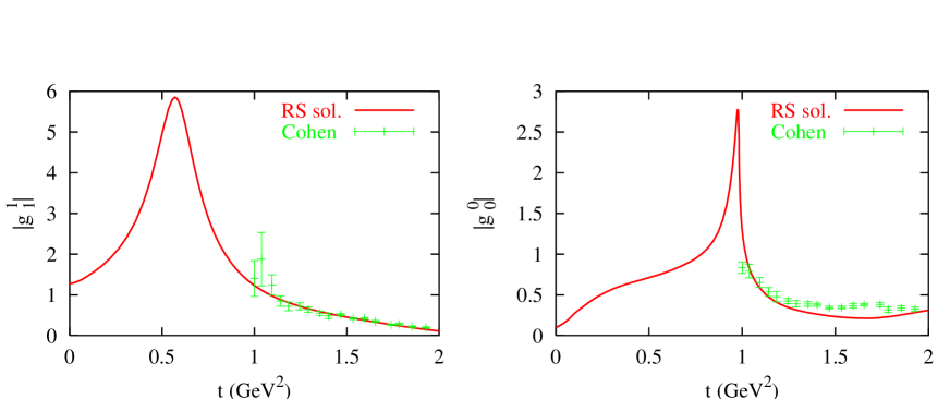
Figure 12: Comparison of the absolute values of $g_{0}^{0}$ and $g_{1}^{1}$ obtained from solving the RS equations and the corresponding experimental input from ref. [28].

Further consistency conditions ought to be considered in the $\pi\pi\to K\overline{K}$ sector. Here as well, one expects that the RS equations should be approximately satisfied above the matching point. This point is illustrated in fig.12 which compares the moduli of $g_{0}^{0}(t)$ and $g_{1}^{1}(t)$ computed from the RS equations to the experimental input for these quantities. Very good agreement is observed for $g_{1}^{1}(t)$. In contrast, we find that the agreement for $g_{0}^{0}(t)$ is moderately good. In the range $t\geq 4m^{2}_{K}$ we have checked that the unitarity bound $|S_{\pi\pi\to K\overline{K}}|\leq 1$ is obeyed. Adopting a larger value for the matching point $t_{m}$ improves the input-output agreement for $t>t_{m}$ but leads to violation of unitarity for $t<t_{m}$ close to the $K\overline{K}$ threshold.

Another consistency check can be performed. In the region where $t\leq 4m^{2}_{\pi}$, $g_{0}^{0}(t)$ and $g_{1}^{1}(t)$ can be obtained not only from eqs. (2.5) which are based on the fixed$-us$ dispersion relations but also from the fixed$-t$ ones which are valid in this domain. Both kinds of DR’s agree by construction at $t=0$, the fact that they should continue to agree for negative values of $t$ is not trivial and constitutes a check of consistency of the experimental input and of the RS solutions. We show these results for $t\leq 0$ in fig.13.

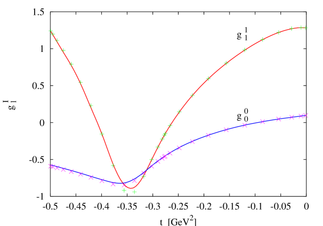
Figure 13: Plot of $g_{0}^{0}(t)$ and $g_{1}^{1}(t)$ in the region $t\leq 0$ obtained by projecting out two different kinds of dispersion relations. The lines are obtained from the fixed$-us$ DR’s and the points are obtained from the fixed$-t$ DR’s.

6.2 Error evaluations and the $S$-wave scattering lengths

Our general procedure for evaluating the errors consists in performing variations of the parameters which enter in the description of the input – making use of the errors on these parameters and their covariance matrices as provided by running the MINUIT package [63]. The experimental errors are assumed to be essentially of statistical origin and the errors at different energy points are assumed to be independent. Let us discuss first the case of the $I={1\over 2}$ $S$- and $P$-waves. It is clear that this part of the input plays a crucial role as it controls the boundary conditions which determine the two $S$-wave scattering lengths. To begin with, one notes that variations of the input in the energy region $E\mathrel{\raise 2.58334pt\hbox{$>$}\kern-7.7778pt\lower 2.79857pt\hbox{$\sim$}}1.5$ GeV has a negligibly small influence, so we will consider only the energy region $\sqrt{s_{m}}\leq E\leq 1.5$ GeV. We have performed two different kinds of fits in order to check the validity of the determination of the phase shifts, their derivatives, and the errors obtained from varying the parameters at the matching point $E=\sqrt{s_{m}}$. Firstly, we perform “global” fits based on a K-matrix parametrization with six parameters for the $S$-wave and seven parameters for the $P$-wave. These parameters are determined such as to minimize the chi-square in the energy region $0.90\leq E\leq 1.50$ GeV. Secondly, we have performed “local” fits in which one considers separately a small energy region surrounding the matching point $0.90\leq E\leq 1.1$ GeV and the remaining energy region. In the small region we approximate the $S$-wave phase shift by a quadratic polynomial,

$$\delta_{0}^{1/2}(s)=a+b(s-s_{m})+c(s-s_{m})^{2},\quad 0.90\leq E\leq 1.1\ {\rm GeV}$$ (84)

while for the $P$-wave we use a linear approximation after subtracting the tail of the $K^{*}$ resonance

$$\delta_{1}^{1/2}(s)-\arctan{m_{K^{*}}\Gamma_{K^{*}}\over m^{2}_{K^{*}}-s}=a+b(s-s_{m})\ .$$ (85)

The results from these two fits concerning the input at the matching point are shown in table 1. One observes that the determinations of the phases at the matching point are in good agreement as well as that of the errors. The determinations of the derivative of the $P$-wave agree while those of the derivative of the $S$-wave are only in marginal agreement. In this case, we consider the determination from the global fit to be somewhat more reliable as it has continuity and smoothness built in.

	phase	error	derivative	error
$l=0$ global	46.5	0.6	44.1	5.8
$l=0$ local	46.2	0.6	56.9	6.6
$l=1$ global	155.8	0.4	148.0	2.8
$l=1$ local	156.2	0.3	147.4	2.9

Table 1: $S$- and $P$-waves inputs at the matching point as determined from two different types of fit to the data of Aston et al. [27] (see text). Phases are in degrees and their derivatives in degrees$\times$GeV^-1.

We can now derive the constraints on the $S$-wave scattering lengths which arise upon solving the RS equations making use of the available experimental input above the matching point. Let us first quote some results concerning the errors. Table 2 shows how the errors affecting the various pieces of input propagate to the two $S$-wave scattering lengths. One can see that the two main sources of uncertainty are a) the $\pi K$ $I={1\over 2}$ $S$-wave and b) the $\pi\pi\to K\overline{K}$ $I=0$ $S$-wave. In contrast, the influence of the partial waves with $l\geq 2$ (in which the Regge region is also included) is rather modest. Finally, this analysis generates the following results for the scattering lengths $a^{I}_{0}$,

$$m_{\pi}\,a^{1/2}_{0}\simeq 0.224\pm 0.022,\quad m_{\pi}\,a^{3/2}_{0}\simeq(-0.448\pm 0.077)\>10^{-1}\ .$$ (86)

There is a significant correlation between these two quantities, the correlation parameter is positive and its value is

$$\rho_{{1\over 2}{3\over 2}}=0.908\ .$$ (87)

The one-sigma error ellipse corresponding to the above results for the $S$-wave scattering lengths is represented in fig.14. Our results are compatible with the band obtained for $a_{0}^{1/2},\ a_{0}^{3/2}$ in ref. [25]. We find a much smaller allowed region for the scattering lengths simply because we have used considerably better experimental input for the $S$- and $P$-waves: in the work of ref. [25] no data at all were available for $E\geq 1.1$ GeV. Predictions from ChPT at $O(p^{4})$ for the $S$-wave scattering lengths were presented in ref. [18]. They are recalled below

$$m_{\pi}a_{0}^{1/2}=0.19\pm 0.02\quad m_{\pi}a_{0}^{3/2}=-0.05\pm 0.02\qquad{\rm(ref.\ \cite[cite]{[\@@bibref{}{bkm2}{}{}]})}$$ (88)

	$f^{1/2}_{0}$	$f^{1/2}_{1}$	$f^{3/2}_{0}$	$g_{0}^{0}$	$g_{1}^{1}$	$l\geq 2$
$10^{2}\Delta{a^{1/2}_{0}}$	1.89	0.28	0.40	0.79	0.05	0.23
$10^{2}\Delta{a^{3/2}_{0}}$	0.55	0.09	0.39	0.32	0.14	0.11
$10^{2}\Delta(a^{1/2}_{0}-a^{3/2}_{0})$	1.35	0.18	0.10	0.55	0.10	0.15

Table 2: Sources of error arising from different parts of the input and the resulting errors in the determination of the $l=0$ scattering lengths in units of $m^{-1}_{\pi}$.

Within the errors these results appear compatible with those from the RS equations. A more refined comparison, however, should take the correlation into account. Computing the correlation parameter under the same assumptions as used in ref. [18] for the evaluation of the errors one obtains the standard error ellipse shown in fig. 14. One observes that the ChPT ellipse is very narrow and does not intersect the corresponding error ellipse resulting from the RS equations . If one judges from the size of the $O(p^{4})$ corrections as compared to the current algebra result, it seems not unreasonable to attribute the remaining discrepancy to $O(p^{6})$ effects. We quote also our results for the two combinations of scattering lengths proportional to $a_{0}^{-}$, $a_{0}^{+}$

$$m_{\pi}\,(a^{1/2}_{0}-a^{3/2}_{0})\simeq 0.269\pm 0.015,\quad m_{\pi}\,(a^{1/2}_{0}+2a^{3/2}_{0})\simeq 0.134\pm 0.037\$$ (89)

which are of interest in connection with the $\pi K$ atom: the square of the first combination is proportional to the inverse lifetime of the atom and the sum of the two combinations is proportional to the energy shift of the lowest atomic level [65]. The correlation parameter for $a_{0}^{-}$, $a_{0}^{+}$ is also positive and its value is

$$\rho_{-+}=0.925\ .$$ (90)

For comparison, let us mention the results for the combinations proportional to $a_{0}^{-}$, $a_{0}^{+}$ in ChPT,

$$m_{\pi}\,(a^{1/2}_{0}-a^{3/2}_{0})\simeq 0.238\pm 0.002,\quad m_{\pi}\,(a^{1/2}_{0}+2a^{3/2}_{0})\simeq 0.097\pm 0.047\quad\quad[{\rm ChPT\ {\it O}(p^{4})}]\ .$$ (91)

The uncertainty affecting $a_{0}^{-}$ is remarkably small. This, however, could be an artifact of the $O(p^{4})$ approximation. It remains to investigate how $O(p^{6})$ corrections affect this result.

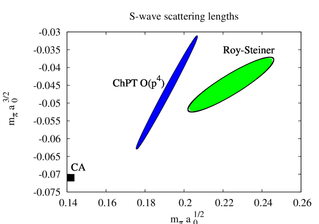
Figure 14: Standard error ellipse for the $S$-wave scattering lengths obtained from solving the RS equations with boundary conditions. The corresponding ellipse in the ChPT calculation at $O(p^{4})$ and the current-algebra result are also plotted.

As discussed above, the fact that the two $S$-wave scattering lengths are determined independently (to some extent) comes from imposing the no-cusp matching conditions. The difference of the two scattering lengths, $a^{1/2}_{0}-a^{3/2}_{0}$, can be determined in an alternative way from a sum rule [66] (see eq. (2.2)). Using this sum rule one finds

$$m_{\pi}(a^{1/2}_{0}-a^{3/2}_{0})=0.251\pm 0.014\quad\quad[{\rm sum\ rule}]\ .$$ (92)

In the evaluation, we use our results for the RS solutions in the integration regions $s^{\prime}\leq s_{m}$, $t^{\prime}\leq t_{m}$. The propagation of the experimental errors is studied in the same way as explained above. A rather small error is found, but one must keep in mind that the dependence on the asymptotic region is significant here and it is difficult to evaluate the error from this region in a very reliable way. The central value arising from the sum rule is smaller than what is obtained from the RS solution, but the two results are compatible within their errors. We also note that the output of the sum rule is significantly influenced by the values of the scattering lengths used as input in the integrand. For this reason, the result obtained here differs from the one quoted in ref. [15].

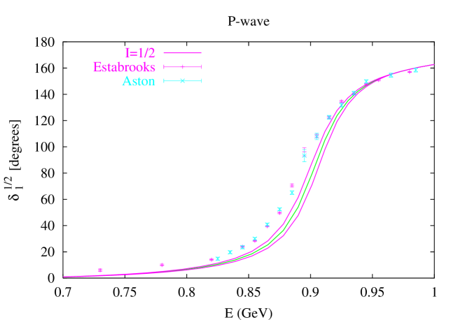
Figure 15: The $I={1\over 2}$ $P$-wave phase shift obtained from solving the RS equations. The central curve corresponds to solving with $a_{0}^{1/2},\ a_{0}^{3/2}$ taken at the center of the ellipse fig. 14. The upper (lower) curves are obtained by using the points with the maximal (minimal) values for $a_{0}^{1/2}$ on this ellipse.

Before we present the results for the amplitudes in the threshold region, a few remarks are in order concerning the intermediate energy region, that ranges from the threshold up to the matching point. Experimental data from production experiments exist below 1 GeV, but one has to keep in mind the possibility that systematic errors may have been underestimated in this energy region in such experiments (a discussion of the $\pi\pi$ case can be found in ref. [67]). Fig. 15 shows the $I={1\over 2}$ $P$-wave phase shift from the RS equations compared to experiment. The central curve correspond to solving with $a_{0}^{1/2},\ a_{0}^{3/2}$ taken at the center of the ellipse fig.14 while the upper and lower curves are obtained by using the points on the ellipse with the maximal and the minimal values for $a_{0}^{1/2}$ respectively. The experimental results are seen to deviate from the solutions as the energy decreases from the matching point. In particular, the mass of the $K^{*}$ which is predicted from the RS equations is

$$m_{K^{*}}=(905\pm 2)\ {\rm MeV}$$ (93)

(where $m_{K^{*}}$ is defined such that $\delta^{1/2}_{1}(m_{K^{*}})=\pi/2$) is nearly 10 MeV larger than the mass quoted in ref. [27] ($m_{K^{*0}}=896\pm 0.7$ MeV). This discrepancy may appear worrying at first sight. It is caused, in part, by isospin breaking which is not taken into account by the RS equations. This could generate an uncertainty of a few MeV as to the value of the $K^{*}$ mass that should come out from solving the equations. Besides, it cannot be excluded that the mass of the $K^{*}$ may not be as accurately known as one might believe. The determinations of the $K^{*+},\ K^{*0}$ masses used by the PDG are all based on hadronic production experiments. Recently, a measurement of the $K^{*+}$ mass based on the $\tau$ decay mode $\tau\to K_{S}\pi\nu_{\tau}$ indicated of shift by $4-5$ MeV as compared to the PDG value [68]. In principle, this method is more reliable because it is free of any final state interaction problem, but better statistics are needed to clarify this issue.

The two $S$-wave phase shifts predicted by the RS equations are shown in fig. 16. For the isospin $I={1\over 2}$ the RS solution does not exhibit any of the oscillations appearing in the data of ref. [26]. For the isospin $I={3\over 2}$ phase shift, the experimental data for $E<0.9$ GeV lie systematically below the RS curve, by 2-3 standard deviations. The RS equations also predict the $I={3\over 2}$ $P$-wave phase shift, the result is shown in fig.17. This phase shift displays the unusual feature that it is positive at very low energy and changes sign as the energy increases. In the region around 1 GeV the results are in qualitative agreement with the experimental data of Estabrooks et al.

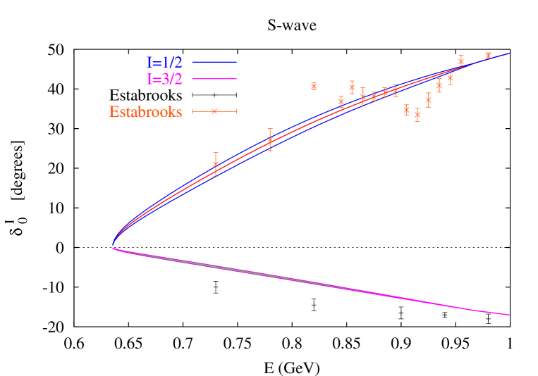
Figure 16: Same as fig. 15 for the $I={1\over 2}$ $S$-wave phase shift (curves in the upper half of the figure) and the $I={3\over 2}$ $S$-wave phase shift (curves in lower half).

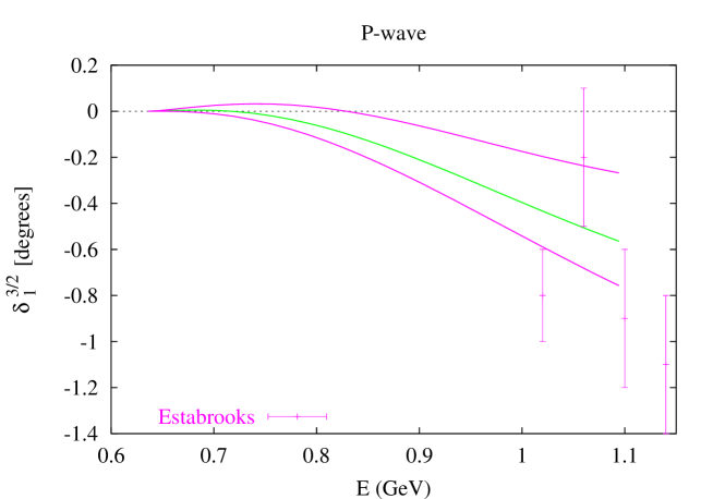
Figure 17: Same as fig. 15 for the $I={3\over 2}$ $P$-wave phase shift.

6.3 Results for threshold and sub-threshold expansion parameters

The behaviour of amplitudes at very small energies is conveniently characterized by sets of expansion parameters, which are particularly useful for making comparisons with chiral expansions. We consider first the set obtained by performing an expansion around the $\pi K$ threshold. These parameters are conventionally defined from the partial-wave amplitudes as follows

$${2\over\sqrt{s}}{\rm Re}f_{l}^{I}(s)=q^{2l}\left(a_{l}^{I}+b_{l}^{I}q^{2}+c_{l}^{I}q^{4}+\ldots\right)$$ (94)

with

$$s={m^{2}_{+}}+{{m^{2}_{+}}q^{2}\over m_{\pi}m_{K}}-{{m^{2}_{+}}{m^{2}_{-}}q^{4}\over 4m_{\pi}^{3}m_{K}^{3}}+\ldots$$ (95)

Once a solution of the RS equations is obtained, all the threshold parameters are predicted. The two $S$-wave scattering lengths are determined from the matching conditions, as explained above. The other threshold parameters may be obtained from the dispersive representation eq. (2.2) in the form of sum rules. These are obtained by projecting the DR’s over the relevant partial wave and then expanding the variable $s$ in powers of $q^{2}$. Divergences may appear in this process because derivatives are discontinuous at threshold and it must be specified that the limit is to be taken from above. This problem is easily handled by computing some pieces of the integrals analytically as explained in ref. [6]. The sum rules are evaluated by using RS solutions below the matching points and the fits to the experimental data above. For $l=0,\ 1$ we have computed the parameters $a_{l}$, $b_{l}$ and $c_{l}$ in an alternative manner by using our solution for ${\rm Re}\,f_{l}^{I}(s)$ for three values of $s$ and solving a linear system of equations. The two methods were in very good agreement and the results for the threshold parameters are summarized in table 3. The values of the $P$-waves scattering lengths in ChPT at NLO was given in ref.[18]

$$m^{3}_{\pi}a_{1}^{1/2}=0.016\pm 0.003\quad m^{3}_{\pi}a_{1}^{3/2}=(1.13\pm 0.57)\,10^{-3}\qquad{\rm(ref.\ \cite[cite]{[\@@bibref{}{bkm2}{}{}]})}\ .$$ (96)

Within the errors, these values are compatible with our corresponding results displayed in table 3.

	$I={1\over 2}$	$I={3\over 2}$	$\left(I={1\over 2}\right)-\left(I={3\over 2}\right)$
$m^{3}_{\pi}\>a_{1}^{I}$	$(0.19\pm 0.01)10^{-1}$	$(0.65\pm 0.44)10^{-3}$	$(0.18\pm 0.01)10^{-1}$
$m^{5}_{\pi}\>a_{2}^{I}$	$(0.47\pm 0.03)10^{-3}$	$(-0.11\pm 0.27)10^{-4}$	$(0.48\pm 0.01)10^{-3}$
$m^{7}_{\pi}\>a_{3}^{I}$	$(0.23\pm 0.03)10^{-4}$	$(0.91\pm 0.30)10^{-5}$	$(0.14\pm 0.01)10^{-4}$
$m^{3}_{\pi}\>b_{0}^{I}$	$(0.85\pm 0.04)10^{-1}$	$(-0.37\pm 0.03)10^{-1}$	$0.12\pm 0.01$
$m^{5}_{\pi}\>b_{1}^{I}$	$(0.18\pm 0.02)10^{-2}$	$(-0.92\pm 0.17)10^{-3}$	$(0.27\pm 0.01)10^{-2}$
$m^{7}_{\pi}\>b_{2}^{I}$	$(-0.14\pm 0.03)10^{-3}$	$(-0.96\pm 0.26)10^{-4}$	$(-0.48\pm 0.02)10^{-4}$
$m^{5}_{\pi}\>c_{0}^{I}$	$(-0.45\pm 0.04)10^{-1}$	$(0.18\pm 0.02)10^{-1}$	$(-0.62\pm 0.06)10^{-1}$
$m^{7}_{\pi}\>c_{1}^{I}$	$(0.71\pm 0.11)10^{-3}$	$(0.51\pm 0.09)10^{-3}$	$(0.20\pm 0.03)10^{-3}$

Table 3: Results for the threshold expansion parameters (see eq. (94) ) computed from the dispersive representations and the RS equations solutions. The third column shows the difference of the $I={1\over 2}$ and the $I={3\over 2}$ parameters

ChPT expansions of the amplitude are expected to have best convergence properties in unphysical regions away from any threshold singularity. The dispersive representations derived in sec. 2 allow us to evaluate the amplitude in such regions. A first domain considered in the literature is the neighbourhood of the point $s=u$, $t=0$. The following set of expansion parameters are conventionally introduced

$$F^{+}(s,t)=\sum\tilde{C}^{+}_{ij}\,t^{i}\nu^{2j}$$

$$F^{-}(s,t)=\nu\,\left\{\,\sum\tilde{C}^{-}_{ij}\,t^{i}\nu^{2j}\right\}$$ (97)

where

$$\nu={s-u\over 4m_{K}}\ .$$ (98)

It is customary to quote the values of the dimensionless parameters $C^{\pm}_{ij}$ which are related to $\tilde{C}^{\pm}_{ij}$ by

$$C^{+}_{ij}=(m_{\pi^{+}})^{2i+2j}\,\tilde{C}^{+}_{ij},\quad C^{-}_{ij}=(m_{\pi^{+}})^{2i+2j+1}\,\tilde{C}^{-}_{ij}\ .$$ (99)

The results for the subthreshold expansion parameters are collected in table 4. The table also shows for comparison results from ref. [69], which used fits to the experimental data of Estabrooks et al. [26] combined with earlier sets of data (taking into account the data points below 1 GeV as well as above). The authors of ref. [69] observed that the low-energy part of the data of Estabrooks et al leads to inconsistencies with a dispersive representation of $F^{-}$. The agreement with our results is reasonable for the coefficients $C^{-}_{ij}$. For the coefficients $C^{+}_{ij}$ the results are compatible within the errors, except for the coefficient $C^{+}_{10}$, for which we find a somewhat larger value. Another point of interest is the Cheng-Dashen point $s=u$, $t=2m^{2}_{\pi}$. The value of the amplitude $F^{+}$ at this point can be related to the kaon sigma-term [70] (see [71] for a recent review). We obtain for this quantity

$$F^{+}(m^{2}_{K},2m^{2}_{\pi})=3.90\pm 1.50\ .$$ (100)

				ref. [69]	$SU(3)$	$SU(2)$
		$C^{-}_{00}$	$8.92\pm 0.38$	$7.31\pm 0.90$	2	1
$C^{+}_{00}$	$2.01\pm 1.10$			$-0.52\pm 2.03$	2	2
$C^{+}_{10}$	$0.87\pm 0.08$			$0.55\pm 0.07$	2	2
$C^{+}_{01}$	$2.07\pm 0.10$			$2.06\pm 0.22$	4	2
		$C^{-}_{10}$	$0.31\pm 0.01$	$0.21\pm 0.04$	4	3
$C^{+}_{20}$	$(0.24\pm 0.06)10^{-1}$				4	4
		$C^{-}_{01}$	$0.62\pm 0.06$	$0.51\pm 0.10$	6	3
$C^{+}_{11}$	$(-0.66\pm 0.10)10^{-1}$			$-0.04\pm 0.02$	6	4
		$C^{-}_{20}$	$(0.85\pm 0.01)10^{-2}$		6	5
$C^{+}_{30}$	$(0.34\pm 0.08)10^{-2}$				6	6
$C^{+}_{02}$	$0.34\pm 0.03$				8	4

Table 4: Results for the dimensionless subthreshold expansion parameters defined in eqs. (6.3) and (99). The last two columns indicate the chiral order of the leading tree-level contribution to each parameter in $SU(3)$ and $SU(2)$ ChPT respectively.

6.4 Some implications for the $O(p^{4})$ chiral couplings

In this section we present some results on the $O(p^{4})$ couplings of the $SU(3)$ chiral expansion, which are easily derived from the subthreshold parameters obtained above. More detailed comparisons between chiral expansions and dispersive representations of the $\pi K$ scattering amplitude should be performed, but this is left for future work. The expression for this amplitude in ChPT at order $p^{4}$ was presented in ref. [17]. More specifically, we will make use of a reformulation of the expression of ref. [17] in which $F_{0}$ is expressed in terms of $F_{\pi}$ only (and not $F_{K}$) as in ref. [15] (a factor $\bar{J}_{\pi K}(s)$ is missing in eq. (41) of that reference). From this, it is straightforward to obtain the chiral formulas for the subthreshold expansion parameters. We present these in numerical form below, in which we use the following values for the masses, the pion decay constant and the renormalization scale $\mu$

$$m_{\pi}=0.13957,\ m_{K}=0.4957,\ m_{\eta}=0.5473,\ F_{\pi}=0.0924,\ \mu=0.77\ \rm{(all\ in\ GeV)}\ .$$ (101)

The dimensionless subthreshold parameters $C^{+}_{ij}$ then have the following numerical expressions in ChPT at NLO

$$C^{+}_{00}=0.14985+{8m^{2}_{\pi}m^{2}_{K}\over F^{4}_{\pi}}\left[4L_{1}+L_{3}-(4L_{4}+L_{5})+2(L_{8}+2L_{6})\right]$$

$$C^{+}_{10}=0.45754+{4(m^{2}_{K}+m^{2}_{\pi})m^{2}_{\pi}\over F^{4}_{\pi}}\left[-(4L_{1}+L_{3})+2L_{4}\right]+{2m^{4}_{\pi}\over F^{4}_{\pi}}L_{5}$$

$$C^{+}_{20}=0.02554+{2m^{4}_{\pi}\over F^{4}_{\pi}}\left[4L_{1}+L_{2}+{5\over 4}L_{3}\right]$$

$$C^{+}_{01}=1.67285+{8m^{2}_{K}m^{2}_{\pi}\over F^{4}_{\pi}}\left[4L_{2}+L_{3}\right]$$ (102)

while the subthreshold parameters $C^{-}_{ij}$ read

$$C^{-}_{00}=8.42568+{8m_{K}m^{3}_{\pi}\over F^{4}_{\pi}}L_{5}$$

$$C^{-}_{10}=-0.02533-{4m_{K}m^{3}_{\pi}\over F^{4}_{\pi}}L_{3}\ .$$ (103)

In order to lighten the notations we have denoted the renormalized couplings $L^{r}_{i}(\mu=0.77)$ simply by $L_{i}$. It is now easy to solve for the $L_{i}$’s making use of the results from table 4, the results for $L_{1},...,L_{4}$ are collected in table 5. The errors are obtained, as before, by varying all the parameters of the fits to the input data and taking into account the correlations. These errors appear to be rather small but they only reflect the uncertainty coming from the input data. The dominant source of uncertainty in the determination of the $L_{i}$’s comes from the unknown higher-order terms in the chiral expansion, this uncertainty is expected to be of the order of 30-40% . This can be seen from the table which shows the results of some alternative determinations based on the $Kl_{4}$ form factors [72, 73, 16] and on $\pi K$ sum rules [15]. We also quote the results that we get for $L_{5}$ and for $L_{8}+2L_{6}$ which have rather large errors

$$10^{3}L_{5}=3.19\pm 2.40\quad 10^{3}(L_{8}+2L_{6})=3.66\pm 1.52\ .$$ (104)

The coupling $L_{5}$ is determined, in principle, from $C^{-}_{00}$ but its contribution turns out to be suppressed, as it appears multiplied by a factor $m^{2}_{\pi}$. In order to determine $L_{8}+2L_{6}$ we used $C^{+}_{00}$ and the value $L_{5}\simeq 1.4\cdot 10^{-3}$ derived from $F_{K}/F_{\pi}$. The large uncertainty for $L_{8}+2L_{6}$ reflects that affecting the coefficient $C^{+}_{00}$ or, alternatively, the uncertainty in the combination of scattering lengths $a^{1/2}_{0}+2a^{3/2}_{0}$. This could improve considerably once experimental results from $\pi K$ atoms are available. Our result for $L_{4}$, though affected by a sizeable error, agrees with the evaluations [74, 75] based on a dispersive method for constructing scalar form factors [76] and is suggestive of a significant violation of the OZI rule in the scalar sector.

	$\pi K$ Roy-Steiner	$\pi K$ sum-rules	$Kl_{4},\ O(p^{4})$	$Kl_{4},\ O(p^{6})$
$10^{3}\,L_{1}$	$1.05\pm 0.12$	$0.84\pm 0.15$	$0.46\pm 0.24$	$0.53\pm 0.25$
$10^{3}\,L_{2}$	$1.32\pm 0.03$	$1.36\pm 0.13$	$1.49\pm 0.23$	$0.71\pm 0.27$
$10^{3}\,L_{3}$	$-4.53\pm 0.14$	$-3.65\pm 0.45$	$-3.18\pm 0.85$	$-2.72\pm 1.12$
$10^{3}\,L_{4}$	$0.53\pm 0.39$	$0.22\pm 0.30$		$-0.2\pm 0.9$

Table 5: Chiral couplings $L_{i}^{r}(\mu)$, $\mu=0.77$ GeV obtained by matching the dispersive results for the subthreshold expansion parameters (see table 4) with their chiral expansion at order $p^{4}$. Also shown are the results from ref. [15] (col. 3) as well as those from ref. [16] in which fits to the $Kl_{4}$ form factors were perfomed using chiral expansions at order $p^{4}$ (col. 4) as well as $p^{6}$ (col. 5).

7 Conclusions

In this paper, we have set up and then solved a system of equations à la Roy and Steiner for the $S$- and $P$-partial waves of the $\pi K\to\pi K$ and the $\pi\pi\to K\overline{K}$ amplitudes. These equations are necessary consequences of analyticity and crossing, together with plausible assumptions concerning the range of effective applicability of elastic unitarity. In treating these equations, the approach advocated recently in ref. [6] was followed, which consists in choosing a matching point around 1 GeV and enforcing a set of boundary conditions at this point. As input for this analysis, we have exploited for the first time the high-statistics data which are now available from $KN\to K\pi N$ as well as $\pi N\to K\overline{K}N$ production experiments.

The main result obtained from solving the RS equations together with the boundary conditions is the determination of an allowed region for the two $S$-wave scattering lengths which is shown, as a one-sigma ellipse, in fig. 14. This region is much smaller than the ones resulting from older analyses, e.g. ref. [25]; this simply reflects the better accuracy of the experimental input data used here. Using this result together with the dispersive representations one can determine the $\pi K$ scattering amplitude in regions of very low energies inaccessible to experiment. We have computed a set of sub-threshold expansion parameters and then matched the result with the $SU(3)$ ChPT expansion of the amplitude at NLO [17, 18]. This leads to a determination of the Gasser-Leutwyler coupling constants $L_{1}$, $L_{2}$, $L_{3}$, and $L_{4}$. Comparisons with previous results is suggestive of significant $O(p^{6})$ effects but certainly not so large as to invalidate the $SU(3)$ expansion. The bounds that we have obtained for the $S$-wave scattering lengths constrain the combination $2L_{6}+L_{8}$.

The value of $L_{4}$ is of particular interest. Since this low-energy constant violates the Zweig rule in the scalar channel, its value is related to the role of sea-quark effects and to the link between the $SU(2)$ and $SU(3)$ chiral limits [12, 13]. Moreover, it was recently pointed out that the value of $L_{4}$ can be used to discriminate between different assignments for the scalar-meson multiplets [77], such a connection was also illustrated in ref. [74]. The value that we found is in agreement with the determination based on the scalar form-factors [75, 74, 78] but disagrees with the prediction from the chiral unitarization model [79]. More detailed comparisons with ChPT expansions should be performed but this is left for future work. At present, the amplitude has been computed at order $p^{4}$ in the three-flavour expansion and, more recently, in the two-flavour expansion [80] (see also [81]). The latter is expected to have better convergence but it is less predictive: let us however remark that the expression of the antisymmetric amplitude $F^{-}$ involves only three $SU(2)$ chiral parameters.

Another topic of interest in connection with $\pi K$ scattering is the problem of localizing unambiguously a possible $\kappa$ meson (see ref. [82] for a review of the literature). A naive test based on the collision time concept [83] applied to our results for the $S$-wave phase shift gives no indication for a resonance. In principle, our results provide an improved and more complete input for an analysis such as performed in ref. [82].

Dispersive analyses, of course, cannot replace low energy measurements. Much more stringent constraints on the $S$-wave scattering lengths could be derived from the RS equations if reliable data were available at low energy. For instance, the analysis could be much improved soon, once low-energy data on the $P$-wave phase shifts are obtained from the $\tau\to K\pi\nu_{\tau}$ decay. In the long term, $S$-wave phase shifts could be measured in $D\to K\pi l\nu_{l}$ decays [30]. Finally, direct measurements of combinations of $S$-wave scattering lengths are planned, based on forming $\pi K$ atoms and measuring their lifetime and the shift of the lowest atomic level [33] (see refs. [84, 85] for a discussion of related theoretical issues).

Acknowledgments: We are grateful to J. Stern for his interest, discussions and suggestions. B.M. would like to thank B. Ananthanarayan for useful remarks and M.R. Robilotta for offering him a copy of Höhler’s book. P.B would like to thank the IPN Orsay for its hospitality and financial support during his stay in Paris.

Appendix A Continuity of $g^{1}_{1}(t)$ at $t=t_{m}$

In this appendix we prove the validity of eq. (78)

$$\lim_{\epsilon\to 0}g^{I}_{l}(t_{m}\pm\epsilon)|_{\mbox{sol}}=g^{I}_{l}(t_{m})|_{\mbox{input}}$$

for $g^{1}_{1}(t)$. We will consider the limit from below, $t\to t^{-}_{m}$, the other limit can be handled in an exactly similar way. Let us start from eq. (5.1) for $g_{1}^{1}(t)$ which expresses the solution in terms of the input values for the phase $\Phi_{1}^{1}(t^{\prime})$ and the modulus $|g_{1}^{1}(t^{\prime})|$.

$$g^{1}_{1}(t)|_{\mbox{sol}}=\Delta^{1}_{1}(t)+I_{1}(t)+I_{2}(t)$$ (105)

with

$$I_{1}(t)=\Omega^{1}_{1}(t)\frac{t}{\pi}\int_{4m_{\pi}^{2}}^{t_{m}}d\,t^{\prime}\frac{\Delta^{1}_{1}(t^{\prime})\sin\Phi^{1}_{1}(t^{\prime})}{{\Omega^{1}_{1}}_{R}(t^{\prime}){t^{\prime}}(t^{\prime}-t)},$$

$$I_{2}(t)=\Omega^{1}_{1}(t)\frac{t}{\pi}\int_{t_{m}}^{\infty}d\,t^{\prime}\frac{|g^{1}_{1}(t^{\prime})|\sin\Phi^{1}_{1}(t^{\prime})}{{\Omega^{1}_{1}}_{R}(t^{\prime}){t^{\prime}}(t^{\prime}-t)},$$ (106)

which behaviour when $t\to t^{-}_{m}$ has to be investigated. In a first step, one writes $I_{1,2}$ as

$$I_{1}(t)=\Omega^{1}_{1}(t)\frac{t}{\pi}\left\{\int_{t_{m}-a}^{t_{m}}d\,t^{\prime}\frac{\Delta^{1}_{1}(t^{\prime})\sin\Phi^{1}_{1}(t^{\prime})}{{\Omega^{1}_{1}}_{R}(t^{\prime}){t^{\prime}}(t^{\prime}-t)}+\int_{4m_{\pi}^{2}}^{t_{m}-a}d\,t^{\prime}\frac{\Delta^{1}_{1}(t^{\prime})\sin\Phi^{1}_{1}(t^{\prime})}{{\Omega^{1}_{1}}_{R}(t^{\prime}){t^{\prime}}(t^{\prime}-t)}\right\},$$

$$I_{2}(t)=\Omega^{1}_{1}(t)\frac{t}{\pi}\left\{\int_{t_{m}}^{t_{m}+a}d\,t^{\prime}\frac{|g^{1}_{1}(t^{\prime})|\sin\Phi^{1}_{1}(t^{\prime})}{{\Omega^{1}_{1}}_{R}(t^{\prime}){t^{\prime}}(t^{\prime}-t)}+\int_{t_{m}+a}^{\infty}d\,t^{\prime}\frac{|g^{1}_{1}(t^{\prime})|\sin\Phi^{1}_{1}(t^{\prime})}{{\Omega^{1}_{1}}_{R}(t^{\prime}){t^{\prime}}(t^{\prime}-t)}\right\},$$ (107)

where $a$ is a small positive number. When $t\to t^{-}_{m}$ the modulus of $\Omega_{1}^{1}$ goes like

$$|\Omega_{1}^{1}(t)|\sim|t-t_{m}|^{\Phi_{1}^{1}(t_{m})\over\pi}$$ (108)

and thererefore vanishes since $\Phi_{1}^{1}(t_{m})>0$. This implies that the second terms of $I_{1,2}(t)$ in eqs. (A) also vanish when $t\to t^{-}_{m}$ because the integrals multiplied by $\Omega_{1}^{1}$ remain finite.

$$I_{1}(t\to t^{-}_{m})=\Omega^{1}_{1}(t)\frac{t}{\pi}\int_{t_{m}-a}^{t_{m}}d\,t^{\prime}\frac{\Delta^{1}_{1}(t^{\prime})\sin\Phi^{1}_{1}(t^{\prime})}{{\Omega^{1}_{1}}_{R}(t^{\prime}){t^{\prime}}(t^{\prime}-t)}$$

$$I_{2}(t\to t^{-}_{m})=\Omega^{1}_{1}(t)\frac{t}{\pi}\int_{t_{m}}^{t_{m}+a}d\,t^{\prime}\frac{|g^{1}_{1}(t^{\prime})|\sin\Phi^{1}_{1}(t^{\prime})}{{\Omega^{1}_{1}}_{R}(t^{\prime}){t^{\prime}}(t^{\prime}-t)}.$$ (109)

Assuming that $a$ is small enough we can replace ${\Omega^{1}_{1}}_{R}(t^{\prime})$ by its leading behaviour when $t^{\prime}\to t_{m}$ (eq. (77) ) and we make the same replacement for $\Omega^{1}_{1}(t)$. Next, we perform the following change of variables in the integrals

$$t^{\prime}=(t_{m}-t)v+t_{m}\ ,$$ (110)

the limits are then expressed in the following way,

$$I_{1}(t\to t^{-}_{m})=\Delta_{1}^{1}(t_{m})\exp(i\Phi_{1}^{1}(t_{m}))\sin\Phi_{1}^{1}(t_{m}){1\over\pi}\int_{0}^{\infty}{dv\over v^{\alpha}(1-v)}$$

$$I_{2}(t\to t^{-}_{m})=g_{1}^{1}(t_{m})\sin\Phi_{1}^{1}(t_{m}){1\over\pi}\int_{0}^{\infty}{dv\over v^{\alpha}(1+v)}\ .$$ (111)

with

$$\alpha={\Phi_{1}^{1}(t_{m})\over\pi}\ .$$ (112)

The result on the value of $g_{1}^{1}(t)|_{\mbox{sol}}$ at the matching point follows from the values of the two definite integrals [86] (which are well defined for $0<\alpha<1$)

$${1\over\pi}\int_{0}^{\infty}{dv\over v^{\alpha}(1-v)}=-{\cos(\pi\alpha)\over\sin(\pi\alpha)}+i,\qquad{1\over\pi}\int_{0}^{\infty}{dv\over v^{\alpha}(1+v)}={1\over\sin(\pi\alpha)}$$ (113)

as this implies

$$I_{1}(t\to t^{-}_{m})=-\Delta_{1}^{1}(t_{m}),\quad I_{2}(t\to t^{-}_{m})=g_{1}^{1}(t_{m})\$$ (114)

which proves the continuity equation (A) for $g_{1}^{1}$ when $t_{m}$ is approached from below. Similar arguments can be used to prove continuity when $t_{m}$ is approached from above. Finally, the proof is easily generalized to the case of $g_{0}^{0}$ which involves one more subtraction.

References

- [1] J. Gasser and H. Leutwyler, Annals Phys. 158 (1984) 142.
- [2] J. Gasser and H. Leutwyler, Nucl. Phys. B 250 (1985) 465.
- [3] J.L. Basdevant, J.C. Le Guillou and H. Navelet, Nuovo Cim. A7 (1972) 363.
- [4] J.L. Basdevant, C.D. Froggatt and J.L. Petersen, Phys. Lett. B41 (1972) 173; ibid 178, J.L. Basdevant, C.D. Froggatt and J.L. Petersen, Nucl. Phys. B72 (1974) 413.
- [5] M.R. Pennington and S.D. Protopopescu, Phys. Rev. D7 (1973) 1429; ibid 2591.
- [6] B. Ananthanarayan, G. Colangelo, J. Gasser and H. Leutwyler, Phys. Rept. 353 (2001) 207 [hep-ph/0005297].
- [7] G. Colangelo, J. Gasser and H. Leutwyler, Nucl. Phys. B 603 (2001) 125 [hep-ph/0103088].
- [8] R. Kaminski, L. Lesniak and B. Loiseau, Phys. Lett. B 551 (2003) 241 [hep-ph/0210334].
- [9] S. Pislak et al., Phys. Rev. D 67 (2003) 072004 [hep-ex/0301040].
- [10] G. Colangelo, J. Gasser and H. Leutwyler, Phys. Rev. Lett. 86 (2001) 5008 [hep-ph/0103063].
- [11] S. Descotes-Genon, N. H. Fuchs, L. Girlanda and J. Stern, Eur. Phys. J. C 24 (2002) 469 [hep-ph/0112088].
- [12] S. Descotes-Genon, L. Girlanda and J. Stern, JHEP 0001 (2000) 041 [hep-ph/9910537].
- [13] S. Descotes-Genon, L. Girlanda and J. Stern, Eur. Phys. J. C 27 (2003) 115 [hep-ph/0207337].
- [14] B. Ananthanarayan and P. Büttiker, Eur. Phys. J. C 19 (2001) 517 [hep-ph/0012023].
- [15] B. Ananthanarayan, P. Büttiker and B. Moussallam, Eur. Phys. J. C 22 (2001) 133 [hep-ph/0106230].
- [16] G. Amoros, J. Bijnens and P. Talavera, Phys. Lett. B 480 (2000) 71 [hep-ph/9912398], Nucl. Phys. B 585 (2000) 293 [Erratum-ibid. B 598 (2001) 665] [hep-ph/0003258].
- [17] V. Bernard, N. Kaiser and U. G. Meißner, Phys. Rev. D 43 (1991) 2757.
- [18] V. Bernard, N. Kaiser and U. G. Meißner, Nucl. Phys. B 357 (1991) 129.
- [19] M. Jamin, J. A. Oller and A. Pich, Nucl. Phys. B 587 (2000) 331 [hep-ph/0006045].
- [20] M. Jamin, J. A. Oller and A. Pich, Nucl. Phys. B 622 (2002) 279 [hep-ph/0110193].
- [21] S. M. Roy, Phys. Lett. B 36 (1971) 353.
- [22] F. Steiner, Fortsch. Phys. 19 (1971) 115.
- [23] J. P. Ader, C. Meyers and B. Bonnier, Phys. Lett. B 46 (1973) 403.
- [24] C. B. Lang, Nuovo Cim. A 41 (1977) 73.
- [25] N. Johannesson and G. Nilsson, Nuovo Cim. A 43 (1978) 376.
- [26] P. Estabrooks, R. K. Carnegie, A. D. Martin, W. M. Dunwoodie, T. A. Lasinski and D. W. Leith, Nucl. Phys. B 133 (1978) 490.
- [27] D. Aston et al., Nucl. Phys. B 296 (1988) 493.
- [28] D. Cohen, D. S. Ayres, R. Diebold, S. L. Kramer, A. J. Pawlicki and A. B. Wicklund, Phys. Rev. D 22 (1980) 2595.
- [29] A. Etkin et al., Phys. Rev. D 25 (1982) 1786.
- [30] J. M. Link et al. [FOCUS Collaboration], Phys. Lett. B 535 (2002) 43 [hep-ex/0203031].
- [31] B. Bajc, S. Fajfer, R. J. Oakes and T. N. Pham, Phys. Rev. D 58, 054009 (1998) [hep-ph/9710422].
- [32] A. Weinstein [CLEO Collaboration], eConf C0209101 (2002) TU15 [hep-ex/0210058].
- [33] B. Adeva et al., DIRAC coll., Addendum to DIRAC proposal, CERN/SPSC 2000-032.
- [34] J. Gasser and G. Wanders, Eur. Phys. J. C 10 (1999) 159 [hep-ph/9903443].
- [35] G. Wanders, Eur. Phys. J. C 17 (2000) 323 [hep-ph/0005042].
- [36] C. B. Lang, Fortsch. Phys. 26 (1978) 509.
- [37] S. Mandelstam, Phys. Rev. 112 (1958) 1344.
- [38] S. Mandelstam, Nuovo Cim. 15 (1960) 658.
- [39] A. Martin, Nuovo Cim. A42 (1966) 930, A 44 (1966) 1219.
- [40] M. Froissart, Phys. Rev. 123 (1961) 1053.
- [41] P.D.B. Collins, Regge theory and high-energy physics, Cambridge University Press, Cambridge, 1977.
- [42] G. ’t Hooft, Nucl. Phys. B 72 (1974) 461.
- [43] A. M. Polyakov, Nucl. Phys. Proc. Suppl. 68 (1998) 1 [hep-th/9711002].
- [44] S.W. MacDowell, Phys. Rev. 116 (1959) 774.
- [45] G. Höhler, Pion Nucleon Scattering, Landolt-Börnstein New Series vol. 9/b2, Springer-Verlag, Berlin (1983).
- [46] C. Itzykson and J-B. Zuber, Quantum Field Theory, Mc Graw-Hill Inc, New-York (1980).
- [47] S. J. Lindenbaum and R. S. Longacre, Phys. Lett. B 274 (1992) 492.
- [48] W. Wetzel et al., Nucl. Phys. B115 (1976) 208, V.A. Polychronakos et al., Phys. Rev. D19 (1979) 1317.
- [49] B. Hyams et al., Nucl. Phys. B 100 (1975) 205.
- [50] R. Kaminski, L. Lesniak and K. Rybicki, Z. Phys. C 74, 79 (1997) [hep-ph/9606362].
- [51] S. Anderson et al. [CLEO Collaboration], Phys. Rev. D 61 (2000) 112002 [hep-ex/9910046].
- [52] J. H. Kuhn and A. Santamaria, Z. Phys. C 48 (1990) 445.
- [53] K. Hagiwara et al. [Particle Data Group Collaboration], Phys. Rev. D 66 (2002) 010001.
- [54] G. Veneziano, Nuovo. Cim. A57 (1968) 264.
- [55] C. Lovelace, Phys. Lett. B28 (1968) 264.
- [56] J.A. Shapiro, Phys. Rev. 179 (1969) 1345.
- [57] K. Kawarabayashi, K. Kitakado and H. Yabuki, Phys. Lett. B28 (1969) 432.
- [58] N. O. Johannesson and J. L. Petersen, Nucl. Phys. B 68 (1974) 397.
- [59] N. Hedegaard-Jensen, Nucl. Phys. B 77 (1974) 173.
- [60] K.M. Watson, Phys. Rev. 95 (1954) 228.
- [61] N. Muskhelishvili, Singular Integral Equations, P. Noordhof, Groningen, 1953.
- [62] R. Omnès, Nuovo Cim. 8 (1958) 316.
- [63] F. James and M. Roos, Comput. Phys. Commun. 10 (1975) 343.
- [64] A. Schenk, Nucl. Phys. B 363 (1991) 97.
- [65] S. Deser, M. L. Goldberger, K. Baumann and W. Thirring, Phys. Rev. 96 (1954) 774.
- [66] A. Karabarbounis and G. Shaw, J. Phys. G G6 (1980) 583.
- [67] W. Ochs, pi N Newsletter 3 (1991) 25 .
- [68] J. Urheim [CLEO Collaboration], Nucl. Phys. Proc. Suppl. 55C (1997) 359.
- [69] C. B. Lang and W. Porod, Phys. Rev. D 21 (1980) 1295.
- [70] T. P. Cheng and R. F. Dashen, Phys. Rev. Lett. 26 (1971) 594.
- [71] J. Gasser and M. Sainio, Sigma-term physics, Third Workshop on physics and detectors for DAPHNE, Frascati (1999) [hep-ph/0002283].
- [72] C. Riggenbach, J. Gasser, J. F. Donoghue and B. R. Holstein, Phys. Rev. D 43 (1991) 127.
- [73] J. Bijnens, Nucl. Phys. B 337 (1990) 635.
- [74] B. Moussallam, JHEP 0008 (2000) 005 [hep-ph/0005245].
- [75] B. Moussallam, Eur. Phys. J. C 14 (2000) 111 [hep-ph/9909292].
- [76] J. F. Donoghue, J. Gasser and H. Leutwyler, Nucl. Phys. B 343 (1990) 341.
- [77] V. Cirigliano, G. Ecker, H. Neufeld and A. Pich, JHEP 0306 (2003) 012 [hep-ph/0305311].
- [78] J. Bijnens and P. Dhonte, [hep-ph/0307044].
- [79] A. Gomez Nicola and J. R. Pelaez, Phys. Rev. D 65 (2002) 054009 [hep-ph/0109056].
- [80] A. Roessl, Nucl. Phys. B 555 (1999) 507 [hep-ph/9904230].
- [81] M. Frink, B. Kubis and U. G. Meißner, Eur. Phys. J. C 25 (2002) 259 [hep-ph/0203193].
- [82] S. N. Cherry and M. R. Pennington, Nucl. Phys. A 688 (2001) 823 [hep-ph/0005208].
- [83] N. G. Kelkar, M. Nowakowski and K. P. Khemchandani, Nucl. Phys. A 724 (2003) 357 [hep-ph/0307184].
- [84] A. Nehme and P. Talavera, Phys. Rev. D 65 (2002) 054023 [hep-ph/0107299]. A. Nehme, Eur. Phys. J. C 23 (2002) 707 [hep-ph/0111212].
- [85] B. Kubis and U. G. Meißner, Phys. Lett. B 529 (2002) 69 [hep-ph/0112154], B. Kubis and U. G. Meißner, Nucl. Phys. A 699 (2002) 709 [hep-ph/0107199].
- [86] I. S. Gradshtein and I. M. Ryzhik, “Tables of integrals series and products”, Academic Press, Orlando (1980), sec.3.471, eq. (13).