HISKP-TH-03/21

Abstract

We evaluate the two–pion contribution to the nucleon electromagnetic form factors by use of dispersion analysis and chiral perturbation theory. After subtraction of the rho–meson component, we calculate the distributions of charge and magnetization in coordinate space, which can be interpreted as the effects of the pion cloud. We find that the charge distribution of this pion cloud effect peaks at distances of about 0.3 fm. Furthermore, we calculate the contribution of the pion cloud to the isovector charges and radii of the nucleon.

1. That the pion plays an important role in the long–range structure of the nucleon is known since long. This can for example be deduced from the phenomenological analysis of the nucleon electromagnetic form factors (for an early attempt within meson theory see e.g. [2]). However, only with the advent of QCD and its spontaneously broken chiral symmetry, in which the pions emerge as pseudo–Goldstone bosons, this concept could be put on a firmer basis. Exploiting the chiral symmetry of QCD, the long-range low–momentum structure of the nucleon can be calculated within chiral perturbation theory (CHPT), which is the low-energy effective field theory of the Standard Model. For calculations of these form factors within CHPT, see [3]-[11]. Furthermore, since vector mesons play an important role in the electromagnetic structure of the nucleon, see e.g. [12]-[21], care must be taken in attributing a certain size or length scale to the various contributions (this is discussed in some detail in section 2 of [22]). A new twist to this picture was given in the recent paper of Ref. [23], where an interpretation of the form factor data was given in terms of a phenomenological fit with an ansatz for the pion cloud based on the old idea that the proton can be thought of as virtual neutron-positively charged pion pair. A very long–range contribution to the charge distribution in the Breit–frame extending out to about 2 fm was found and attributed to the pion cloud. While naively the pion Compton wave length is of this size, these findings are indeed surprising if compared with the “pion cloud” contribution due to the two–pion contribution for the isovector spectral functions of the nucleon form factors, which can be obtained from unitarity or chiral perturbation theory. As it will turn out these latter contributions to the long–range part of the nucleon structure are much more confined in space and agree well with earlier (but less systematic) calculations based on chiral soliton models, see e.g. [24]. Therefore it remains to be shown how to reconcile the findings of Ref. [23], based on a global fit to all nucleon form factors, with the results of dispersion analysis and chiral perturbation theory.

2. First, we must collect some basic definitions. The nucleon electromagnetic form factors are defined by the nucleon matrix element of the quark electromagnetic current,

$$\langle N(p^{\prime})|\bar{q}\gamma^{\mu}{\mathcal{Q}}q|N(p)\rangle=\bar{u}(p^{\prime})\left[\gamma^{\mu}\,F_{1}(q^{2})+\frac{i}{2m}\sigma^{\mu\nu}(p^{\prime}-p)_{\nu}\,F_{2}(q^{2})\right]u(p)~{},$$ (1)

with $q^{2}=(p^{\prime}-p)^{2}=t$ the invariant momentum transfer squared, ${\mathcal{Q}}$ the quark charge matrix, and $m$ the nucleon mass. $F_{1}(q^{2})$ and $F_{2}(q^{2})$ are the Dirac and the Pauli form factors, respectively. Following the conventions of [18], we decompose the form factors into isoscalar ($S$) and isovector ($V$) components,

$$F_{i}(q^{2})=F_{i}^{S}(q^{2})+\tau_{3}\,F_{i}^{V}(q^{2})~{},\quad i=1,2\,,$$ (2)

subject to the normalization

$$F_{1}^{S}(0)=F_{1}^{V}(0)=\frac{1}{2}~{},\quad F_{2}^{S,V}(0)=\frac{\kappa_{p}\pm\kappa_{n}}{2}~{},$$ (3)

with $\kappa_{p}\,(\kappa_{n})=1.793\,(-1.913)$ the anomalous magnetic moment of the proton (neutron). We will also use the Sachs form factors,

$$G_{E}^{I}(q^{2})=F_{1}^{I}(q^{2})+\frac{q^{2}}{4m^{2}}F_{2}^{I}(q^{2})~{},\quad G_{M}^{I}(q^{2})=F_{1}^{I}(q^{2})+F_{2}^{I}(q^{2})~{},\quad I=S,V~{}.$$ (4)

These are commonly referred to as the electric and the magnetic nucleon form factors. The slope of the form factors at $q^{2}=0$ can be expressed in terms of a nucleon radius

$$\langle r^{2}\rangle_{i}^{I}=\frac{6}{F_{i}^{I}(0)}\left.\frac{dF_{i}^{I}(q^{2})}{dq^{2}}\right|_{q^{2}=0}\,,\quad i=1,2\,,\quad I=S,V\,,$$ (5)

and analogously for the Sachs form factors. The analysis of the nucleon electromagnetic form factors proceeds most directly through the spectral representation given by

$$F_{i}^{I}(q^{2})=\frac{1}{\pi}\,\int_{{(\mu_{0}^{I})}^{2}}^{\infty}\frac{\sigma_{i}^{I}(\mu^{2})\,d\mu^{2}}{\mu^{2}-q^{2}}~{},\quad i=1,2~{},\quad I=S,V~{},$$ (6)

in terms of the real spectral functions $\sigma_{i}^{I}(\mu^{2})={\rm Im}\,F_{i}^{I}(\mu^{2})$, and the corresponding thresholds are given by $\mu_{0}^{S}=3M_{\pi}$, $\mu_{0}^{V}=2M_{\pi}$. Since the isovector spectral function is non–vanishing for smaller momentum transfer (starting at the two–pion cut) than the isoscalar one (starting at the three–pion cut), we will mostly consider the isovector spectral functions in what follows. We consider the nucleon form factors in the space-like region. In the Breit–frame (where no energy is transferred), any form factor $F$ can be written as the Fourier–transform of a coordinate space density,

$$F({\bf q}^{2})=\int d^{3}{\bf r}\,{\rm e}^{i{\bf q}\cdot{\bf r}}\,\rho(r)~{},$$ (7)

with ${\bf q}$ the three–momentum transfer. In particular, comparison with Eq. (6) allows us to express the density $\rho(r)$ in terms of the spectral function

$$\rho(r)=\frac{1}{4\pi^{2}}\,\int_{\mu_{0}^{2}}^{\infty}d\mu^{2}\,\sigma(\mu^{2})\,\frac{{\rm e}^{-\mu r}}{r}~{}.$$ (8)

Note that for the electric and the magnetic Sachs form factor, $\rho(r)$ is nothing but the charge and the magnetization density, respectively. For the Dirac and Pauli form factors, Eq. (8) should be considered as a formal definition. This equation expresses the density as a linear combination of Yukawa distributions, each of mass $\mu$. The lightest mass hadron is the pion, and from Eq. (8) it is evident that pions are responsible for the long–range part of the electromagnetic structure of the nucleon. This contribution is commonly called the “pion cloud” of the nucleon and in fact this long–range low–$q^{2}$ contribution to the nucleon form factors can be directly calculated on the basis of chiral perturbation theory, as will be discussed later.

3. Next, we wish to evaluate the two–pion contribution in a model–independent way and draw some conclusions on the spatial extent of the pion cloud from that. As pointed out long ago [12] and further elaborated on [15], unitarity allows us to determine the isovector spectral functions from threshold up to masses of about 1 GeV in terms of the pion charge form factor $F_{\pi}(t)$ and the P–wave $\pi\pi\bar{N}N$ partial waves, see Fig. 1. We use here the form

$${\rm Im}~{}G_{E}^{V}(t) = \frac{q_{t}^{3}}{m\sqrt{t}}\,\left|F_{\pi}(t)\right|^{2}\,J_{+}(t)~{},$$

$${\rm Im}~{}G_{M}^{V}(t) = \frac{q_{t}^{3}}{\sqrt{2t}}\,\left|F_{\pi}(t)\right|^{2}\,J_{-}(t)~{},$$ (9)

where $q_{t}=\sqrt{t/4-M_{\pi}^{2}}$. The functions $J_{\pm}(t)$ are related to the $t$–channel P–wave $\pi$N partial waves $f_{\pm}^{1}(t)$ via $f_{\pm}^{1}(t)=F_{\pi}(t)\,J_{\pm}(t)$ in the conventional isospin decomposition, with the tabulated values of the $J_{i}(t)$ from [25]. For the pion charge form factor $F_{\pi}$ we use the standard Gounaris-Sakurai form [14].

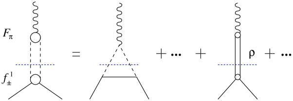
Figure 1: Two–pion contribution to the isovector nucleon form factors. On the left side, the exact representation based on unitarity is shown, whereas the triangle diagram on the right side leads to the strong enhancement of the isovector spectral functions close to threshold. Also shown is the dominant $\rho$–meson contribution.

We stress that the representation of Eq. (9) gives the exact isovector spectral functions for $4M_{\pi}^{2}\leq t\leq 16M_{\pi}^{2}$ but in practice holds up to $t\simeq 50M_{\pi}^{2}$. It has two distinct features. First, as already pointed out in [12], it contains the important contribution of the $\rho$ meson (see Fig. 1) with its peak at $t\simeq 30M_{\pi}^{2}$. Second, on the left shoulder of the $\rho$, the isovector spectral functions display a very pronounced enhancement close to the two–pion threshold. This is due to the logarithmic singularity on the second Riemann sheet located at $t_{c}=4M_{\pi}^{2}-M_{\pi}^{4}/m^{2}=3.98M_{\pi}^{2}$, very close to the threshold. This pole comes from the projection of the nucleon Born graphs, or in modern language, from the triangle diagram also depicted in Fig. 1. If one were to neglect this important unitarity correction, one would severely underestimate the nucleon isovector radii [16]. In fact, precisely the same effect is obtained at leading one–loop accuracy in chiral perturbation theory, as discussed first in [3, 26]. This topic was further elaborated on in the framework of heavy baryon CHPT [5, 10] and in a covariant calculation based on infrared regularization [8]. Thus, the most important two–pion contribution to the nucleon form factors can be determined by using either unitarity or CHPT (in the latter case, of course, the $\rho$ contribution is not included).

We now want to separate the (uncorrelated) pion contribution from the $\rho$–contribution in the isovector spectral functions, that is we decompose the isovector spectral functions as

$${\rm Im}~{}G_{I}^{V}(t)={\rm Im}~{}G_{I}^{V,2\pi}(t)+{\rm Im}~{}G_{I}^{V,\rho}(t)~{},\quad I=E,M~{},$$ (10)

and analogously for Im $F_{1,2}^{V}(t)$. Using Eq. (8), we can then calculate the pion cloud contribution to the charge and magnetization density in the Breit–frame. The $\rho$–contribution in Eq. (10) can be well represented by a Breit–Wigner form with a running width [10],

$${\rm Im}~{}G^{V,\rho}_{I}(t)=\frac{b_{I}M_{\rho}^{2}\sqrt{t}\Gamma_{\rho}(t)}{(M_{\rho}^{2}-t)^{2}+t\Gamma_{\rho}^{2}(t)}~{},\quad I=E,M~{},$$ (11)

with the mass $M_{\rho}=769.3\,$MeV and the width $\Gamma_{\rho}(t)=g^{2}(t-4M_{\pi}^{2})^{3/2}/(48\pi t)$, where the coupling $g=6.03$ is determined from the empirical value $\Gamma_{\rho}(M_{\rho}^{2})=150.2\,$ MeV, and the parameters $b_{I}$ can be adjusted to the height of the resonance peak. The corresponding expressions for the imaginary parts of the Dirac and Pauli form factors can be obtained from Eq. (4). It is clear that the separation into the (uncorrelated) pion contribution and the $\rho$–contribution introduces some model–dependence. To get an idea about the theoretical error induced by this procedure, we perform the separation in three different ways:

• The two–pion contribution can be directly obtained from the two–loop chiral perturbation theory calculation of [10]. Together with the $\rho$–contribution of Eq. (11), this calculation gives a very good description of the empirical spectral functions. We will use the analytical formulae given in [10] where the low–energy constant $c_{4}$ was readjusted to avoid double counting of the $\rho$–contribution (see [28]).

• A lower bound on the two–pion contribution can be obtained by setting $F_{\pi}(t)=1$ in Eq. (9). This prescription does not only remove the $\rho$–pole but also some small uncorrelated two–pion contributions contained in the pion form factor.

• To obtain the two–pion contribution, we can also subtract Eq. (11) from the spectral function Eq. (9) including the full pion form factor. The parameters $b_{E}=1.512$ and $b_{M}=5.114$ are determined such that the two–pion contribution at the $\rho$–resonance matches the two–loop chiral perturbation theory calculation of [10]. Variation of the $b_{I}$ around these values gives an additional error estimate.

Using these three methods, we obtain a fairly good handle on the theoretical accuracy of the non-resonant two–pion contribution.

4. We have now collected all pieces to work out the density distribution of the two–pion contribution to the nucleon electromagnetic form factors. Before showing the results, some remarks are in order. As stated above, the spectral functions are determined by unitarity (or chiral perturbation theory) only up to some maximum value of $t$, denoted $t_{\rm max}$ in the following. Thus, we have simply set the spectral functions in the integral Eq. (8) to zero for momentum transfers beyond the value $t_{\rm max}=40M_{\pi}^{2}$.

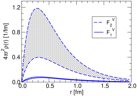
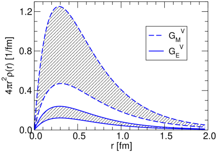
Figure 2: The densities of charge and magnetization due to the pion cloud. Left panel: $4\pi r^{2}\rho(r)$ for the isovector Pauli (upper band) and Dirac (lower band) form factors. Right panel: $4\pi r^{2}\rho(r)$ for the isovector magnetic (upper band) and electric (lower band) Sachs form factors.

In Fig. 2, we show the resulting densities for the isovector form factors weighted with $4\pi r^{2}$. The contribution of the “pion cloud” to the total charge or magnetic moment is then simply obtained by integration over $r$. The bands reflect the theoretical uncertainty in the separation. For all form factors, the lower and upper bounds are given by methods (b) and (a), respectively. Method (c) generally yields a result between these bounds, except for the Dirac form factor where it gives the upper bound. The weighted densities for the isovector Dirac and Pauli form factors are shown in the left panel of Fig. 2. We see that these charge distributions show a pronounced peak around $r\simeq 0.3\,$fm, quite consistent with earlier determinations (see e.g. [24, 29]), and fall off smoothly with increasing distance. In the right panel of Fig. 2, we show the densities (again weighted with $4\pi r^{2}$) for the electric and magnetic Sachs form factors which come out very similar to the case of the Dirac and Pauli form factors. In comparison with Ref. [23], we generally obtain much smaller pion cloud effects at distances beyond 1 fm, e.g., by a factor 3 for $\rho_{E}^{V}(r)$ at $r=1.5$ fm.

We have also studied the sensitivity of our results to the cut–off $t_{\rm{max}}$. While this may increase the value of the “pion cloud” contribution, it leaves the position of the maximum essentially unchanged. However, it is obvious from Eq. (8) that masses beyond 1 GeV and corresponding small–distance phenomena ($r\lesssim 0.2$ fm) should not be related to the pion cloud of the nucleon. Finally, we show the corresponding two–pion contribution to the charges and radii for the various nucleon form factors in Table 1. The contribution of the pion cloud to the isovector electric (magnetic) charge is 20% (10%) in the model of Ref. [23]. This is consistent with our range of values for the electric charge but a factor of 1.5 smaller than our lower bound for the magnetic one, see Table 1. Furthermore, note that the pion cloud gives only a fraction of all form factors at zero momentum transfer. Normalized to the contribution of the pion cloud, the corresponding radii are of the order of 1 fm. In the model of [23], these radii are considerably larger, of the order of 1.5 fm. Note that if one shifts all the strength of the corresponding spectral functions to threshold, one obtains an upper limit $r_{\rm max}=\sqrt{3/2}\,M_{\pi}^{-1}\simeq 1.7\,$fm, assuming that the spectral functions are positive definite.

$F_{1}^{V}(0)$	$F_{2}^{V}(0)$	$G_{E}^{V}(0)$	$G_{M}^{V}(0)$	$\langle r^{2}\rangle_{1}^{V}$	$\langle r^{2}\rangle_{2}^{V}$	$\langle r^{2}\rangle_{E}^{V}$	$\langle r^{2}\rangle_{M}^{V}$
$0.07...0.08$	$0.4...1.0$	$0.1...0.2$	$0.4...1.0$	$0.1...0.2$	$0.2...0.3$	$0.2...0.3$	$0.2...0.3$

Table 1: Two–pion contribution to charges and radii (in fm²) for the various nucleon form factors. The radii are normalized to the physical charges and magnetic moments.

5. In this letter, we have considered the two–pion contribution to the nucleon isovector form factors. The corresponding spectral functions can be obtained from unitarity or chiral perturbation theory from threshold $t_{0}=4M_{\pi}^{2}$ up to $t_{\rm max}\simeq 40M_{\pi}^{2}$ in a model–independent way. Subtracting the contribution from the dominant $\rho$–meson pole, we have constructed the uncorrelated two–pion component (loosely spoken the dominant effects of the nucleons’ pion cloud). To obtain an estimate about the theoretical error of such a procedure, we have performed this subtraction in three different ways. The corresponding charge densities obtained by Fourier transforming the spectral functions peak at distances of about 0.3 fm and show no structure at the larger distances.

Acknowledgements
We thank J. Friedrich and Th. Walcher as well as N. Kaiser for useful discussions. This work was supported in part by the Deutsche Forschungsgemeinschaft (SFB 443).

References

- [1]
- [2] H. Fröhlich, W. Heitler and N. Kemmer, Proc. Roy. Soc. A 166 (1938) 155.
- [3] J. Gasser, M. E. Sainio and A. Svarc, Nucl. Phys. B 307 (1988) 779.
- [4] V. Bernard, N. Kaiser, J. Kambor and U. G. Meissner, Nucl. Phys. B 388 (1992) 315.
- [5] V. Bernard, N. Kaiser and U.-G. Meißner, Nucl. Phys. A 611 (1996) 429 [arXiv:hep-ph/9607428].
- [6] H. W. Fearing, R. Lewis, N. Mobed and S. Scherer, Phys. Rev. D 56 (1997) 1783 [arXiv:hep-ph/9702394].
- [7] V. Bernard, H. W. Fearing, T. R. Hemmert and U.-G. Meißner, Nucl. Phys. A 635 (1998) 121 [Erratum-ibid. A 642 (1998) 563] [arXiv:hep-ph/9801297].
- [8] B. Kubis and U.-G. Meißner, Nucl. Phys. A 679 (2001) 698 [arXiv:hep-ph/0007056].
- [9] B. Kubis and U.-G. Meißner, Eur. Phys. J. C 18 (2001) 747 [arXiv:hep-ph/0010283].
- [10] N. Kaiser, Phys. Rev. C 68 (2003) 025202 [arXiv:nucl-th/0302072].
- [11] T. Fuchs, J. Gegelia and S. Scherer, arXiv:nucl-th/0305070.
- [12] W. R. Frazer and J. R. Fulco, Phys. Rev. Lett. 2 (1959) 365.
- [13] J. J. Sakurai, Ann. Phys. (NY) 11 (1960) 1.
- [14] G. J. Gounaris and J. J. Sakurai, Phys. Rev. Lett. 21 (1968) 244.
- [15] G. Höhler and E. Pietarinen, Nucl. Phys. B 95 (1975) 210.
- [16] G. Höhler and E. Pietarinen, Phys. Lett. B 53 (1975) 471.
- [17] M. Gari and W. Krümpelmann, Z. Phys. A 322 (1985) 689.
- [18] P. Mergell, U.-G. Meißner and D. Drechsel, Nucl. Phys. A 596 (1996) 367 [arXiv:hep-ph/9506375].
- [19] H. W. Hammer, U.-G. Meißner and D. Drechsel, Phys. Lett. B 385 (1996) 343 [arXiv:hep-ph/9604294].
- [20] E. L. Lomon, Phys. Rev. C 64 (2001) 035204 [arXiv:nucl-th/0104039].
- [21] S. Dubnicka, A. Z. Dubnickova and P. Weisenpacher, J. Phys. G 29 (2003) 405 [arXiv:hep-ph/0208051].
- [22] V. Bernard, T. R. Hemmert and U.-G. Meißner, arXiv:hep-ph/0307115, Nucl. Phys. A (2004) in press.
- [23] J. Friedrich and T. Walcher, Eur. Phys. J. A 17 (2003) 607 [arXiv:hep-ph/0303054].
- [24] U.-G. Meißner, Phys. Rept. 161 (1988) 213.
- [25] G. Höhler, ”Pion-Nucleon Scattering”, Landolt-Börnstein Vol. I/9b, ed. H. Schopper, Springer, Berlin, 1983.
- [26] V. Bernard, N. Kaiser and U.-G. Meißner, Int. J. Mod. Phys. E 4 (1995) 193 [arXiv:hep-ph/9501384].
- [27] U.-G. Meißner, Comm. Nucl. Part. Phys. 20 (1991) 119.
- [28] V. Bernard, N. Kaiser and U.-G. Meißner Nucl. Phys. A 615 (1997) 483 [arXiv:hep-ph/9611253].
- [29] G. Holzwarth, Z. Phys. A 356 (1996) 339 [arXiv:hep-ph/9606336].
- [30] M. K. Jones et al. [Jefferson Lab Hall A Collaboration], Phys. Rev. Lett. 84 (2000) 1398 [arXiv:nucl-ex/9910005].
- [31] O. Gayou et al. [Jefferson Lab Hall A Collaboration], Phys. Rev. Lett. 88 (2002) 092301 [arXiv:nucl-ex/0111010].