hep-ph/0310238

1 Introduction

The last five years have seen enormous progress in our knowledge of neutrino physics. We have now strong experimental evidences of the existence of neutrino oscillations, predicted by Pontecorvo in the late 50’s [1, 2], which occur if neutrinos are massive and mixed particles.

In 1998 the Super-Kamiokande experiment [3] provided a model-independent proof of the oscillations of atmospheric muon neutrinos, which were discovered in 1988 by the Kamiokande [4] and IMB [5] experiments. The values of the neutrino mixing parameters that generate atmospheric neutrino oscillations have been confirmed at the end of 2002 by the first results of the K2K long-baseline accelerator experiment [6], which observed a disappearance of muon neutrinos due to oscillations.

In 2001 the combined results of the SNO [7] and Super-Kamiokande [8] experiments gave a model-independent indication of the oscillations of solar electron neutrinos, which were discovered in the late 60’s by the Homestake experiment [9]. In 2002 the SNO experiment [10] measured the total flux of active neutrinos from the sun, providing a model-independent evidence of oscillations of electron neutrinos into other flavors, which has been confirmed with higher precision by recent data [11]. The values of the neutrino mixing parameters indicated by solar neutrino data have been confirmed at the end of 2002 by the KamLAND very-long-baseline reactor experiment [12], which have measured a disappearance of electron antineutrinos due to oscillations.

In this paper we review the currently favored scenario of three-neutrino mixing, which is based on the above mentioned evidences of neutrino oscillations. In Section 2 we review the theory of neutrino masses and mixing, showing that it is likely that massive neutrinos are Majorana particles. In Section 3 we review the theory of neutrino oscillations in vacuum and in matter. In Section 4 we review the main results of neutrino oscillation experiments. In Section 5 we discuss the main aspects of the phenomenology of three-neutrino mixing, including neutrino oscillations, experiments on the measurement of the absolute scale of neutrino masses and neutrinoless double-$\beta$ decay experiments searching for an evidence of the Majorana nature of massive neutrinos. In Section 6 we discuss some future prospects and in Section 7 we draw our conclusions.

For further information on the physics of massive neutrinos, see the books in Refs. [13, 14, 15], the reviews in Refs. [16, 17, 18, 19, 20, 21, 22, 23, 24, 25, 26, 27, 26, 28, 29, 30, 31, 32, 33, 34, 35, 36, 37, 38] and the references in Ref. [39].

2 Neutrino masses and mixing

The Standard Model was formulated in the 60’s [40, 41, 42] on the basis of the knowledge available at that time on the existing elementary particles and their properties. In particular, neutrinos were though to be massless following the so-called two-component theory of Landau [43], Lee and Yang [44], and Salam [45], in which the massless neutrinos are described by left-handed Weyl spinors. This description has been reproduced in the Standard Model of Glashow [40], Weinberg [41] and Salam [42] assuming the non existence of right-handed neutrino fields, which are necessary in order to generate Dirac neutrino masses with the same Higgs mechanism that generates the Dirac masses of quarks and charged leptons. However, as will be discussed in Section 4, in recent years neutrino experiments have shown convincing evidences of the existence of neutrino oscillations, which is a consequence of neutrino masses and mixing. Hence, it is time to revise the Standard Model in order to take into account neutrino masses (notice that the Standard Model has already been revised in the early 70’s with the inclusion first of the charmed quark and after of the third generation).

2.1 Dirac mass term

Considering for simplicity only one neutrino field $\nu$, the standard Higgs mechanism generates the Dirac mass term

$$\mathcal{L}^{\text{D}}=-m_{\text{D}}\,\overline{\nu}\,\nu=-m_{\text{D}}\left(\overline{\nu_{R}}\,\nu_{L}+\overline{\nu_{L}}\,\nu_{R}\right)\,,$$ (2.1)

with $m_{\text{D}}=y\,v/\sqrt{2}$ where $y$ is a dimensionless Yukawa coupling coefficient and $v/\sqrt{2}$ is the Vacuum Expectation Value of the Higgs field. $\nu_{L}$ and $\nu_{R}$ are, respectively, the chiral left-handed and right-handed components of the neutrino field, obtained by acting on $\nu$ with the corresponding projection operator:

$$\nu=\nu_{L}+\nu_{R}\,,\quad\nu_{L}=P_{L}\,\nu\,,\quad\nu_{R}=P_{R}\,\nu\,,\quad P_{L}\equiv\frac{1-\gamma^{5}}{2}\,,\quad P_{R}\equiv\frac{1+\gamma^{5}}{2}\,,$$ (2.2)

such that $P_{L}P_{R}=P_{R}P_{L}=0$, $P_{L}^{2}=P_{L}$, $P_{R}^{2}=P_{R}$, since $(\gamma^{5})^{2}=1$. Therefore, we have

$$P_{L}\,\nu_{L}=\nu_{L}\,,\quad P_{L}\,\nu_{R}=0\,,\quad P_{R}\,\nu_{L}=0\,,\quad P_{R}\,\nu_{R}=\nu_{R}\,.$$ (2.3)

It can be shown that the chiral spinors $\nu_{L}$ and $\nu_{R}$ have only two independent components each, leading to the correct number of four for the independent components of the spinor $\nu$.

Unfortunately, the generation of Dirac neutrino masses through the standard Higgs mechanism is not able to explain naturally why the neutrino are more than five order of magnitude lighter than the electron, which is the lightest of the other elementary particles (as discussed in Section 4, the neutrino masses are experimentally constrained below about 1-2 eV). In other words, there is no explanation of why the neutrino Yukawa coupling coefficients are more than five order of magnitude smaller than the Yukawa coupling coefficients of quarks and charged leptons.

2.2 Majorana mass term

In 1937 Majorana [46] discovered that a massive neutral fermion as a neutrino can be described by a spinor $\psi$ with only two independent components imposing the so-called Majorana condition

$$\psi=\psi^{c}\,,$$ (2.4)

where $\psi^{c}=\mathcal{C}\overline{\psi}^{T}=\mathcal{C}{\gamma^{0}}^{T}\psi^{*}$ is the operation of charge conjugation, with the charge-conjugation matrix $\mathcal{C}$ defined by the relations $\mathcal{C}{\gamma^{\mu}}^{T}\mathcal{C}^{-1}=-\gamma^{\mu}$, $\mathcal{C}^{\dagger}=\mathcal{C}^{-1}$, $\mathcal{C}^{T}=-\mathcal{C}$. Since $\mathcal{C}{\gamma^{5}}^{T}\mathcal{C}^{-1}=\gamma^{5}$ and $\gamma^{5}\gamma^{\mu}+\gamma^{\mu}\gamma^{5}=0$, we have

$$P_{L}\,\psi_{L}^{c}=0\,,\quad P_{L}\,\psi_{R}^{c}=\psi_{R}^{c}\,,\quad P_{R}\,\psi_{L}^{c}=\psi_{L}^{c}\,,\quad P_{R}\,\psi_{R}^{c}=0\,.$$ (2.5)

In other words, $\psi_{L}^{c}$ is right-handed and $\psi_{R}^{c}$ is left-handed.

Decomposing the Majorana condition (2.4) into left-handed and right-handed components, $\psi_{L}+\psi_{R}=\psi_{L}^{c}+\psi_{R}^{c}$, and acting on both members of the equation with the right-handed projector operator $P_{R}$, we obtain

$$\psi_{R}=\psi_{L}^{c}\,.$$ (2.6)

Thus, the right-handed component $\psi_{R}$ of the Majorana neutrino field $\psi$ is not independent, but obtained from the left-handed component $\psi_{L}$ through charge conjugation and the Majorana field can be written as

$$\psi=\psi_{L}+\psi_{L}^{c}\,.$$ (2.7)

This field depends only on the two independent components of $\psi_{L}$. Using the constraint (2.6) in the mass term (2.1), we obtain the Majorana mass term

$$\mathcal{L}^{\text{M}}=-\frac{1}{2}\,m_{\text{M}}\left(\overline{\psi_{L}^{c}}\,\psi_{L}+\overline{\psi_{L}}\,\psi_{L}^{c}\right)\,,$$ (2.8)

where we have inserted a factor $1/2$ in order to avoid double counting in the Euler-Lagrange derivation of the equation for the Majorana neutrino field.

2.3 Dirac-Majorana mass term

In general, if both the chiral left-handed and right-handed fields exist and are independent, in addition to the Dirac mass term (2.1) also the Majorana mass terms for $\nu_{L}$ and $\nu_{R}$ are allowed:

$$\mathcal{L}^{\text{M}}_{L}=-\frac{1}{2}\,m_{L}\left(\overline{\nu_{L}^{c}}\,\nu_{L}+\overline{\nu_{L}}\,\nu_{L}^{c}\right)\,,\qquad\mathcal{L}^{\text{M}}_{R}=-\frac{1}{2}\,m_{R}\left(\overline{\nu_{R}^{c}}\,\nu_{R}+\overline{\nu_{R}}\,\nu_{R}^{c}\right)\,.$$ (2.9)

The total Dirac+Majorana mass term

$$\mathcal{L}^{\text{D+M}}=\mathcal{L}^{\text{D}}+\mathcal{L}^{\text{M}}_{L}+\mathcal{L}^{\text{M}}_{R}$$ (2.10)

can be written as

$$\mathcal{L}^{\text{D+M}}=-\frac{1}{2}\begin{pmatrix}\overline{\nu_{L}^{c}}&\overline{\nu_{R}}\end{pmatrix}\begin{pmatrix}m_{L}&m_{\text{D}}\\ m_{\text{D}}&m_{R}\end{pmatrix}\begin{pmatrix}\nu_{L}\\ \nu_{R}^{c}\end{pmatrix}+\text{H.c.}\,.$$ (2.11)

It is clear that the chiral fields $\nu_{L}$ and $\nu_{R}$ do not have a definite mass, since they are coupled by the Dirac mass term. In order to find the fields with definite masses it is necessary to diagonalize the mass matrix in Eq. (2.11). For this task, it is convenient to write the Dirac+Majorana mass term in the matrix form

$$\mathcal{L}^{\text{D+M}}=\frac{1}{2}\,\overline{N_{L}^{c}}\,M\,N_{L}+\text{H.c.}\,,$$ (2.12)

with the matrices

$$M=\begin{pmatrix}m_{L}&m_{\text{D}}\\ m_{\text{D}}&m_{R}\end{pmatrix}\,,\qquad N_{L}=\begin{pmatrix}\nu_{L}\\ \nu_{R}^{c}\end{pmatrix}\,.$$ (2.13)

The column matrix $N_{L}$ is left-handed, because it contains left-handed fields. Let us write it as

$$N_{L}=U\,n_{L}\,,\qquad\text{with}\qquad n_{L}=\begin{pmatrix}\nu_{1L}\\ \nu_{2L}\end{pmatrix}\,,$$ (2.14)

where $U$ is the unitary mixing matrix ($U^{\dagger}=U^{-1}$) and $n_{L}$ is the column matrix of the left-handed components of the massive neutrino fields. The Dirac+Majorana mass term is diagonalized requiring that

$$U^{T}\,M\,U=\begin{pmatrix}m_{1}&0\\ 0&m_{2}\end{pmatrix}\,,$$ (2.15)

with $m_{k}$ real and positive for $k=1,2$.

Let us consider the simplest case of a real mass matrix $M$. Since the values of $m_{L}$ and $m_{R}$ can be chosen real and positive by an appropriate choice of phase of the chiral fields $\nu_{L}$ and $\nu_{R}$, the mass matrix $M$ is real if $m_{\text{D}}$ is real. In this case, the mixing matrix $U$ can be written as

$$U=\mathcal{O}\,\rho\,,$$ (2.16)

where $\mathcal{O}$ is an orthogonal matrix and $\rho$ is a diagonal matrix of phases:

$$\mathcal{O}=\begin{pmatrix}\cos\vartheta&\sin\vartheta\\ -\sin\vartheta&\cos\vartheta\end{pmatrix}\,,\qquad\rho=\begin{pmatrix}\rho_{1}&0\\ 0&\rho_{2}\end{pmatrix}\,,$$ (2.17)

with $|\rho_{k}|^{2}=1$. The orthogonal matrix $\mathcal{O}$ is chosen in order to have

$$\mathcal{O}^{T}\,M\,\mathcal{O}=\begin{pmatrix}m^{\prime}_{1}&0\\ 0&m^{\prime}_{2}\end{pmatrix}\,,$$ (2.18)

leading to

$$\tan 2\vartheta=\frac{2m_{\text{D}}}{m_{R}-m_{L}}\,,\qquad m^{\prime}_{2,1}=\frac{1}{2}\left[m_{L}+m_{R}\pm\sqrt{\left(m_{L}-m_{R}\right)^{2}+4\,m_{\text{D}}^{2}}\right]\,.$$ (2.19)

Having chosen $m_{L}$ and $m_{R}$ positive, $m^{\prime}_{2}$ is always positive, but $m^{\prime}_{1}$ is negative if $m_{\text{D}}^{2}>m_{L}m_{R}$. Since

$$U^{T}\,M\,U=\rho^{T}\,\mathcal{O}^{T}\,M\,\mathcal{O}\,\rho=\begin{pmatrix}\rho_{1}^{2}\,m^{\prime}_{1}&0\\ 0&\rho_{2}^{2}\,m^{\prime}_{2}\end{pmatrix}\,,$$ (2.20)

it is clear that the role of the phases $\rho_{k}$ is to make the masses $m_{k}$ positive, as masses must be. Hence, we have $\rho_{2}^{2}=1$ always, and $\rho_{1}^{2}=1$ if $m^{\prime}_{1}\geq 0$ or $\rho_{1}^{2}=-1$ if $m^{\prime}_{1}<0$.

An important fact to be noticed is that the diagonalized Dirac+Majorana mass term,

$$\mathcal{L}^{\text{D+M}}=\frac{1}{2}\sum_{k=1,2}m_{k}\,\overline{\nu_{kL}^{c}}\,\nu_{kL}+\text{H.c.}\,,$$ (2.21)

is a sum of Majorana mass terms for the massive Majorana neutrino fields

$$\nu_{k}=\nu_{kL}+\nu_{kL}^{c}\qquad(k=1,2)\,.$$ (2.22)

Therefore, the two massive neutrinos are Majorana particles.

2.4 The see-saw mechanism

It is possible to show that the Dirac+Majorana mass term leads to maximal mixing ($\theta=\pi/4$) if $m_{L}=m_{R}$, or to so-called pseudo-Dirac neutrinos if $m_{L}$ and $m_{R}$ are much smaller that $|m_{\text{D}}|$ (see Ref. [21]). However, the most plausible and interesting case is the so-called see-saw mechanism [47, 48, 49], which is obtained considering $m_{L}=0$ and $|m_{\text{D}}|\ll m_{R}$. In this case

$$m_{1}\simeq\frac{(m_{\text{D}})^{2}}{m_{R}}\ll|m_{\text{D}}|\,,\qquad m_{2}\simeq m_{R}\,,\qquad\tan\vartheta\simeq\frac{m_{\text{D}}}{m_{R}}\ll 1\,,\qquad\rho_{1}^{2}=-1\,.$$ (2.23)

What is interesting in Eq. (2.23) is that $m_{1}$ is much smaller than $m_{\text{D}}$, being suppressed by the small ratio $m_{\text{D}}/m_{R}$. Since $m_{2}$ is of order $m_{R}$, a very heavy $\nu_{2}$ corresponds to a very light $\nu_{1}$, as in a see-saw. Since $m_{\text{D}}$ is a Dirac mass, presumably generated with the standard Higgs mechanism, its value is expected to be of the same order as the mass of a quark or the charged fermion in the same generation of the neutrino we are considering. Hence, the see-saw explains naturally the suppression of $m_{1}$ with respect to $m_{\text{D}}$, providing the most plausible explanation of the smallness of neutrino masses.

The smallness of the mixing angle $\vartheta$ in Eq. (2.23) implies that $\nu_{1L}\simeq-\nu_{L}$ and $\nu_{2L}\simeq\nu_{R}^{c}$. This means that the neutrino participating to weak interactions practically coincides with the light neutrino $\nu_{1}$, whereas the heavy neutrino $\nu_{2}$ is practically decoupled from interactions with matter.

Besides the smallness of the light neutrino mass, another important consequence of the see-saw mechanism is that massive neutrinos are Majorana particles, as we have shown above in the general case of a Dirac+Majorana mass term. This is a very important indication that strongly encourages the search for the Majorana nature of neutrinos, mainly performed through the search of neutrinoless double-$\beta$ decay.

An important assumption necessary for the see-saw mechanism is $m_{L}=0$. Such assumption may seem arbitrary at first sight, but in fact it is not. Its plausibility follows from the fact that $\nu_{L}$ belongs to a weak isodoublet of the Standard Model:

$$L_{L}=\begin{pmatrix}\nu_{L}\\ \ell_{L}\end{pmatrix}\,.$$ (2.24)

Since $\nu_{L}$ has third component of the weak isospin $I_{3}=1/2$, the combination $\overline{\nu_{L}^{c}}\nu_{L}=-\nu_{L}^{T}\mathcal{C}^{\dagger}\nu_{L}$ in the Majorana mass term in Eq. (2.9) has $I_{3}=1$ and belongs to a triplet. Since in the Standard Model there is no Higgs triplet that could couple to $\overline{\nu_{L}^{c}}\nu_{L}$ in order to form a Lagrangian term invariant under a SU(2)_L transformation of the Standard Model gauge group, a Majorana mass term for $\nu_{L}$ is forbidden. In other words, the gauge symmetries of the Standard Model imply $m_{L}=0$, as needed for the see-saw mechanism. On the other hand, $m_{\text{D}}$ is allowed in the Standard Model, because it is generated through the standard Higgs mechanism, and $m_{R}$ is also allowed, because $\nu_{R}$ and $\overline{\nu_{R}^{c}}\nu_{R}$ are singlets of the Standard Model gauge symmetries. Hence, quite unexpectedly, we have an extended Standard Model with massive neutrinos that are Majorana particles and in which the smallness of neutrino masses can be naturally explained through the see-saw mechanism.

The only assumption which remains unexplained in this scenario is the heaviness of $m_{R}$ with respect to $m_{\text{D}}$. This assumption cannot be motivated in the framework of the Standard Model, because $m_{R}$ is only a parameter which could have any value. However, there are rather strong arguments that lead us to believe that the Standard Model is a theory that describes the world only at low energies. In this case it is natural to expect that the mass $m_{R}$ is generated at ultra-high energy by the symmetry breaking of the theory beyond the Standard Model. Hence, it is plausible that the value of $m_{R}$ is many orders of magnitude larger than the scale of the electroweak symmetry breaking and of $m_{\text{D}}$, as required for the working of the see-saw mechanism.

2.5 Effective dimension-five operator

If we consider the possibility of a theory beyond the Standard Model, another question regarding the neutrino masses arises: is it possible that a Lagrangian term exists at the high energy of the theory beyond the Standard Model which generates at low energy an effective Majorana mass term for $\nu_{L}$? The answer is yes [50, 51, 52]: the operator with lowest dimension invariant under $\text{SU}(2)_{L}\times\text{U}(1)_{Y}$ that can generate a Majorana mass term for $\nu_{L}$ after electroweak symmetry breaking is the dimension-five operator

$$\frac{g}{\mathcal{M}}(L_{L}^{T}\,\sigma_{2}\,\Phi)\,\mathcal{C}^{-1}\,(\Phi^{T}\,\sigma_{2}\,L_{L})+\text{H.c.}\,,$$ (2.25)

where $g$ is a dimensionless coupling coefficient and $\mathcal{M}$ is the high-energy scale at which the new theory breaks down to the Standard Model. The dimension-five operator in Eq. (2.25) does not belong to the Standard Model because it is not renormalizable. It must be considered as an effective operator which is the low-energy manifestation of the renormalizable new theory beyond the Standard Model, in analogy with the old non-renormalizable Fermi theory of weak interactions, which is the low-energy manifestation of the Standard Model.

At the electroweak symmetry breaking

$$\Phi=\begin{pmatrix}\phi^{+}\\ \phi^{0}\end{pmatrix}\ \xrightarrow{\text{Symmetry Breaking}}\ \begin{pmatrix}0\\ v/\sqrt{2}\end{pmatrix}\,,$$ (2.26)

the operator in Eq. (2.25) generates the Majorana mass term for $\nu_{L}$ in Eq. (2.9), with

$$m_{L}=\frac{g\,v^{2}}{\mathcal{M}}\,.$$ (2.27)

This relation is very important, because it shows that the Majorana mass $m_{L}$ is suppressed with respect to $v$ by the small ratio $v/\mathcal{M}$. In other words, since the Dirac mass term $m_{\text{D}}$ is equal to $v/\sqrt{2}$ times a Yukawa coupling coefficient, the relation (2.27) has a see-saw form. Therefore, the effect of the dimension-five effective operator in Eq. (2.25) does not spoil the natural suppression of the light neutrino mass provided by the see-saw mechanism. Indeed, considering $m_{L}\sim m_{\text{D}}^{2}/m_{R}$ and taking into account that $m_{1}=|m^{\prime}_{1}|$, from Eq. (2.19) we obtain

$$m_{1}\simeq\left|m_{L}-\frac{(m_{\text{D}})^{2}}{m_{R}}\right|\,.$$ (2.28)

Equations (2.27) and (2.28) show that the see-saw mechanism is operating even if $m_{L}$ is not zero, but it is generated by the dimension-five operator in Eq. (2.25). On the other hand, if the chiral right-handed neutrino field $\nu_{R}$ does not exist, the standard see-saw mechanism cannot be implemented, but a Majorana neutrino mass $m_{L}$ can be generated by the dimension-five operator in Eq. (2.25), and Eq. (2.27) shows that the suppression of the light neutrino mass is natural and of see-saw type.

2.6 Three-neutrino mixing

So far we have considered for simplicity only one neutrino, but it is well known from a large variety of experimental data that there are three neutrinos that participate to weak interactions: $\nu_{e}$, $\nu_{\mu}$, $\nu_{\tau}$. These neutrinos are called “active flavor neutrinos”. From the precise measurement of the invisible width of the $Z$-boson produced by the decays $\displaystyle Z\to\sum_{\alpha}\nu_{\alpha}\bar{\nu}_{\alpha}$ we also know that the number of active flavor neutrinos is exactly three (see Ref. [53]), excluding the possibility of existence of additional heavy active flavor neutrinos. The active flavor neutrinos take part in the charged-current (CC) and neutral current (NC) weak interaction Lagrangians

$$\mathcal{L}_{I}^{\text{CC}}=-\frac{g}{2\sqrt{2}}\,j^{\text{CC}}_{\rho}\,W^{\rho}+\text{H.c.}\,,\hbox{} \hbox{}\quad\text{with}\quad j^{\text{CC}}_{\rho}=2\sum_{\alpha=e,\mu,\tau}\overline{\nu_{\alpha L}}\,\gamma_{\rho}\,\alpha_{L}\,,$$ (2.29)

$$\mathcal{L}_{I}^{\text{NC}}=-\frac{g}{2\cos{\vartheta_{\text{W}}}}\,j^{\text{NC}}_{\rho}\,Z^{\rho}\,,\hbox{} \hbox{}\quad\text{with}\quad j^{\text{NC}}_{\rho}=\sum_{\alpha=e,\mu,\tau}\overline{\nu_{\alpha L}}\,\gamma_{\rho}\,\nu_{\alpha L}\,,$$ (2.30)

where $j^{\text{CC}}_{\rho}$ and $j^{\text{NC}}_{\rho}$ are, respectively, the charged and neutral leptonic currents, $\vartheta_{\text{W}}$ is the weak mixing angle ($\sin^{2}\vartheta_{\text{W}}\simeq 0.23$) and $g=e/\sin\vartheta_{\text{W}}$ ($e$ is the positron electric charge).

Let us consider three left-handed chiral fields $\nu_{eL}$, $\nu_{\mu L}$, $\nu_{\tau L}$ that describe the three active flavor neutrinos and three corresponding right-handed chiral fields $\nu_{s_{1}R}$, $\nu_{s_{2}R}$, $\nu_{s_{3}R}$ that describe three sterile neutrinos, which do not take part in weak interactions. The corresponding Dirac+Majorana mass term is given by Eq. (2.10) with

$$\hbox{}\mathcal{L}^{\text{D}}=-\sum_{s,\beta}\overline{\nu_{sR}}\,M^{\text{D}}_{s\beta}\,\nu_{\beta L}+\text{H.c.}\,,$$ (2.31)

$$\hbox{}\mathcal{L}^{\text{M}}_{L}=-\frac{1}{2}\sum_{\alpha,\beta}\overline{\nu_{{\alpha}L}^{c}}\,M^{L}_{\alpha\beta}\,\nu_{{\beta}L}+\text{H.c.}\,,$$ (2.32)

$$\hbox{}\mathcal{L}^{\text{M}}_{R}=-\frac{1}{2}\sum_{s,s^{\prime}}\overline{\nu_{sR}^{c}}\,M^{R}_{\alpha\beta}\,\nu_{s^{\prime}R}+\text{H.c.}\,,$$ (2.33)

where $M^{\text{D}}$ is a complex matrix and $M^{L}$, $M^{R}$ are symmetric complex matrices. The Dirac+Majorana mass term can be written as the one in Eq. (2.12) with the column matrix of left-handed fields

$$N_{L}=\begin{pmatrix}\nu_{L}\\ \displaystyle\nu_{R}^{c}\end{pmatrix}\,,\qquad\text{with}\qquad\nu_{L}=\begin{pmatrix}\nu_{eL}\\ \displaystyle\nu_{{\mu}L}\\ \displaystyle\nu_{{\tau}L}\end{pmatrix}\qquad\text{and}\qquad\nu_{R}^{c}=\begin{pmatrix}\nu_{s_{1}R}^{c}\\ \displaystyle\nu_{s_{2}R}^{c}\\ \displaystyle\nu_{s_{3}R}^{c}\end{pmatrix}\,,$$ (2.34)

and the $6\times 6$ mass matrix

$$M=\begin{pmatrix}M^{L}&(M^{\text{D}})^{T}\\ \displaystyle M^{\text{D}}&M^{R}\end{pmatrix}\,.$$ (2.35)

The mass matrix is diagonalized by a unitary transformation analogous to the one in Eq. (2.14):

$$N_{L}=\mathbb{V}\,n_{L}\,,\qquad\text{with}\qquad n_{L}=\begin{pmatrix}\nu_{1L}\\ \vdots\\ \nu_{6L}\end{pmatrix}\,,$$ (2.36)

where $\mathbb{V}$ is the unitary $6\times 6$ mixing matrix and $n_{kL}$ are the left-handed components of the massive neutrino fields. The mixing matrix $\mathbb{V}$ is determined by the diagonalization relation

$$\mathbb{V}^{T}\,M\,\mathbb{V}=\text{diag}\!\left(m_{1},\ldots,m_{6}\right)\,,$$ (2.37)

with $m_{k}$ real and positive for $k=1,\ldots,6$ (see Ref. [17] for a proof that it can be done). After diagonalization the Dirac+Majorana mass term is written as

$$\mathcal{L}^{\text{D+M}}=-\frac{1}{2}\sum_{k=1}^{6}m_{k}\,\overline{\nu_{kL}^{c}}\,\nu_{kL}+\text{H.c.}\,,$$ (2.38)

which is a sum of Majorana mass terms for the massive Majorana neutrino fields

$$\nu_{k}=\nu_{kL}+\nu_{kL}^{c}\qquad(k=1,\ldots,6)\,.$$ (2.39)

Hence, as we have already seen in Section 2.3 in the case of one neutrino generation, a Dirac+Majorana mass term implies that massive neutrinos are Majorana particles. The mixing relation (2.36) can be written as

$$\nu_{{\alpha}L}=\sum_{k=1}^{6}\mathbb{V}_{{\alpha}k}\,\nu_{kL}\qquad(\alpha=e,\mu,\tau)\,,\qquad\nu_{sR}^{c}=\sum_{k=1}^{6}\mathbb{V}_{sk}\,\nu_{kL}\qquad(s=s_{1},s_{2},s_{3})\,,$$ (2.40)

which shows that active and sterile neutrinos are linear combinations of the same massive neutrino fields. This means that in general active-sterile oscillations are possible (see Section 3).

The most interesting possibility offered by the Dirac+Majorana mass term is the implementation of the see-saw mechanism for the explanation of the smallness of the light neutrino masses, which is however considerably more complicated than in the case of one generation discussed in Section 2.4. Let us assume that $M^{L}=0$, in compliance with the gauge symmetries of the Standard Model and the absence of a Higgs triplet. Let us further assume that the eigenvalues of $M^{R}$ are much larger than those of $M^{\text{D}}$, as expected if the Majorana mass term (2.33) for the sterile neutrinos is generated at a very high energy scale characteristic of the theory beyond the Standard Model. In this case, we can write the mixing matrix $\mathbb{V}$ as

$$\mathbb{V}=\mathbb{W}\,\mathbb{U}\,,$$ (2.41)

where both $\mathbb{W}$ and $\mathbb{U}$ are unitary matrices, and use $\mathbb{W}$ for an approximate block-diagonalization of the mass matrix $M$ at leading order in the expansion in powers of $(M^{R})^{-1}M^{\text{D}}$:

$$\mathbb{W}^{T}\,M\,\mathbb{W}\simeq\begin{pmatrix}M_{\text{light}}&0\\ 0&M_{\text{heavy}}\end{pmatrix}\,.$$ (2.42)

The matrix $\mathbb{W}$ is given by

$$\mathbb{W}=1-\frac{1}{2}\begin{pmatrix}(M^{\text{D}})^{\dagger}(M^{R}{(M^{R})}^{\dagger})^{-1}M^{\text{D}}&2(M^{\text{D}})^{\dagger}{(M^{R})^{\dagger}}^{-1}\\ -2(M^{R})^{-1}M^{\text{D}}&(M^{R})^{-1}M^{\text{D}}(M^{\text{D}})^{\dagger}{(M^{R})^{\dagger}}^{-1}\end{pmatrix}\,,$$ (2.43)

and is unitary up to corrections of order $(M^{R})^{-1}M^{\text{D}}$. The two $3\times 3$ mass matrices $M_{\text{light}}$ and $M_{\text{heavy}}$ are given by

$$M_{\text{light}}\simeq-(M^{\text{D}})^{T}\,(M^{R})^{-1}\,M^{\text{D}}\,,\qquad M_{\text{heavy}}\simeq M^{R}\,.$$ (2.44)

Therefore, the see-saw mechanism is implemented by the suppression of $M_{\text{light}}$ with respect to $M^{\text{D}}$ by the small ratio $(M^{\text{D}})^{T}\,(M^{R})^{-1}$. The light and heavy mass sectors are practically decoupled because of the smallness of the off-diagonal $3\times 3$ block elements in Eq. (2.43).

For the low-energy phenomenology it is sufficient to consider only the light $3\times 3$ mass matrix $M_{\text{light}}$ which is diagonalized by the $3\times 3$ upper-left submatrix of $\mathbb{U}$ that we call $U$, such that

$$U^{T}\,M_{\text{light}}\,U=\text{diag}\!\left(m_{1},m_{2},m_{3}\right)\,,$$ (2.45)

where $m_{1},m_{2},m_{3}$ are the three light neutrino mass eigenvalues. Neglecting the small mixing with the heavy sector, the effective mixing of the active flavor neutrinos relevant for the low-energy phenomenology is given by

$$\nu_{{\alpha}L}=\sum_{k=1}^{3}U_{{\alpha}k}\,\nu_{kL}\qquad(\alpha=e,\mu,\tau)\,,$$ (2.46)

where $\nu_{1L}$, $\nu_{2L}$, $\nu_{3L}$ are the left-handed components of the three light massive Majorana neutrino fields. This scenario, called “three-neutrino mixing”, can accommodate the experimental evidences of neutrino oscillations in solar and atmospheric neutrino experiments reviewed in Section 4. The phenomenology of three-neutrino mixing is discussed in Section 5.

The $3\times 3$ unitary mixing matrix $U$ can be parameterized in terms of $3^{2}=9$ parameters which can be divided in $3$ mixing angles and $6$ phases. However, only $3$ phases are physical. This can be seen by considering the charged-current Lagrangian (2.29), which can be written as

$$\mathcal{L}_{I}^{\text{CC}}=-\frac{g}{\sqrt{2}}\sum_{\alpha=e,\mu,\tau}\sum_{k=1}^{3}\overline{\alpha_{L}}\,\gamma^{\rho}\,U_{\alpha k}\,\nu_{kL}\,W_{\rho}^{\dagger}+\text{H.c.}\,,$$ (2.47)

in terms of the light massive neutrino fields $\nu_{k}$ ($k=1,2,3$). Three of the six phases in $U$ can be eliminated by rephasing the charged lepton fields $e$, $\mu$, $\tau$, whose phases are arbitrary because all other terms in the Lagrangian are invariant under such change of phases (see Refs. [56, 57, 58] and the appendices of Refs. [59, 60]). On the other hand, the phases of the Majorana massive neutrino fields cannot be changed, because the Majorana mass term in Eq. (2.38) are not invariant under rephasing of $\nu_{kL}$. Therefore, the number of physical phases in the mixing matrix $U$ is three and it can be shown that two of these phases can be factorized in a diagonal matrix of phases on the right of $U$. These two phases are usually called “Majorana phases”, because they appear only if the massive neutrinos are Majorana particles (if the massive neutrinos are Dirac particles these two phases can be eliminated by rephasing the massive neutrino fields, since a Dirac mass term is invariant under rephasing of the fields). The third phase is usually called “Dirac phase”, because it is present also if the massive neutrinos are Dirac particles, being the analogous of the phase in the quark mixing matrix. These complex phases in the mixing matrix generate violations of the CP symmetry (see Refs. [13, 14, 17, 21]).

The most common parameterization of the mixing matrix is

$$U=\hbox{} \hbox{}R_{23}\,W_{13}\,R_{12}\,D(\lambda_{21},\lambda_{31})$$

$$=\hbox{} \hbox{}\begin{pmatrix}1&0&0\\ 0&c_{23}&s_{23}\\ 0&-s_{23}&c_{23}\end{pmatrix}\begin{pmatrix}c_{13}&0&s_{13}e^{-i\varphi_{13}}\\ 0&1&0\\ -s_{13}e^{i\varphi_{13}}&0&c_{13}\end{pmatrix}\begin{pmatrix}c_{12}&s_{12}&0\\ -s_{12}&c_{12}&0\\ 0&0&1\end{pmatrix}\begin{pmatrix}1&0&0\\ 0&e^{i\lambda_{21}}&0\\ 0&0&e^{i\lambda_{31}}\end{pmatrix}$$

$$=\hbox{} \hbox{}\begin{pmatrix}c_{12}c_{13}&s_{12}c_{13}&s_{13}e^{-i\varphi_{13}}\\ -s_{12}c_{23}-c_{12}s_{23}s_{13}e^{i\varphi_{13}}&c_{12}c_{23}-s_{12}s_{23}s_{13}e^{i\varphi_{13}}&s_{23}c_{13}\\ s_{12}s_{23}-c_{12}c_{23}s_{13}e^{i\varphi_{13}}&-c_{12}s_{23}-s_{12}c_{23}s_{13}e^{i\varphi_{13}}&c_{23}c_{13}\end{pmatrix}\begin{pmatrix}1&0&0\\ 0&e^{i\lambda_{21}}&0\\ 0&0&e^{i\lambda_{31}}\end{pmatrix}\,,$$ (2.48)

with $c_{ij}\equiv\cos\vartheta_{ij}$, $s_{ij}\equiv\sin\vartheta_{ij}$, where $\vartheta_{12}$, $\vartheta_{23}$, $\vartheta_{13}$ are the three mixing angles, $\varphi_{13}$ is the Dirac phase, $\lambda_{21}$ and $\lambda_{31}$ are the Majorana phases. In Eq. (2.48) $R_{ij}$ is a real rotation in the $i$-$j$ plane, $W_{13}$ is a complex rotation in the $1$-$3$ plane and $D(\lambda_{21},\lambda_{31})$ is the diagonal matrix with the Majorana phases.

Let us finally remark that, although in the case of Majorana neutrinos there is no difference between neutrinos and antineutrinos and one should only distinguish between states with positive and negative helicity, it is a common convention to call neutrino a particles created together with a positive charged lepton and having almost exactly negative helicity, and antineutrino a particles created together with a negative charged lepton and having almost exactly positive helicity. This convention follows from the fact that Dirac neutrinos are created together with a positive charged lepton and almost exactly negative helicity, and Dirac antineutrinos are created together with a negative charged lepton and almost exactly positive helicity.

3 Theory of neutrino oscillations

In order to derive neutrino oscillations it is useful to realize from the beginning that detectable neutrinos, relevant in oscillation experiments, are always ultrarelativistic particles. Indeed, as discussed in Section 4, the neutrino masses are experimentally constrained below about 1-2 eV, whereas only neutrinos more energetic than about 200 keV can be detected in:

1. Charged current weak processes which have an energy threshold larger than some fraction of MeV. For example:

   • $E_{\text{th}}=0.233\,\text{MeV}$ for $\nu_{e}+{}^{71}\text{Ga}\to{}^{71}\text{Ge}+e^{-}$ in the GALLEX [61], SAGE [62] and GNO [63] solar neutrino experiments.

   • $E_{\text{th}}=0.81\,\text{MeV}$ for $\nu_{e}+{}^{37}\text{Cl}\to{}^{37}\text{Ar}+e^{-}$ in the Homestake [9] solar neutrino experiment.

   • $E_{\text{th}}=1.8\,\text{MeV}$ for $\bar{\nu}_{e}+p\to n+e^{+}$ in reactor neutrino experiments (for example Bugey [64], CHOOZ [65] and KamLAND [12]).

2. The elastic scattering process $\nu+e^{-}\to\nu+e^{-}$, whose cross section is proportional to the neutrino energy ($\sigma(E)\sim\sigma_{0}E/m_{e}$, with $\sigma_{0}\sim 10^{-44}\,\text{cm}^{2}$). Therefore, an energy threshold of some MeV’s is needed in order to have a signal above the background. For example, $E_{\text{th}}\simeq 5\,\text{MeV}$ in the Super-Kamiokande [66, 67] solar neutrino experiment.

The comparison of the experimental limit on neutrino masses with the energy threshold in the processes of neutrino detection implies that detectable neutrinos are extremely relativistic.

3.1 Neutrino oscillations in vacuum

Active neutrinos are created and detected with a definite flavor in weak charged-current interactions described by the Lagrangian (2.29). The state that describes an active neutrino with flavor $\alpha$ created together with a charged lepton $\alpha^{+}$ in a decay process of type

$$A\to B+\alpha^{+}+\nu_{\alpha}$$ (3.1)

is given by

$$|\nu_{\alpha}\rangle\propto\sum_{k=1}^{3}|\nu_{k}\rangle\,\langle\nu_{k},\alpha^{+}|j^{\rho}_{\text{CC}}|0\rangle\,J^{A\to B}_{\rho}\,,$$ (3.2)

where $J^{A\to B}_{\rho}$ is the current describing the $A\to B$ transition. Neglecting the effect of neutrino masses in the production process, which is negligible for ultrarelativistic neutrinos, from Eqs. (2.29) and (2.46) it follows that

$$\langle\nu_{k},\alpha^{+}|j^{\rho}_{\text{CC}}|0\rangle\,J^{A\to B}_{\rho}\propto U_{\alpha k}^{*}\,.$$ (3.3)

Therefore, the normalized state describing a neutrino with flavor $\alpha$ is

$$|\nu_{\alpha}\rangle=\sum_{k=1}^{3}U_{\alpha k}^{*}\,|\nu_{k}\rangle\,.$$ (3.4)

This state describes the neutrino at the production point at the production time. The state describing the neutrino at detection, after a time $T$ at a distance $L$ of propagation in vacuum, is obtained by acting on $|\nu_{\alpha}\rangle$ with the space-time translation operator $\exp\left(-i\widehat{E}T+i\widehat{P}\cdot L\right)$, where $\widehat{E}$ and $\widehat{P}$ are the energy and momentum operators, respectively. The resulting state is

$$|\nu_{\alpha}(L,T)\rangle=\sum_{k=1}^{3}U_{\alpha k}^{*}\,e^{-iE_{k}T+ip_{k}L}\,|\nu_{k}\rangle\,,$$ (3.5)

where $E_{k}$ and $p_{k}$ are, respectively, the energy and momentum of the massive neutrino $\nu_{k}$, which are determined by the process in which the neutrino has been produced. Using the expression of $|\nu_{k}\rangle$ in terms of the flavor neutrino states obtained inverting Eq. (2.46), $\displaystyle|\nu_{k}\rangle=\sum_{\beta=e,\mu,\tau}U_{\beta k}\,|\nu_{\beta}\rangle$, we obtain

$$|\nu_{\alpha}(L,T)\rangle=\sum_{\beta=e,\mu,\tau}\left(\sum_{k=1}^{3}U_{\alpha k}^{*}\,e^{-iE_{k}T+ip_{k}L}\,U_{\beta k}\right)|\nu_{\beta}\rangle\,,$$ (3.6)

which shows that at detection the state describes a superposition of different neutrino flavors. The coefficient of $|\nu_{\beta}\rangle$ is the amplitude of $\nu_{\alpha}\to\nu_{\beta}$ transitions, whose probability is given by

$$P_{\nu_{\alpha}\to\nu_{\beta}}(L,T)=|\langle\nu_{\beta}|\nu_{\alpha}(L,T)\rangle|^{2}=\left|\sum_{k=1}^{3}U_{\alpha k}^{*}\,e^{-iE_{k}T+ip_{k}L}\,U_{\beta k}\right|^{2}\,.$$ (3.7)

The transition probability (3.7) depends on the space and time of neutrino propagation, but in real experiments the propagation time is not measured. Therefore it is necessary to connect the propagation time to the propagation distance, in order to obtain an expression for the transition probability depending only on the known distance between neutrino source and detector. This is not a problem for ultrarelativistic neutrinos whose propagation time $T$ is equal to the distance $L$ up to negligible corrections depending on the ratio of the neutrino mass and energy, leading to the approximation

$$E_{k}t-p_{k}x\simeq\left(E_{k}-p_{k}\right)L=\frac{E_{k}^{2}-p_{k}^{2}}{E_{k}+p_{k}}\,L=\frac{m_{k}^{2}}{E_{k}+p_{k}}\,L\simeq\frac{m_{k}^{2}}{2E}\,L\,,$$ (3.8)

where $E$ is the neutrino energy in the massless limit. This approximation for the phase of the neutrino oscillation amplitude is very important, because it shows that the phase of ultrarelativistic neutrinos depends only on the ratio $m_{k}^{2}L/E$ and not on the specific values of $E_{k}$ and $p_{k}$, which in general depend on the specific characteristics of the production process. The resulting oscillation probability is, therefore, valid in general, regardless of the production process.

With the approximation (3.8), the transition probability in space can be written as

$$P_{\nu_{\alpha}\to\nu_{\beta}}(L)=\hbox{} \hbox{}\left|\sum_{k}U_{{\alpha}k}^{*}\,e^{-im_{k}^{2}L/2E}\,U_{{\beta}k}\right|^{2}$$

$$=\hbox{} \hbox{}\sum_{k}|U_{{\alpha}k}|^{2}\,|U_{{\beta}k}|^{2}+2\,\text{Re}\sum_{k>j}U_{{\alpha}k}^{*}\,U_{{\beta}k}\,U_{{\alpha}j}\,U_{{\beta}j}^{*}\,\exp\left(-i\frac{\Delta{m}^{2}_{kj}L}{2E}\right)\,,$$ (3.9)

where $\Delta{m}^{2}_{kj}\equiv m_{k}^{2}-m_{j}^{2}$. Equation (3.9) shows that the constants of nature that determine neutrino oscillations are the elements of the mixing matrix and the differences of the squares of the neutrino masses. Different experiments are characterized by different neutrino energy $E$ and different source-detector distance $L$.

In Eq. (3.9) we have separated the constant term

$$\overline{P}_{\nu_{\alpha}\to\nu_{\beta}}=\sum_{k}|U_{{\alpha}k}|^{2}\,|U_{{\beta}k}|^{2}$$ (3.10)

from the oscillating term which is produced by the interference of the contributions of the different massive neutrinos. If the energy $E$ or the distance $L$ are not known with sufficient precision, the oscillating term is averaged out and only the constant flavor-changing probability (3.10) is measurable.

In the simplest case of two-neutrino mixing between $\nu_{\alpha}$, $\nu_{\beta}$ and $\nu_{1}$, $\nu_{2}$, there is only one squared-mass difference $\Delta{m}\equiv\Delta{m}^{2}_{21}\equiv m_{2}^{2}-m_{1}^{2}$ and the mixing matrix can be parameterized in terms of one mixing angle $\vartheta$,

$$U=\begin{pmatrix}\cos\vartheta&\sin\vartheta\\ -\sin\vartheta&\cos\vartheta\end{pmatrix}\,.$$ (3.11)

The resulting transition probability between different flavors can be written as

$$P_{\nu_{\alpha}\to\nu_{\beta}}(L)=\sin^{2}2\vartheta\,\sin^{2}\left(\frac{\Delta{m}^{2}L}{4E}\right)\,.$$ (3.12)

This expression is historically very important, because the data of neutrino oscillation experiments have been always analyzed as a first approximation in the two-neutrino mixing framework using Eq. (3.12). The two-neutrino transition probability can also be written as

$$P_{\nu_{\alpha}\to\nu_{\beta}}(L)=\sin^{2}2\vartheta\,\sin^{2}\left(1.27\,\frac{\left(\Delta{m}^{2}/\text{eV}^{2}\right)\left(L/\text{km}\right)}{\left(E/\text{GeV}\right)}\right)\,,$$ (3.13)

where we have used typical units of short-baseline accelerator experiments (see below). The same numerical factor applies if $L$ is expressed in meters and $E$ in MeV, which are typical units of short-baseline reactor experiments.

The transition probability in Eq. (3.13) is useful in order to understand the classification of different types of neutrino experiments. Since neutrinos interact very weakly with matter, the event rate in neutrino experiments is low and often at the limit of the background. Therefore, flavor transitions are observable only if the transition probability is not too low, which means that it is necessary that

$$\frac{\Delta{m}^{2}L}{4E}\gtrsim 0.1-1\,.$$ (3.14)

Using this inequality we classify neutrino oscillation experiments according to the ratio $L/E$ which establishes the range of $\Delta{m}^{2}$ to which an experiment is sensitive:

Short-baseline (SBL) experiments.

In these experiments $L/E\lesssim 1\,\text{eV}^{-2}$. Since the source-detector distance in these experiment is not too large, the event rate is relatively high and oscillations can be detected for $\Delta{m}^{2}L/4E\gtrsim 0.1$, leading a sensitivity to $\Delta{m}^{2}\gtrsim 0.1\,\text{eV}^{2}$. There are two types of SBL experiments: reactor $\bar{\nu}_{e}$ disappearance experiments with $L\sim 10\,\text{m}$, $E\sim 1\,\text{MeV}$ as, for example, Bugey [64]; accelerator $\nu_{\mu}$ experiments with $L\lesssim 1\,\text{km}$, $E\gtrsim 1\,\text{GeV}$, as, for example, CDHS [71] ($\nu_{\mu}\to\nu_{\mu}$), CCFR [72] ($\nu_{\mu}\to\nu_{\mu}$, $\nu_{\mu}\to\nu_{e}$ and $\nu_{e}\to\nu_{\tau}$), CHORUS [73] ($\nu_{\mu}\to\nu_{\tau}$ and $\nu_{e}\to\nu_{\tau}$), NOMAD [74] ($\nu_{\mu}\to\nu_{\tau}$ and $\nu_{\mu}\to\nu_{e}$), LSND [75] ($\bar{\nu}_{\mu}\to\bar{\nu}_{e}$ and $\nu_{\mu}\to\nu_{e}$), KARMEN [76] ($\bar{\nu}_{\mu}\to\bar{\nu}_{e}$).

Long-baseline (LBL) and atmospheric experiments.

In these experiments $L/E\lesssim 10^{4}$ $\text{eV}^{-2}$. Since the source-detector distance is large, these are low-statistics experiments in which flavor transitions can be detected if $\Delta{m}^{2}L/4E\gtrsim 1$, giving a sensitivity to $\Delta{m}^{2}\gtrsim 10^{-4}\,\text{eV}^{2}$. There are two types of LBL experiments analogous to the two types of SBL experiments: reactor $\bar{\nu}_{e}$ disappearance experiments with $L\sim 1\,\text{km}$, $E\sim 1\,\text{MeV}$ (CHOOZ [77] and Palo Verde [78]); accelerator $\nu_{\mu}$ experiments with $L\lesssim 10^{3}\,\text{km}$, $E\gtrsim 1\,\text{GeV}$ (K2K [6] for $\nu_{\mu}\to\nu_{\mu}$ and $\nu_{\mu}\to\nu_{e}$, MINOS [79] for $\nu_{\mu}\to\nu_{\mu}$ and $\nu_{\mu}\to\nu_{e}$, CNGS [80] for $\nu_{\mu}\to\nu_{\tau}$). Atmospheric experiments (Kamiokande [81], IMB [82], Super-Kamiokande [3], Soudan-2 [83], MACRO [84]) detect neutrinos which travel a distance from about 20 km (downward-going) to about $12780\,\text{km}$ (upward-going) and cover a wide energy spectrum, from about 100 MeV to about 100 GeV (see Section 4.2).

Very long-baseline (VLBL) and solar experiments.

The only existing VLBL is the reactor $\bar{\nu}_{e}$ disappearance experiment KamLAND [12] with $L\sim 180\,\text{km}$, $E\sim 3\,\text{MeV}$, yielding $L/E\sim 3\times 10^{5}\,\text{eV}^{-2}$. Since the statistics is very low, the KamLAND experiment is sensitive to $\Delta{m}^{2}\gtrsim 3\times 10^{-5}\,\text{eV}^{2}$. A sensitivity to such low values of $\Delta{m}^{2}$ is very important in order to have an overlap with the sensitivity of solar neutrino experiments which extends over the very wide range $10^{-8}\,\text{eV}^{-2}\lesssim\Delta{m}^{2}\lesssim 10^{-4}\,\text{eV}^{-2}$ because of matter effects (discussed below). Solar neutrino experiments (Homestake [9], Kamiokande [85], GALLEX [61], GNO [63], SAGE [62], Super-Kamiokande [66, 67], SNO [7, 10, 11]) can also measure vacuum oscillations over the sun–earth distance $L\sim 1.5\times 10^{8}\,\text{km}$, with a neutrino energy $E\sim 1\,\text{MeV}$, yielding $L/E\sim 10^{12}\,\text{eV}^{-2}$ and a sensitivity to $\Delta{m}^{2}\gtrsim 10^{-12}\,\text{eV}^{2}$.

3.2 Neutrino oscillations in matter

So far we have considered only neutrino oscillations in vacuum. In 1978 Wolfenstein [86] realized that when neutrinos propagate in matter oscillations are modified by the coherent interactions with the medium which produce effective potentials that are different for different neutrino flavors.

Let us consider for simplicity a flavor neutrino state with definite momentum $p$,

$$|\nu_{\alpha}(p)\rangle=\sum_{k}U_{\alpha k}^{*}\,|\nu_{k}(p)\rangle\,.$$ (3.15)

The massive neutrino states $|\nu_{k}(p)\rangle$ with momentum $p$ are eigenstates of the vacuum Hamiltonian $\mathcal{H}_{0}$:

$$\mathcal{H}_{0}\,|\nu_{k}(p)\rangle=E_{k}\,|\nu_{k}(p)\rangle\,,\qquad\text{with}\qquad E_{k}=\sqrt{p^{2}+m_{k}^{2}}\,.$$ (3.16)

The total Hamiltonian in matter is

$$\mathcal{H}=\mathcal{H}_{0}+\mathcal{H}_{I}\,,\qquad\text{with}\qquad\mathcal{H}_{I}\,|\nu_{\alpha}(p)\rangle=V_{\alpha}\,|\nu_{\alpha}(p)\rangle\,,$$ (3.17)

where $V_{\alpha}$ is the effective potential felt by the active flavor neutrino $\nu_{\alpha}$ ($\alpha=e,\mu,\tau$) because of coherent interactions with the medium due to forward elastic weak CC and NC scattering whose Feynman diagrams are shown in Fig. 1. The CC and NC potential are [88]

$$V_{\text{CC}}=\sqrt{2}G_{\text{F}}N_{e}\,,\qquad V_{\text{NC}}=-\frac{\sqrt{2}}{2}G_{\text{F}}N_{n}\,,$$ (3.18)

where $G_{\text{F}}$ is the Fermi constant, and $N_{e}$ and $N_{n}$ are, respectively, the electron and neutron number densities. As shown in Fig. 1, the CC potential $V_{\text{CC}}$ is felt only by the electron neutrino, whereas the NC potential is felt equally by the three active flavor neutrinos. Moreover, since the NC potential due to scattering on electrons and protons are equal and opposite, they cancel each other (the medium is assumed to be electrically neutral) and only the NC potential due to scattering on neutrons contributes to $V_{\text{NC}}$. Summarizing, we can write

$$V_{\alpha}=V_{\text{CC}}\,\delta_{\alpha e}+V_{\text{NC}}\,.$$ (3.19)

For antineutrinos the signs of all potentials are reversed.

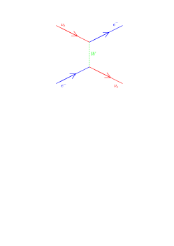
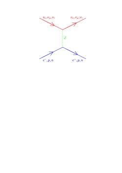
Figure 1: Feynman diagrams of the coherent forward elastic scattering processes that generate the CC potential $V_{\text{CC}}$ through $W$ exchange and the NC potential $V_{\text{NC}}$ through $Z$ exchange.

In the Schrödinger picture the neutrino state with initial flavor $\alpha$ obeys the evolution equation

$$i\,\frac{\text{d}}{\text{d}t}\,|\nu_{\alpha}(p,t)\rangle=\mathcal{H}|\nu_{\alpha}(p,t)\rangle\,,\qquad\text{with}\qquad|\nu_{\alpha}(p,0)\rangle=|\nu_{\alpha}(p)\rangle\,.$$ (3.20)

Let us consider the amplitudes of $\nu_{\alpha}\to\nu_{\beta}$ flavor transitions

$$\psi_{\alpha\beta}(p,t)=\langle\nu_{\beta}(p)|\nu_{\alpha}(p,t)\rangle\,,\qquad\text{with}\qquad\psi_{\alpha\beta}(p,0)=\delta_{\alpha\beta}\,.$$ (3.21)

In other words, $\psi_{\alpha\beta}(p,t)$ is the probability amplitude that a neutrino born at $t=0$ with flavor $\alpha$ is found to have flavor $\beta$ after the time $t$.

From Eqs. (3.16), (3.17) and (3.20), the time evolution equation of the flavor transition amplitudes is

$$i\,\frac{\text{d}}{\text{d}t}\,\psi_{\alpha\beta}(p,t)=\sum_{\rho}\left(\sum_{k}U_{\beta k}\,E_{k}\,U_{\rho k}^{*}+\delta_{\beta\rho}\,V_{\beta}\right)\psi_{\alpha\rho}(p,t)\,.$$ (3.22)

Considering ultrarelativistic neutrinos for which

$$E_{k}\simeq E+\frac{m_{k}^{2}}{2E}\,,\qquad p=E\,,\qquad t=x\,,$$ (3.23)

we have the evolution equation in space

$$i\,\frac{\text{d}}{\text{d}x}\,\psi_{\alpha\beta}(x)=\left(p+\frac{m_{1}^{2}}{2E}+V_{\text{NC}}\right)\psi_{\alpha\beta}(x)+\sum_{\rho}\left(\sum_{k}U_{\beta k}\,\frac{\Delta{m}^{2}_{k1}}{2E}\,U_{\rho k}^{*}+\delta_{\beta e}\,\delta_{\rho e}\,V_{\text{CC}}\right)\psi_{\alpha\rho}(x)\,,$$ (3.24)

where we put in evidence the term $\left(p+m_{1}^{2}/2E+V_{\text{NC}}\right)\psi_{\alpha\beta}(x)$ which generates a phase common to all flavors. This phase is irrelevant for the flavor transitions and can be eliminated by the phase shift

$$\psi_{\alpha\beta}(x)\to\psi_{\alpha\beta}(x)\,e^{-i\left(p+m_{1}^{2}/2E\right)x-i\int_{0}^{x}V_{\text{NC}}(x^{\prime})\,\text{d}x^{\prime}}\,,$$ (3.25)

which does not have any effect on the probability of $\nu_{\alpha}\to\nu_{\beta}$ transitions,

$$P_{\nu_{\alpha}\to\nu_{\beta}}(x)=|\psi_{\alpha\beta}(x)|^{2}\,.$$ (3.26)

Therefore, the relevant evolution equation for the flavor transition amplitudes is

$$i\,\frac{\text{d}}{\text{d}x}\,\psi_{\alpha\beta}(x)=\sum_{\rho}\left(\sum_{k}U_{\beta k}\,\frac{\Delta{m}^{2}_{k1}}{2E}\,U_{\rho k}^{*}+\delta_{\beta e}\,\delta_{\rho e}\,V_{\text{CC}}\right)\psi_{\alpha\rho}(x)\,,$$ (3.27)

which shows that neutrino oscillation in matter, as neutrino oscillation in vacuum, depends on the differences of the squared neutrino masses, not on the absolute value of neutrino masses. Equation (3.27) can be written in matrix form as

$$i\,\frac{\text{d}}{\text{d}x}\,\Psi_{\alpha}=\frac{1}{2E}\left(U\,\Delta{\mathbb{M}}^{2}\,U^{\dagger}+\mathbb{A}\right)\Psi_{\alpha}\,,$$ (3.28)

with, in the case of three-neutrino mixing,

$$\Psi_{\alpha}=\begin{pmatrix}\psi_{\alpha e}\\ \psi_{\alpha\mu}\\ \psi_{\alpha\tau}\end{pmatrix}\,,\qquad\Delta{\mathbb{M}}^{2}=\begin{pmatrix}0&0&0\\ 0&\Delta{m}^{2}_{21}&0\\ 0&0&\Delta{m}^{2}_{31}\end{pmatrix}\,,\qquad\mathbb{A}=\begin{pmatrix}A_{\text{CC}}&0&0\\ 0&0&0\\ 0&0&0\end{pmatrix}\,,$$ (3.29)

where

$$A_{\text{CC}}\equiv 2\,E\,V_{\text{CC}}=2\,\sqrt{2}\,E\,G_{\text{F}}\,N_{e}\,.$$ (3.30)

Since the case of three neutrino mixing is too complicated for an introductory discussion, let us consider the simplest case of two neutrino mixing between $\nu_{e}$, $\nu_{\mu}$ and $\nu_{1}$, $\nu_{2}$. Neglecting an irrelevant common phase, the evolution equation (3.28) can be written as

$$i\frac{\text{d}}{\text{d}x}\begin{pmatrix}\psi_{ee}\\ \psi_{e\mu}\end{pmatrix}=\frac{1}{4E}\begin{pmatrix}-\Delta{m}^{2}\cos{2\vartheta}+2A_{\text{CC}}&\Delta{m}^{2}\sin{2\vartheta}\\ \Delta{m}^{2}\sin{2\vartheta}&\Delta{m}^{2}\cos{2\vartheta}\end{pmatrix}\begin{pmatrix}\psi_{ee}\\ \psi_{e\mu}\end{pmatrix}\,,$$ (3.31)

where $\Delta{m}^{2}\equiv m_{2}^{2}-m_{1}^{2}$ and $\vartheta$ is the mixing angle, such that

$$\nu_{e}=\cos\vartheta\,\nu_{1}+\sin\vartheta\,\nu_{2}\,,\qquad\nu_{\mu}=-\sin\vartheta\,\nu_{1}+\cos\vartheta\,\nu_{2}\,.$$ (3.32)

If the initial neutrino is a $\nu_{e}$, as in solar neutrino experiments, the initial condition for the evolution equation (3.31) is

$$\begin{pmatrix}\psi_{ee}(0)\\ \psi_{e\mu}(0)\end{pmatrix}=\begin{pmatrix}1\\ 0\end{pmatrix}\,,$$ (3.33)

and the probabilities of $\nu_{e}\to\nu_{\mu}$ transitions and $\nu_{e}$ survival are

$$P_{\nu_{e}\to\nu_{\mu}}(x)=|\psi_{e\mu}(x)|^{2}\,,\qquad P_{\nu_{e}\to\nu_{e}}(x)=|\psi_{ee}(x)|^{2}=1-P_{\nu_{e}\to\nu_{\mu}}(x)\,.$$ (3.34)

In practice the evolution equation of the flavor transition amplitudes can always be solved numerically with sufficient degree of precision given enough computational power. Let us discuss the analytical solution of Eq. (3.31) in the case of a matter density profile which is sufficiently smooth. This solution is useful in order to understand the qualitative aspects of the problem.

The effective Hamiltonian matrix in Eq. (3.31) can be diagonalized by the orthogonal transformation

$$\Psi_{e}=U_{\text{M}}\,\Psi\,,\quad\text{with}\quad\Psi_{e}=\begin{pmatrix}\psi_{ee}\\ \psi_{e\mu}\end{pmatrix}\,,\quad U_{\text{M}}=\begin{pmatrix}\cos\vartheta_{\text{M}}&\sin\vartheta_{\text{M}}\\ -\sin\vartheta_{\text{M}}&\cos\vartheta_{\text{M}}\end{pmatrix}\,,\quad\Psi=\begin{pmatrix}\psi_{1}\\ \psi_{2}\end{pmatrix}\,,$$ (3.35)

where $\psi_{k}$ can be thought of as the amplitude of the effective massive neutrino $\nu_{k}$ in matter (although such probability is not measurable, because only flavor neutrinos can be detected). The angle $\vartheta_{\text{M}}$ is the effective mixing angle in matter, given by

$$\tan 2\vartheta_{\text{M}}=\dfrac{\tan 2\vartheta}{1-\dfrac{A_{\text{CC}}}{\Delta{m}^{2}\cos 2\vartheta}}\,.$$ (3.36)

The interesting new phenomenon, discovered by Mikheev and Smirnov in 1985 [89] (and beautifully explained by Bethe in 1986 [90]) is that there is a resonance for

$$A_{\text{CC}}=\Delta{m}^{2}\cos 2\vartheta\,,$$ (3.37)

which corresponds to the electron number density

$$N_{e}^{\text{R}}=\frac{\Delta{m}^{2}\cos 2\vartheta}{2\sqrt{2}EG_{\text{F}}}\,.$$ (3.38)

In the resonance the effective mixing angle is equal to $45^{\circ}$, i.e. the mixing is maximal, leading to the possibility of total transitions between the two flavors if the resonance region is wide enough. This mechanism is called “MSW effect” in honor of Mikheev, Smirnov and Wolfenstein.

The effective squared-mass difference in matter is

$$\Delta{m}^{2}_{\text{M}}=\sqrt{\left(\Delta{m}^{2}\cos 2\vartheta-A_{\text{CC}}\right)^{2}+\left(\Delta{m}^{2}\sin 2\vartheta\right)^{2}}\,.$$ (3.39)

Neglecting an irrelevant common phase, the evolution equation for the amplitudes of the effective massive neutrinos in matter is

$$i\frac{\text{d}}{\text{d}x}\begin{pmatrix}\psi_{1}\\ \psi_{2}\end{pmatrix}=\left[\frac{1}{4E}\begin{pmatrix}-\Delta{m}^{2}_{\text{M}}&0\\ 0&\Delta{m}^{2}_{\text{M}}\end{pmatrix}+\begin{pmatrix}0&-i\text{d}\vartheta_{\text{M}}/\text{d}x\\ i\text{d}\vartheta_{\text{M}}/\text{d}x&0\end{pmatrix}\right]\begin{pmatrix}\psi_{1}\\ \psi_{2}\end{pmatrix}\,,$$ (3.40)

with the initial condition

$$\begin{pmatrix}\psi_{1}(0)\\ \psi_{2}(0)\end{pmatrix}=\begin{pmatrix}\cos\vartheta_{\text{M}}^{0}&-\sin\vartheta_{\text{M}}^{0}\\ \sin\vartheta_{\text{M}}^{0}&\cos\vartheta_{\text{M}}^{0}\end{pmatrix}\begin{pmatrix}1\\ 0\end{pmatrix}=\begin{pmatrix}\cos\vartheta_{\text{M}}^{0}\\ \sin\vartheta_{\text{M}}^{0}\end{pmatrix}\,,$$ (3.41)

where $\vartheta_{\text{M}}^{0}$ is the effective mixing angle in matter at the point of neutrino production.

If the matter density is constant, $\text{d}\vartheta_{\text{M}}/\text{d}x=0$ and the evolutions of the amplitudes of the effective massive neutrinos in matter are decoupled, leading to the transition probability

$$P_{\nu_{e}\to\nu_{\mu}}(x)=\sin^{2}2\vartheta_{\text{M}}\,\sin^{2}\left(\frac{\Delta{m}^{2}_{\text{M}}x}{4E}\right)\,,$$ (3.42)

which has the same structure as the two-neutrino transition probability in vacuum (3.12), with the mixing angle and the squared-mass difference replaced by their effective values in matter.

If the matter density is not constant, it is necessary to take into account the effect of $\text{d}\vartheta_{\text{M}}/\text{d}x$,

$$\dfrac{\text{d}\vartheta_{\text{M}}}{\text{d}x}=\frac{1}{2}\,\frac{\Delta{m}^{2}\sin 2\vartheta}{\left(\Delta{m}^{2}\cos 2\vartheta-A_{\text{CC}}\right)^{2}+\left(\Delta{m}^{2}\sin 2\vartheta\right)^{2}}\,\dfrac{\text{d}A_{\text{CC}}}{\text{d}x}\,,$$ (3.43)

which is maximum at the resonance,

$$\left.\dfrac{\text{d}\vartheta_{\text{M}}}{\text{d}x}\right|_{\text{R}}=\frac{1}{2\,\tan 2\vartheta}\left.\dfrac{\text{d}\ln N_{e}}{\text{d}x}\right|_{\text{R}}\,.$$ (3.44)

This is illustrated in the left panel of Fig. 2 for $\Delta{m}^{2}=7\times 10^{-6}\,\text{eV}^{2}$, $\sin^{2}2\vartheta=10^{-3}$. One can see that for $N_{e}\ll N_{e}^{\text{R}}$ the effective mixing angle is practically equal to the mixing angle in vacuum, $\vartheta_{\text{M}}\simeq\vartheta$, for $N_{e}\simeq N_{e}^{\text{R}}$ the effective mixing angle varies very rapidly with the electron number density, passing through $45^{\circ}$ at $N_{e}=N_{e}^{\text{R}}$ and going rapidly to $90^{\circ}$ for $N_{e}>N_{e}^{\text{R}}$.

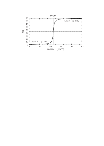
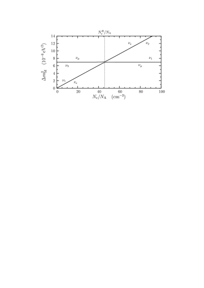
Figure 2: Effective mixing angle $\vartheta_{\text{M}}$ (left) and effective squared-mass difference $\Delta{m}^{2}_{\text{M}}$ (right) in matter as functions of the electron number density $N_{e}$ divided by the Avogadro number $N_{\text{A}}$, for $\Delta{m}^{2}=7\times 10^{-6}\,\text{eV}^{2}$, $\sin^{2}2\vartheta=10^{-3}$. $N_{e}^{\text{R}}\equiv\Delta{m}^{2}\cos 2\vartheta/2\sqrt{2}EG_{\text{F}}$ is the electron number density at the resonance, where $\vartheta_{\text{M}}=45^{\circ}$.

The right panel of Fig. 2 shows the corresponding behavior of the effective squared-mass difference $\Delta{m}^{2}_{\text{M}}$, which is useful in order to understand how the presence of a resonance can induce an almost complete $\nu_{e}\to\nu_{\mu}$ conversion of solar neutrinos. If the mixing parameters are such that at the center of the sun $N_{e}\gg N_{e}^{\text{R}}$, the effective mixing angle is practically $90^{\circ}$ and electron neutrinos are produced as almost pure $\nu_{2}$. As the neutrino propagates out of the sun, it crosses the resonance at $N_{e}=N_{e}^{\text{R}}$, where the energy gap between $\nu_{1}$ and $\nu_{2}$ is minimum. If the resonance is crossed adiabatically, the neutrino remains $\nu_{2}$ and exits the sun as $\nu_{2}=\sin\vartheta\,\nu_{e}+\cos\vartheta\,\nu_{\mu}$, which is almost equal to $\nu_{\mu}$ if the mixing angle is small, leading to almost complete $\nu_{e}\to\nu_{\mu}$ conversion. This is the case in which the MSW effect is most effective and striking, since a large conversion is achieved in spite of a small mixing angle.

If the resonance is not crossed adiabatically, $\nu_{2}\to\nu_{1}$ transitions occur in an interval around the resonance and the neutrino emerges out of the sun as a mixture of $\nu_{2}$ and $\nu_{1}$, leading to partial conversion of $\nu_{e}$ into $\nu_{\mu}$. Quantitatively, we can write the amplitudes of $\nu_{1}$ and $\nu_{2}$ at any point $x$ after resonance crossing as

$$\psi_{1}(x)=\hbox{} \hbox{}\left[\cos\vartheta_{\text{M}}^{0}\exp\left(i\int_{0}^{x_{\text{R}}}\frac{\Delta{m}^{2}_{\text{M}}(x^{\prime})}{4E}\,\text{d}x^{\prime}\right)\mathcal{A}_{11}^{\text{R}}+\sin\vartheta_{\text{M}}^{0}\exp\left(-i\int_{0}^{x_{\text{R}}}\frac{\Delta{m}^{2}_{\text{M}}(x^{\prime})}{4E}\,\text{d}x^{\prime}\right)\mathcal{A}_{21}^{\text{R}}\right]$$

$$\hbox{}\times\exp\left(i\int_{x_{\text{R}}}^{x}\frac{\Delta{m}^{2}_{\text{M}}(x^{\prime})}{4E}\,\text{d}x^{\prime}\right)\,,$$ (3.45)

$$\psi_{2}(x)=\hbox{} \hbox{}\left[\cos\vartheta_{\text{M}}^{0}\exp\left(i\int_{0}^{x_{\text{R}}}\frac{\Delta{m}^{2}_{\text{M}}(x^{\prime})}{4E}\,\text{d}x^{\prime}\right)\mathcal{A}_{12}^{\text{R}}+\sin\vartheta_{\text{M}}^{0}\exp\left(-i\int_{0}^{x_{\text{R}}}\frac{\Delta{m}^{2}_{\text{M}}(x^{\prime})}{4E}\,\text{d}x^{\prime}\right)\mathcal{A}_{22}^{\text{R}}\right]$$

$$\hbox{}\times\exp\left(-i\int_{x_{\text{R}}}^{x}\frac{\Delta{m}^{2}_{\text{M}}(x^{\prime})}{4E}\,\text{d}x^{\prime}\right)\,,$$ (3.46)

where $\mathcal{A}_{kj}^{\text{R}}$ is the amplitude of $\nu_{k}\to\nu_{j}$ transitions in the resonance.

Considering $x$ as the detection point on the earth, practically in vacuum, the probability of $\nu_{e}$ survival is given by

$$\overline{P}_{\nu_{e}\to\nu_{e}}(x)=|\psi_{ee}(x)|^{2}\,,\qquad\text{with}\qquad\psi_{ee}(x)=\cos\vartheta\,\psi_{1}(x)+\sin\vartheta\,\psi_{2}(x)\,.$$ (3.47)

If $\Delta{m}^{2}\gg 10^{-10}\,\text{eV}^{2}$ all the phases in Eqs. (3.45) and (3.46) are very large and rapidly oscillating as functions of the neutrino energy. In this case, the average of the transition probability over the energy resolution of the detector washes out all interference terms and only the averaged survival probability

$$\overline{P}_{\nu_{e}\to\nu_{e}}^{\,\text{sun}}=\hbox{} \hbox{}\cos^{2}\vartheta\,\cos^{2}\vartheta_{\text{M}}^{0}\,|\mathcal{A}_{11}^{\text{R}}|^{2}+\cos^{2}\vartheta\,\sin^{2}\vartheta_{\text{M}}^{0}\,|\mathcal{A}_{21}^{\text{R}}|^{2}$$

$$\hbox{}+\sin^{2}\vartheta\,\cos^{2}\vartheta_{\text{M}}^{0}\,|\mathcal{A}_{12}^{\text{R}}|^{2}+\sin^{2}\vartheta\,\sin^{2}\vartheta_{\text{M}}^{0}\,|\mathcal{A}_{22}^{\text{R}}|^{2}\,,$$ (3.48)

which is independent from the sun–earth distance, is measurable. Taking into account that conservation of probability implies that

$$|\mathcal{A}_{11}^{\text{R}}|^{2}=|\mathcal{A}_{22}^{\text{R}}|^{2}=1-P_{\text{c}}\,,\qquad|\mathcal{A}_{12}^{\text{R}}|^{2}=|\mathcal{A}_{21}^{\text{R}}|^{2}=P_{\text{c}}\,,$$ (3.49)

where $P_{\text{c}}$ is the $\nu_{1}\leftrightarrows\nu_{2}$ crossing probability at the resonance, we obtain the so-called Parke formula [91] for the averaged $\nu_{e}$ survival probability:

$$\overline{P}_{\nu_{e}\to\nu_{e}}^{\,\text{sun}}=\frac{1}{2}+\left(\frac{1}{2}-P_{\text{c}}\right)\cos 2\vartheta_{\text{M}}^{0}\,\cos 2\vartheta\,.$$ (3.50)

This formula has been widely used for the analysis of solar neutrino data.

The main problem in the application of the Parke formula (3.50) is the calculation of the crossing probability. This probability must involve the energy gap $\Delta{m}^{2}_{\text{M}}/2E$ between $\nu_{1}$ and $\nu_{2}$ and the off diagonal terms proportional to $\text{d}\vartheta_{\text{M}}/\text{d}x$ in Eq. (3.40), which cause the $\nu_{1}\leftrightarrows\nu_{2}$ transitions. Indeed, the crossing probability can be written as [92, 93, 94, 95]

$$P_{\text{c}}=\frac{\exp\left(-\frac{\pi}{2}\gamma F\right)-\exp\left(-\frac{\pi}{2}\gamma\frac{F}{\sin^{2}\vartheta}\right)}{1-\exp\left(-\frac{\pi}{2}\gamma\frac{F}{\sin^{2}\vartheta}\right)}\,,$$ (3.51)

where $\gamma$ is the adiabaticity parameter

$$\gamma=\left.\frac{\Delta{m}^{2}_{\text{M}}/2E}{2|\text{d}\vartheta_{\text{M}}/\text{d}x|}\right|_{\text{R}}=\frac{\Delta{m}^{2}\sin^{2}2\vartheta}{2E\cos 2\vartheta\left|\text{d}\ln N_{e}/\text{d}x\right|_{\text{R}}}\,.$$ (3.52)

If $\gamma$ is large, the resonance is crossed adiabatically and $P_{\text{c}}\ll 1$, leading to

$$\overline{P}_{\nu_{e}\to\nu_{e}}^{\,\text{sun, adiabatic}}=\frac{1}{2}+\frac{1}{2}\,\cos 2\vartheta_{\text{M}}^{0}\,\cos 2\vartheta\,.$$ (3.53)

The parameter $F$ in Eq. (3.51) depends on the electron density profile. The left panel in Figure 3 shows the Standard Solar Model (SSM) electron density profile in the sun [96], which is well approximated by the exponential

$$N_{e}(R)=N_{e}(0)\exp\left(-\frac{R}{R_{0}}\right)\,,\quad\text{with}\quad N_{e}(0)=245\,N_{\text{A}}/\text{cm}^{3}\,,\quad\text{and}\quad R_{0}=\frac{R_{\odot}}{10.54}\,,$$ (3.54)

where $R$ is the distance from the center of the sun and $R_{\odot}$ is the solar radius. For an exponential electron density profile the parameter $F$ is given by [92, 93, 94, 97, 98, 99]

$$F=1-\tan^{2}\vartheta\,.$$ (3.55)

For $\left|\text{d}\ln N_{e}/\text{d}x\right|_{\text{R}}$ the authors of Ref. [100] suggested the practical prescription, verified with numerical solutions of the differential evolution equation, to calculate it numerically from the SSM electron density profile for $R\leq 0.904R_{\odot}$ and take the constant value $18.9/R_{\odot}$ for $R>0.904R_{\odot}$, where the exponential approximation (3.54) breaks down.

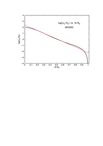
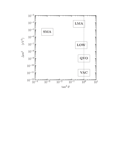
Figure 3: Left: Standard Solar Model electron density profile in the sun as a function of the ratio $R/R_{\odot}$ [96]. The straight line represents the approximation in Eq. (3.54). Right: The conventional names for regions in the $\tan^{2}\vartheta$–$\Delta{m}^{2}$ plane obtained from the analysis of solar neutrino data. The vertical dotted line correspond to maximal mixing.

For the analysis of solar neutrino data it is also necessary to take into account the matter effect along the propagation of neutrinos in the earth during the night (the so-called “$\nu_{e}$ regeneration in the earth”), which can generate a day-night asymmetry of the rates. The probability of solar $\nu_{e}$ survival after crossing the earth is given by [18, 101]

$$P_{\nu_{e}\to\nu_{e}}^{\,\text{sun+earth}}=\overline{P}_{\nu_{e}\to\nu_{e}}^{\,\text{sun}}+\frac{\left(1-2\overline{P}_{\nu_{e}\to\nu_{e}}^{\,\text{sun}}\right)\left(P_{\nu_{2}\to\nu_{e}}^{\,\text{earth}}-\sin^{2}\vartheta\right)}{\cos\!2\vartheta}\,.$$ (3.56)

Since the earth density profile is not a smooth function, the probability $P_{\nu_{2}\to\nu_{e}}^{\,\text{earth}}$ must be calculated numerically. A good approximation is obtained by approximating the earth density profile with a step function (see Refs. [102, 103, 104, 105, 106]). According to Eq. (3.40), the effective massive neutrinos propagate as plane waves in regions of constant density, with a phase $\exp\left(\pm i\Delta{m}^{2}_{\text{M}}\Delta{x}/4E\right)$, where $\Delta{x}$ is the width of the step. At the boundaries of steps the wave functions of flavor neutrinos are joined, according to the scheme

$$\Psi(x_{n})=\hbox{} \hbox{}\left[U_{\text{M}}\,\Phi(x_{n}-x_{n-1})\,U_{\text{M}}^{\dagger}\right]_{(n)}\left[U_{\text{M}}\,\Phi(x_{n-1}-x_{n-2})\,U_{\text{M}}^{\dagger}\right]_{(n-1)}$$

$$\hbox{}\ldots\left[U_{\text{M}}\,\Phi(x_{2}-x_{1})\,U_{\text{M}}^{\dagger}\right]_{(2)}\left[U_{\text{M}}\,\Phi(x_{1}-x_{0})\,U_{\text{M}}^{\dagger}\right]_{(1)}U\,\Psi(x_{0})\,.$$ (3.57)

where $x_{0}$ is the coordinate of the point in which the neutrino enters the earth, $x_{1}$, $x_{2}$, …, $x_{n}$ are the boundaries of $n$ steps with which the earth density profile is approximated, $\Phi(\Delta{x})=\text{diag}\!\left(\exp\left(-i\Delta{m}^{2}_{\text{M}}\Delta{x}/4E\right)\,,\,\exp\left(i\Delta{m}^{2}_{\text{M}}\Delta{x}/4E\right)\right)$, and the notation $\left[\ldots\right]_{(i)}$ indicates that all the matter-dependent quantities in the square brackets must be evaluated with the matter density in the $i^{\text{th}}$ step, that extends from $x_{i-1}$ to $x_{i}$.

The right panel in Fig. 3 shows the conventional names for regions in the $\tan^{2}\vartheta$–$\Delta{m}^{2}$ plane obtained from the analysis of solar neutrino data. The Small Mixing Angle (SMA) region is the one where the mixing angle is very small and the resonant enhancement of flavor transitions due to the MSW effect is more efficient. However, as explained in Section 4.1 there is currently a very strong evidence in favor of the Large Mixing Angle (LMA) region, in which both the mixing angle and $\Delta{m}^{2}$ are large. Other regions with large mixing are: the low $\Delta{m}^{2}$ (LOW) region, the Quasi-Vacuum-Oscillations (QVO) region, and the VACuum Oscillations region (VAC). In the SMA, LMA and LOW regions vacuum oscillations due to the sun–earth distance are not observable because the $\Delta{m}^{2}$ is too high and interference effects are washed out by the average over the energy resolution of the detector (in these cases the Parke formula (3.50) applies). In the QVO region both matter effects and vacuum oscillations are important [107, 108, 109, 100]. In the VAC region matter effects are negligible and vacuum oscillations are dominant.

Concluding this Section on the theory of neutrino oscillations, let us mention that the evolution equation (3.28) allows to prove easily that the Majorana phases in the mixing matrix do not have any effect on neutrino oscillations in vacuum [110, 111] as well as in matter [112], because the diagonal matrix of Majorana phases $D(\lambda_{21},\lambda_{31})$ on the right of the mixing matrix in Eq. (2.48) cancels in the product $U\Delta{\mathbb{M}}^{2}U^{\dagger}$. Therefore, the Dirac or Majorana nature of neutrinos cannot be distinguished in neutrino oscillations.

4 Neutrino oscillation experiments

In this Section we review the main results of the oscillation experiments which are connected with the existing model-independent evidences in favor of oscillations of solar and atmospheric neutrinos and the interpretation of the experimental data in the framework of three neutrino mixing, discussed in Section 5. We do not discuss the results of several short-baseline neutrino (SBL) oscillation experiments, which have probed scales of $\Delta{m}^{2}$ bigger than about $0.1\,\text{eV}^{2}$, that are larger than the scales of $\Delta{m}^{2}$ indicated by solar and atmospheric neutrino data. The SBL experiments whose data give the most stringent constraints on the different oscillation channels are listed in Table 1.

Experiment	Channels
Bugey	$\bar{\nu}_{e}\to\bar{\nu}_{e}$ [64]
CDHS	$\overset{\scriptscriptstyle(-)}{\nu}_{\mu}\to\overset{\scriptscriptstyle(-)}{\nu}_{\mu}$ [71]
CCFR	$\overset{\scriptscriptstyle(-)}{\nu}_{\mu}\to\overset{\scriptscriptstyle(-)}{\nu}_{\mu}$ [113], $\overset{\scriptscriptstyle(-)}{\nu}_{\mu}\to\overset{\scriptscriptstyle(-)}{\nu}_{e}$ [72], $\overset{\scriptscriptstyle(-)}{\nu}_{e}\to\overset{\scriptscriptstyle(-)}{\nu}_{\tau}$ [72] $\overset{\scriptscriptstyle(-)}{\nu}_{e}\to\overset{\scriptscriptstyle(-)}{\nu}_{e}$ [72]
LSND	$\bar{\nu}_{\mu}\to\bar{\nu}_{e}$ [75], $\nu_{\mu}\to\nu_{e}$ [114],
KARMEN	$\bar{\nu}_{\mu}\to\bar{\nu}_{e}$ [76]
NOMAD	$\nu_{\mu}\to\nu_{e}$ [74] $\nu_{\mu}\to\nu_{\tau}$ [115], $\nu_{e}\to\nu_{\tau}$ [115]
CHORUS	$\nu_{\mu}\to\nu_{\tau}$ [73], $\nu_{e}\to\nu_{\tau}$ [73]
NuTeV	$\overset{\scriptscriptstyle(-)}{\nu}_{\mu}\to\overset{\scriptscriptstyle(-)}{\nu}_{e}$ [116]

Table 1: Short-baseline experiments (SBL) whose data give the most stringent constraints on different oscillation channels.

All the SBL experiments in Table 1 did not observe any indication of neutrino oscillations, except the LSND experiment [114, 75]. A large part of the region in the $\sin^{2}2\vartheta$–$\Delta{m}^{2}$ plane allowed by LSND has been excluded by the results of other experiments which are sensitive to similar values of the neutrino oscillation parameters (KARMEN [76], CCFR [117], NOMAD [74]; see Ref. [118] for an accurate combined analysis of LSND and KARMEN data). The MiniBooNE experiment [119] running at Fermilab will tell us the validity of the LSND indication in the near future.

Some years ago the oscillations indicated by the LSND experiment could be accommodated together with solar and atmospheric neutrino oscillations in the framework of four-neutrino mixing, in which there are three light active neutrinos and one light sterile neutrino (see Refs. [21, 120, 121, 122] and references in Ref. [39]). However, the global fit of recent data in terms of four-neutrino mixing is not good [123], disfavoring such possibility. Therefore, in this review we discuss only three-neutrino mixing, which cannot explain the LSND indication, awaiting the response of MiniBooNE before engaging in wild speculations (see Refs. [124, 125, 126, 127, 128, 129, 130, 131]).

4.1 Solar neutrino experiments and KamLAND

At the end of the 60’s the radiochemical Homestake experiment [9] began the observation of solar neutrinos through the charged-current reaction [132, 133]

$$\nu_{e}+{}^{37}\text{Cl}\to{}^{37}\text{Ar}+e^{-}\,,$$ (4.1)

with a threshold $E_{\text{th}}^{\text{Cl}}=0.814\,\text{MeV}$ which allows to observe mainly ${}^{7}\text{Be}$ and ${}^{8}\text{B}$ neutrinos produced, respectively, in the reactions $e^{-}+{}^{7}\text{Be}\to{}^{7}\text{Li}+\nu_{e}\,(E=0.8631\,\text{MeV})$ and ${}^{8}\text{B}\to{}^{8}\text{Be}^{*}+e^{+}+\nu_{e}\,(E\lesssim 15\,\text{MeV})$ of the thermonuclear $pp$ cycle that produces energy in the core of the sun (see Refs. [134, 15]).

The Homestake experiment is called “radiochemical” because the ${}^{37}\text{Ar}$ atoms were extracted every $\sim$35 days from the detector tank containing 615 tons of tetrachloroethylene ($\text{C}_{2}\text{Cl}_{4}$) through chemical methods and counted in small proportional counters which detect the Auger electron produced in the electron-capture of ${}^{37}\text{Ar}$. As all solar neutrino detectors, the Homestake tank was located deep underground (1478 m) in order to have a good shielding from cosmic ray muons. The Homestake experiment detected solar electron neutrinos for about 30 years [9], measuring a flux which is about one third of the one predicted Standard Solar Model (SSM) [96]:

$$\frac{\Phi_{\text{Cl}}^{\text{Hom}}}{\Phi_{\text{Cl}}^{\text{SSM}}}=0.34\pm 0.03\,.$$ (4.2)

This deficit was called “the solar neutrino problem”.

The solar neutrino problem was confirmed in the late 80’s by the real-time water Cherenkov Kamiokande experiment [85] (3000 tons of water, 1000 m underground) which observed solar neutrinos through the elastic scattering (ES) reaction

$$\nu+e^{-}\to\nu+e^{-}\,,$$ (4.3)

which is mainly sensitive to electron neutrinos, whose cross section is about six time larger than the cross section of muon and tau neutrinos. The experiment is called “real-time” because the Cherenkov light produced in water by the recoil electron in the reaction (4.3) is observed in real time. The solar neutrino signal is separated statistically from the background using the fact that the recoil electron preserves the directionality of the incoming neutrino. The energy threshold of the Kamiokande experiment was 6.75 MeV, allowing only the detection of ${}^{8}\text{B}$ neutrinos. After 1995 the Kamiokande experiment has been replaced by the bigger Super-Kamiokande experiment [8, 66, 67] (50 ktons of water, 1000 m underground) which has measured with high accuracy the flux of solar ${}^{8}\text{B}$ neutrinos with an energy threshold of 4.75 MeV, obtaining [66]

$$\frac{\Phi_{\text{ES}}^{\text{S-K}}}{\Phi_{\text{ES}}^{\text{SSM}}}=0.465\pm 0.015\,.$$ (4.4)

In the early 90’s the GALLEX [61] (30.3 tons of ${}^{71}\text{Ga}$, 1400 m underground) and SAGE [62] (50 tons of ${}^{71}\text{Ga}$, 2000 m underground) radiochemical experiments started the observation of solar electron neutrinos through the charged-current reaction [135]

$$\nu_{e}+{}^{71}\text{Ga}\to{}^{71}\text{Ge}+e^{-}\,,$$ (4.5)

which has the low energy threshold of 0.233 MeV, that allows the detection of the so-called $pp$ neutrinos produced in the main reaction $p+p\to d+e^{+}+\nu_{e}\,(E\lesssim 0.42\,\text{MeV})$ of the $pp$ cycle, besides the ${}^{7}\text{Be}$, ${}^{8}\text{B}$ and other neutrinos. After 1997 the GALLEX experiment has been upgraded, changing its name to GNO [63]. The combined results of the three Gallium experiments confirm the solar neutrino problem:

$$\frac{\Phi_{\text{Ga}}}{\Phi_{\text{Ga}}^{\text{SSM}}}=0.56\pm 0.03\,.$$ (4.6)

Although it was difficult to doubt of the Standard Solar Model, which was well tested by helioseismological measurements (see Ref. [136]), and it was difficult to explain the different suppression of solar $\nu_{e}$’s observed in different experiments with astrophysical mechanisms, a definitive model-independent proof that the solar neutrino problem is due to neutrino physics was lacking until the real-time heavy-water Cherenkov detector SNO [7, 10, 11] (1 kton of $\text{D}_{2}\text{O}$, 2073 m underground) observed solar ${}^{8}\text{B}$ neutrinos through the charged-current (CC) reaction

$$\nu_{e}+d\to p+p+e^{-}\,,$$ (4.7)

with $E_{\text{th,CC}}^{\text{SNO}}=8.2\,\text{MeV}$ and the neutral-current (NC) reaction

$$\nu+d\to p+n+\nu\,,$$ (4.8)

with $E_{\text{th,NC}}^{\text{SNO}}=2.2\,\text{MeV}$, besides the ES reaction (4.3) with $E_{\text{th,ES}}^{\text{SNO}}=7.0\,\text{MeV}$. The observation of solar neutrinos through the CC and NC reactions has provided the breakthrough for the definitive solution of the solar neutrino problem in favor of new neutrino physics. The charged-current reaction is very important because it allows to measure with high statistics the energy spectrum of solar $\nu_{e}$’s. The neutral current reaction is extremely important for the measurement of the total flux of active $\nu_{e}$, $\nu_{\mu}$ and $\nu_{\tau}$, which interact with the same cross section.

In June 2001 the combination of the first SNO CC data [7] and the high-precision Super-Kamiokande ES data [8] allowed to extract a model-independent indication of the oscillations of solar electron neutrinos into active $\nu_{\mu}$’s and/or $\nu_{\tau}$’s [7] (see also Refs. [137, 138]). In April 2002 the observation of solar neutrinos through the NC and CC reactions allowed the SNO experiment [10] to solve definitively the long-standing solar neutrino problem in favor of the existence of $\nu_{e}\to\nu_{\mu},\nu_{\tau}$ transitions. In this first phase [10], called “$\text{D}_{2}\text{O}$ phase”, the neutron produced in the neutral-current reaction (4.8) was detected by observing the photon produced in the reaction

$$n+d\to{}^{3}\text{H}+\gamma\,(E_{\gamma}=6.25\,\text{MeV})\,.$$ (4.9)

In September 2003 the SNO collaboration released the data obtained in the second phase [11], called “salt phase”, in which 2 tons of salt has been added to the heavy water in the SNO detector, allowing the detection of the neutron produced in the neutral-current reaction (4.8) by observing the photons produced in the reaction

$$n+{}^{35}\text{Cl}\to{}^{36}\text{Cl}+\text{several $\gamma$'s}\,(E_{\gamma}^{\text{tot}}=8.6\,\text{MeV})\,.$$ (4.10)

The better signature given by several photons and the higher cross-section of reaction (4.10) with respect to reaction (4.9) have allowed the SNO collaboration to measure with good precision the total flux of active neutrinos coming from ${}^{8}\text{B}$ decay in the core of the sun [11]:

$$\Phi_{\text{NC}}^{\text{SNO}}=5.21\pm 0.47\times 10^{6}\,\text{cm}^{-2}\,\text{s}^{-1}\,,$$ (4.11)

which is in good agreement with the value predicted by the Standard Solar Model (SSM) [96],

$$\Phi_{{}^{8}\text{B}}^{\text{SSM}}=5.05\,{}^{+1.01}_{-0.81}\times 10^{6}\,\text{cm}^{-2}\,\text{s}^{-1}\,.$$ (4.12)

On the other hand, the flux of electron neutrinos coming from ${}^{8}\text{B}$ decay measured through the CC reaction (4.7) is only [11]

$$\Phi_{\text{CC}}^{\text{SNO}}=1.59{}^{+0.10}_{-0.11}\times 10^{6}\,\text{cm}^{-2}\,\text{s}^{-1}\,.$$ (4.13)

The fact that the ratio [11]

$$\frac{\Phi_{\text{CC}}^{\text{SNO}}}{\Phi_{\text{NC}}^{\text{SNO}}}=0.306\pm 0.035$$ (4.14)

differs from unity by about 19 standard deviations is a very convincing proof that solar electron neutrinos have transformed into muon and/or tau neutrinos on their way to the earth.

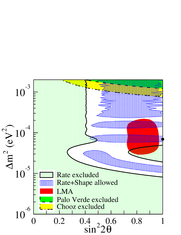
Figure 4: Left: Allowed regions of neutrino oscillation parameters obtained from the global analysis of solar neutrino data [11]. The best-fit point is marked by a star. Right: KamLAND excluded regions of neutrino oscillation parameters for the rate analysis and allowed regions for the combined rate and energy spectrum analysis at 95% C.L [12]. At the top are the 95% C.L. excluded region from CHOOZ [139] and Palo Verde [78] experiments, respectively. The dark area is the 95% C.L. LMA allowed region obtained in Ref. [140]. The thick dot indicates the best fit of KamLAND data.

The result of the global analysis of all solar neutrino data in terms of the simplest hypothesis of two-neutrino oscillations favors the so-called Large Mixing Angle (LMA) region with effective two-neutrino mixing parameters $\Delta{m}^{2}_{\text{SUN}}\sim 7\times 10^{-5}\,\text{eV}^{2}$ and $\tan^{2}\vartheta_{\text{SUN}}\sim 0.4$, as shown in the left panel in Fig. 4, taken from Ref. [11].

A spectacular proof of the correctness of the LMA region has been obtained at the end of 2002 in the KamLAND long-baseline $\bar{\nu}_{e}$ disappearance experiment [12], in which the suppression

$$\frac{N^{\text{KamLAND}}_{\text{observed}}}{N^{\text{KamLAND}}_{\text{expected}}}=0.611\pm 0.094\,.$$ (4.15)

of the $\bar{\nu}_{e}$ flux produced by nuclear reactors at an average distance of about 180 km was observed. The right panel in Fig. 4 shows the regions of oscillation parameters allowed by KamLAND, compared with the allowed LMA region obtained in Ref. [140] in 2002 after the release of the data of the first $\text{D}_{2}\text{O}$ phase of the SNO experiment [10]. From the right panel in Fig. 4 one can see that the LMA region and the KamLAND allowed regions overlap in two subregions at $\Delta{m}^{2}_{\text{SUN}}\simeq 7\times 10^{-5}\,\text{eV}^{2}$ and $\Delta{m}^{2}_{\text{SUN}}\simeq 1.5\times 10^{-4}\,\text{eV}^{2}$. Therefore, the combined fit of 2002 solar neutrino data and KamLAND data yielded two allowed LMA subregions. The 2003 SNO salt phase data lead to a restriction of the LMA region allowed by solar neutrino data, which favors the lower LMA subregion, as shown in the left panel in Fig. 5 which depicts the most updated allowed region of the two-neutrino oscillation parameters obtained from the global analysis of solar and KamLAND neutrino data. The effective two-neutrino mixing parameters are constrained at 99.73% C.L. ($3\sigma$) in the ranges [141]

$$5.4\times 10^{-5}\,\text{eV}^{2}<\Delta{m}^{2}_{\text{SUN}}<9.4\times 10^{-5}\,\text{eV}^{2}\,,$$ (4.16)

$$0.30<\tan^{2}\vartheta_{\text{SUN}}<0.64\,,$$ (4.17)

with best-fit values [141]

$$\Delta{m}^{2\,\text{bf}}_{\text{SUN}}=6.9\times 10^{-5}\,\text{eV}^{2}\,,\qquad\tan^{2}\vartheta_{\text{SUN}}^{\text{bf}}=0.43\,.$$ (4.18)

Maximal mixing is excluded at a confidence level equivalent to $5.4\sigma$ [11].

Transitions of solar $\nu_{e}$’s into sterile states are disfavored by the data. The right panel in Fig. 5 shows the allowed regions in the $\text{f}_{\text{B,total}}$–$\sin^{2}\eta$ plane obtained in Ref. [142] before the release of the SNO salt data, where $\text{f}_{\text{B,total}}=\Phi_{{}^{8}\text{B}}/\Phi_{{}^{8}\text{B}}^{\text{SSM}}$ is the ratio of the ${}^{8}\text{B}$ solar neutrino flux and its value predicted by the Standard Solar Model (SSM) [96]. The parameter $\sin^{2}\eta$ quantifies the fraction of solar $\nu_{e}$’s that transform into sterile $\nu_{s}$: $\nu_{e}\to\cos\eta\,\nu_{a}+\sin\eta\,\nu_{s}$, where $\nu_{a}$ are active neutrinos. From the right panel of Fig. 5 it is clear that there is a correlation between $\text{f}_{\text{B,total}}$ and $\sin^{2}\eta$, which is due to the constraint on the total flux of ${}^{8}\text{B}$ active neutrinos given by the SNO neutral-current measurement: disappearance into sterile states is possible only if the ${}^{8}\text{B}$ solar neutrino flux is larger than the SSM prediction. The allowed ranges for $\Phi_{{}^{8}\text{B}}$ and $\sin^{2}\eta$ are [142]

$$\Phi_{{}^{8}\text{B}}=1.00\pm 0.06\,\Phi_{{}^{8}\text{B}}^{\text{SSM}}\,,\quad\sin^{2}\eta<0.52\,.$$ (4.19)

The allowed interval for $\Phi_{{}^{8}\text{B}}$ shows a remarkable agreement of the data with the SSM, independently from possible $\nu_{e}\to\nu_{s}$ transitions. The recent SNO salt data do not allow to improve significantly the bound on $\sin^{2}\eta$ [143].

In the future it is expected that the KamLAND experiment will allow to reach a relatively high accuracy in the determination of $\Delta{m}^{2}_{\text{SUN}}$ [144], whereas new low-energy solar neutrino experiments or a new dedicated reactor neutrino experiment are needed in order to improve significantly our knowledge of the solar effective mixing angle $\vartheta_{\text{SUN}}$ [145, 146, 147].

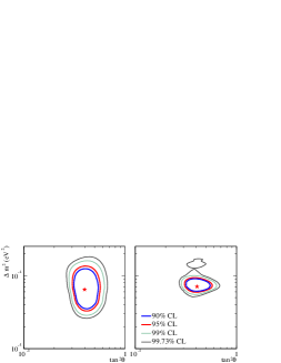
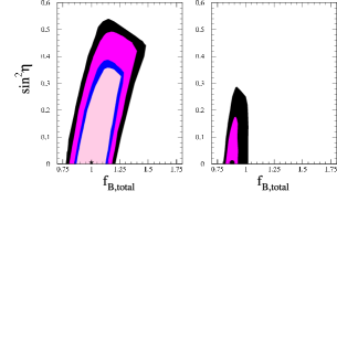
Figure 5: Left: Allowed regions obtained from the global analysis of solar and KamLAND data [11]. Right: Allowed 90%, 95%, 99%, 99.73% C.L. regions obtained from the global analysis of solar and KamLAND data [142]. The best-fit points are marked by stars.

4.2 Atmospheric neutrino experiments and K2K

Atmospheric neutrinos are produced by cosmic rays (mainly protons) which interact with the atmosphere producing pions, which decay into muon and neutrinos,

$$\pi^{+}\to\mu^{+}+\nu_{\mu}\,,\qquad\pi^{-}\to\mu^{-}+\bar{\nu}_{\mu}\,.$$ (4.20)

At low energy the muons decay before hitting the ground into electrons and neutrinos,

$$\mu^{+}\to e^{+}+\nu_{e}+\bar{\nu}_{\mu}\,,\qquad\mu^{-}\to e^{-}+\bar{\nu}_{e}+\nu_{\mu}\,.$$ (4.21)

Hence, the predicted ratio of $\nu_{\mu}+\bar{\nu}_{\mu}$ and $\nu_{e}+\bar{\nu}_{e}$ is about 2 at neutrino energy $E\lesssim 1\text{GeV}$. At higher energies the ratio increases, but it can be calculated with reasonable accuracy (about 5%). On the other hand, the calculation of the absolute value of the atmospheric neutrino flux suffers from a large uncertainty (20% or 30%) due to the uncertainty of the absolute value of the cosmic ray flux and the uncertainties of the cross sections of cosmic ray interactions with the nuclei in the atmosphere (see Ref. [28]). Therefore, the traditional way that has been followed for testing the atmospheric neutrino flux calculation is to measure the ratio of ratios

$$R\equiv\frac{\left[N(\nu_{\mu}+\bar{\nu}_{\mu})/N(\nu_{e}+\bar{\nu}_{e})\right]_{\text{data}}}{\left[N(\nu_{\mu}+\bar{\nu}_{\mu})/N(\nu_{e}+\bar{\nu}_{e})\right]_{\text{theo}}}\,,$$ (4.22)

where the subscripts “data” and “theo” indicate, respectively, the measured and calculated ratio. If nothing happens to neutrinos on their way to the detector the ratio of ratios should be equal to one.

Atmospheric neutrinos are observed through high-energy charged-current interactions in which the flavor, direction and energy of the neutrino are strongly correlated with the measured flavor, direction and energy of the produced charged lepton.

In 1988 the Kamiokande [4] and IMB [5] experiments measured a ratio of ratios significantly lower than one. The current values of $R$ measured in the Super-Kamiokande experiment are [148]

$$R^{\text{S-K}}(E<1.33\,\text{GeV})=0.638\pm 0.053\,,$$ (4.23)

$$R^{\text{S-K}}(E>1.33\,\text{GeV})=0.675\pm 0.087\,.$$ (4.24)

The boundary of 1.33 GeV has been chosen by the Super-Kamiokande Collaboration for historical reasons connected with proton decay search.

Also the Soudan-2 experiment [83] observed a ratio of ratios significantly lower than one,

$$R^{\text{Soudan-2}}=0.69\pm 0.12\,,$$ (4.25)

and the MACRO experiment [84] measured a disappearance of upward-going muons.

Although the values (4.23), (4.24) and (4.25) of the ratio of ratios suggest an evidence of an atmospheric neutrino anomaly probably due to neutrino oscillations, they are not completely model-independent.

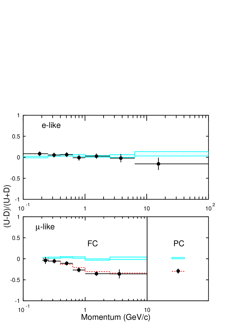
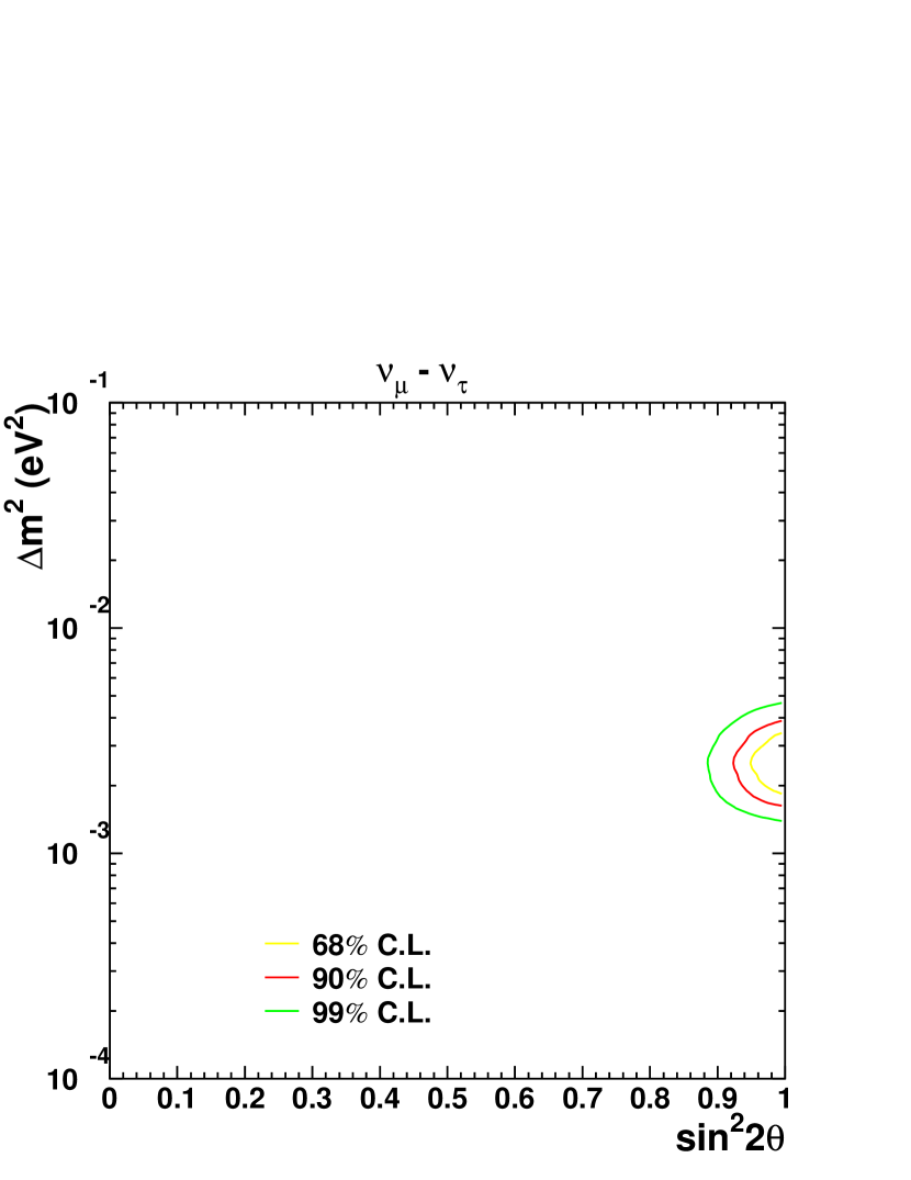
Figure 6: Left: Up-down Super-Kamiokande asymmetry as a function of momentum for $e$-like and $\mu$-like events generated, respectively, by atmospheric $\nu_{e}$, $\bar{\nu}_{e}$ and $\nu_{\mu}$, $\bar{\nu}_{\mu}$ [149]. The division of $\mu$-like into fully contained (FC) and partially contained (PC) is explained, for example, in Ref. [23]. The hatched region shows the theoretical expectation without neutrino oscillations. The dashed line for $\mu$-like events represents the fit of the data in the case of two-generation $\nu_{\mu}\to\nu_{\tau}$ oscillations with $\Delta{m}^{2}=3.5\times 10^{-3}\,\text{eV}^{2}$ and $\sin^{2}2\vartheta=1.0$. Right: Allowed region contours for $\nu_{\mu}\to\nu_{\tau}$ oscillations obtained by the Super-Kamiokande experiment [150].

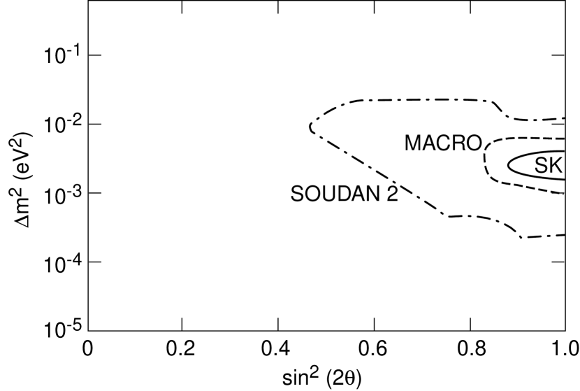
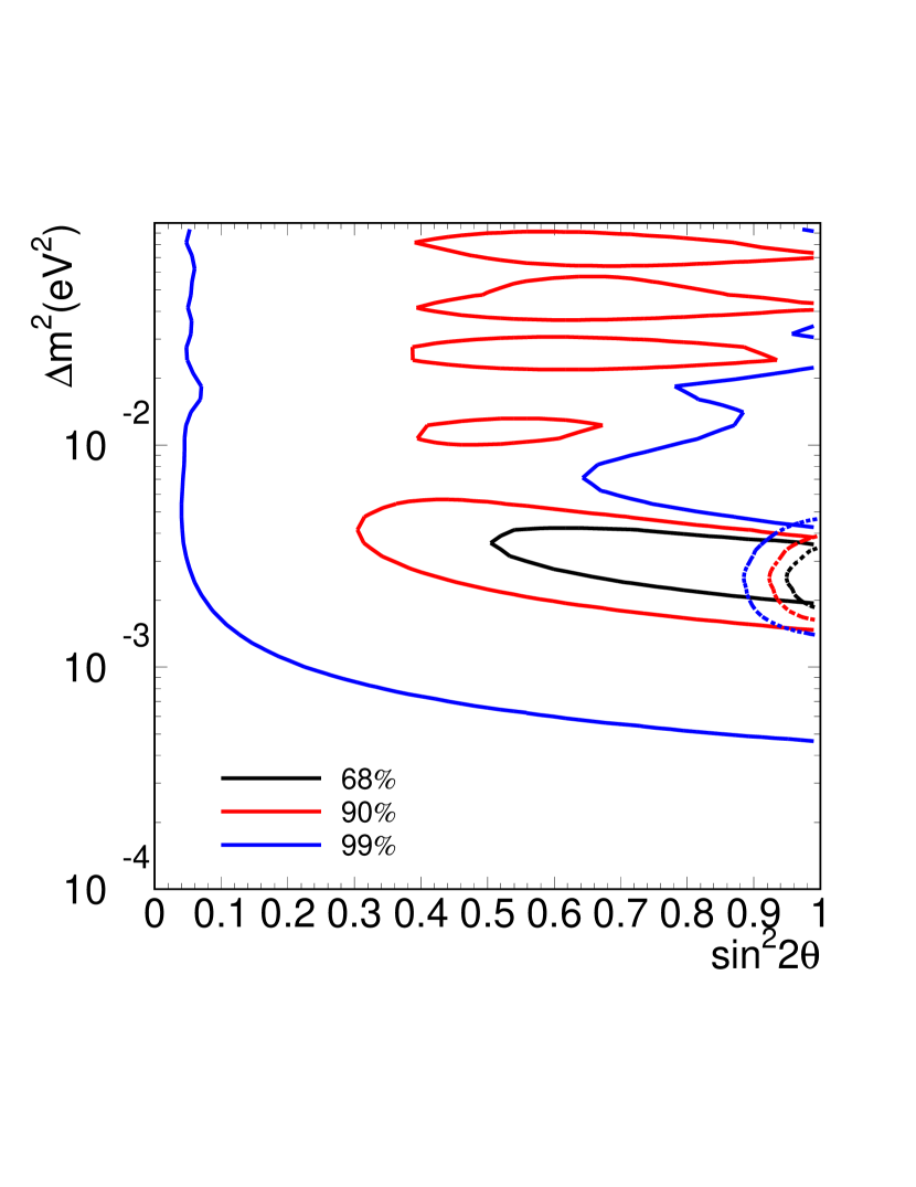
Figure 7: Left: 90% C.L. allowed region contours for $\nu_{\mu}\to\nu_{\tau}$ oscillations obtained by the Super-Kamiokande, MACRO and Soudan-2 experiments [29]. Right: Allowed region contours for $\nu_{\mu}$ disappearance obtained in the K2K experiment confronted with the allowed regions for $\nu_{\mu}\to\nu_{\tau}$ oscillations obtained in the Super-Kamiokande experiment [151].

The breakthrough in atmospheric neutrino research occurred in 1998, when the Super-Kamiokande Collaboration [3] discovered the up-down asymmetry of high-energy events generated by atmospheric $\nu_{\mu}$’s, providing a model independent proof of atmospheric $\nu_{\mu}$ disappearance. Indeed, on the basis of simple geometrical arguments the fluxes of upward-going and downward-going high-energy events generated by atmospheric $\nu_{\mu}$’s should be equal if nothing happens to neutrinos on their way from the production in the atmosphere to the detector (see Ref. [152]). The last published value of the measured up-down asymmetry is [149]

$$A_{\nu_{\mu}}^{\text{up-down}}(\text{SK})=\left(\frac{N_{\nu_{\mu}}^{\text{up}}-N_{\nu_{\mu}}^{\text{down}}}{N_{\nu_{\mu}}^{\text{up}}+N_{\nu_{\mu}}^{\text{down}}}\right)=-0.31\pm 0.04\,,$$ (4.26)

showing a $7\sigma$ evidence of disappearance of atmospheric high-energy upward-going muon neutrinos. These neutrinos travel a distance from about 2650 to about 12780 km ($0.2<\cos\theta<1$, where $\theta$ is the nadir angle of the neutrino trajectory), whereas the downward-going neutrinos travel a distance from about 20 to about 100 km ($-1<\cos\theta<-0.2$). Therefore, the simplest explanation of the atmospheric neutrino data is neutrino oscillations. The left panel in Fig. 6 shows the Super-Kamiokande up-down asymmetry as a function of momentum for $e$-like and $\mu$-like events generated, respectively, by atmospheric $\nu_{e}$, $\bar{\nu}_{e}$ and $\nu_{\mu}$, $\bar{\nu}_{\mu}$. One can see that there is a clear deficit of high-energy upward going muon neutrinos with respect to downward-going ones, which do not have time to oscillate. On the other hand, there is no up-down asymmetry at low energies because also most of the downward-going muon neutrinos have time to oscillate and a possible asymmetry is washed out by a poor correlation between the directions of the incoming neutrino and the observed charged lepton (the average angle between the two directions is $55^{\circ}$ at $p=400$ MeV and $20^{\circ}$ at 1.5 GeV [3]).

At the end of 2002 the long-baseline K2K experiment [6] confirmed the neutrino oscillation interpretation of the atmospheric neutrino anomaly observing the disappearance of accelerator $\nu_{\mu}$’s with average energy energy $\overline{E}\simeq 1.3\,\text{GeV}$ traveling 250 km from KEK to the Super-Kamiokande detector (only 56 of the $80.1{}^{+6.2}_{-5.4}$ expected events were observed).

The Super-Kamiokande atmospheric neutrino data and the data of the K2K experiment are well fitted by $\nu_{\mu}\to\nu_{\tau}$ transitions with the effective two-neutrino mixing parameters constrained in the ranges [153]

$$1.4\times 10^{-3}\,\text{eV}^{2}<\Delta{m}^{2}_{\text{ATM}}<5.1\times 10^{-3}\,\text{eV}^{2}\,,$$ (4.27)

$$\sin^{2}2\vartheta_{\text{ATM}}>0.86\,,$$ (4.28)

at 99.73% C.L. ($3\sigma$), with best-fit values

$$\Delta{m}^{2\,\text{bf}}_{\text{ATM}}=2.6\times 10^{-3}\,\text{eV}^{2}\,,\qquad\sin^{2}2\vartheta_{\text{ATM}}^{\text{bf}}=1\,.$$ (4.29)

Hence, the best-fit effective atmospheric mixing is maximal. The right panel in Fig. 6 shows the region in the $\sin^{2}2\vartheta_{\text{ATM}}$–$\Delta{m}^{2}_{\text{ATM}}$ plane for $\nu_{\mu}\to\nu_{\tau}$ oscillations allowed by Super-Kamiokande data [150]. The left panel in Fig. 7 shows the 90% C.L. allowed regions for $\nu_{\mu}\to\nu_{\tau}$ oscillations obtained in the MACRO and Soudan-2 experiments confronted with the corresponding region obtained in the Super-Kamiokande experiment [29]. The right panel in Fig. 7 shows the allowed regions for $\nu_{\mu}$ disappearance obtained in the K2K experiment confronted with the allowed regions for $\nu_{\mu}\to\nu_{\tau}$ oscillations obtained in the Super-Kamiokande experiment [151]. The left panel in Fig. 8 shows the allowed region obtained in Ref. [153] from the combined analysis of Super-Kamiokande atmospheric and K2K data.

Transitions of atmospheric $\nu_{\mu}$’s into $\nu_{e}$’s or sterile states are disfavored. The fraction $\sin^{2}\xi$ of atmospheric $\nu_{\mu}$’s that transform into sterile $\nu_{s}$ ($\nu_{\mu}\to\cos\xi\,\nu_{\tau}+\sin\xi\,\nu_{s}$) is limited at 90% C.L. by [154]

$$\sin^{2}\xi<0.19\,.$$ (4.30)

In the next years the MINOS [79] experiment will measure with improved precision the disappearance of muon neutrinos over a long-baseline of about 730 km. The OPERA [155] and ICARUS [156] experiments belonging to the CERN to Gran Sasso program (CNGS) [80] are aimed at a direct measurement of $\nu_{\mu}\to\nu_{\tau}$ oscillation over a similar long-baseline of about 730 km.

Figure 8: Left: Allowed region obtained from the analysis of Super-Kamiokande atmospheric and K2K data in terms of $\nu_{\mu}\to\nu_{\tau}$ oscillations [153]. Right: CHOOZ exclusion curves [139] confronted with the Kamiokande allowed regions [81].

4.3 The reactor experiment CHOOZ

CHOOZ was a long-baseline reactor $\nu_{e}$ disappearance experiment [157, 139, 77] which did not observe any disappearance of electron neutrinos at a distance of about 1 km from the source. In spite of such negative result, the CHOOZ experiment is very important, because it shows that the oscillations of electron neutrinos at the atmospheric scale of $\Delta{m}^{2}$ are small or zero. This constraint is particularly important in the framework of three-neutrino mixing, as will be discussed in Section 5. Therefore, we briefly review the results of the CHOOZ experiment.

The CHOOZ detector consisted in 5 tons of liquid scintillator in which neutrinos were revealed through the inverse $\beta$-decay reaction

$$\bar{\nu}_{e}+p\to n+e^{+}\,,$$ (4.31)

with a threshold $E_{\text{th}}=1.8\,\text{MeV}$. The neutrino energy is measured through the positron energy: $E=E_{e^{+}}-1.8\,\text{MeV}$. The detector was located at a distance of about 1 km from the Chooz power station, which has two pressurized-water reactors.

The ratio of observed and expected number of events in the CHOOZ experiment is

$$\frac{N^{\text{CHOOZ}}_{\text{observed}}}{N^{\text{CHOOZ}}_{\text{expected}}}=1.01\pm 0.04\,,$$ (4.32)

showing no indication of any electron antineutrino disappearance. The right panel in Fig. 8 [139] shows the CHOOZ exclusion curves confronted with the Kamiokande allowed regions for $\nu_{\mu}\to\nu_{e}$ transitions [81]. The area on the right of the exclusion curves is excluded. Since the Kamiokande allowed region lies in the excluded area, the disappearance of muon neutrinos observed in Kamiokande (and IMB, Super-Kamiokande, Soudan-2 and MACRO) cannot be due to $\nu_{\mu}\to\nu_{e}$ transitions. Indeed, $\nu_{\mu}\to\nu_{e}$ transitions are also disfavored by Super-Kamiokande data, which prefer the $\nu_{\mu}\to\nu_{\tau}$ channel [154] (therefore, the Super-Kamiokande collaboration did not calculate an allowed region for $\nu_{\mu}\to\nu_{e}$ transitions and the CHOOZ collaboration correctly compared their exclusion curve with the regions allowed by the results of the Kamiokande experiment).

The results of the CHOOZ experiment have been confirmed, albeit with lower accuracy, by the Palo Verde experiment [78].

5 Phenomenology of three-neutrino mixing

The solar and atmospheric evidences of neutrino oscillations are nicely accommodated in the minimal framework of three-neutrino mixing, in which the three flavor neutrinos $\nu_{e}$, $\nu_{\mu}$, $\nu_{\tau}$ are unitary linear combinations of three neutrinos $\nu_{1}$, $\nu_{2}$, $\nu_{3}$ with masses $m_{1}$, $m_{2}$, $m_{3}$, according to Eq. (2.46). As explained in Section 2 this scenario is theoretically motivated by the see-saw mechanism, which also predicts that massive neutrinos are Majorana particles.

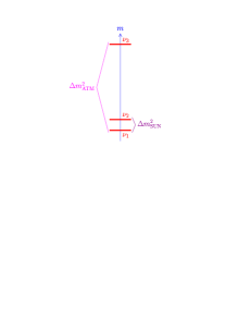
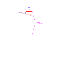
normal		inverted

Figure 9: The two three-neutrino schemes allowed by the hierarchy $\Delta{m}^{2}_{\text{SUN}}\ll\Delta{m}^{2}_{\text{ATM}}$.

5.1 Three-neutrino mixing schemes

Figure 9 shows the two three-neutrino schemes allowed by the observed hierarchy of squared-mass differences, $\Delta{m}^{2}_{\text{SUN}}\ll\Delta{m}^{2}_{\text{ATM}}$, with the massive neutrinos labeled in order to have

$$\Delta{m}^{2}_{\text{SUN}}=\Delta{m}^{2}_{21}\,,\quad\Delta{m}^{2}_{\text{ATM}}\simeq|\Delta{m}^{2}_{31}|\simeq|\Delta{m}^{2}_{32}|\,.$$ (5.1)

The two schemes in Fig. 9 are usually called “normal” and “inverted”, because in the normal scheme the smallest squared-mass difference is generated by the two lightest neutrinos and a natural neutrino mass hierarchy can be realized if $m_{1}\ll m_{2}$, whereas in the inverted scheme the smallest squared-mass difference is generated by the two heaviest neutrinos, which are almost degenerate for any value of the lightest neutrino mass $m_{3}$. This is shown in Fig. 10, where we have depicted the allowed ranges (between the dashed and dotted lines) for the neutrino masses obtained from the allowed values of $\Delta{m}^{2}_{\text{SUN}}$ in Eq. (4.16) and $\Delta{m}^{2}_{\text{ATM}}$ in Eq. (4.27), as functions of the lightest mass in the normal and inverted schemes. The solid lines correspond to the best fit values of $\Delta{m}^{2}_{\text{SUN}}$ and $\Delta{m}^{2}_{\text{ATM}}$ in Eqs. (4.18) and (4.29), respectively. One can see that at least two neutrinos have masses larger than about $7\times 10^{-3}\,\text{eV}$.

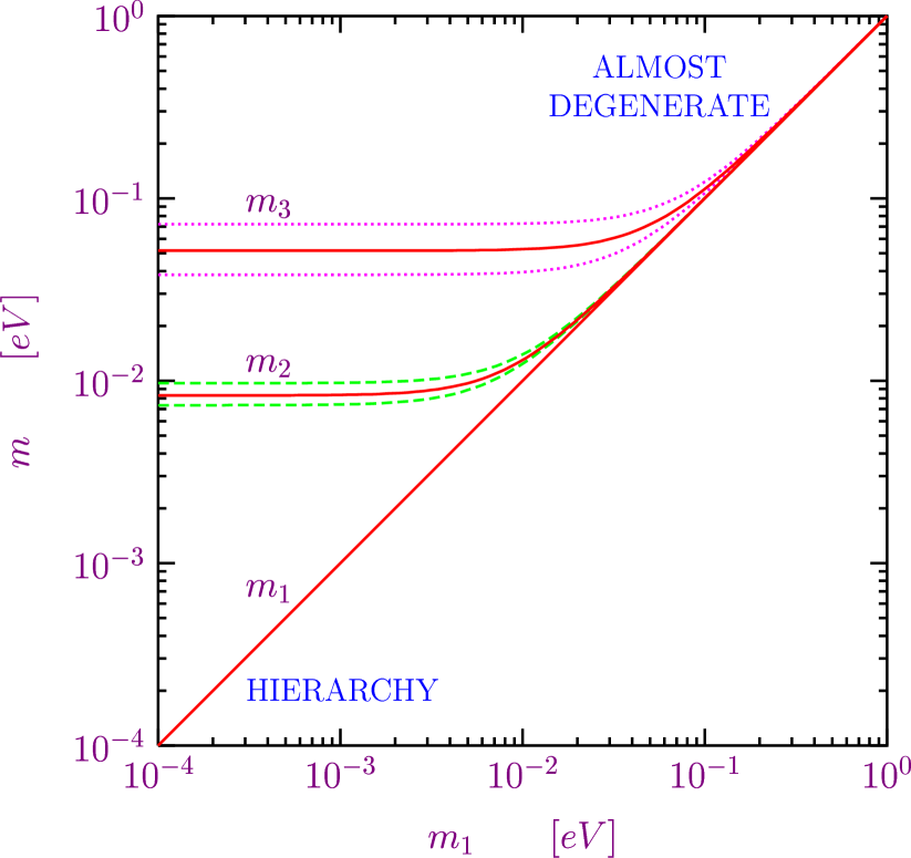
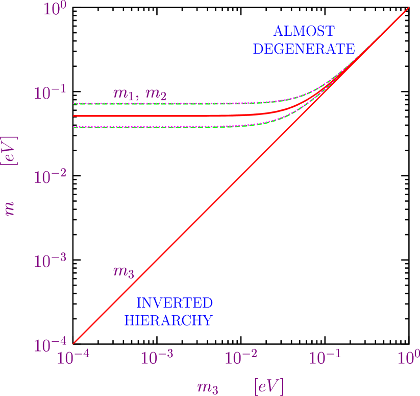
Figure 10: Allowed ranges for the neutrino masses as functions of the lightest mass $m_{1}$ and $m_{3}$ in the normal and inverted three-neutrino scheme, respectively.

In the case of three-neutrino mixing there are no light sterile neutrinos, in agreement with the absence of any indication in favor of active–sterile transitions in both solar and atmospheric neutrino experiments. Let us however emphasize that three-neutrino mixing cannot explain the indications in favor of short-baseline $\bar{\nu}_{\mu}\to\bar{\nu}_{e}$ transitions observed in the LSND experiment [75], which are presently under investigation in the MiniBooNE experiment [119].

Let us now discuss the current information on the three-neutrino mixing matrix $U$. In solar neutrino experiments $\nu_{\mu}$ and $\nu_{\tau}$ are indistinguishable, because the energy is well below $\mu$ and $\tau$ production and $\nu_{\mu}$, $\nu_{\tau}$ can be detected only through flavor-blind neutral-current interactions. Hence, solar neutrino oscillations, as well as the oscillations in the KamLAND experiment, depend only on the absolute value of the elements in the first row of the mixing matrix, $|U_{e1}|$, $|U_{e2}|$, $|U_{e3}|$ which regulates $\nu_{e}$ and $\bar{\nu}_{e}$ disappearance. Indeed, the survival probability of solar electron neutrinos can be written as [159]

$$\overline{P}_{\nu_{e}\to\nu_{e}}^{\,\text{sun}}=\left(1-|U_{e3}|^{2}\right)^{2}\overline{P}_{\nu_{e}\to\nu_{e}}^{\,\text{sun, (1,2)}}+|U_{e3}|^{4}\,,$$ (5.2)

where $\overline{P}_{\nu_{e}\to\nu_{e}}^{\,\text{sun, (1,2)}}$ is the two-neutrino survival probability in matter (3.50) calculated with the charged-current matter potential $V_{\text{CC}}$ multiplied by $(1-|U_{e3}|^{2})$ and $\vartheta=\vartheta_{12}$ in the parameterization (2.48) of the mixing matrix.

The hierarchy $\Delta{m}^{2}_{\text{SUN}}\ll\Delta{m}^{2}_{\text{ATM}}$ implies that neutrino oscillations generated by $\Delta{m}^{2}_{\text{ATM}}$ depend only on the absolute value of the elements in the last column of the mixing matrix, $|U_{e3}|$, $|U_{\mu 3}|$, $|U_{\tau 3}|$ because $m_{1}$ and $m_{2}$ are indistinguishable. Indeed, taking into account also the matter effects in the earth, the evolution equation of the neutrino amplitudes is given by Eq. (3.27) with $\Delta{m}^{2}_{k1}\simeq\Delta{m}^{2}_{31}\delta_{k3}$, leading to

$$i\,\frac{\text{d}}{\text{d}x}\,\psi_{\alpha\beta}(x)=\sum_{\rho}\left(U_{\beta 3}\,\frac{\Delta{m}^{2}_{31}}{2E}\,U_{\rho 3}^{*}+\delta_{\beta e}\,\delta_{\rho e}\,V_{\text{CC}}\right)\psi_{\alpha\rho}(x)\,,$$ (5.3)

which clearly depends only on the elements $U_{e3}$, $U_{\mu 3}$ and $U_{\tau 3}$ of the mixing matrix. In order to further demonstrate that only the absolute values $|U_{e3}|$, $|U_{\mu 3}|$, $|U_{\tau 3}|$ are relevant, we notice that in the parameterization (2.48) of the mixing matrix we have $U_{\beta 3}=|U_{\beta 3}|e^{-i\varphi_{13}\delta_{\beta e}}$, and Eq. (5.3) can be written as

$$i\,\frac{\text{d}}{\text{d}x}\,\psi_{\alpha\beta}(x)=e^{-i\varphi_{13}\delta_{\beta e}}\sum_{\rho}\left(|U_{\beta 3}|\,\frac{\Delta{m}^{2}_{31}}{2E}\,|U_{\rho 3}|+\delta_{\beta e}\,\delta_{\rho e}\,V_{\text{CC}}\right)e^{i\varphi_{13}\delta_{\rho e}}\,\psi_{\alpha\rho}(x)\,.$$ (5.4)

Since the flavor transition probabilities depend on the squared absolute value of the flavor amplitudes (see Eq. (3.26)), we can change arbitrarily the phases of the flavor amplitudes. Making the change of phase

$$\psi_{\alpha\beta}(x)\to e^{-i\varphi_{13}\delta_{\beta e}}\,\psi_{\alpha\beta}(x)\,,$$ (5.5)

we obtain the evolution equation

$$i\,\frac{\text{d}}{\text{d}x}\,\psi_{\alpha\beta}(x)=\sum_{\rho}\left(|U_{\beta 3}|\,\frac{\Delta{m}^{2}_{31}}{2E}\,|U_{\rho 3}|+\delta_{\beta e}\,\delta_{\rho e}\,V_{\text{CC}}\right)\psi_{\alpha\rho}(x)\,,$$ (5.6)

which depends only on $|U_{e3}|$, $|U_{\mu 3}|$ and $|U_{\tau 3}|$.

The only connection between solar and atmospheric oscillations is due to $|U_{e3}|$. Therefore, any information on the value of $|U_{e3}|$ is of crucial importance.

The key experiment for the determination of $|U_{e3}|$ has been the CHOOZ long-baseline reactor $\bar{\nu}_{e}$ disappearance experiment [157, 139, 77], which did not observe any disappearance at a distance of about 1 km from the reactor source (see Section 4.3). The negative result of the CHOOZ experiment, confirmed by the Palo Verde experiment [78], implies that the oscillations of electron neutrinos at the atmospheric scale are very small or even zero. The CHOOZ bound on the effective mixing angle (see Refs. [160, 21])

$$\sin^{2}2\vartheta_{\text{CHOOZ}}=4\,|U_{e3}|^{2}\left(1-|U_{e3}|^{2}\right)$$ (5.7)

implies that $|U_{e3}|$ is small:

$$|U_{e3}|^{2}<5\times 10^{-2}\,,$$ (5.8)

at 99.73% C.L. [161]. Therefore, solar and atmospheric neutrino oscillations are practically decoupled [160] and the effective mixing angles in solar, atmospheric and CHOOZ experiments can be related to the elements of the three-neutrino mixing matrix by (see also Ref. [162])

$$\sin^{2}\vartheta_{\text{SUN}}=\frac{|U_{e2}|^{2}}{1-|U_{e3}|^{2}}\,,\qquad\sin^{2}\vartheta_{\text{ATM}}=|U_{\mu 3}|^{2}\,,\qquad\sin^{2}\vartheta_{\text{CHOOZ}}=|U_{e3}|^{2}\,.$$ (5.9)

Taking into account the best-fit values of $\vartheta_{\text{SUN}}$ and $\vartheta_{\text{ATM}}$ in Eqs. (4.18) and (4.29), respectively, and

$$\sin^{2}\vartheta_{\text{CHOOZ}}^{\text{bf}}=0\,,$$ (5.10)

the best-fit value for the mixing matrix $U$ is

$$U_{\text{bf}}\simeq\left(\begin{smallmatrix}0.84&0.55&0.00\\ -0.39&0.59&0.71\\ 0.39&-0.59&0.71\end{smallmatrix}\right)\,.$$ (5.11)

Using the 99.73% C.L. allowed ranges for $\vartheta_{\text{SUN}}$, $\vartheta_{\text{ATM}}$ and $\vartheta_{\text{CHOOZ}}$ given by Eqs. (4.17), (4.28) and (5.8), respectively, we have reconstructed the allowed ranges for the elements of the mixing matrix:

$$|U|\simeq\left(\begin{smallmatrix}0.76-0.88&0.47-0.62&0.00-0.22\\ 0.09-0.62&0.29-0.79&0.55-0.85\\ 0.11-0.62&0.32-0.80&0.51-0.83\end{smallmatrix}\right)\,.$$ (5.12)

Such mixing matrix, with all elements large except $U_{e3}$, is called “bilarge”. It is very different from the quark mixing matrix, in which mixing is very small. This difference is an important piece of information for our understanding of the physics beyond the Standard Model, which presumably involves some sort of quark-lepton unification.

An important open problem is the determination of the absolute values of neutrino masses. The most sensitive known ways to probe the absolute values of neutrino masses are the observation of the end-point part of the electron spectrum in Tritium $\beta$-decay, the observation of large-scale structures in the early universe and the search for neutrinoless double-$\beta$ decay, if neutrinos are Majorana particles (we do not consider here the interesting possibility to determine neutrino masses through the observation of supernova neutrinos; see Ref. [35] and references therein).

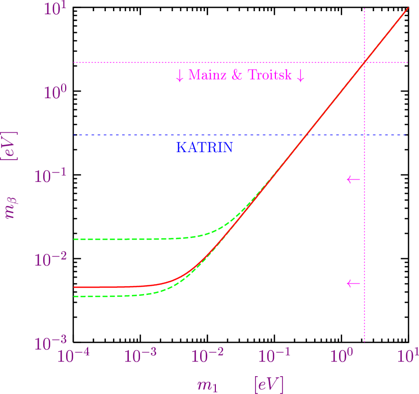
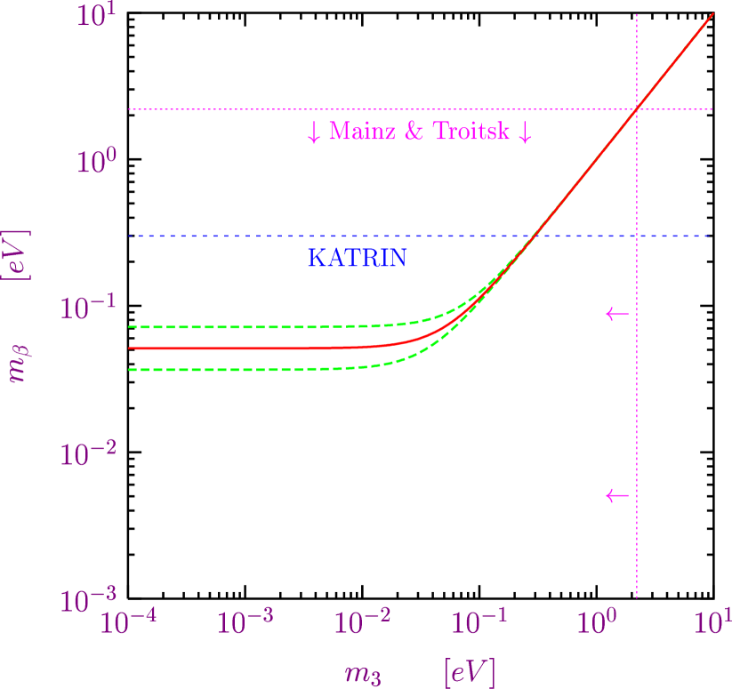
Figure 11: Effective neutrino mass $m_{\beta}$ in Tritium $\beta$-decay experiments as a function of the lightest mass $m_{1}$ and $m_{3}$ in the normal and inverted three-neutrino scheme, respectively.

5.2 Tritium $\beta$-decay

Up to now, no indication of a neutrino mass has been found in Tritium $\beta$-decay experiments, leading to the 95% C.L. upper limit [163]

$$m_{\beta}<2.2\,\text{eV}$$ (5.13)

on the effective mass

$$m_{\beta}=\sqrt{\sum_{k}|U_{ek}|^{2}m_{k}^{2}}\,,$$ (5.14)

obtained in the Mainz [164] and Troitsk [165] experiments. After 2007, the KATRIN experiment [166] will explore $m_{\beta}$ down to about $0.2-0.3\,\text{eV}$. Figure 11 shows the allowed range (between the dashed lines) for $m_{\beta}$ obtained from the 99.73% C.L. allowed values of the oscillation parameters in Eqs. (4.16), (4.17), (4.27), (4.28), as a function of the lightest mass in the normal and inverted three-neutrino schemes. The solid line corresponds to the best fit values of the oscillation parameters in Eqs. (4.18) and (4.29). One can see that in the normal scheme with a mass hierarchy $m_{\beta}$ has a value between about $3\times 10^{-3}\,\text{eV}$ and $2\times 10^{-2}\,\text{eV}$, whereas in the inverted scheme $m_{\beta}$ is larger than about $3\times 10^{-2}\,\text{eV}$. Therefore, if in the future it will be possible to constraint $m_{\beta}$ to be smaller than about $3\times 10^{-2}\,\text{eV}$, a normal hierarchy of neutrino masses will be established.

From Figs. 10 and 11 it is clear that the bound (5.13) can be saturated only if the three neutrino masses are almost degenerate. In this case the dependence of $m_{k}$ on the index $k$ can be neglected in Eq. (5.14), leading to $m_{\beta}\simeq m_{k}$. Therefore, the upper limit for each mass is the same as the one on $m_{\beta}$ in Eq. (5.13): at 95% C.L.

$$m_{k}<2.2\,\text{eV}\,.$$ (5.15)

5.3 Cosmological bounds on neutrino masses

In the early hot universe neutrinos are in equilibrium in the primeval plasma through the weak interaction reactions $\nu\bar{\nu}\leftrightarrows e^{+}e^{-}$, $\overset{\scriptscriptstyle(-)}{\nu}e\leftrightarrows\overset{\scriptscriptstyle(-)}{\nu}e$, $\overset{\scriptscriptstyle(-)}{\nu}N\leftrightarrows\overset{\scriptscriptstyle(-)}{\nu}N$, $\nu_{e}n\leftrightarrows pe^{-}$, $\bar{\nu}_{e}p\leftrightarrows ne^{+}$, $n\leftrightarrows pe^{-}\bar{\nu}_{e}$. As the universe expands and cools, the rate of weak interactions decreases. When the temperature of the Universe goes below $T\simeq 1\,\text{MeV}$, the mean neutrino free path becomes larger than the horizon and neutrinos practically cease to interact with the plasma. At $T\lesssim 0.5\,\text{MeV}$ electron and positron in the plasma annihilate into photons, increasing the photon temperature $T_{\gamma}$ with respect to the neutrino temperature $T_{\nu}$ by a factor $(11/4)^{1/3}$, easily calculated from entropy conservation (see Refs. [13, 14, 32]). From the well measured temperature of the Cosmic Microwave Background Radiation (CMBR) $T_{\gamma}=2.725\pm 0.001\,\text{K}$, we infer the neutrino temperature $T_{\nu}=1.945\pm 0.001\,\text{K}$, and $k\,T_{\nu}=1.676\pm 0.001\times 10^{-4}\,\text{eV}$. As we have seen in Section 5.1, at least two neutrinos have masses larger than about $7\times 10^{-3}\,\text{eV}$ (see Fig. 10). Hence, at least two massive neutrinos in the present relic neutrino background are non-relativistic. The number density of relic non-relativistic neutrinos can be calculated from the Fermi-Dirac distribution (see Refs. [13, 14, 32]):

$$n_{\nu_{k},\bar{\nu}_{k}}=\frac{3}{2}\,\frac{\zeta(3)}{\pi^{2}}T_{\nu}^{3}\simeq 0.1827\,T_{\nu}^{3}\simeq 112\,\text{cm}^{-3}\,,$$ (5.16)

with $\zeta(3)\simeq 1.202$. Their contribution to the present density of the universe (normalized to the critical density $\rho_{c}=3H^{2}/8\pi G_{\text{N}}$, where $H$ is the Hubble constant and $G_{\text{N}}$ is the Newton constant) is given by

$$\Omega_{k}=\frac{n_{\nu_{k},\bar{\nu}_{k}}\,m_{k}}{\rho_{c}}\simeq\frac{1}{h^{2}}\frac{m_{k}}{94.14\,\text{eV}}\,,$$ (5.17)

where $h$ is the value of the Hubble constant in units of $100\,\text{km}\,\text{s}^{-1}\,\text{Mpc}^{-1}$ (the current determination of $h$ from a global fit of cosmological data is $h=0.71{}^{+0.04}_{-0.03}$ [167]). The total contribution of relic neutrinos to the present density of the universe is given by [168, 169]

$$\Omega_{\nu}\,h^{2}=\frac{\sum_{k}m_{k}}{94.14\,\text{eV}}\,.$$ (5.18)

It is clear that, just from the need to avoid overclosing the Universe, the sum of neutrino masses has to be lighter than about 100 eV. If one further takes $h\lesssim 0.8$ and $\Omega_{\nu}\lesssim 0.1$, as indicated by astronomical data, one gets a quite restrictive upper bound of about 6 eV for the sum of neutrino masses.

An even stronger bound on the sum of neutrino masses follows from more sophisticated calculations of structure formation in the early universe. Neutrinos with masses of the order of 1 eV or lighter constitute what is called “hot dark matter”, which is dark matter that is now non-relativistic, but was relativistic at the time of matter-radiation equality, when the contribution of matter and radiation to the density of the universe was equal. Since the radiation energy density scales as $T^{4}$ and matter energy density scale as $T^{3}$, matter started to dominate the density of the universe and structures started to form after matter-radiation equality. However, hot dark matter particles did not participate to the beginning of structure formation at matter-radiation equality, but streamed freely until they become non relativistic. Hence, neutrinos contribute only to the formation of structures with size given by the free-streaming distance traveled by neutrinos until they become non relativistic. The formation of structures on smaller scales is suppressed with respect to a universe without hot dark matter. The absence of such suppression in the present astronomical observations of large scale structures (LSS) in the universe allow to put a strong upper bound on the sum of neutrino masses (see Refs. [170, 171, 172]).

The recent high-precision CMBR data of the WMAP satellite [173] combined with the LSS data of the 2dF Galaxy Redshift Survey (2dFGRS) [174] and other astronomical data (see Ref. [167]) allowed the WMAP collaboration to derive the impressive bound

$$\Omega_{\nu}h^{2}<0.0076\,,$$ (5.19)

with 95% confidence, which, using Eq. (5.18), yields

$$\sum_{k}m_{k}<0.71\,\text{eV}\,.$$ (5.20)

From the smallness of the squared-mass differences implied by solar and atmospheric neutrino data (see Eqs. (4.16), (4.27) and (5.1)), it is clear that the bound (5.20) can be saturated only if the three neutrino masses are almost degenerate. Therefore, the upper limit on each neutrino mass is one third of the bound in Eq.(5.20):

$$m_{k}<0.23\,\text{eV}\,.$$ (5.21)

This impressive limit is one order of magnitude more restrictive than the limit (5.15) obtained in Tritium experiments, reaching already the level of sensitivity of the future KATRIN experiment. Let us emphasize, however, that the KATRIN experiment is important in order to probe the neutrino masses in a model-independent way. Indeed, the cosmological bound relies on several assumptions on the cosmological model and some controversial data (see the discussion in Ref. [175] and Ref. [176] for an alternative model). Using only the WMAP and 2dFGRS data, the author of Ref. [177] found the 95% confidence limit

$$\sum_{k}m_{k}<2.12\,\text{eV}\,.$$ (5.22)

Adding also the Hubble Space Telescope determination of $h$, the authors of Ref. [178] obtained the 95% confidence limit

$$\sum_{k}m_{k}<1.1\,\text{eV}\,.$$ (5.23)

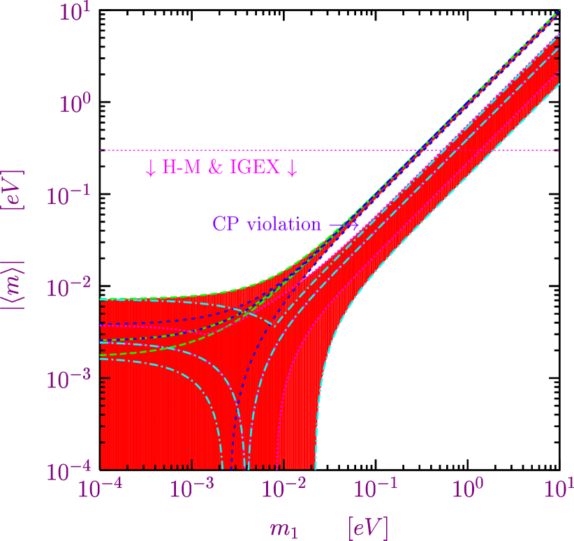
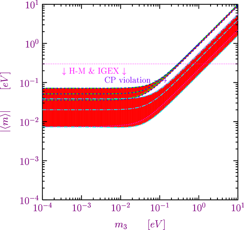
Figure 12: Effective Majorana mass $|\langle{m}\rangle|$ in neutrinoless double-$\beta$ decay experiments as a function of the lightest mass $m_{1}$ and $m_{3}$ in the normal and inverted three-neutrino scheme, respectively.

5.4 Neutrinoless double-$\beta$ decay

A very important open problem in neutrino physics is the Dirac or Majorana nature of neutrinos. From the theoretical point of view it is expected that neutrinos are Majorana particles, with masses generated by the see-saw mechanism (see Section 2.4) or by effective Lagrangian terms in which heavy degrees of freedom have been integrated out (see Section 2.5 and Ref. [38]).

The best known way to search for Majorana neutrino masses is neutrinoless double-$\beta$ decay, whose amplitude is proportional to the effective Majorana mass (see Refs. [13, 14, 17, 21, 31])

$$|\langle{m}\rangle|=\bigg{|}\sum_{k}U_{ek}^{2}\,m_{k}\bigg{|}\,.$$ (5.24)

The present experimental upper limit on $|\langle{m}\rangle|$, between about 0.3 eV and 1.3 eV, has been obtained in the Heidelberg-Moscow [179] and IGEX experiments [180]. The large uncertainty is due to the difficulty of calculating the nuclear matrix element in the decay. Figure 12 shows the allowed range for $|\langle{m}\rangle|$ obtained from the 99.73% C.L. allowed values of the oscillation parameters in Eqs. (4.16), (4.17), (4.27), (4.28), as a function of the lightest mass in the normal and inverted three-neutrino schemes (see also Refs. [181, 182, 183]). If CP is conserved, $|\langle{m}\rangle|$ is constrained to lie in the shadowed region. Finding $|\langle{m}\rangle|$ in an unshaded strip would signal CP violation. One can see that in the normal scheme large cancellations between the three mass contributions are possible and $|\langle{m}\rangle|$ can be arbitrarily small. On the other hand, the cancellations in the inverted scheme are limited, because $\nu_{1}$ and $\nu_{2}$, with which the electron neutrino has large mixing, are almost degenerate and much heavier than $\nu_{3}$. Since the solar mixing angle is less than maximal, a complete cancellation between the contributions of $\nu_{1}$ and $\nu_{2}$ is excluded, leading to a lower bound of about $7\times 10^{-3}\,\text{eV}$ for $|\langle{m}\rangle|$ in the inverted scheme (see also Ref. [184]). If in the future $|\langle{m}\rangle|$ will be found to be smaller than about $7\times 10^{-3}\,\text{eV}$, it will be established that either neutrinos have a mass hierarchy or they are Dirac particles. Many neutrinoless double-$\beta$ decay experiments are planned for the future (see Refs. [185, 35, 186, 187]). The most sensitive may be able to probe such small values of $|\langle{m}\rangle|$.

6 Future prospects

As reviewed in Section 4, in recent years neutrino oscillations have been established in a model-independent way in solar ($\sim 19\sigma$) and atmospheric ($\sim 7\sigma$) neutrino experiments. An impressive proof of neutrino oscillations has also been obtained in the KamLAND reactor experiment ($\sim 4\sigma$). As we have discussed in Section 5, all these experimental results are nicely accommodated in the framework of three-neutrino mixing. Only the LSND anomaly [75] does not fit in this scheme, as already noticed. Its interpretation in terms of neutrino oscillation is presently under investigation in the MiniBooNE experiment [119].

Putting aside for the moment the controversial LSND anomaly, the immediate future prospects of neutrino oscillation research deal with the precise determination of the parameters of the three-neutrino mixing matrix. The actual value of $|U_{e3}|$, the real unknown, will be searched for in the near future with the long baseline accelerator neutrino programs MINOS [79, 188] in the United States, OPERA [189] and ICARUS [190] in Europe (CERN to Gran Sasso [80]) and JHF [191] in Japan. All these projects use conventional neutrino beams.

However, the evolution of neutrino physics demands new schemes to produce intense, collimated and pure neutrino beams. New possibilities have been studied in the last few years: neutrino beams from a Neutrino Factory, Beta-Beams and Super-Beams, that here we briefly summarize.

The current Neutrino Factory concept implies the production, collection, and storage of muons to produce very intense beams of muon and electron neutrinos with equal fluxes through the decays (4.21). Research and development addressing the feasibility of a Neutrino Factory are currently in progress. Review studies on the physics reach of the Neutrino Factory option are given in Refs. [192, 193]. Incidentally, we notice that anomalous muon decays, due to non standard weak interactions, if responsible of the observed LSND effect, could be easily tested at a Neutrino Factory with a short-baseline experiment, using a 10 ton detector capable of charge discrimination [125].

The Beta-Beam concept, first proposed in Ref. [194], is based on the acceleration and storage of radioactive ions. The $\beta$-decay of these radioactive ions can produce a very intense beam of electron neutrinos or antineutrinos with perfectly known energy spectrum. The physics reach of a CERN based Beta-Beam and of a Super-Beam+Beta-Beam combination is studied in Ref. [195]. In this study a Super-Beam is a very intense $\nu_{\mu}$ beam that has a Super Proton Linac (SPL) as injector delivering $10^{23}$ protons on target per year with energy of 2.2 GeV (see also Ref. [196]). The sensitivity to the Dirac CP-violating phase $\varphi_{13}$ in the neutrino mixing matrix (2.48) reachable in a Super-Beam+Beta-Beam combination results to be comparable to the sensitivity reachable in a Neutrino Factory if $\sin^{2}{\vartheta_{13}}\gtrsim 10^{-4}$. Comparisons between the sensitivities of different projects already approved or planned are presented in Ref. [197].

A next-generation neutrino oscillation experiment using reactor antineutrinos could give important information on the size of the mixing angle $\vartheta_{13}$ [198, 200]. Reactor experiments can give a clean measure of the mixing angle without ambiguities associated with the size of the other mixing angles, matter effects, and effects due to CP violation. The key question is whether a next-generation experiment can reach the needed sensitivity goals to make a measurement of $\sin^{2}2\vartheta_{13}$ at the $10^{-2}$ level [199, 200].

However, the search for $|U_{13}|$ and CP violation in the lepton sector does not cover all the items in today neutrino physics. Let us emphasize that still several fundamental characteristics of neutrinos are unknown. Among them, the Dirac or Majorana nature of neutrinos, the absolute scale of neutrino masses, the distinction between the normal and inverted schemes and the electromagnetic properties of neutrinos.

In our opinion the most important question in today neutrino physics is: are massive neutrinos Majorana particles? This question can be resolved with an affirmative answer if neutrinoless beta decay is observed [201, 202]. Many experimental proposals exist that will increase dramatically the sensitivity of the neutrinoless double-$\beta$ decay search, reaching $|\langle{m}\rangle|\sim 10^{-2}$ eV (see Refs. [185, 35, 186, 187]).

Besides masses, neutrinos can have magnetic moments (see Refs. [17, 13, 14, 36]). In the case of a Dirac neutrino, a large enough magnetic moment could lead to spin precession in a transverse magnetic field [203, 204, 205, 206], generating transitions between a neutrino with negative helicity and one with positive helicity, which is practically sterile. A Majorana neutrino cannot have a magnetic moment, but different Majorana neutrinos can have transition magnetic moments, which could lead to Spin-Flavor Precession (SFP). However, SFP is suppressed in vacuum by the mass difference of different neutrinos. In 1988 Akhmedov [207, 208] and Lim and Marciano [209] discovered that the mass difference can be compensated by the matter potential for neutrinos propagating in a medium, leading to the so-called Resonant Spin-Flavor Precession (RSFP) mechanism, which is analogous to the MSW effect.

The RSFP mechanism was proposed as a possible explanation of the solar neutrino problem and was considered a viable possibility for many years. Now we know that the solar neutrino problem is due to neutrino oscillations (see Section 4.1), but RSFP could still be a subdominant mechanism (see Ref. [210]). A possible signature of RSFP would be a periodic variability of the solar neutrino flux due to temporal variations of the magnetic field or to the inclination of the solar equator with respect to the ecliptic. A recent analysis of Super-Kamiokande data put severe limits to possible periodic modulations of the ${}^{8}\text{B}$ solar neutrino flux [211] (see, however, Ref. [212] for a different point of view).

If massive neutrinos are Majorana particles, a combination of the RSFP mechanism and oscillations can induce besides $\nu_{e}\to\nu_{\mu},\nu_{\tau},\bar{\nu}_{\mu},\bar{\nu}_{\tau}$ transitions also $\nu_{e}\to\bar{\nu}_{e}$ transitions of solar neutrinos [213, 214, 215], which can be observed in solar neutrino detectors through the inverse $\beta$-decay process (4.31). However, the Super-Kamiokande experiment did not find any indication of $\bar{\nu}_{e}$’s coming from the sun and established an upper limit of $8\times 10^{-3}$ for the averaged probability of $\nu_{e}\to\bar{\nu}_{e}$ conversion in the energy range 8-20 MeV (assuming the initial Standard Solar Model ${}^{8}\text{B}$ $\nu_{e}$ flux) [216].

In any case, even if at the moment there seems to be no indication of an effect of the RSFP mechanism in solar neutrino data, it is important to pursue this line of research, because magnetic moments are important properties and the existence of large neutrino magnetic moments could give crucial indications on the physics beyond the Standard Model.

Direct measurements of neutrino magnetic moments are also planned: a proposal on the direct detection of antineutrino-electron scattering with an artificial tritium source [217] will search for a neutrino magnetic moment about two orders of magnitude smaller than the present-day laboratory upper limit, reaching a sensitivity of about $10^{-12}\,\mu_{\text{B}}$, where $\mu_{\text{B}}$ is the Bohr magneton.

7 Conclusions

The recent years have been extraordinarily fruitful for neutrino physics, yielding model-independent proofs of solar and atmospheric neutrino oscillations, which have been confirmed, respectively, by the reactor experiment KamLAND and the accelerator experiment K2K. Taking into account the negative result of the CHOOZ long-baseline reactor $\bar{\nu}_{e}$ disappearance experiment, the global fit of solar, KamLAND, atmospheric and K2K data have provided important information on the neutrino mixing parameters in the framework of three-neutrino mixing, which is predicted by the natural versions of the see-saw mechanism.

The only experimental result that cannot be explained in the framework of three-neutrino mixing is the controversial indication in favor of short-baseline $\bar{\nu}_{\mu}\to\bar{\nu}_{e}$ transitions observed in the LSND experiment. It is very important that the MiniBooNE experiment running at Fermilab will check the validity of the LSND indication in the near future. If MiniBooNE will obtain a positive result, the investigation of new possibilities (as four-neutrino mixing, CPT violation, etc.) will become imperative. These new phenomena would be very interesting for our understanding of the physics beyond the Standard Model.

Even if the values of some parameters of three-neutrino mixing are determined with a precision that was unthinkable a few years ago, still several fundamental characteristics of neutrinos remain unknown. Among them the most important are: the Dirac or Majorana nature of neutrinos, the absolute scale of neutrino masses, the distinction between the normal and inverted schemes, the value of $|U_{e3}|$, the existence of CP violation in the lepton sector, the number of light neutrinos and the electromagnetic properties of neutrinos. Several existing experiments and future projects are aimed at the exploration of these characteristics, which are very important for our understanding of neutrino physics. Their determination is likely to shed some light on the new physics beyond the Standard Model. Therefore, we think that interesting years lie ahead in neutrino physics research.

References

- [1] B. Pontecorvo, Sov. Phys. JETP 6 (1957) 429 [Zh. Eksp. Teor. Fiz. 33 (1957) 549].
- [2] B. Pontecorvo, Sov. Phys. JETP 7 (1958) 172 [Zh. Eksp. Teor. Fiz. 34 (1958) 247].
- [3] Super-Kamiokande, Y. Fukuda et al., Phys. Rev. Lett. 81 (1998) 1562, hep-ex/9807003.
- [4] Kamiokande-II, K.S. Hirata et al., Phys. Lett. B205 (1988) 416.
- [5] IMB, R.M. Bionta et al., Phys. Rev. D38 (1988) 768.
- [6] K2K, M.H. Ahn et al., Phys. Rev. Lett. 90 (2003) 041801, hep-ex/0212007.
- [7] SNO, Q.R. Ahmad et al., Phys. Rev. Lett. 87 (2001) 071301, nucl-ex/0106015.
- [8] Super-Kamiokande, S. Fukuda et al., Phys. Rev. Lett. 86 (2001) 5651, hep-ex/0103032.
- [9] Homestake, B.T. Cleveland et al., Astrophys. J. 496 (1998) 505.
- [10] SNO, Q.R. Ahmad et al., Phys. Rev. Lett. 89 (2002) 011301, nucl-ex/0204008.
- [11] SNO, S. Ahmed et al., nucl-ex/0309004.
- [12] KamLAND, K. Eguchi et al., Phys. Rev. Lett. 90 (2003) 021802, hep-ex/0212021.
- [13] R.N. Mohapatra and P.B. Pal, Massive neutrinos in physics and astrophysics (World Sci. Lect. Notes Phys. 60, 1998).
- [14] C.W. Kim and A. Pevsner, Neutrinos in physics and astrophysics (Harwood Academic Press, Chur, Switzerland, 1993), Contemporary Concepts in Physics, Vol. 8.
- [15] J.N. Bahcall, Neutrino Astrophysics (Cambridge University Press, 1989).
- [16] S.M. Bilenky and B. Pontecorvo, Phys. Rept. 41 (1978) 225.
- [17] S.M. Bilenky and S.T. Petcov, Rev. Mod. Phys. 59 (1987) 671.
- [18] S.P. Mikheev and A.Y. Smirnov, Sov. Phys. Usp. 30 (1987) 759.
- [19] T.K. Kuo and J. Pantaleone, Rev. Mod. Phys. 61 (1989) 937.
- [20] V. Castellani et al., Phys. Rept. 281 (1997) 309, astro-ph/9606180.
- [21] S.M. Bilenky, C. Giunti and W. Grimus, Prog. Part. Nucl. Phys. 43 (1999) 1, hep-ph/9812360.
- [22] G. Altarelli and F. Feruglio, Phys. Rept. 320 (1999) 295, hep-ph/9905536.
- [23] T. Kajita and Y. Totsuka, Rev. Mod. Phys. 73 (2001) 85.
- [24] C.K. Jung et al., Ann. Rev. Nucl. Part. Sci. 51 (2001) 451.
- [25] M.F. Altmann, R.L. Mossbauer and L.J.N. Oberauer, Rept. Prog. Phys. 64 (2001) 97.
- [26] S.M. Bilenky and C. Giunti, Int. J. Mod. Phys. A16 (2001) 3931, hep-ph/0102320.
- [27] M. Beuthe, Phys. Rept. 375 (2003) 105, hep-ph/0109119.
- [28] T.K. Gaisser and M. Honda, Ann. Rev. Nucl. Part. Sci. 52 (2002) 153, hep-ph/0203272.
- [29] G. Giacomelli, M. Giorgini and M. Spurio, hep-ex/0201032.
- [30] M. Gonzalez-Garcia and Y. Nir, Rev. Mod. Phys. 75 (2003) 345, hep-ph/0202058.
- [31] S.R. Elliott and P. Vogel, Ann. Rev. Nucl. Part. Sci. 52 (2002) 115, hep-ph/0202264.
- [32] A.D. Dolgov, Phys. Rept. 370 (2002) 333, hep-ph/0202122.
- [33] B. Kayser, hep-ph/0211134.
- [34] L. Miramonti and F. Reseghetti, La Rivista del Nuovo Cimento 25 (2002) 1, hep-ex/0302035.
- [35] S.M. Bilenky et al., Phys. Rept. 379 (2003) 69, hep-ph/0211462.
- [36] W. Grimus, hep-ph/0307149.
- [37] C. Giunti and M. Laveder, hep-ph/0301276.
- [38] G. Altarelli and F. Feruglio, hep-ph/0306265.
- [39] C. Giunti and M. Laveder, Neutrino Unbound, http://www.nu.to.infn.it.
- [40] S.L. Glashow, Nucl. Phys. 22 (1961) 579.
- [41] S. Weinberg, Phys. Rev. Lett. 19 (1967) 1264.
- [42] A. Salam, (1969), Proc. of the 8th Nobel Symposium on Elementary particle theory, relativistic groups and analyticity, Stockholm, Sweden, 1968, edited by N. Svartholm, p.367-377.
- [43] L. Landau, Nucl. Phys. 3 (1957) 127.
- [44] T.D. Lee and C.N. Yang, Phys. Rev. 105 (1957) 1671.
- [45] A. Salam, Nuovo Cim. 5 (1957) 299.
- [46] E. Majorana, Nuovo Cim. 14 (1937) 171.
- [47] T. Yanagida, (1979), Proc. of the Workshop on Unified Theory and the Baryon Number of the Universe, KEK, Japan.
- [48] M. Gell-Mann, P. Ramond and R. Slansky, (1979), In ’Supergravity’, p. 315, edited by F. van Nieuwenhuizen and D. Freedman, North Holland, Amsterdam.
- [49] R.N. Mohapatra and G. Senjanovic, Phys. Rev. Lett. 44 (1980) 912.
- [50] S. Weinberg, Phys. Rev. Lett. 43 (1979) 1566.
- [51] S. Weinberg, Phys. Rev. D22 (1980) 1694.
- [52] H.A. Weldon and A. Zee, Nucl. Phys. B173 (1980) 269.
- [53] Particle Data Group, K. Hagiwara et al., Phys. Rev. D66 (2002) 010001.
- [54] S.S. Bulanov et al., hep-ph/0301268.
- [55] K. Belotsky et al., Phys. Rev. D68 (2003) 054027, hep-ph/0210153.
- [56] F.D. Murnaghan, The unitary and rotation groups (Spartan Articles, Washington D.C., 1962).
- [57] J. Schechter and J.W.F. Valle, Phys. Rev. D21 (1980) 309.
- [58] J. Schechter and J.W.F. Valle, Phys. Rev. D22 (1980) 2227.
- [59] C. Giunti, C.W. Kim and M. Monteno, Nucl. Phys. B521 (1998) 3, hep-ph/9709439.
- [60] C. Giunti and M. Tanimoto, Phys. Rev. D66 (2002) 113006, hep-ph/0209169.
- [61] GALLEX, W. Hampel et al., Phys. Lett. B447 (1999) 127.
- [62] SAGE, J.N. Abdurashitov et al., J. Exp. Theor. Phys. 95 (2002) 181, astro-ph/0204245.
- [63] GNO, M. Altmann et al., Phys. Lett. B490 (2000) 16, hep-ex/0006034.
- [64] Bugey, Y. Declais et al., Nucl. Phys. B434 (1995) 503.
- [65] CHOOZ, M. Apollonio et al., Phys. Lett. B466 (1999) 415, hep-ex/9907037.
- [66] Super-Kamiokande, S. Fukuda et al., Phys. Lett. B539 (2002) 179, hep-ex/0205075.
- [67] Super-Kamiokande, M. Smy et al., hep-ex/0309011.
- [68] C. Giunti, C.W. Kim and U.W. Lee, Phys. Rev. D45 (1992) 2414.
- [69] C. Giunti and C.W. Kim, Found. Phys. Lett. 14 (2001) 213, hep-ph/0011074.
- [70] C. Giunti, hep-ph/0302026.
- [71] CDHS, F. Dydak et al., Phys. Lett. B134 (1984) 281.
- [72] CCFR/NuTeV, D. Naples et al., Phys. Rev. D59 (1999) 031101, hep-ex/9809023.
- [73] CHORUS, E. Eskut et al., Phys. Lett. B497 (2001) 8.
- [74] NOMAD, P. Astier et al., Phys. Lett. B570 (2003) 19, hep-ex/0306037.
- [75] LSND, A. Aguilar et al., Phys. Rev. D64 (2001) 112007, hep-ex/0104049.
- [76] KARMEN, B. Armbruster et al., Phys. Rev. D65 (2002) 112001, hep-ex/0203021.
- [77] CHOOZ, M. Apollonio et al., Eur. Phys. J. C27 (2003) 331, hep-ex/0301017.
- [78] Palo Verde, F. Boehm et al., Phys. Rev. D64 (2001) 112001, hep-ex/0107009.
- [79] MINOS, M.V. Diwan, eConf C0209101 (2002) TH08, hep-ex/0211026.
- [80] D. Duchesneau, eConf C0209101 (2002) TH09, hep-ex/0209082.
- [81] Kamiokande, Y. Fukuda et al., Phys. Lett. B335 (1994) 237.
- [82] IMB, R. Becker-Szendy et al., Phys. Rev. D46 (1992) 3720.
- [83] Soudan 2, M. Sanchez et al., hep-ex/0307069.
- [84] MACRO, M. Ambrosio et al., Phys. Lett. B566 (2003) 35, hep-ex/0304037.
- [85] Kamiokande, Y. Fukuda et al., Phys. Rev. Lett. 77 (1996) 1683.
- [86] L. Wolfenstein, Phys. Rev. D17 (1978) 2369.
- [87] C. Giunti, C.W. Kim and U.W. Lee, Phys. Lett. B274 (1992) 87.
- [88] P. Langacker, J.P. Leveille and J. Sheiman, Phys. Rev. D27 (1983) 1228.
- [89] S.P. Mikheev and A.Y. Smirnov, Nuovo Cim. C9 (1986) 17.
- [90] H.A. Bethe, Phys. Rev. Lett. 56 (1986) 1305.
- [91] S.J. Parke, Phys. Rev. Lett. 57 (1986) 1275.
- [92] S.T. Petcov, Phys. Lett. B200 (1988) 373.
- [93] P.I. Krastev and S.T. Petcov, Phys. Lett. B207 (1988) 64 [Erratum-ibid. B214 (1988) 661].
- [94] S.T. Petcov, Phys. Lett. B214 (1988) 139.
- [95] T.K. Kuo and J. Pantaleone, Phys. Rev. D39 (1989) 1930.
- [96] J.N. Bahcall, M.H. Pinsonneault and S. Basu, Astrophys. J. 555 (2001) 990, astro-ph/0010346.
- [97] P. Pizzochero, Phys. Rev. D36 (1987) 2293.
- [98] S. Toshev, Phys. Lett. B196 (1987) 170.
- [99] A.B. Balantekin, Phys. Rev. D58 (1998) 013001, hep-ph/9712304.
- [100] E. Lisi et al., Phys. Rev. D63 (2001) 093002, hep-ph/0011306.
- [101] A.J. Baltz and J. Weneser, Phys. Rev. D35 (1987) 528.
- [102] Q.Y. Liu, M. Maris and S.T. Petcov, Phys. Rev. D56 (1997) 5991, hep-ph/9702361.
- [103] S.T. Petcov, Phys. Lett. B434 (1998) 321, hep-ph/9805262.
- [104] E.K. Akhmedov, Nucl. Phys. B538 (1999) 25, hep-ph/9805272.
- [105] M.V. Chizhov and S.T. Petcov, Phys. Rev. Lett. 83 (1999) 1096, hep-ph/9903399.
- [106] M.V. Chizhov and S.T. Petcov, Phys. Rev. D63 (2001) 073003, hep-ph/9903424.
- [107] A. Friedland, Phys. Rev. Lett. 85 (2000) 936, hep-ph/0002063.
- [108] G.L. Fogli et al., Phys. Rev. D62 (2000) 113004, hep-ph/0005261.
- [109] A. Friedland, Phys. Rev. D64 (2001) 013008, hep-ph/0010231.
- [110] S.M. Bilenky, J. Hosek and S.T. Petcov, Phys. Lett. B94 (1980) 495.
- [111] M. Doi et al., Phys. Lett. B102 (1981) 323.
- [112] P. Langacker et al., Nucl. Phys. B282 (1987) 589.
- [113] CCFR, I.E. Stockdale et al., Z. Phys. C27 (1985) 53.
- [114] LSND, C. Athanassopoulos et al., Phys. Rev. C58 (1998) 2489, nucl-ex/9706006.
- [115] NOMAD, P. Astier et al., Nucl. Phys. B611 (2001) 3, hep-ex/0106102.
- [116] NuTeV, S. Avvakumov et al., Phys. Rev. Lett. 89 (2002) 011804, hep-ex/0203018.
- [117] CCFR/NuTeV, A. Romosan et al., Phys. Rev. Lett. 78 (1997) 2912, hep-ex/9611013.
- [118] E.D. Church et al., Phys. Rev. D66 (2002) 013001, hep-ex/0203023.
- [119] MiniBooNE, A. Bazarko, hep-ex/0210020.
- [120] V. Barger et al., Phys. Lett. B489 (2000) 345, hep-ph/0008019.
- [121] C. Giunti and M. Laveder, JHEP 02 (2001) 001, hep-ph/0010009.
- [122] O.L.G. Peres and A.Y. Smirnov, Nucl. Phys. B599 (2001) 3, hep-ph/0011054.
- [123] M. Maltoni et al., hep-ph/0305312.
- [124] S. Bergmann and Y. Grossman, Phys. Rev. D59 (1999) 093005, hep-ph/9809524.
- [125] A. Bueno et al., JHEP 06 (2001) 032, hep-ph/0010308.
- [126] K.S. Babu and S. Pakvasa, hep-ph/0204236.
- [127] G. Barenboim, L. Borissov and J. Lykken, hep-ph/0212116.
- [128] A. Strumia, Phys. Lett. B539 (2002) 91, hep-ph/0201134.
- [129] M. Sorel, J. Conrad and M. Shaevitz, hep-ph/0305255.
- [130] M. Gonzalez-Garcia, M. Maltoni and T. Schwetz, hep-ph/0306226.
- [131] V. Barger, D. Marfatia and K. Whisnant, hep-ph/0308299.
- [132] B. Pontecorvo, (1946), Chalk River Report PD 205.
- [133] L.W. Alvarez, (1949), University of California Radiation Laboratory Report UCRL 328.
- [134] C.E. Rolfs and W.S. Rodney, Cauldrons in the Cosmos (The University of Chicago Press, 1988).
- [135] V.A. Kuzmin, Sov. Phys. JETP 22 (1966) 1051 [Zh. Eksp. Teor. Fiz. 49 (1965) 1532].
- [136] J.N. Bahcall et al., Phys. Rev. Lett. 78 (1997) 171, astro-ph/9610250.
- [137] G.L. Fogli et al., Phys. Rev. D64 (2001) 093007, hep-ph/0106247.
- [138] C. Giunti, Phys. Rev. D65 (2002) 033006, hep-ph/0107310.
- [139] CHOOZ, M. Apollonio et al., Phys. Lett. B466 (1999) 415, hep-ex/9907037.
- [140] G.L. Fogli et al., Phys. Rev. D66 (2002) 053010, hep-ph/0206162.
- [141] M. Maltoni, T. Schwetz, M.A. Tortola and J.W.F. Valle, hep-ph/0309130.
- [142] J.N. Bahcall, M.C. Gonzalez-Garcia and C. Pena-Garay, JHEP 0302 (2003) 009, hep-ph/0212147.
- [143] A. Bandyopadhyay et al., hep-ph/0309174.
- [144] K. Inoue, hep-ex/0307030.
- [145] A. Bandyopadhyay, S. Choubey and S. Goswami, Phys. Rev. D67 (2003) 113011, hep-ph/0302243.
- [146] J.N. Bahcall and C. Pena-Garay, hep-ph/0305159.
- [147] S. Choubey, S. Petcov and M. Piai, hep-ph/0306017.
- [148] Super-Kamiokande, T. Toshito, hep-ex/0105023.
- [149] Super-Kamiokande, K. Scholberg, hep-ex/9905016.
- [150] R.J. Wilkes, eConf C020805 (2002) TTH02, hep-ex/0212035.
- [151] Y. Oyama, hep-ex/0210030.
- [152] B. Kayser, Phys. Rev. D66 (2002) 010001, 2002 Review of Particle Physics.
- [153] G. Fogli et al., Phys. Rev. D67 (2003) 093006, hep-ph/0303064.
- [154] Super-Kamiokande, T. Nakaya, eConf C020620 (2002) SAAT01, hep-ex/0209036.
- [155] OPERA, M. Guler et al., CERN-SPSC-2000-028.
- [156] ICARUS, F. Arneodo et al., hep-ex/0103008.
- [157] CHOOZ, M. Apollonio et al., Phys. Lett. B420 (1998) 397, hep-ex/9711002.
- [158] F. Reines and C.L. Cowan, Phys. Rev. 92 (1953) 830.
- [159] X. Shi and D.N. Schramm, Phys. Lett. B283 (1992) 305.
- [160] S.M. Bilenky and C. Giunti, Phys. Lett. B444 (1998) 379, hep-ph/9802201.
- [161] G.L. Fogli et al., Phys. Rev. D66 (2002) 093008, hep-ph/0208026.
- [162] W.L. Guo and Z.Z. Xing, Phys. Rev. D67 (2003) 053002, hep-ph/0212142.
- [163] C. Weinheimer, hep-ex/0210050.
- [164] Mainz, C. Weinheimer et al., Phys. Lett. B460 (1999) 219.
- [165] Troitsk, V.M. Lobashev et al., Phys. Lett. B460 (1999) 227.
- [166] KATRIN, A. Osipowicz et al., hep-ex/0109033.
- [167] D.N. Spergel et al., astro-ph/0302209.
- [168] S.S. Gershtein and Y.B. Zeldovich, JETP Lett. 4 (1966) 120, [Pisma Zh. Eksp. Teor. Fiz. 4 (1966) 174].
- [169] R. Cowsik and J. McClelland, Phys. Rev. Lett. 29 (1972) 669.
- [170] W. Hu, D.J. Eisenstein and M. Tegmark, Phys. Rev. Lett. 80 (1998) 5255, astro-ph/9712057.
- [171] X. Wang, M. Tegmark and M. Zaldarriaga, astro-ph/0105091.
- [172] S. Hannestad, Phys. Rev. D67 (2003) 085017, astro-ph/0211106.
- [173] C.L. Bennett et al., astro-ph/0302207.
- [174] M. Colless et al., astro-ph/0306581.
- [175] S. Hannestad, astro-ph/0310133.
- [176] A. Blanchard et al., astro-ph/0304237.
- [177] S. Hannestad, JCAP 0305 (2003) 004, astro-ph/0303076.
- [178] O. Elgaroy and O. Lahav, JCAP 04 (2003) 004, astro-ph/0303089.
- [179] H.V. Klapdor-Kleingrothaus et al., Eur. Phys. J. A12 (2001) 147.
- [180] IGEX, C.E. Aalseth et al., Phys. Rev. D65 (2002) 092007, hep-ex/0202026.
- [181] S. Pascoli, S.T. Petcov and W. Rodejohann, Phys. Lett. B549 (2002) 177, hep-ph/0209059.
- [182] S. Pascoli and S.T. Petcov, hep-ph/0310003.
- [183] F.R. Joaquim, Phys. Rev. D68 (2003) 033019, hep-ph/0304276.
- [184] H. Murayama and C. Pena-Garay, hep-ph/0309114.
- [185] O. Cremonesi, hep-ex/0210007.
- [186] Y. Zdesenko, Rev. Mod. Phys. 74 (2002) 663.
- [187] G. Gratta, Talk presented at the XXI International Symposium on Lepton Photon 2003, 11-16 August 2003, Fermi National Accelerator Laboratory, Batavia, Illinois USA.
- [188] D. Ayres et al., hep-ex/0210005.
- [189] M. Komatsu, P. Migliozzi and F. Terranova, J. Phys. G29 (2003) 443, hep-ph/0210043.
- [190] A. Rubbia and P. Sala, JHEP 09 (2002) 004, hep-ph/0207084.
- [191] Super-Kamiokande, Y. Itow, Talk presented at the 31st International Conference on High Energy Physics, ICHEP 02, Amsterdam, Holland, 24-31 July 2002.
- [192] M. Apollonio et al., hep-ph/0210192.
- [193] C. Albright et al., hep-ex/0008064.
- [194] P. Zucchelli, hep-ex/0107006.
- [195] M. Mezzetto, J. Phys. G29 (2003) 1771, hep-ex/0302007.
- [196] A. Blondel et al., Nucl. Instrum. Meth. A503 (2001) 173.
- [197] D. Harris, Talk presented at the XXI International Symposium on Lepton Photon 2003, 11-16 August 2003, Fermi National Accelerator Laboratory, Batavia, Illinois USA.
- [198] H. Minakata et al., hep-ph/0211111.
- [199] P. Huber, M. Lindner, T. Schwetz and W. Winter, Nucl. Phys. B665 (2003) 487, hep-ph/0303232.
- [200] M.H. Shaevitz and J.M. Link, hep-ex/0306031.
- [201] J. Schechter and J.W.F. Valle, Phys. Rev. D25 (1982) 2951.
- [202] E. Takasugi, Phys. Lett. B149 (1984) 372.
- [203] A. Cisneros, Astrophys. Space Sci. 10 (1971) 87.
- [204] M.B. Voloshin and M.I. Vysotsky, Sov. J. Nucl. Phys. 44 (1986) 544.
- [205] L.B. Okun, M.B. Voloshin and M.I. Vysotsky, Sov. Phys. JETP 64 (1986) 446.
- [206] L.B. Okun, M.B. Voloshin and M.I. Vysotsky, Sov. J. Nucl. Phys. 44 (1986) 440.
- [207] E.K. Akhmedov, Sov. J. Nucl. Phys. 48 (1988) 382.
- [208] E.K. Akhmedov, Phys. Lett. B213 (1988) 64.
- [209] C.S. Lim and W.J. Marciano, Phys. Rev. D37 (1988) 1368.
- [210] E.K. Akhmedov and J. Pulido, Phys. Lett. B553 (2003) 7, hep-ph/0209192.
- [211] Super-Kamiokande, J. Yoo et al., hep-ex/0307070.
- [212] D.O. Caldwell and P.A. Sturrock, hep-ph/0309191.
- [213] E.K. Akhmedov, Sov. Phys. JETP 68 (1989) 690.
- [214] E.K. Akhmedov, Phys. Lett. B255 (1991) 84.
- [215] E.K. Akhmedov, S.T. Petcov and A.Y. Smirnov, Phys. Lett. B309 (1993) 95, hep-ph/9301247.
- [216] Super-Kamiokande, Y. Gando et al., Phys. Rev. Lett. 90 (2003) 171302, hep-ex/0212067.
- [217] B.S. Neganov et al., Phys. Atom. Nucl. 64 (2001) 1948, hep-ex/0105083.