IFIC/03-46, HD-THEP-03-52, MPP-2003-110
Finite energy sum rules for the vector current: the strange quark mass

Abstract

We determine the strange quark mass in the framework of finite energy sum rules from the vector current channel. The theoretical contributions are calculated in contour improved perturbation theory and a substantial difference to fixed order perturbation theory is found. In our phenomenological parametrisation we include recent experimental results from CMD-2.

1 Introduction

During the last years, the strange quark mass has been the subject of intense investigation. This development was driven by the aim to improve the theoretical value of $\epsilon^{\prime}/\epsilon$, where the strange quark mass represents one of the dominant uncertainties. More recently, it was found that in predictions of the QCD factorization approach to matrix elements for weak decays [1] and in estimates of SU(3) breaking effects [2] large uncertainties arise due to the value of the strange quark mass.

In order to extract the strange quark mass, QCD sum rules [3, 4, 5] have been applied to different channels. Recent progress has been made in the sum rules for hadronic $\tau$-decays [6, 7]. In the scalar channel the work of [8] has lately been updated in [9] with a substantial improvement in the phenomenological description. The pseudoscalar sum rules have been investigated in [10]. In [11] the strange quark mass was determined from Cabibbo-suppressed $\tau$-decays. In this work, we intend to clarify the situation in the vector channel which allows to obtain the strange quark mass from the cross section for $e^{+}e^{-}$-scattering.

A $\tau$-like finite energy sum rule in the vector channel was first introduced by Narison [12]. The analysis used fixed order perturbation theory (FOPT) for the isovector minus isoscalar current and an $\overline{\rm MS}$-mass of $m_{s}(2\ \mbox{\rm GeV})=143\pm 21\ \mbox{\rm MeV}$ was obtained. In [13, 14] Maltman pointed out a possible large contribution from $\rho-\omega$ mixing to this sum rule which reduced the mass to $m_{s}(2\ \mbox{\rm GeV})=97\pm 50\ \mbox{\rm MeV}$ with a huge error. Later, Narison presented an updated analysis [15] where he introduced a new sum rule for the strange quark current which is free from $\rho-\omega$ mixing and found $m_{s}(2\ \mbox{\rm GeV})=129\pm 24\ \mbox{\rm MeV}$. In view of this situation, we considered it important to perform an independent analysis in this channel [16]. In our theoretical expressions, contour improved perturbation theory (CIPT)[17, 18, 19] has been used. This method improves the convergence of the perturbative series and was successfully applied to $\tau$-decays. Surprisingly, we find a large difference between the CIPT and FOPT evaluations in the leading mass corrections and we comment on this topic in section 2.3. This leads to a substantial shift in the strange quark mass with respect to the FOPT determinations. For the phenomenological parametrisation in our sum rules we use the new results from the Novosibirsk-CMD-2 experiment for the $\phi$-resonance [20].

2 Finite energy sum rules

2.1 Definitions

The central object in this investigation is the vector current two-point correlator

$$\Pi_{\mu\nu}(q^{2}) = i\int d^{4}x\ e^{iqx}\,\langle T\{j_{\mu}(x)j_{\nu}^{\dagger}(0)\}\rangle$$ (1)

$$= (q_{\mu}q_{\nu}-g_{\mu\nu}q^{2})\,\Pi(q^{2})\,.$$

In our case we are interested in the sum rule for the vector strange current which is given by $j_{\mu}(x)=e_{s}\bar{s}(x)\gamma_{\mu}s(x)$ and $e_{s}=-1/3$ is the electric charge of the strange quark. Via the optical theorem, the imaginary part of the correlator is related to the cross section of strange quark production

$$R(q^{2})=\frac{\sigma(e^{+}e^{-}\to\gamma^{*}(q)\to s\bar{s})}{\sigma(e^{+}e^{-}\to\mu^{+}\mu^{-})}=12\pi\,\mbox{\rm Im}\,\Pi(q^{2}+i\epsilon)\,.$$ (2)

In the finite energy sum rules one defines the moments by an integral of $\Pi(s)$ along a circle with radius $r^{2}$,

$${\mathcal{M}}^{k}(r) = 6\pi i\oint_{|s|=r^{2}}\frac{ds}{r^{2}}\ \Pi(s)w_{r}^{k}(s)$$

$$= \int_{0}^{r^{2}}\frac{ds}{r^{2}}\ R(s)w_{r}^{k}(s)\,,\quad\mbox{with}$$

$$w_{r}^{k}(s) = \left(1-\frac{s}{r^{2}}\right)^{2+k}\left(1+\frac{2s}{r^{2}}\right)\,.$$ (3)

Along the circle one can use the perturbative expansion of $\Pi(s)$ from the operator product expansion (OPE) to calculate the moments theoretically, provided $r$ is large enough. As our weight function $w_{r}^{k}(s)$ we have chosen a weight function which appears naturally in $\tau$-decays. This facilitates the inclusion of the isovector $I=1$ contributions from $\tau$-decays which we will use in the second part of our analysis. It has the important property to suppress the theoretical contributions at the physical point $s=r^{2}$.

The theoretical contributions can be expressed in terms of the Adler function $D(s)=-s\,d/ds\Pi(s)$. In terms of integrals over $D(s)$, the moments ${\mathcal{M}}^{k}$ take the form

$${\mathcal{M}}^{k}=-3\pi i\oint\limits_{|x|=1}\frac{dx}{x}\mathcal{F}^{k}(x)D(r^{2}x)\,,$$ (4)

where we have used partial integration and the $\mathcal{F}^{k}(x)$ can, e.g., be found in Ref. [6].

Two common approaches exist to evaluate the contour integrals: in CIPT the exact running of $\alpha_{s}(s)$ from the renormalisation group equation along the circle is taken into account and the integrals must be computed numerically. In FOPT the integrand is first expanded in terms of $\alpha_{s}(r)$ and the integrals can be calculated analytically. In this work we follow the approach of CIPT and comment on FOPT at the end of this section.

2.2 Theoretical contributions

The OPE can be organized in powers of dimension as

$${\mathcal{M}}^{k}(r)=\frac{3}{2}e_{s}^{2}\left(\delta^{Pert}_{k}+\delta^{m^{2}}_{k}+\delta^{(4)}_{k}+\delta^{(6)}_{k}+\delta^{(8)}_{k}+...\right)\,,$$ (5)

where the $\delta^{i}_{k}(r)$ of dimension $i$ are obtained from the contour integration of the corresponding $D(s)$. The resulting $D$’s can be obtained from Ref. [21] up to dimension 4. The perturbative expansion at leading order in the OPE is known to $O(\alpha_{s}^{3})$. The $4^{th}$ order correction was estimated by the method of fastest apparent convergence (FAC) [22] or the principle of minimal sensitivity (PMS) [23] to $\sim(27\pm 50)(\alpha_{s}/\pi)^{4}$. Essential information on ${\mathcal{M}}(r)$ comes from the dimension 2 contributions as they are leading in the masses. Their expansion is known up to $O(\alpha_{s}^{2})$. For the operators of dimension higher than 4 we have decided to use the values given by the ALEPH collaboration in [24] rather than the factorised values since separate discussions of V-A correlators (see, most recently [25]) seem to agree with those values rather well. Furthermore, we have enlarged the error on the dimension 8 condensate by a factor of 9 to be of the same size as the full contribution which should also account for the uncertainty from possible higher order contributions.

2.3 CIPT versus FOPT

In the context of perturbation theory it seems natural to expand the theoretical contributions up to a certain power in $\sim\alpha_{s}^{n}(r)$ and to work consistently to that order. This procedure is employed in FOPT where in the contour integral of eq. (4) the running of $\alpha_{s}(-s)$ and $m(-s)$ along the circle is expressed as a power series in $\alpha_{s}(r)$, $m(r)$ and logarithms of $\ln(-s/r^{2})$ up to the desired order. However, as was explained in [18], one gets imaginary logarithms $\ln(-s/r^{2})=i(\phi-\pi)$ which are large in some part of the integration range. So the radius of convergence is relatively small. It turns out that for an integral containing one power of $\alpha_{s}(-s)$ and for physical values of $\alpha_{s}(r)$ the series is just within the convergence radius. However, if the integral contains higher powers of $\alpha_{s}^{n}(-s)$ or $m^{n}(-s)$ the convergence radius is smaller and it is not clear whether the expansion can be trusted. The CIPT method avoids this problematic expansion by solving the renormalisation group equation of $\alpha_{s}(-s)$ and $m(-s)$ exactly along the circle. At leading order in the OPE the expansion reads (for $r=1.6\ \mbox{\rm GeV}$ and $k=0$)

$$\delta^{Pert}_{CI} = 1+0.156+0.032+0.0136+0.0053=1.207$$

$$\delta^{Pert}_{FO} = 1+0.168+0.043+0.021+0.0045=1.24\,,$$ (6)

where the $n^{th}$ term includes the contour integral with a power of $\alpha^{n}_{s}(-s)$. For FO this corresponds to expanding each integral $A^{(n)}$ in powers up to $\alpha^{4}_{s}(r)$ as in [18], eq. (10). The CIPT shows a better convergence, but the difference between the two methods is relatively small. When calculating the mass corrections [19], the situation changes dramatically. We find

$$\delta^{m^{2}}_{CI}/m_{s}^{2}(r) = -3.366-1.002$$

$$-0.208(+0.66)=-4.58$$

$$\delta^{m^{2}}_{FO}/m_{s}^{2}(r) = -3.489-1.398$$ (7)

$$-2.158(-2.99)=-7.04\,.$$

In FO the expansion of the corresponding integral $B^{(n)}$ up to powers of $\alpha^{3}_{s}(r)$ can be found in [19], eq. (4.1-4.4). The final results differ by more than 50%. The terms in parenthesis of order $O(\alpha_{s}^{3})$ are estimated from the growth of the coefficient series with FAC and PMS. We do not include these terms in our final result but use it for the error estimate. Including these terms both methods would differ by a factor of 2. The improved convergence of the CIPT is obvious. It is interesting to see how the terms start to diverge with higher powers of $\alpha_{s}^{n}(-s)$. Whereas the difference of the first term is relatively small, the NLO terms already differ substantially. At order $O(\alpha_{s}^{2})$ they differ by more than a factor of 10. As explained above, the convergence radius shrinks for higher powers of the coupling constant and the masses. A discussion on the improved convergence of CIPT can also be found in [11].

Since the $\delta^{m^{2}}$ are leading in our mass determination they directly shift the result for the strange mass. If we would use FOPT as in [12, 13, 14, 15], our result for $m_{s}$ would lower by 25% up to 40% with inclusion of the $\alpha_{s}^{3}$ estimate.

3 Phenomenological parametrisation

We now discuss the phenomenological spectral function. The relevant contributions for our sum rule are the $\phi(1020)$ and $\phi^{\prime}(1680)$ resonances and a continuum strange quark production. The experimental cross section can either be given directly in terms of $R(s)$ or in form of resonance parameters. For the description of the resonances we follow the parametrisation of Eidelman and Jegerlehner [26].

Since the contributions from the $\phi$ constitute an essential input in our analysis we have included the most recent measurements from CMD-2 [20]. The product $B_{e^{+}e^{-}}B_{K_{L}^{0}K_{S}^{0}}$ is determined to $(1.001\pm 0.018)10^{-4}$. Using $B_{K_{L}^{0}K_{S}^{0}}=0.337\pm 0.005$ one obtains $B_{e^{+}e^{-}}=(2.97\pm 0.07)10^{-4}$. The corresponding partial width is given in table 1 together with other input parameters of the $\phi$ and $\phi^{\prime}$.

Table 1: Resonance parameters for the $\phi$ and $\phi^{\prime}$.

	$M$ (MeV)	$\Gamma^{ee}$ (keV)	$\Gamma^{tot}$ (MeV)
$\phi$	1019.5	$1.271\pm 0.032$	$4.280\pm 0.041$
$\phi^{\prime}$	1680	0.53	150

Finally, there is a continuum contribution from open strange quark production. This contribution can be estimated from ALEPH data [24, 27] for $K\bar{K}$ production, but it represents only a small contribution compared to the $\phi$ and $\phi^{\prime}$ cross section.

4 Analysis

4.1 The $\phi$ sum rule

In this section we report on preliminary results of [16]. To choose the sum rule window we must fix the values of $k$ and $r$. For small values of $k$ the perturbative contribution is dominant and the dependence of the sum rule on the strange quark is small. Higher $k$ improve the sensitivity on the mass, however, the expansion in $\alpha_{s}$ converges more slowly. Thus we choose $k=2,3$ for the central value of our mass and $1\leq k\leq 4$ for the error estimate. For the energy we use $1.6\ \mbox{\rm GeV}\leq r\leq 2.0\ \mbox{\rm GeV}$. In these ranges for $k$ and $r$ both the perturbative expansion and the phenomenological parametrisation are under control and the sum rule is reasonably stable. From an average we obtain $m_{s}=139\pm 20\ \mbox{\rm MeV}$ where the error is from the sum rule window only. In addition, one has uncertainties from the different input parameters, the most important ones from the theoretical expansion of $\delta^{m^{2}}$. Furthermore, also the phenomenological parametrisation and the higher condensates give significant contributions to the error. Adding all errors quadratically we finally obtain $m_{s}(2~{}\mbox{\rm GeV})=139\pm 31~{}\mbox{\rm MeV}$.

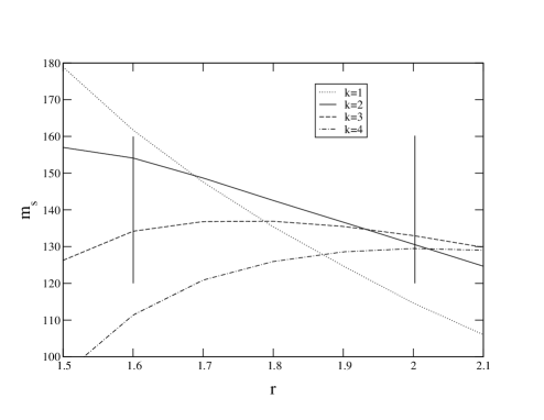
Figure 1: $m_{s}$ as function of $r$ for different $k$

4.2 The $R_{\tau}^{V}-{\mathcal{M}}^{\phi}$ sum rule

Here we consider a second sum rule that uses the difference of the strange vector current and the $\tau\ ud$ vector current which has been measured in [27]. The relevant moment reads

$${\mathcal{M}}^{1\phi}=\frac{1}{9}R^{V}_{\tau}-{\mathcal{M}}^{\phi}$$ (8)

where ${\mathcal{M}}^{\phi}$ is the moment from the strange quark current as discussed in the last section and $R^{V}_{\tau}$ is obtained from the $\tau$ vector current $j(x)=\bar{u}(x)\gamma_{\mu}d(x)$. The advantage of taking this difference is that the perturbative terms of the OPE drop out, and that the higher dimensional condensates partially cancel. Since the leading order contributions cancel the mass corrections become leading order. Effectively this sum rules substitutes theoretical uncertainties by better known experimental values. However, it has the drawback that the data are only available up to $M_{\tau}$ and so we can only apply a very limited sum rule window. As in the pure strange-vector current sum rule we use values of $k=2,3$ for the central value and $1\leq k\leq 4$ for the error estimate. Our central mass is slightly lower with $m_{s}(2\ \mbox{\rm GeV})=130\ \mbox{\rm MeV}$ with a similar error as before. However, since the sum rule window for $r$ is small we cannot check for the stability of the sum rule over a large range of values. Therefore we take the strange mass from section 4.1 as our central result and use the ${\mathcal{M}}^{1\phi}$ sum rule as a consistency check.

5 Conclusions

The finite energy sum rules provide a powerful method to determine the strange quark mass from the vector current and our preliminary result is

$$m_{s}(2~{}\mbox{\rm GeV})=139\pm 31~{}\mbox{\rm MeV}\,.$$ (9)

The theoretical contributions can be calculated either in FOPT or CIPT. Surprisingly, a large difference is found and we have commented on this topic in section 2.3. On the phenomenological side, we have included recent experimental results from CMD-2 [20]. Our result lies somewhat above other recent determinations [6, 7, 8, 9, 10]. Since this sum rule is independent of other methods, it provides an additional and complementary access to the strange quark mass.

References

- [1] M. Beneke and M. Neubert, arXiv:hep-ph/0308039.
- [2] A. Khodjamirian, T. Mannel and M. Melcher, arXiv:hep-ph/0308297.
- [3] M. A. Shifman, A. I. Vainshtein and V. I. Zakharov, Nucl. Phys. B 147 (1979) 385, 448.
- [4] L. J. Reinders, H. Rubinstein and S. Yazaki, Phys. Rept. 127 (1985) 1.
- [5] S. Narison, QCD spectral sum rules, World Sci. Lect. Notes Phys. 26 (1989) 1.
- [6] E. Gamiz, M. Jamin, A. Pich, J. Prades and F. Schwab, JHEP 0301 (2003) 060 [arXiv:hep-ph/0212230].
- [7] S. Chen, M. Davier, E. Gamiz, A. Hocker, A. Pich and J. Prades, Eur. Phys. J. C 22 (2001) 31 [arXiv:hep-ph/0105253].
- [8] P. Colangelo, F. De Fazio, G. Nardulli and N. Paver, Phys. Lett. B 408 (1997) 340 [arXiv:hep-ph/9704249].
- [9] M. Jamin, J. A. Oller and A. Pich, Eur. Phys. J. C 24 (2002) 237 [arXiv:hep-ph/0110194].
- [10] K. Maltman and J. Kambor, Phys. Rev. D 65 (2002) 074013 [arXiv:hep-ph/0108227].
- [11] J. G. Körner, F. Krajewski and A. A. Pivovarov, Eur. Phys. J. C 20 (2001) 259 [arXiv:hep-ph/0003165].
- [12] S. Narison, Phys. Lett. B 358 (1995) 113 [arXiv:hep-ph/9504333].
- [13] K. Maltman, Phys. Lett. B 428 (1998) 179 [arXiv:hep-ph/9804299].
- [14] K. Maltman and C. E. Wolfe, Phys. Rev. D 59 (1999) 096003 [arXiv:hep-ph/9810441].
- [15] S. Narison, Phys. Lett. B 466 (1999) 345 [arXiv:hep-ph/9905264].
- [16] Markus Eidemüller, Matthias Jamin and Felix Schwab, the strange quark mass from the vector current with finite energy sum rules, in preparation.
- [17] A. A. Pivovarov, Z. Phys. C 53 (1992) 461 [arXiv:hep-ph/0302003].
- [18] F. Le Diberder and A. Pich, Phys. Lett. B 286 (1992) 147.
- [19] A. Pich and J. Prades, JHEP 9806 (1998) 013 [arXiv:hep-ph/9804462].
- [20] R. R. Akhmetshin et al. [CMD-2 Collaboration], arXiv:hep-ex/0308008.
- [21] A. Pich and J. Prades, JHEP 9910 (1999) 004 [arXiv:hep-ph/9909244].
- [22] G. Grunberg, Phys. Rev. D 29 (1984) 2315.
- [23] P. M. Stevenson, Phys. Rev. D 23 (1981) 2916.
- [24] R. Barate et al. [ALEPH Collaboration], Eur. Phys. J. C 4 (1998) 409.
- [25] V. Cirigliano, E. Golowich and K. Maltman, Phys. Rev. D 68 (2003) 054013 [arXiv:hep-ph/0305118].
- [26] S. Eidelman and F. Jegerlehner, Z. Phys. C 67 (1995) 585 [arXiv:hep-ph/9502298].
- [27] R. Barate et al. [ALEPH Collaboration], Z. Phys. C 76 (1997) 15.