A Model for the Off-forward Structure Functions of the Pion

Abstract

We extend our model for the pion, which we used previously to calculate its diagonal structure function, to the off-forward case. The imaginary part of the off-forward $\gamma^{\star}\pi\rightarrow\gamma^{\star}\pi$ scattering amplitude is evaluated in the chiral limit ($m_{\pi}=0$) and related to the twist-two and twist-three generalised parton distributions ${H}$, ${H}^{3}$, $\tilde{H}^{3}$. Non-perturbative effects, linked to the size of the pion and still preserving gauge invariance, are included. Remarkable new relations between ${H}$, ${H}^{3}$ and $\tilde{H}^{3}$ are obtained and discussed.

, , , and

1 Introduction

Structure functions, which can be extracted from deep-inelastic experiments, are useful tools to understand the structure of hadrons. Even if their $Q^{2}$ evolution is consistent with perturbative QCD, they result mainly from non-perturbative effects that are still not calculable in the framework of QCD. This has led to phenomenological quark models embodying various non-perturbative aspects of QCD. These models can be used to depict the behaviour of the structure functions and to understand the connection between data and non-perturbative aspects of hadrons. There has been extensive work on diagonal distributions along these lines (see Refs [1]-[2] for the pion case). These distributions can be used as the initial condition for a DGLAP evolution, which is necessary before a comparison with data [3]. Such models can be applied to the off-diagonal case, for which generalised structure functions [4] can be linked [5] to generalised parton distributions (GPD’s).

One of the setbacks of phenomenological quark models suited to the description of the low-energy features of hadrons is that the underlying quark structure is obscured by the necessary introduction of regularisation procedures which result in non-negligible differences in the structure functions.

To avoid these complications, we investigated the diagonal structure functions in the case of a simple model for the pion [1], where the pion-quark-antiquark pseudoscalar coupling ($i\gamma^{5}g_{\pi q\bar{q}}$) yields the correct symmetry, while the non-perturbative aspects come from a momentum cut-off mimicking the size of the pion, but still preserving gauge invariance. This freed us from the question of what would be the detailed inner structure of the meson. In that calculation, owing to the introduction of such a cut-off, crossed diagrams for the pion-photon scattering appear as higher twists, leading twist structure functions can be identified, and a reduction of the momentum fraction carried by the quarks is observed. Of course, as the cut-off is relaxed to let the quarks behave freely, the momentum sum rule $\left<2x\right>=1$ is recovered at infinite $Q^{2}$. Having that tool at hand, we now turn to the investigation of the properties of off-diagonal parton distributions, which are likely to shed some light on parton correlations and which have therefore attracted much interest in recent years [6, 7, 8, 9, 10, 11].

In the following, we calculate the imaginary part of the off-forward photon-pion scattering amplitude, and of the structure functions $F_{1},\dots,\ F_{5}$, related to the five independent tensor structures in the scattering amplitude, and we discuss their behaviour. We relate them to vector and axial vector form factors and to the twist-two and twist-three generalised parton distributions (GPD’s) ${H}$, ${H}^{3}$ and $\tilde{H}^{3}$. We shall show that, within our model and in the high-$Q^{2}$ limit, the non-diagonal structure functions $F_{3}$ and $F_{4}$ are related to $F_{1}$, while $F_{5}$ happens to be a higher twist. These results lead to new relations for the GPD’s in the neutral pion case.

2 General tensorial structure of the $\gamma^{\star}\pi\rightarrow\gamma^{\star}\pi$ amplitude

2.1 External Kinematics

Let $p_{1}$ and $p_{2}$ be the momenta of the ingoing and outgoing pions, $q_{1}$ and $q_{2}$ those of the corresponding photons (see Fig. 1).

     

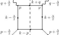
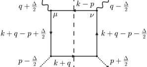
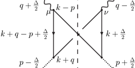
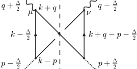
Figure 1: The simplest diagrams contributing to the imaginary part of the amplitude for the scattering $\gamma^{\star}\pi\rightarrow\gamma^{\star}\pi$. Upper (lower) diagrams are referred to as box (crossed) diagrams. Dashed lines represent the discontinuity of the amplitudes, i.e. their imaginary parts.

Defining $p=\frac{(p_{1}+p_{2})}{2}$, $q=\frac{(q_{1}+q_{2})}{2}$ and $\Delta=p_{2}-p_{1}$, one can then write the scattering amplitude as a function of the Lorentz invariants $t=\Delta^{2}$, $Q^{2}=-q^{2}$, $x=\frac{Q^{2}}{2p\cdot q}$ and $\xi=\frac{\Delta\cdot q}{2p\cdot q}$.

In the elastic limit, characterised by $(q+\frac{\Delta}{2})^{2}=(q-\frac{\Delta}{2})^{2}$, one has $\Delta\cdot q=0$ and thus $\xi=0$, while the diagonal limit ($\Delta=0$) is obtained for $\xi=0$ and $t=0$. We further recover the Bjorken variable $x=x_{B}$, where $x_{B}=-\frac{q_{1}^{2}}{2p_{1}\cdot q_{1}}$.

For Virtual Compton Scattering (VCS), for which the outgoing photon is on-shell, $\xi$ is related to $x$ through $\xi=-x\left(1-\frac{\Delta^{2}}{4Q^{2}}\right)$. Hence in the Deeply Virtual Compton Scattering (DVCS) limit, $t\ll Q^{2}$ and $\xi=-x$.

2.2 The structure functions $F_{i}$’s

The hadronic tensor is defined through

$$T_{\mu\nu}(q,p,\Delta)=i\!\int\!d^{4}r{\rm e}^{ir\cdot q}\left<p_{2}|Tj_{\mu}(r/2)j_{\nu}(-r/2)|p_{1}\right>.$$ (1)

There exist five independent kinematical structures in Eq. (1) that parametrise the photon-pion amplitude. Defining the projector ${\cal P}_{\mu\nu}=g_{\mu\nu}-\frac{q_{2\mu}q_{1\nu}}{q_{1}\cdot q_{2}}$ and making use of these five structures, we can rewrite $T_{\mu\nu}$ as follows:

$$T_{\mu\nu}(q,p,\Delta)=-{\cal P}_{\mu\sigma}g^{\sigma\tau}{\cal P}_{\tau\nu}F_{1}+\frac{{\cal P}_{\mu\sigma}p^{\sigma}p^{\tau}{\cal P}_{\tau\nu}}{p\cdot q}F_{2}$$

$$+\frac{{\cal P}_{\mu\sigma}(p^{\sigma}(\Delta^{\tau}-2\xi p^{\tau})+(\Delta^{\sigma}-2\xi p^{\sigma})p^{\tau}){\cal P}_{\tau\nu}}{2p\cdot q}F_{3}$$

$$+\frac{{\cal P}_{\mu\sigma}(p^{\sigma}(\Delta^{\tau}-2\xi p^{\tau})-(\Delta^{\sigma}-2\xi p^{\sigma})p^{\tau}){\cal P}_{\tau\nu}}{2p\cdot q}F_{4}$$

$$+{\cal P}_{\mu\sigma}(\Delta^{\sigma}-2\xi p^{\sigma})(\Delta^{\tau}-2\xi p^{\tau}){\cal P}_{\tau\nu}F_{5}.$$ (2)

Current conservation is ensured by means of the projector ${\cal P}_{\mu\nu}$. Our notation slightly differs from Ref. [5]: we have included a factor $1/m_{\pi}^{2}$ in the definition of $F_{5}$ in order to avoid divergences when the chiral limit is taken. Note that Bose symmetry requires $F_{1}$, $F_{2}$, $F_{4}$, $F_{5}$ to be even and $F_{3}$ to be odd in $\xi$.

3 The model

3.1 General description

We use the pion model introduced in our previous work [1], in which the $q\overline{q}\pi$ vertex is represented by the simplest pseudoscalar coupling. The Lagrangian includes massive pion and massive quark fields interacting through the pseudoscalar vertex, with an effective pion-quark coupling constant.

Considering an isospin triplet pion field $\vec{\pi}=(\pi^{+},\pi^{0},\pi^{-})$ interacting with quark fields $\psi$ the Lagrangian density reads

$${\mathcal{L}}_{int}=ig(\overline{\psi}\mbox{ $\vec{\tau}$}\gamma_{5}\psi).\mbox{ $\vec{\pi}$},$$ (3)

where $\vec{\tau}$ is the isospin vector operator.

Of course, if our pseudoscalar field is to represent real pions, we have to impose that the corresponding hadrons have a finite size. That we shall do through the use of a cut-off, as detailed below, the choice of which sets a constraint on the value of the quark-pion coupling constant [1].

We shall limit ourselves in this paper to the calculation of the imaginary part of the scattering amplitude, which allows a direct comparison with our previous work and which is sufficient to determine the GPD’s of neutral pions [5].

At the leading order in the loop expansion, four diagrams contribute. They are displayed in Fig. 1. Following the kinematics defined in section 2.1 and applying Feynman rules, it is straightforward to write down the analytical expression for the scattering amplitude. For a given set $\mu,\nu$ of the photon indices and with well-known conventions, the contribution of the first diagram (a) shown in Fig. 1 to the scattering amplitude reads

$${\cal M}^{\mu\nu}_{a}=3g^{2}(e_{u}^{2}+e_{d}^{2})\int{\rm d}^{4}k{\rm Tr}(\gamma^{5}((k\!\!\!/-p\!\!\!/)+m_{q})\gamma^{5}$$

$$\frac{k\!\!\!/+\frac{\Delta\!\!\!/}{2}+m_{q}}{(k+\frac{\Delta}{2})^{2}-m_{q}^{2}}\gamma^{\nu}((k\!\!\!/+q\!\!\!/)+m_{q})\gamma^{\mu}\frac{k\!\!\!/-\frac{\Delta\!\!\!/}{2}+m_{q}}{(k-\frac{\Delta}{2})^{2}-m_{q}^{2}}).$$ (4)

Expressions from the other three diagrams of Fig. 1 – the one with reverse loop-momentum and the two crossed diagrams – are similar and are not written down. Results below all pertain to the chiral limit $m_{\pi}=0$.

3.2 The implementation of the cut-off

A simple way to impose that the pion has a finite size is to require that the square of the relative four-momentum of the quarks inside the pion is limited to a maximum value $\Lambda^{2}$. Before writing this explicitly, let us give the details of the internal kinematics, i.e. the one involving the loop-momentum $k$. Let $\phi$ and $\theta$ be the spherical angles of $\vec{k}$ with respect to the $z$-axis taken as the direction of the incoming photon. Defining $k_{\rho}^{2}=|\vec{k}|^{2}$ and $\tau=k^{2}=k^{2}_{0}-k_{\rho}^{2}$, and using spherical coordinates, we write the element of integration as:

$$d^{4}k=dk_{0}dk_{\rho}k_{\rho}^{2}d(\cos\theta)d\phi,$$ (5)

or with the help of the variable $\tau$:

$$d^{4}k=dk_{0}\frac{k_{\rho}}{2}d\tau d(\cos\theta)d\phi.$$ (6)

According to Cutkosky rules, the imaginary part of the amplitude is obtained by putting the intermediate quark lines on shell. This is realised by the introduction of the two delta functions, $\delta\left((k+q)^{2}-m_{q}^{2}\right)$ and $\delta\left((k-p)^{2}-m_{q}^{2}\right)$.

Working out the delta functions, we obtain that:

$$\delta\left((k+q)^{2}-m_{q}^{2}\right)\delta\left((k-p)^{2}-m_{q}^{2}\right)=$$

$$\frac{1}{2k_{\rho}|\vec{q}|}\delta\left(\cos\theta-\cos\theta_{0}\right)\frac{1}{2\sqrt{s}}\delta\left(k_{0}-k^{\prime}_{0}\right)$$ (7)

with $\cos\theta_{0}=\frac{2k_{0}q_{0}-Q^{2}-m_{q}^{2}+\tau}{2k_{\rho}|\vec{q}|}$ and $k^{\prime}_{0}=\frac{Q^{2}+m_{\pi}-\frac{t}{4}}{2\sqrt{s}}$. Finally, the element of integration over the internal momentum, considering only the imaginary part of the amplitude, reads:

$$d^{4}k=d\tau d\phi\left.\frac{1}{8\sqrt{s}|\vec{q}|}\right|_{k_{0}=k^{\prime}_{0},\cos\theta=\cos\theta_{0}},$$ (8)

with $|\vec{q}|=\frac{1}{2x}\sqrt{\frac{4sx^{2}Q^{2}+(1-2x)^{2}Q^{4}}{s}}$. The boundary values of the integration domain on $\tau$ are obtained by solving $\cos\theta_{0}=\pm 1$.

Now we may look at the effect of the finite size of the pion on the integration procedure upon $k$. The relative four-momentum squared of the quarks inside the pion is given by

$$O_{1}^{\pm} = \left(2k-p\pm\frac{\Delta}{2}\right)^{2}$$ (9)

$$= 2\tau+2m_{q}^{2}-m_{\pi}^{2}+\frac{t}{2}\pm 2k\cdot\Delta,$$

for pion-quark vertices like the ones in diagram Fig. 1.(a), and by

$$O_{2}^{\pm}=\left(2k-p+2q\pm\frac{\Delta}{2}\right)^{2}$$ (10)

$$= -2\tau+6m_{q}^{2}-m_{\pi}^{2}+\frac{t}{2}-\frac{2Q^{2}}{x}\pm 2(k\cdot\Delta+\frac{\xi Q^{2}}{x}),$$

for vertices as in diagram Fig. 1.(b). Note that $k\cdot\Delta$ is a known function of the external variables as well as of $\theta$ and $\tau$. Generalising the procedure of [1], we require either $|O_{1}^{\pm}|<\Lambda^{2}$ or $|O_{2}^{\pm}|<\Lambda^{2}$ for all diagrams. Gauge invariance is preserved by the cut-off, since $|O_{i}^{\pm}|$ depend only upon the external variables of the $\gamma^{\star}\pi\to q\bar{q}$ process.

As the $O_{i}$’s and $\tau$ are always negative, we require one of the two following conditions:

$$\tau > \frac{-\Lambda^{2}}{2}+\frac{m_{\pi}^{2}}{2}-m_{q}^{2}-\frac{t}{4}+\left|k\cdot\Delta\right|,$$

$$\tau < \frac{\Lambda^{2}}{2}-\frac{m_{\pi}^{2}}{2}+3m_{q}^{2}+\frac{t}{4}-\frac{Q^{2}}{x}-\left|\frac{\xi Q^{2}}{x}+k\cdot\Delta\right|.$$ (11)

For $t$ small, $|O_{1}|$ and $|O_{2}|$ cannot be small simultaneously. The crossed diagrams have their main contribution for $O_{1}\simeq O_{2}$, and are thus suppressed by a power $\Lambda^{2}/Q^{2}$ when the cut-off is imposed. The box diagrams have a leading contribution for $|O_{1}|$ or $|O_{2}|$ small, and are not power suppressed by the cut-off.

It may be worth pointing out that the vertical propagators are more off-shell in DVCS than in DIS, hence one would expect DVCS to be better described by perturbation theory than DIS.

3.3 The coupling constant

In the diagonal case, we have determined the coupling constant $g=g_{\pi qq}$ by imposing that there are only two constituents in the pion. This sum rule constraints $F_{1}$ as follows [1]:

$$\int_{0}^{1}F_{1}(x)dx=\frac{5}{18}.$$ (12)

As $F_{1}/g^{2}$ is a priori a function of $Q^{2}$, the sum rule imposes that $g$ should be a function of $Q^{2}$. But at high enough $Q^{2}$, where the details of the non-perturbative interaction are less and less relevant, $F_{1}/g^{2}$ reaches its asymptotic shape when the cut-off procedure is applied, and we obtain a constant value for $g$. In Ref. [1], this asymptotic regime was reached for $Q^{2}$ as small as 2 GeV². In the following, we shall make use of these previously obtained values, which are functions of the cut-off $\Lambda$.

However in the DVCS case, an ambiguity may arise as one of the vertices has an external kinematics similar to a vanishing $Q^{2}$ DIS. This ambiguity is lifted if one notices that the pertinent quantities are not $q_{1}^{2}$ and $q_{2}^{2}$ separately but the factorisation scale, which may be taken as the square of their mean, $Q^{2}$. Thus in DVCS, although $q_{2}^{2}$ vanishes, $Q^{2}$ does not and we shall consider that $g$ is constant.

4 Results

4.1 General features

From the imaginary part of the total amplitude, the five structure functions $F_{i}$ can be obtained by a projection on the corresponding tensors. From now on, $F_{i}$ will stand for the imaginary part of these structure functions. In order to display their general features, we plot them in Fig. 2 first as functions of $x$ and $\xi$ for parameter values $m_{q}=0.3$ GeV and $\Lambda=0.75$ GeV, to ease the comparison with [1], and for $Q^{2}=10$ GeV² and $t=-0.1$ GeV². Let us notice that for any fixed value of $\xi$ not close to $\pm 1$, we recover for $F_{1}$ and $F_{2}$ the same behaviour as in the diagonal case. We checked indeed that the diagonal limit is recovered for $\xi=0$ and $t=0$. Let us notice also that the structure functions $F_{3}$, $F_{4}$, $F_{5}$ depend little on $\xi$ except when this variable is close to $\pm 1$.

Figure 2: Plot of the five structure functions as functions of $x$ ($\in[0,1]$)and $\xi$ ($\in[-1,1]$) with a cut-off $\Lambda=0.75$ GeV, at $Q^{2}=10$ GeV² and $t=-0.1$ GeV².

Let us turn now to DVCS. Fig. 3 displays the behaviour of $F_{1}$ for various values of $t$ with and without cut-off. In the presence of size effects, the value of $F_{1}$ gets significantly reduced, especially for small $x$, as $|t|$ increases, whereas that effect is much less noticeable without cut-off.

 

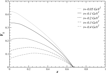
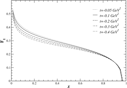
Figure 3: $F_{1}$ as a function of $x$ for various values of $t$ in the DVCS case with (a) and without (b) cut-off ($\Lambda=0.75$ GeV), at $Q^{2}=10$ GeV².

 

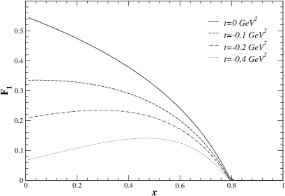
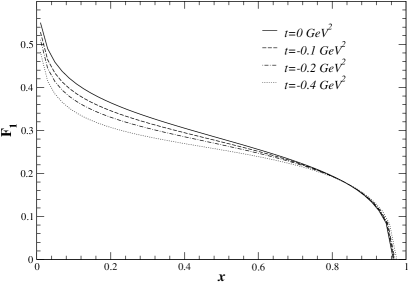
Figure 4: Evolution of $F_{1}$ (elastic case, $\xi=0$) for decreasing values of $t$ with (a) and without (b) cut-off, for $Q^{2}=10$ GeV².

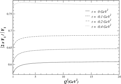
Figure 5: Mean value of $2x$ for the $F_{1}$ distribution in the elastic case ($\xi=0$) as a function of $Q^{2}$ and for various values of $t$.

In the elastic case (see Fig. 4), the same suppression at small $x$ is observed, especially when the cut-off is applied. In Fig. 5, we display the average value of $2x$ with respect to the $F_{1}$ distribution. The value of $\left<2x\right>$ increases when $|t|$ increases. The momentum fraction carried by the quarks and probed by the process thus increases with the momentum transfer.

 

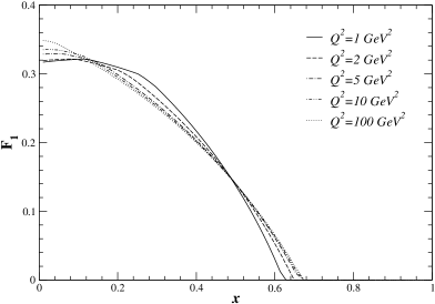
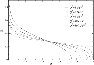
Figure 6: $F_{1}$ as a function of $x$ for $t=-0.1$ GeV² and for various values of $Q^{2}$ in the DVCS case with (a) and without (b) cut-off.

The effects of the variation of $Q^{2}$ are displayed in Fig. 6. As in the diagonal case [1], we can conclude that the details of the non-perturbative effects cease to matter for $Q^{2}$ greater than 2 GeV², that is significantly larger than $\Lambda^{2}$. On the other hand, when the cut-off is not applied, we see (Fig. 6 (b)) that $F_{1}$ evolves so slowly with $Q^{2}$ that the asymptotic state is not visible.

4.2 High-$Q^{2}$ limit: new relations

Having determined the 5 functions $F_{i}$’s in the context of our model, we shall now consider their behaviour at high $Q^{2}$. Expanding the ratios of $\frac{F_{2}}{F_{1}}$$,\frac{F_{3}}{F_{1}}$,$\frac{F_{4}}{F_{1}}$,$\frac{F_{5}}{F_{1}}$, we obtain the following asymptotic behaviour:

$$F_{2} = 2xF_{1}+{\cal O}(1/Q^{2}),$$ (13)

$$F_{3} = \frac{2x\xi}{\xi^{2}-1}F_{1}+{\cal O}(1/Q^{2}),$$ (14)

$$F_{4} = \frac{2x}{\xi^{2}-1}F_{1}+{\cal O}(1/Q^{2}),$$ (15)

$$F_{5} = {\cal O}(1/Q^{2}).$$ (16)

The fact that at leading order there are only three independent structure functions has been known for some time [5, 10]. However, we show here that they can all be obtained from $F_{1}$. The first relation is similar (at leading order in $1/Q^{2}$ and with the replacement of $x$ by $x_{B}$) to the Callan-Gross relation between the diagonal structure functions $F_{1}$ and $F_{2}$, valid for spin one-half constituents in general. Except for $F_{5}$, which is small at large $Q^{2}$, these relations show that $F_{2}$, $F_{3}$ and $F_{4}$ are simply related to $F_{1}$ at leading order. These relations clearly display and therefore confirm the symmetries of these functions. Combining Eqs. (14) and (15), we have, at leading order,

$$F_{3}=\xi F_{4},$$ (17)

which confirms that $F_{3}$ is an odd function of $\xi$, while $F_{4}$ is even.

The simple relations between the $F_{i}$’s (at leading order) constitute a remarkable result of our model. Furthermore, we checked that the term ${\cal O}(1/Q^{2})$ in Eq. (13) is numerically quite small, even for moderate $Q^{2}$. One may wonder whether these results are typical of our model or more general.

5 Linking the $F_{i}$’s to ${H}$, ${H}^{3}$, and $\tilde{H}^{3}$

Figure 7: A comparison of the values of $H_{3}$ and $\tilde{H}_{3}$ obtained in our model (left) with those calculated in the Wandzura-Wilczek approximation, using the value of $H$ from our model (right), for $Q^{2}=10$ GeV².

Having at hand the five functions $F_{i}$’s that parametrise the amplitude for $\gamma^{\star}\pi\to\gamma^{\star}\pi$, we would like to link them to the off-forward parton distribution functions or to the generalised parton distributions. For this purpose, we make use of a tensorial expression coming from the twist-three analysis of the process, which singles out the twist-two ${\cal H}$ and the twist-three ${\cal H}^{3},\tilde{\cal H}^{3}$ form factors. Following Ref. [5], we write:

$$T_{\mu\nu}(q,p,\Delta)= - {\cal P}_{\sigma\mu}g^{\sigma\tau}{\cal P}_{\nu\tau}\frac{q\cdot V_{1}}{2p\cdot q}$$ (18)

$$+ \left({\cal P}_{\sigma\mu}p^{\sigma}{\cal P}_{\nu\rho}+{\cal P}_{\rho\mu}p^{\sigma}{\cal P}_{\nu\sigma}\right)\frac{V_{2}^{\rho}}{p\cdot q}$$

$$- {\cal P}_{\sigma\mu}i\epsilon^{\sigma\tau q\rho}{\cal P}_{\nu\tau}\frac{A_{1\,\rho}}{2p\cdot q}.$$

where the $V_{i}$’s and $A_{1}$ read

$$V_{1\,\rho} = 2p_{\rho}{\cal H}+(\Delta_{\rho}-2\xi p_{\rho}){\cal H}^{3}+\mbox{twist 4},$$ (19)

$$A_{1\,\rho} = \frac{i\epsilon_{\rho\Delta pq}}{p\cdot q}\;{\tilde{\cal H}}^{3},$$ (20)

$$V_{2\,\rho} = xV_{1\,\rho}-\frac{x}{2}\frac{p_{\rho}}{p\cdot q}q\cdot V_{1}+\frac{i}{4}\frac{\epsilon_{\rho\sigma\Delta q}}{p\cdot q}A_{1}^{\sigma}+\mbox{twist 4}.$$

In Ref. [5], gauge invariance of Eq. (18) beyond the twist-three accuracy was in fact restored by hand, contrarily to the present calculation for which the amplitude is explicitly gauge invariant.

To relate the $F_{i}$’s to the $\cal H$’s, we project the amplitude (18) onto the five projectors contained in Eq. (2.2) and identify the results with the $F_{i}$’s. Note that, in the neutral pion case, the imaginary part of the form factors $\cal H$ directly gives the GPD’s $H$, $H^{3}$ and $\tilde{H}^{3}$ up to a factor $2\pi$. As we have kept the off-shellnesses of the photons arbitrary, we in fact can relate the imaginary parts of $F_{i}$ to the GPD’s for arbitrary $x$ and $\xi$:

$${1\over 2\pi}F_{1} = {H},$$ (22)

$${1\over 2\pi}F_{2} = 2x{H}+{\cal O}(\frac{1}{Q^{2}}),$$ (23)

$${1\over 2\pi}F_{3} = \frac{2x}{x^{2}-\xi^{2}}\left({H}^{3}x^{2}+\tilde{H}^{3}\xi x-{H}\xi\right)+{\cal O}(\frac{1}{Q^{2}}),$$ (24)

$${1\over 2\pi}F_{4} = \frac{2x}{x^{2}-\xi^{2}}\left({H}^{3}\xi x+\tilde{H}^{3}x^{2}-{H}x\right)+{\cal O}(\frac{1}{Q^{2}}),$$ (25)

$${1\over 2\pi}F_{5} = {\cal O}(\frac{1}{Q^{2}}).$$ (26)

Replacing the $F_{i}$’s by the expressions (13-16), we can write

$$\tilde{H}^{3}=\frac{(x-1)}{x(\xi^{2}-1)}H+{\cal O}(\frac{1}{Q^{2}}),$$ (27)

and

$${H}^{3} = \frac{(x-1)\xi}{x(\xi^{2}-1)}H+{\cal O}(\frac{1}{Q^{2}})=\xi\tilde{H}^{3}+{\cal O}(\frac{1}{Q^{2}}).$$ (28)

As $F_{1}$ to $F_{4}$ can be written in term of only one of them, e.g. $F_{1}$, it is not surprising that ${H}^{3}$ and ${\tilde{H}}^{3}$ are simply related to ${H}$. Note that polynomiality of the Mellin moments of $H$, $H^{3}$ and $\tilde{H}^{3}$, together with Eqs. (27) and (28), imply that $H$ must be a polynomial $P_{H}$ multiplying $\xi^{2}-1$. The fact that, as can be seen from Fig. 7, $\tilde{H}_{3}$ is almost independent of $\xi$ shows that $P_{H}$ is very close to a constant.

To convince ourselves that relations (27) and (28) are new, we have compared them to the Wandzura-Wilczek approximation [12], given in the pion case in [5, 13]. First of all, it is well-known that these relations are discontinuous at $\xi=\pm x$, which is not the case for (27) and (28). Furthermore, we show in Fig. 7 the results of the Wandzura-Wilczek approximation compared with our results. We see that the two are numerically very different. Hence the relations (27) and (28), derived in an explicitly gauge-invariant model, do not come from ”kinematical” twist corrections, but emerge from the dynamics of the spectator quark propagator and from finite-size effects.

6 Discussion and conclusion

We have extended our previous model for the pion to investigate the off-diagonal structure functions for this particular case. The introduction of a cut-off allows the crossed diagrams to behave as higher-twists and to relate the imaginary part of the forward amplitude with quark GPD’s.

We used the formalism of Ref. [5] in order to decompose the amplitude along the relevant Lorentz tensors, to define five structure functions $F_{i}$, and to relate the latter to the GPD’s ${H}$, ${H}^{3}$ and $\tilde{H}^{3}$ introduced in the twist analysis. We have found that our results in the forward case are qualitatively preserved when departing from the forward limit.

Our investigation yields new results. In particular, we singled out new relations, which link the $F_{i}$’s in a simple manner at leading order in $1/Q^{2}$. More intriguing, we found that the twist-three structure functions are simply related to ${H}$ by relations that differ from the Wandzura-Wilczek approximation.

Although these relations are derived in the context of our simple model, it is possible that they can be extended to a more general case.

References

- [1] F. Bissey, J. R. Cudell, J. Cugnon, M. Jaminon, J. P. Lansberg and P. Stassart, Phys. Lett. B 547 (2002) 210 [arXiv:hep-ph/0207107]; J. P. Lansberg, F. Bissey, J. R. Cudell, J. Cugnon, M. Jaminon and P. Stassart, AIP Conf. Proc. 660 (2003) 339 [arXiv:hep-ph/0211450].
- [2] T. Shigetani, K. Suzuki and H. Toki, Phys. Lett. B 308 (1993) 383 [arXiv:hep-ph/9402286]; R. M. Davidson and E. Ruiz Arriola, Phys. Lett. B 348 (1995) 163; H. Weigel, E. Ruiz Arriola and L. P. Gamberg, Nucl. Phys. B 560 (1999) 383 [arXiv:hep-ph/9905329]; E. Ruiz Arriola, Acta Phys. Polon. B 33 (2002) 4443 [arXiv:hep-ph/0210007]; P. Maris and C. D. Roberts, Int. J. Mod. Phys. E 12 (2003) 297 [arXiv:nucl-th/0301049]; W. Detmold, W. Melnitchouk and A. W. Thomas, Phys. Rev. D 68 (2003) 034025 [arXiv:hep-lat/0303015].
- [3] M. Glück, E. Reya and I. Schienbein, Eur. Phys. J. C 10 (1999) 313 [arXiv:hep-ph/9903288].
- [4] D. Müller, D. Robaschik, B. Geyer, F. M. Dittes and J. Hořejši, Fortsch. Phys. 42 (1994) 101 [arXiv:hep-ph/9812448].
- [5] A. V. Belitsky, D. Müller, A. Kirchner and A. Schäfer, Phys. Rev. D 64 (2001) 116002 [arXiv:hep-ph/0011314].
- [6] X. D. Ji, Phys. Rev. Lett. 78 (1997) 610 [arXiv:hep-ph/9603249]; Phys. Rev. D 55 (1997) 7114 [arXiv:hep-ph/9609381].
- [7] A. V. Radyushkin, Phys. Lett. B 380 (1996) 417 [arXiv:hep-ph/9604317]; Phys. Rev. D 56 (1997) 5524 [arXiv:hep-ph/9704207].
- [8] J. C. Collins, L. Frankfurt and M. Strikman, Phys. Rev. D 56 (1997) 2982 [arXiv:hep-ph/9611433].
- [9] P. A. Guichon and M. Vanderhaeghen, Prog. Part. Nucl. Phys. 41 (1998) 125 [arXiv:hep-ph/9806305]; K. Goeke, M. V. Polyakov and M. Vanderhaeghen, Prog. Part. Nucl. Phys. 47 (2001) 401 [arXiv:hep-ph/0106012]; M. Diehl, Phys. Rept. 388 (2003) 41 [arXiv:hep-ph/0307382].
- [10] A. V. Radyushkin and C. Weiss, Phys. Rev. D 63 (2001) 114012 [arXiv:hep-ph/0010296]; Phys. Lett. B 493 (2000) 332 [arXiv:hep-ph/0008214].
- [11] W. Broniowski and E. Ruiz Arriola, arXiv:hep-ph/0307198; S. Dalley, Phys. Lett. B 570 (2003) 191 [arXiv:hep-ph/0306121]; L. Theussl, S. Noguera and V. Vento, arXiv:nucl-th/0211036; A. E. Dorokhov and L. Tomio, Phys. Rev. D 62 (2000) 014016 [arXiv:hep-ph/9803329]; I. V. Anikin, A. E. Dorokhov, A. E. Maksimov, L. Tomio and V. Vento, Nucl. Phys. A 678 (2000) 175 [arXiv:hep-ph/9905332];
- [12] S. Wandzura and F. Wilczek, Phys. Lett. B 72 (1977) 195.
- [13] N. Kivel, M. V. Polyakov, A. Schäfer and O. V. Teryaev, Phys. Lett. B 497 (2001) 73 [arXiv:hep-ph/0007315]. Note that the definitions of and differ by a factor from those of [5] which we follow.