Systematics of quark–antiquark states: where are the lightest glueballs?

Abstract

The analysis of the experimental data of Crystal Barrel Collaboration on the $p\bar{p}$ annihilation in flight with the production of mesons in the final state resulted in a discovery of a large number of mesons over the region 1900–2400 MeV, thus allowing us to systematize quark-antiquark states in the $(n,M^{2})$ and $(J,M^{2})$ planes, where $n$ and $J$ are radial quantum number and spin of the meson with the mass $M$. The data point to meson trajectories in these planes being approximately linear, with a universal slope. Basing on these data and results of the recent K-matrix analysis a nonet classification is performed. In the scalar-isoscalar sector, the broad resonance state $f_{0}(1200-1600)$ is superfluous for the $q\bar{q}$ classification, i.e. it is an exotic state. The ratios of coupling constants for the transitions $f_{0}\to\pi\pi,K\bar{K},\eta\eta,\eta\eta^{\prime}$ point to the gluonium nature of the broad state $f_{0}(1200-1600)$. The problem of the location of the lightest pseudoscalar glueball is also discussed.

 
The search for exotic mesons should be based on the classification of $q\bar{q}$-states. Exotic mesons are those which are superfluous for the $q\bar{q}$ systematics. The quark–antiquark systematics means:
(i) classification of $q\bar{q}$ states as states located on the $(n,M^{2})$ and $(J,M^{2})$ trajectories, and
(ii) determination of the quark–gluonium content of states from the analysis of the decay coupling constants, namely, hadronic and radiative decay couplings as well as weak ones.

For the hadronic decay coupling constants, the most reliable information comes from the $K$-matrix analysis. In addition, the $K$-matrix analysis allows us to study bare states (the states before the onset of the decay processes).  

1.Systematics of the $q\bar{q}$-states on the $(n,M^{2})$ and $(J,M^{2})$ planes.
The analysis of experimental data on the $p\bar{p}$ annihilation in flight with the production of mesons in the final state resulted in a discovery of the large number of mesons over the region 1900–2400 MeV [1]. This allowed us to systematize quark–antiquark states on the $(n,M^{2})$ and $(J,M^{2})$ planes. The data point to almost the linear meson trajectories on these planes, with a universal slope [2].

In Fig. 1, one can see the $(n,M^{2})$ trajectories for the $(I=1)$ states, which are drown for the $a_{1}$- and $a_{3}$-mesons (Fig. 1a), $\pi$-, $\pi_{2}$- and $\pi_{4}$-mesons (Fig. 1b), $b_{1}$- and $b_{3}$-mesons (Fig. 1c). All these trajectories reveal linear behaviour, such as

$$M^{2}=M_{0}^{2}+\mu^{2}(n-1),$$

with $\mu^{2}\simeq 1.2$ GeV²; $M_{0}$ is the mass of the ground (basic) state, $n=1$. The pion, being beyond the trajectory, is an exception, that is not a surprise, for the pion is a special particle in certain respect. In the classification, all these mesons should be treated as $q\bar{q}$-states. Using the spectroscopy notations for $q\bar{q}$-states, ${}^{2S+1}L_{J}$ where $S$ is the quark spin and $L$ is their orbital momentum, we assign the trajectories to mesons as follows:
 
$a_{1}(1230)\,{\rm trajectory}$: $n^{3}P_{1}q\bar{q}$-states, $a_{3}(2030)\,{\rm trajectory}$: $n^{3}F_{3}q\bar{q}$-states;
  $\pi(140)\,{\rm trajectory}$: $n^{1}S_{0}q\bar{q}$-states, $\pi_{2}(1670)\,{\rm trajectory}$: $n^{1}D_{2}q\bar{q}$-states, $\pi_{4}(2250)\,{\rm trajectory}$: $n^{1}G_{4}q\bar{q}$-states;
  $b_{1}(1235)\,{\rm trajectory}$: $n^{1}P_{1}q\bar{q}$-states, $b_{3}(2020)\,{\rm trajectory}$: $n^{1}F_{3}q\bar{q}$-states.
 
In Fig. 1c the state $b_{1}(1640)$ is shown which was not discovered in the experiment but is predicted by trajectories: the states we predict are denoted by open circles.

The trajectories $\rho,\rho_{3},a_{0},a_{2},a_{4}$ demonstrate linear behaviour as well. The $\rho$-trajectories are shown in Fig. 2a:
 
$\rho(770)$ trajectory: dominantly $n^{3}S_{1}\,q\bar{q}(L=0)$,     $\rho(1700)$ trajectory: dominantly $n^{3}D_{1}\;q\bar{q}(L=4)$.
 
The states ${}^{3}S_{1}\;q\bar{q}$ and ${}^{3}D_{1}\;q\bar{q}$ may mix with each other but considerable mass splitting of the $\rho(770)$ and $\rho(1700)$ states tells us that the mixing is not large. The $\rho_{3}$ and $a_{0}$, $a_{2}$, $a_{4}$ trajectories are shown in Figs. 2b and 2c:
 
$\rho_{3}(1690)$ trajectory: dominantly $n^{3}D_{3}\;q\bar{q}(L=2)$,     $\rho_{3}(2260)$ trajectory: dominantly $n^{3}G_{3}\;q\bar{q}(L=4)$,
$a_{0}(980)$ trajectory: $n^{3}P_{0}\;q\bar{q}(L=1)$,     $a_{2}(1320)$ trajectory: dominantly $n^{3}P_{2}\;q\bar{q}(L=1)$,
$a_{2}(2030)$ trajectory: dominantly $n^{3}F_{2}\;q\bar{q}(L=3)$,     $a_{4}(2005)$ trajectory: dominantly $n^{3}F_{4}\;q\bar{q}(L=3)$.

FIG. 1.: The (I=1)-mesons on the $(n,M^{2})$ planes: $\pi,a_{1},a_{3},b_{1},b_{3}$ rajectories

FIG. 2.: The (I=1)-mesons on the $(n,M^{2})$ planes: the $\rho,\rho_{3},a_{0},a_{2}$ trajectories

FIG. 3.: The (I=0)-states on the $(n,M^{2})$ planes: $f_{0},f_{2},\omega$ trajectories

The $a_{0}(980)$-resonance, which sometimes is discussed as a non-$q\bar{q}$ state, lays on the $q\bar{q}$-trajectory, that is an argument in favour of its quark–antiquark origin.

The figures 3 and 4 for the $I=0$ states confirm the linearity of trajectories on the $(n,M^{2})$-planes, with a universal slope $\mu^{2}\simeq 1.2-1.3$ GeV². In this sector, we face a doubling of trajectories due to the existence of two flavour states $n\bar{n}=(u\bar{u}+d\bar{d})/\sqrt{2}$ and $s\bar{s}$.

In Fig. 3, one can see the $f_{2}(1285)$ and $f_{2}(1525)$ trajectories, which are dominantly the ${}^{3}P_{2}\;(n\bar{n}+s\bar{s})$ states, and $f_{2}(2020)$ and $f_{4}(2020)$ ones, which are dominantly ${}^{3}F_{2}\;(n\bar{n}+s\bar{s})$ and ${}^{3}F_{4}\;(n\bar{n}+s\bar{s})$, correspondingly. Figure 3b demonstrates $f_{0}(980)$ and $f_{0}(1300)$ trajectories (${}^{3}P_{0}\;(n\bar{n}+s\bar{s})$ states), while figure 3c shows the trajectories $\omega(780)$, $\phi(1020)$ (dominantly ${}^{3}S_{1}\;(n\bar{n}+s\bar{s})$) and $\omega(1640)$ (dominantly ${}^{3}D_{1}\;(n\bar{n}+s\bar{s})$).

FIG. 4.: The (I=0)-states on the $(n,M^{2})$ planes: $\omega_{3},h_{1},\eta$ trajectories

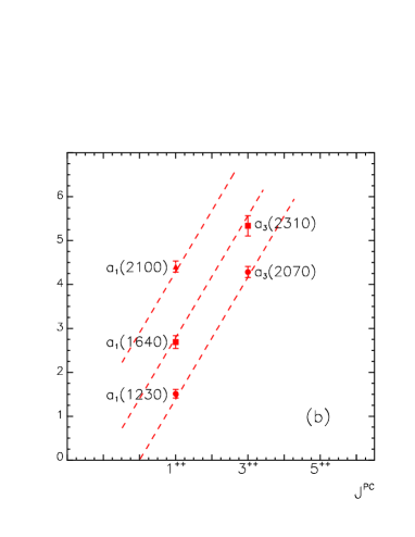
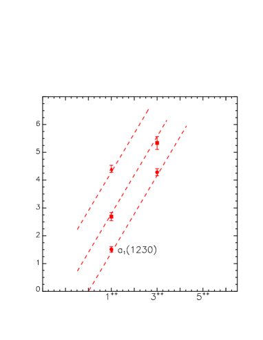
FIG. 5.: The $\pi$ and $a_{1}$ trajectories on the $(J,M^{2})$ plane.

Let me stress that $f_{0}(980)$, $f_{0}(1300)$ (the latter denoted as $f_{0}(1370)$ in the compilation [4]), $f_{0}(1500)$, $f_{0}(1750)$, which are sometimes discussed as candidates to exotics, lay quite comfortably on the linear $q\bar{q}$ trajectories. The K-matrix analysis [5] gives us one more state in the $(IJ^{PC}=00^{++})$-sector, that is, a broad resonance $f_{0}(1200-1600)$: just this state may be considered as exotics, a descendant of the lightest scalar glueball. It is discussed in the next section. The light $\sigma$, if it exists, is also beyond the $q\bar{q}$ trajectories being in this way a candidate for exotics as well.

In Figs. 4a,b,c, one can see trajectoties as follows: $\omega_{3},\;\phi_{3}$ (dominantely ${}^{3}D_{3}\;q\bar{q}$), $h_{1}$ (${}^{1}P_{1}\;q\bar{q}$), $\eta$ (${}^{1}S_{0}\;q\bar{q}$) and $\eta_{2}$ (${}^{1}D_{2}\;q\bar{q}$). Let me emphasize that the situation in the $0^{-+}$ sector is more complicated than it is seen from Fig. 4c. On the one hand, the states $\eta(1440)$ and $\eta(1295)$ lay good enough on the linear $(n,M^{2})$ trajectory. On the other hand, experimental indications for $\eta(1295)$ are not convincing, and the resonance $\eta(1440)$ reveals itself in different reactions

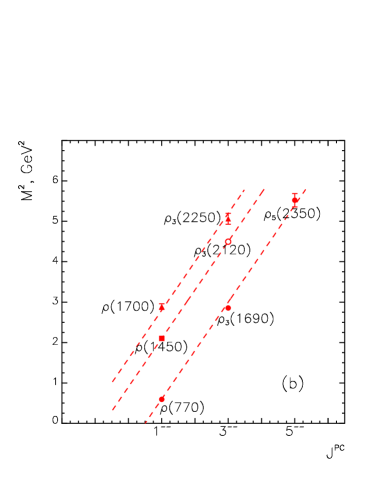
FIG. 6.: The $\rho$ and $a_{2}$ trajectories on the $(J,M^{2})$ plane.

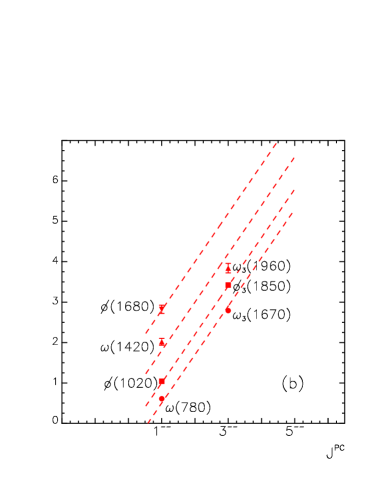
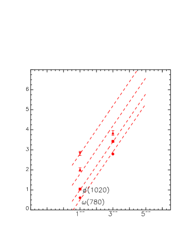
FIG. 7.: The $f_{2}$ and $\omega$ trajectories on the $(J,M^{2})$ plane.

with different masses: at 1390–1430 MeV in the $\eta\pi\pi$ and $a_{0}(980)\pi\to K\bar{K}\pi$ modes, while in the $K^{*}(890)\bar{K}$ mode at 1460–1500 MeV. Besides, in the reaction $J/\psi\to\gamma\eta(1440)$, the resonance $\eta(1440)$ is produced with a large background, that may tell us about the existence of a broad state at 1400–1700 MeV. Linear trajectories in the $0^{-+}$ sector predict two $q\bar{q}$ states in the neighbouring region, namely, $\eta(1700)$ and $\eta(1820)$, but these resonance were not seen till now, because, with available data this mass region is difficult for the study.

Now let us discuss the location of mesons on the $(J,M^{2})$-planes. The pion and $a_{1}$ trajectories are shown in Fig. 5a,b together with their daughter ones. The trajectories for different parities are degenerate — this fact is illustrated by Fig. 5c, where the combined presentation of $\pi$ and $a_{1}$ trajectories is given.

The $(J,M^{2})$ trajectories for $\rho$ and $a_{2}$ depicted in Fig. 6 provide us unambigous information on the $a_{0}(980)$ resonance. One can clearly see that $a_{0}(980)$ lays on the linear daughter trajectory — this is obvious from their combined presentation in Fig. 6c. Supposing that $a_{0}(980)$ is non-$q\bar{q}$ meson, one should expect another $a_{0}$ state, dominantly $q\bar{q}$, around 1 GeV. However, additional $a_{0}$ state is definitely excluded by the experimental data.

The $(J,M^{2})$ trajectories for the $f_{2}$ and $\omega$ resonances as well as for their daughter ones are shown in Fig. 7, and the combined presentation of Fig. 7c demonstrates the $f_{0}(980)$ resonance laying on the daughter $q\bar{q}$ trajectory.

At last, figure 8 shows us the trajectories for the $K$-meson sector, the kaons with positive and negative parities lay on the degenerate trajectories. The $\kappa$ meson discussed as a plausible $0^{+}$ state with the mass $\sim 900$ MeV does not belong to linear trajectory, so it should be considered as an exotic state.

Summing up the results of meson systematization on the $(n,M^{2})$ and $(J,M^{2})$ trajectories, one can state that the resonances $f_{0}(980),f_{0}(1300)$ ($f_{0}(1370)$ in [4]),$f_{0}(1500)$ and $f_{0}(1750)$ ($f_{0}(1710)$ in [4]) are located on quark–antiquark trajectories. They originate from the standard quark–antiquark states.

Now we can assign mesons to the flavour multiplets (see Tables 1, 2 for the multiplets with $n=1,2,3,4$). The interrogation sign marks the states, which were not discovered by the experiment but are predicted by linear $(n,M^{2})$ and $(J,M^{2})$ trajectories. The empty places are left for the states, which were not discovered and cannot be predicted.

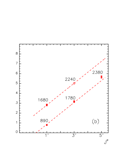
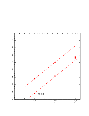
FIG. 8.: Trajectories on the $(J,M^{2})$ plane, $K$-meson sector.

One may conclude that there are extra $00^{++}$ states with respect to the $q\bar{q}$ systematics on the $(n,M^{2})$ and $(J,M^{2})$ trajectories:
1) the broad state $f_{0}(1200-1600)$ (it follows from the $K$-matrix analysis that it is the descendant of the glueball),
2) the light $\sigma$-meson, $f_{0}(300-500)$ (if it exists),
3) $\kappa$-meson, $K_{0}(700-900)$ (if it exists).

In the pseudoscalar-isoscalar sector $(IJ^{PC}=00^{-+})$, the situation in the mass region 1400-1800 MeV is rather uncertain, and one cannot exclude the states existing here, which are superfluous for the $q\bar{q}$ trajectories.

 

2. The $K$-matrix analysis of the ($IJ^{PC}=00^{++}$)-wave.
The trajectory assignment does not specify the content of the state. Each meson/resonance is a mixture of different components, and their wave functions are the Fock columns. For example, $a_{0}$ and $f_{0}$ may be considered as:

$a_{0}=\left(\begin{array}[]{c}q\bar{q}\\ qq\bar{q}\bar{q}\\ \eta\pi,K\bar{K},...\end{array}\right),$ $f_{0}=\left(\begin{array}[]{c}q\bar{q}\\ qq\bar{q}\bar{q}\\ \pi\pi,K\bar{K},\eta\eta,...\\ gg\end{array}\right)\,.$

In bare states, determined by the $K$-matrix analysis, the long-range hadronic components are excluded that makes possible more reliable determination of the quark-antiquark and gluonium ($gg$) components.

In the $K$-matrix analysis the partial wave amplitude reads:

$\widehat{A}(s)\ =\ \widehat{K}(s)\left[1-i\hat{\rho}\widehat{K}(s)\right]^{-1},$ $\widehat{K}=\left|\begin{array}[]{c}K_{11},K_{12},...\\ K_{21},K_{22},...\\ ...\\ \end{array}\right|,$ $\widehat{\rho}=\left|\begin{array}[]{c}\rho_{1},0,...\\ 0\;\;\;,\rho_{2},...\\ ...\\ \end{array}\right|\,.$

For the $00^{++}$ wave, which was analysed in [5], the following five channels were taken into account: $1=\pi\pi$, $2=K\bar{K}$,

$3=\eta\eta$, $4=\eta\eta^{\prime}$, $5=\pi\pi\pi\pi$, with the two-particle phase spaces determined as

$$\rho_{\pi\pi}=\sqrt{\frac{s-4m_{\pi}^{2}}{s}},\quad\rho_{KK}=\sqrt{\frac{s-4m_{K}^{2}}{s}},\quad...$$

while $\rho_{\pi\pi\pi\pi}$ was considerd as either two-$\sigma$ or two-$\rho$ phase space factor.

The fitting parameters are the $K$-matrix elements, which are represented as the sums of pole terms, $g^{(n)}_{a}g^{(n)}_{b}/(\mu^{2}_{n}-s)$, and a smooth $s$-dependent term $f_{ab}(s)$:

$$K_{ab}\ =\ \sum\limits_{n}\frac{g^{(n)}_{a}g^{(n)}_{b}}{\mu^{2}_{n}-s}+f_{ab}(s)\ ,$$

$M_{n}$ being the masses of bare states and $g_{a}$, $g_{b}$ their couplings.

The combined $K$-matrix analyses of the spectra have been performed for the mass interval $280\leq M\leq 1950$ MeV by including the following final states:

$$I=0: \quad\pi\pi,\;\eta\eta,\;K\bar{K},\;\eta\eta^{\prime},\;\pi\pi\pi\pi\;(\rho\rho,\;\sigma\sigma)\;\cite[cite]{[\@@bibref{Number}{EPJA}{}{}]},$$ (1)

$$I=1: \quad\pi\eta,\;K\bar{K}\;\cite[cite]{[\@@bibref{Number}{UFN}{}{}]},$$ (2)

$$I=\frac{1}{2}: \quad K\pi;\;\cite[cite]{[\@@bibref{Number}{Alex}{}{}]}.$$ (3)

Note that these combined $K$-matrix analyses have their predecessors published in [8]. The necessity of a combined analysis owes to the existence of large interference effects ”resonance–background” as well as the effects associated with the resonance overlapping. In a situation of such a type, only a combined fitting to a large number of reactions allows one to expect reliable results.

Previous analysis [6] carried out in 1997–1998 was based on the experimental data as follows:
(1) GAMS data on the $S$-wave two-meson production in the reactions $\pi p\to\pi^{0}\pi^{0}n$, $\eta\eta n$ and $\eta\eta^{\prime}n$ at small nucleon momenta transferred, $|t|<0.2$ (GeV/$c$)² [9, 10];
(2) GAMS data on the $\pi\pi$ $S$-wave production in the reaction $\pi p\to\pi^{0}\pi^{0}n$ at large momentum transfers squared, $0.30<|t|<1.0$ (GeV/$c$)² [9];
(3) BNL data on the reaction $\pi^{-}p\to K\bar{K}n$ [11];
(4) CERN-Münich data on $\pi^{+}\pi^{-}\to\pi^{+}\pi^{-}$ [12];
(5) Crystal Barrel data on $p\bar{p}$ (at rest, from liquid $H_{2}$)$\to\pi^{0}\pi^{0}\pi^{0}$, $\pi^{0}\pi^{0}\eta$, $\pi^{0}\eta\eta$ [13, 14].

Now the experimental basis has much broadened, and additional samples of data are included into the analysis [5] of the $00^{++}$ wave as follows:
(6) Crystal Barrel data on proton-antiproton annihilation in gas: $p\bar{p}$ (at rest, from gaseous $H_{2}$) $\to\pi^{0}\pi^{0}\pi^{0}$, $\pi^{0}\pi^{0}\eta$ [15].

One should keep in mind that in liquid hydrogen the $p\bar{p}$ annihilation is going dominantly from the $S$-wave state, while in gas there is a considerable admixture of the $P$-wave, thus giving us an opportunity to analyse the three-meson Dalitz plots in more detail.
(7) Crystal Barrel data on proton-antiproton annihilation in liquid: $p\bar{p}$ (at rest, from liquid $H_{2}$)$\to\pi^{+}\pi^{-}\pi^{0}$, $K^{+}K^{-}\pi^{0}$, $K_{S}K_{S}\pi^{0}$, $K^{+}K_{S}\pi^{-}$ [15];
(8) Crystal Barrel data on neutron-antiproton annihilation in liquid deuterium: $n\bar{p}$(at rest, from liquid $D_{2}$)$\to\pi^{0}\pi^{0}\pi^{-}$, $\pi^{-}\pi^{-}\pi^{+}$, $K_{S}K^{-}\pi^{0}$, $K_{S}K_{S}\pi^{-}$ [15].

These data allowed us to perform more confident study of the two-kaon channels as compared to what had been done before. This is important for the conclusion about the quark-gluon content of scalar–isoscalar $f_{0}$-mesons under investigation.
(9) E852 Collaboration data on the $\pi\pi$ $S$-wave production in the reaction $\pi^{-}p\to\pi^{0}\pi^{0}n$ at the nucleon momentum transfers squared $0<|t|<1.5\;({\rm GeV/c})^{2}$ [16].

Experimental data of the E852 Collaboration on the reaction $\pi^{-}p\to\pi^{0}\pi^{0}n$ at $p_{lab}=18$ GeV/c [16] together with the GAMS data on the reaction $\pi^{-}p\to\pi^{0}\pi^{0}n$ at $p_{lab}=38$ GeV/c [9] give us a solid ground for the study of the resonances $f_{0}(980)$ and $f_{0}(1300)$, for at large momenta transferred to the nucleon, $|t|\sim(0.5-1.5)$ (GeV/c)², the production of resonances is accompanied by a small background, thus allowing us to fix reliably their masses and widths.

The most important ingredients of the new analysis [5] are:
(i) the study of $K\bar{K}$-spectra that led to the determination of the flavour-octet and flavour-singlet components;
(ii) the study of $f_{0}(1300)$ produced without background: $\pi N\to\pi\pi N$ at large $|t|$.

Figure 9 taken from [5] demonstrates the complex-$M$ plane for the $00^{++}$ sector. Here the masses and total widths of resonances are determined by the position of amplitude poles, $det|1-i\hat{\rho}\hat{K}|=0$, the decay couplings are determined by the pole residues.

The movement of poles in the complex-$M$ plane for the states $f_{0}(980)$, $f_{0}(1300)$, $f_{0}(1500)$, $f_{0}(1750)$, $f_{0}(1200-1600)$ with a uniform onset of the decay channels is shown in Fig. 10. Technically, to switch on/off the decay channels for

FIG. 9.: Complex-$M$ plane in the $(IJ^{PC}=00^{++})$ sector: masses and total widths of resonances are determined by the position of the amplitude poles $det|1-i\hat{\rho}\hat{K}|=0$, decay couplings are determined by the pole residues. Dashed line encircles the part of the plane where the $K$-matrix analysis reconstructs the analytical $K$-matrix amplitude: in this area the poles corresponding to resonances $f_{0}(980)$, $f_{0}(1300)$, $f_{0}(1500)$, $f_{0}(1750)$ and the broad state $f_{0}(1200-1600)$ are located. On the border of this area the light $\sigma$-meson denoted as $f_{0}(450)$ is shown (however, we have also rather good solution without $\sigma$-meson pole).

the $K$-matrix amplitude one should substitute in the $K$-matrix elements $g^{(n)}_{a}\to\xi_{n}(x)g^{(n)}_{a}$ and $f_{ab}\to\xi_{f}(x)f_{ab}$, where the parameter-functions $\xi_{n}(x)$ and $\xi_{f}(x)$ satisfy the following constraints: $\xi_{n}(0)=\xi_{f}(0)=0$ and $\xi_{n}(1)=\xi_{f}(1)=1$, and $x$ varies in the interval $0\leq x\leq 1$. Then, at $x=0$, the amplitude $\widehat{A}$ turns into the $K$-matrix, $\widehat{A}(x\to 0)\to\widehat{K}$, and the amplitude poles occur on the real axis, that corresponds to stable $f^{bare}_{0}$-states.

FIG. 10.: Complex $M$ plane: trajectories of poles corresponding to the states $f_{0}(980)$, $f_{0}(1300)$, $f_{0}(1500)$, $f_{0}(1750)$, $f_{0}(1200-1600)$ within a uniform onset of the decay channels.

In Fig. 10, one can see gradual transformation of bare states into real mesons as follows:

$$f^{bare}_{0}(700\pm 100)\to f_{0}(980),\qquad f^{bare}_{0}(1220\pm 40)\to f_{0}(1300),$$ (4)

$$f^{bare}_{0}(1230\pm 40)\to f_{0}(1500)\qquad f^{bare}_{0}(1580\pm 40)\to f_{0}(1200-1600)$$ (5)

$$f^{bare}_{0}(1800\pm 40)\to f_{0}(1750)\qquad$$ (6)

Although in the $K$-matrix analysis the pole position of the broad state $f_{0}(1200-1600)$ is defined with large errors, this pole is necessary in all the $K$-matrix solutions. Also in all solutions the requirement of the factorization of coupling constants is fulfilled:

$$g_{in}\;\frac{1}{M^{2}-s-i\Gamma M}\;g_{out}.$$

The onset of the decay channels can be illustrated with an example of the $f_{0}$-levels in the potential well (Fig. 11): stable levels correspond to bare states (Fig. 11a), while overlapping resonances correspond to real mesons (Fig. 11b).

Figure 12a demonstrates that bare states also form linear trajectories. Here one can see two $f_{0}^{bare}$ trajectories as well as $a_{0}^{bare}$ and $K_{0}^{bare}$ ones: all these trajectories have almost the same slopes as the trajectories of real resonances, which are also shown in Fig. 12b for the comparison.

To fix the nonet of bare states by using hadronic decay processes two parameters are needed only, namely, $g,\;\varphi$, where $g$ is a universal decay coupling and $\varphi$ the mixing angle for $n\bar{n}$ and $s\bar{s}$ components in $f_{0}^{bare}(1)$ and $f_{0}^{bare}(2)$. Decay couplings depend also on the suppression parameter for the strange quark production probability $\lambda=0.6\pm 0.2$, but its value is fixed by other reactions, for example, see [17].

Let us emphasize that these two parameters, $g$ and $\varphi$, allowed us to describe ten decay reactions such as

$$f_{0}(1)\to\pi\pi,K\bar{K},\eta\eta,\quad f_{0}(2)\to\pi\pi,K\bar{K},\eta\eta,\eta\eta^{\prime},\quad K_{0}\to\pi K,\quad a_{0}\to K\bar{K},\eta\pi.$$

The constraints for decay couplings together with the placement of $f_{0}^{bare}$ to linear $(n,M^{2})$ trajectories rigidly determine two nonets with $n=1$ and $n=2$. The extra state, which was found and investigated in [5, 6, 8], namely, $f_{0}^{bare}(1580)$, should be identified as a scalar glueball, for its decay couplings satisfy the requirements inherent in the gluonium, see discussion in [3]. So,

$$f_{0}^{bare}(1580\pm 40)\to glueball\,.$$

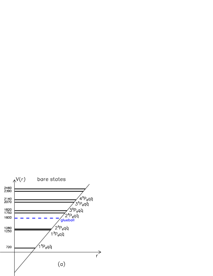
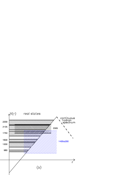
FIG. 11.: The $f_{0}$-levels in the potential well depending on the onset of the decay channels: bare states (a)
and real resonances (b).

FIG. 12.: Linear trajectories on the $(n,M^{2})$ plane for bare states (a) and resonances (b).

 

3. Where is the lightest pseudoscalar glueball?
In the pseudoscalar sector, in the mass region under discussion, one may expect the lightest pseudoscalar glueball, though the opinions about the mass of pseudoscalar glueball are rather different. According to lattice gluodynamic calculations, the mass of the lightest pseudoscalar glueball coincides with that of the tensor glueball, that is, it must be in the range 2100–2600 MeV [18], while, according to [19], its mass is close to that of the lightest scalar glueball: 1300–1700 MeV. The plausible existence of the light $0^{-+}$ glueball looks nice, for it might explain a considerable production of the $0^{-+}$ states in the radiative $J/\psi$ decay, in particular, $J/\psi\to\gamma\eta^{\prime}$ (according to [20], the admixture of the gluonium component in $\eta^{\prime}$ may be rather large, about 10%–20%). However, among narrow resonances one cannot see the candidates for pseudoscalar glueball: $\eta(1295)$ and $\eta(1440)$ lay on linear $q\bar{q}$ trajectories (Fig. 4c), though in [21] it was estimated that the value of $gg$ component in the $\eta(1440)$ can be not small, $20\%\pm 20\%$. Still, it is possible that pseudoscalar glueball, after the onset of decay channels, turned into the broad state in the region 1400–1500 MeV (as it occurred with scalar one) — the experimental data do not contradict this suggestion, see [22] and [23].

I am indebted to A.V. Anisovich, D.V. Bugg, L.G. Dakhno, V.A. Nikonov, A.V. Sarantsev for the interest to the problem under discussion. The paper is supported by RFFI grant N 01-02-17861.

REFERENCES

- [1] A.V. Anisovich, C.A. Baker, C.J. Batty et al., Phys. Lett. B449, 114 (1999); B452, 173 (1999); B 452, 180 (1999); B 452, 187 (1999); B 472, 168 (2000); B 476, 15 (2000); B 477, 19 (2000); B 491, 40 (2000); B 491, 47 (2000); B 496, 145 (2000); B 507, 23 (2001); B 508, 6 (2001); B 513, 281 (2001); B 517, 261 (2001); B 517, 273 (2001); Nucl. Phys. A 651, 253 (1999); A 662, 319 (2000); A 662, 344 (2000).
- [2] A.V. Anisovich, V.V. Anisovich, and A.V. Sarantsev, Phys. Rev. D 62:051502 (2000); A.V. Anisovich, V.V. Anisovich, and A.V. Sarantsev, Meson spectrum from the analysis of the Crystal Barrel data, in: PNPI XXX, Scientific Highlights, Theoretical Physics Division, p.58, Gatchina, 2001.
- [3] V.V. Anisovich, Systematics of quark-antiquark states and scalar exotic mesons, hep-ph/0208123.
- [4] Particle Data Group, Eur. Phys. J. C15, 1 (2000).
- [5] V.V.Anisovich, A.V. Sarantsev, Eur.Phys.J. A16, 229 (2003); Yad.Fiz. 66, 690 (2003) [Phys.Atom.Nucl. 66, 928 (2003)].
- [6] V.V. Anisovich, UFN 168 481 (1998) [Physics-Uspekhi, 41 419 (1998)]; V.V. Anisovich, A.A. Kondashov, Yu.D. Prokoshkin, S.A. Sadovsky, A.V. Sarantsev, Yad.Fiz. 60, 1489 (2000) [Phys.Atom.Nucl. 60, 1410 (2000)]; hep-ph/9711319 (1997).
- [7] A.V. Anisovich and A.V. Sarantsev, Phys. Lett. B413, 137 (1997).
- [8] V.V. Anisovich and A.V. Sarantsev, Phys. Lett. B 382, 429 (1996).
- [9] D. Alde et al., Zeit.Phys. C 66, 375 (1995); Yu.D. Prokoshkin et al., Physics – Doklady, 342, 473 (1995).
- [10] F. Binon et al., Nuovo Cim. A 78, 313 (1983); 80, 363 (1984).
- [11] S.J. Lindenbaum, R.S. Longacre, Phys.Lett. B 274, 492 (1992); A. Etkin et al., Phys.Rev. D 25, 1786 (1982).
- [12] G. Grayer et al., Nucl.Phys. B 75, 189 (1974); W. Ochs, PhD Thesis, Münich University (1974).
- [13] V.V. Anisovich, D.S. Armstrong, I. Augustin et al., Phys.Lett. B 323, 233 (1994).
- [14] C. Amsler, V.V. Anisovich, D.S. Armstrong et al., Phys.Lett. B 333, 277 (1994); D.V. Bugg, V.V. Anisovich, A.V. Sarantsev, B.S. Zou, Phys.Rev. D 50, 4412 (1994); C. Amsler et al., Phys.Lett. B342, 433 (1995); B355, 425 (1995).
- [15] A. Abele et al., Phys. Rev. D 57, 3860 (1998); Phys. Lett. B 391, 191 (1997); B 411, 354 (1997); B 450, 275 (1999); B 468, 178 (1999); B 469, 269 (1999); K. Wittmack, PhD Thesis, Bonn University, (2001); A.V.Sarantsev, talk at HADRON2003 Conference (2003).
- [16] J. Gunter et al., (E852 Collaboration), Phys.Rev. D 64:07003 (2001).
- [17] K. Peters and E. Klempt, Phys. Lett. B 352, 467 (1995).
- [18] G.S. Bali et al. Phys. Lett. B 309, 378 (1993).
- [19] L. Faddeev, A.J. Niemi and U. Wiedner, Glueballs, closed flux tubes and , hep-ph/0308240 (2003).
- [20] V.V. Anisovich, D.V. Bugg, D.I Melikhov, and V.A. Nikonov, Phys. Lett. B 404, 166 (1997).
- [21] A.V. Anisovich, Quark-gluon content of and , hep-ph/0104005 (2001).
- [22] V.V. Anisovich, UFN 165, 1225 (1995) [Physics Uspekhi 38, 1179 (1995)].
- [23] Z. Bai et al., Phys. Rev. Lett. 65, 2507 (1990). Phys. Rev. Lett. 65, 2507 (1990).