Cancellation of infrared divergences at NNLO

Abstract

Perturbative calculations at next-to-next-to-leading order for multi-particle final states require a method to cancel infrared singularities. I discuss how to setup the subtraction method at NNLO.

1 Introduction

The next generation of collider experiments will hunt for the Higgs and other yet-to-be-discovered particles with increased luminosity and experimental precision. The increased experimental precision has to be matched by an improvement in the accuracy of theoretical predictions. Theoretical predictions are calculated as a power expansion in the coupling. Higher precision is reached by including the next higher term in the perturbative expansion. The experimental needs are numerical programs which yield predictions for a wide range of observables. Urgently needed are therefore fully differential next-to-next-to-leading order (NNLO) programs. Compared to certain specific NNLO prediction for inclusive observables, these programs are flexible and allow to take into account complicated detector geometries and jet definitions. The only requirement on the observable is infrared-safety. At NNLO this implies that whenever a $n+1$ parton configuration $p_{1}$,…,$p_{n+1}$ becomes kinematically degenerate with a $n$ parton configuration $p_{1}^{\prime}$,…,$p_{n}^{\prime}$ we must have

$${\cal O}_{n+1}(p_{1},...,p_{n+1}) \rightarrow {\cal O}_{n}(p_{1}^{\prime},...,p_{n}^{\prime}).$$

In addition, we must have in the double unresolved case (e.g. when a $n+2$ parton configuration $p_{1}$,…,$p_{n+2}$ becomes kinematically degenerate with a $n$ parton configuration $p_{1}^{\prime}$,…,$p_{n}^{\prime}$)

$${\cal O}_{n+2}(p_{1},...,p_{n+2}) \rightarrow {\cal O}_{n}(p_{1}^{\prime},...,p_{n}^{\prime}).$$

To construct such NNLO programs the following ingredients are needed:

•

- The scattering amplitudes. This implies in particular for a NNLO program the calculation of the relevant two-loop amplitudes. There has been substantial progress in this field in the past years. The state-of-the-art is that all two-loop-amplitudes, which are needed most urgently, are now known Bern:2000ie ; Bern:2000dn ; Anastasiou:2000kg ; Anastasiou:2000ue ; Anastasiou:2000mv ; Anastasiou:2001sv ; Glover:2001af ; Bern:2001dg ; Bern:2001df ; Bern:2002tk ; Garland:2001tf ; Garland:2002ak ; Moch:2002hm .

•

- A NNLO program requires a method to cancel infrared divergences. Loop amplitudes, calculated in dimensional regularization, have explicit poles in the dimensional regularization parameter $\varepsilon=2-D/2$, arising from infrared singularities. These poles cancel with similar poles arising from amplitudes with additional partons, when integrated over phase space regions where two (or more) partons become “close” to each other. However, the cancellation occurs only after the integration over the unresolved phase space has been performed and prevents thus a naive Monte Carlo approach for a fully exclusive calculation. It is therefore necessary to cancel first analytically all infrared divergences and to use Monte Carlo methods only after this step has been performed.

•

- The final numerical computer program, which evaluates the remaining phase space integrals, requires stable and efficient Monte Carlo methods for this integration.

In this talk I focus on the cancellation of infrared divergences Weinzierl:2003fx ; Weinzierl:2003ra . In the next section I review general methods at NLO. In sect. 3 I discuss the subtraction method at NNLO. Sect. 4 is devoted to one-loop amplitudes with one unresolved parton.

2 A review of the subtraction method at NLO

Infrared divergences occur already at next-to-leading order. As a simple example two diagrams contributing to the NLO corrections to $e^{+}e^{-}\rightarrow\mbox{2 jets}$ are shown in fig. 1. The diagrams are divided into virtual and real corrections. The virtual corrections contain the loop integrals and can have, in addition to ultraviolet divergences, infrared divergences. For one-loop amplitudes the IR divergences manifest themselves as explicit poles in $\varepsilon$ up to $1/\varepsilon^{2}$.

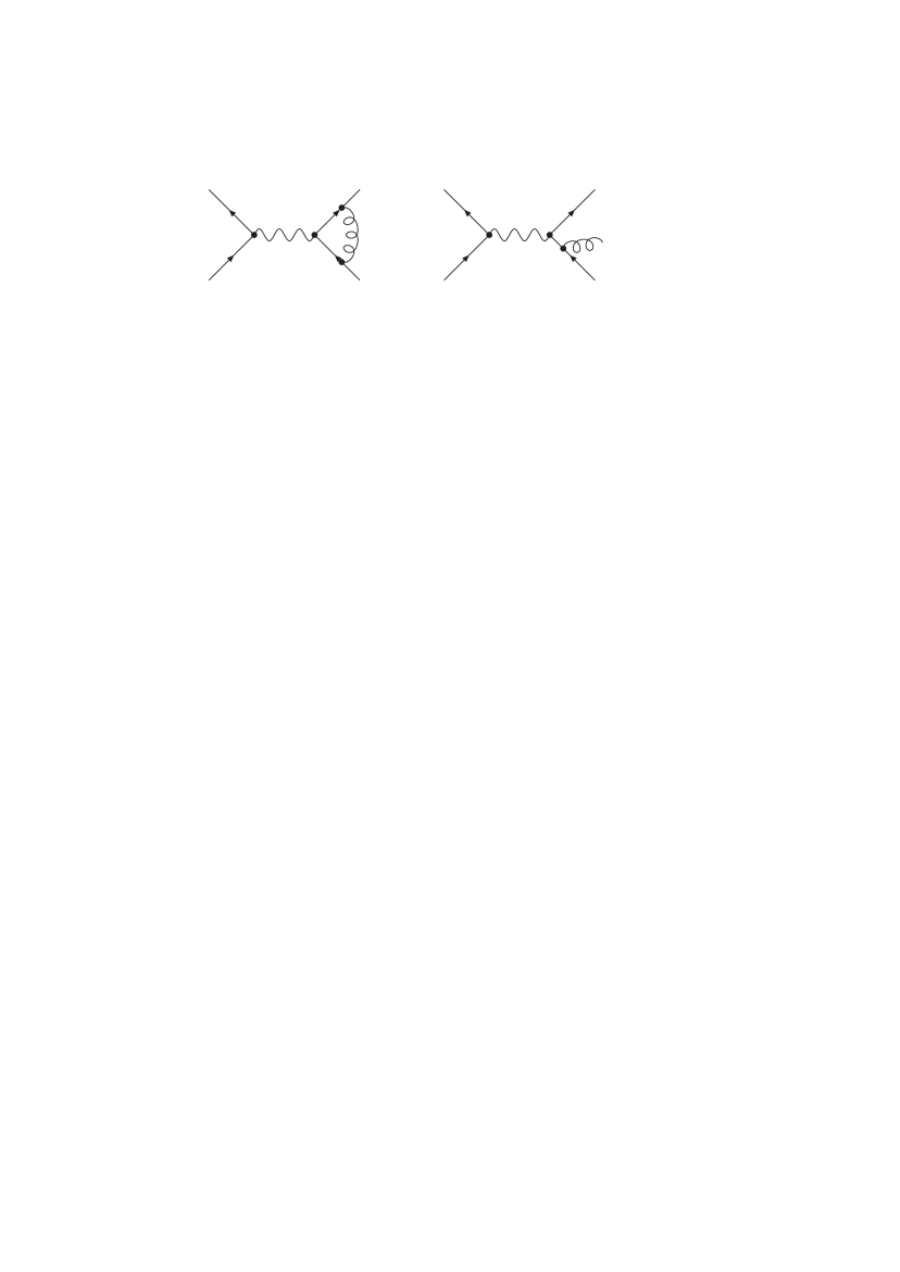
Figure 1: Cancellation of divergences between virtual and real corrections at NLO.

For each IR divergence in the virtual corrections there is a corresponding divergence with the opposite sign in the real emission amplitude, obtained from the integration over the phase space region where some particles become soft or collinear (e.g. unresolved). In general, the Kinoshita-Lee-Nauenberg theorem guarantees that any infrared-safe observable, when summed over all states degenerate according to some resolution criteria, will be finite. However, the two contributions (virtual and real) live on different phase spaces and prevent a naive Monte Carlo approach. At NLO, general methods to circumvent this problem are known. This is possible due to the universality of the singular behaviour of the amplitudes in soft and collinear limits. Examples are the phase-space slicing method Giele:1992vf ; Giele:1993dj ; Keller:1998tf and the subtraction method Frixione:1996ms ; Catani:1997vz ; Dittmaier:1999mb ; Phaf:2001gc ; Catani:2002hc . I briefly review the subtraction method here. The NLO cross section is given as the sum of the virtual and real corrections:

$$\sigma^{NLO} = \int\limits_{n+1}d\sigma^{R}+\int\limits_{n}d\sigma^{V}.$$

If one can find an approximation term $d\sigma^{A}$ such that

• $d\sigma^{A}$ has the same point-wise singular behaviour in $D$ dimensions as $d\sigma^{R}$ itself,

• $d\sigma^{A}$ can be integrated analytically in $D$ dimensions over the one-parton subspace leading to soft and collinear divergences,

then one can add and subtract this term as follows:

$$\sigma^{NLO} = \int\limits_{n+1}\left(d\sigma^{R}-d\sigma^{A}\right)+\int\limits_{n}\left(d\sigma^{V}+\int\limits_{1}d\sigma^{A}\right).$$

Since by definition $d\sigma^{A}$ has the same singular behaviour as $d\sigma^{R}$, $d\sigma^{A}$ acts as a local counter-term and the combination $(d\sigma^{R}-d\sigma^{A})$ is integrable and can be evaluated numerically. Secondly, the analytic integration of $d\sigma^{A}$ over the one-parton subspace will yield the explicit poles in $\varepsilon$ needed to cancel the corresponding poles in $d\sigma^{V}$.

3 The subtraction method at NNLO

The following terms contribute at NNLO:

$$d\sigma_{n+2}^{(0)} = \left(\left.{\cal A}_{n+2}^{(0)}\right.^{\ast}{\cal A}_{n+2}^{(0)}\right)d\phi_{n+2},$$

$$d\sigma_{n+1}^{(1)} = \left(\left.{\cal A}_{n+1}^{(0)}\right.^{\ast}{\cal A}_{n+1}^{(1)}+\left.{\cal A}_{n+1}^{(1)}\right.^{\ast}{\cal A}_{n+1}^{(0)}\right)d\phi_{n+1},$$

$$d\sigma_{n}^{(2)} = \left(\left.{\cal A}_{n}^{(0)}\right.^{\ast}{\cal A}_{n}^{(2)}+\left.{\cal A}_{n}^{(2)}\right.^{\ast}{\cal A}_{n}^{(0)}+\left.{\cal A}_{n}^{(1)}\right.^{\ast}{\cal A}_{n}^{(1)}\right)d\phi_{n},$$

where ${\cal A}_{n}^{(l)}$ denotes an amplitude with $n$ external partons and $l$ loops. $d\phi_{n}$ is the phase space measure for $n$ partons. Taken separately, each of these contributions is divergent. Only the sum of all contributions is finite. To render the individual contributions finite, one adds and subtracts suitable pieces:

$$\langle{\cal O}\rangle_{n}^{NNLO}=$$

$$\int\left({\cal O}_{n+2}\;d\sigma_{n+2}^{(0)}-{\cal O}_{n+1}\circ d\alpha^{(0,1)}_{n+1}-{\cal O}_{n}\circ d\alpha^{(0,2)}_{n}\right)$$

$$+\int\left({\cal O}_{n+1}\;d\sigma_{n+1}^{(1)}+{\cal O}_{n+1}\circ d\alpha^{(0,1)}_{n+1}-{\cal O}_{n}\circ d\alpha^{(1,1)}_{n}\right)$$

$$+\int\left({\cal O}_{n}\;d\sigma_{n}^{(2)}+{\cal O}_{n}\circ d\alpha^{(0,2)}_{n}+{\cal O}_{n}\circ d\alpha^{(1,1)}_{n}\right).$$

Here $d\alpha_{n+1}^{(0,1)}$ is a subtraction term for single unresolved configurations of Born amplitudes. This term is already known from NLO calculations. The term $d\alpha_{n}^{(0,2)}$ is a subtraction term for double unresolved configurations. Finally, $d\alpha_{n}^{(1,1)}$ is a subtraction term for single unresolved configurations involving one-loop amplitudes.

To construct these terms the universal factorization properties of QCD amplitudes in unresolved limits are essential. QCD amplitudes factorize if they are decomposed into primitive amplitudes. Primitive amplitudes are defined by a fixed cyclic ordering of the QCD partons, a definite routing of the external fermion lines through the diagram and the particle content circulating in the loop.

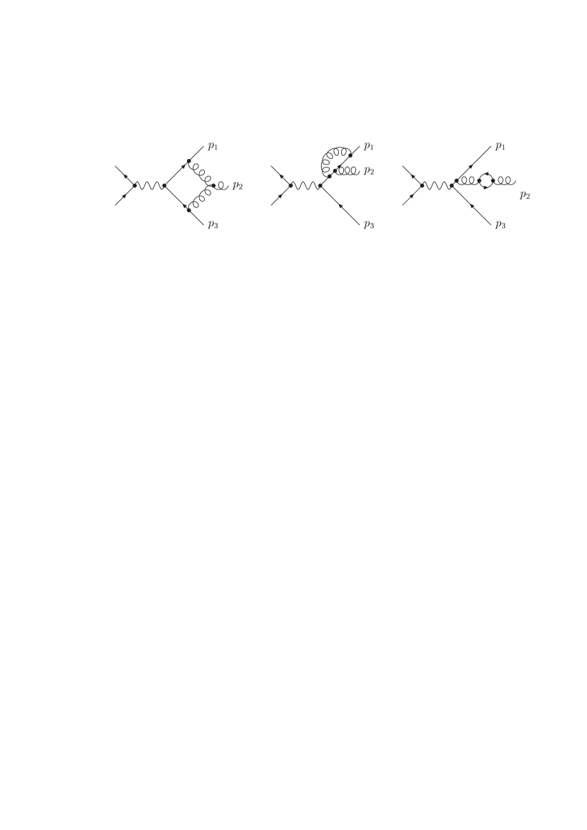
Figure 2: Diagrams contributing to different primitive amplitudes.

Fig. 2 shows three one-loop diagrams for $e^{+}e^{-}\rightarrow\mbox{3 jets}$ contributing to different primitive amplitudes. One-loop amplitudes factorize in single unresolved limits as Bern:1994zx ; Bern:1998sc ; Kosower:1999xi ; Kosower:1999rx ; Bern:1999ry ; Catani:2000pi ; Kosower:2003cz

$$A^{(1)}_{n} = \mbox{Sing}^{(0,1)}\cdot A^{(1)}_{n-1}+\mbox{Sing}^{(1,1)}\cdot A^{(0)}_{n-1}.$$ (1)

Tree amplitudes factorize in the double unresolved limits as Berends:1989zn ; Gehrmann-DeRidder:1998gf ; Campbell:1998hg ; Catani:1998nv ; Catani:1999ss ; DelDuca:1999ha ; Kosower:2002su

$$A^{(0)}_{n} = \mbox{Sing}^{(0,2)}\cdot A^{(0)}_{n-2}.$$

To discuss the term $d\alpha_{n}^{(0,2)}$ let us consider as an example the Born leading-colour contributions to $e^{+}e^{-}\rightarrow qgg\bar{q}$, which contribute to the NNLO corrections to $e^{+}e^{-}\rightarrow\mbox{2 jets}$. The subtraction term has to match all double and single unresolved configurations. The double unresolved configurations are:
- Two pairs of separately collinear particles,
- Three particles collinear,
- Two particles collinear and a third soft particle,
- Two soft particles,
- Coplanar degeneracy.
The single unresolved configurations are:
- Two collinear particles,
- One soft particle.
It is convenient to construct $d\alpha_{n}^{(0,2)}$ as a sum over several pieces,

$$d\alpha^{(0,2)}_{n} = \sum\limits_{\mbox{\tiny topologies $T$}}{\cal D}_{n}^{(0,2)}(T).$$

Each piece is labelled by a splitting topology.

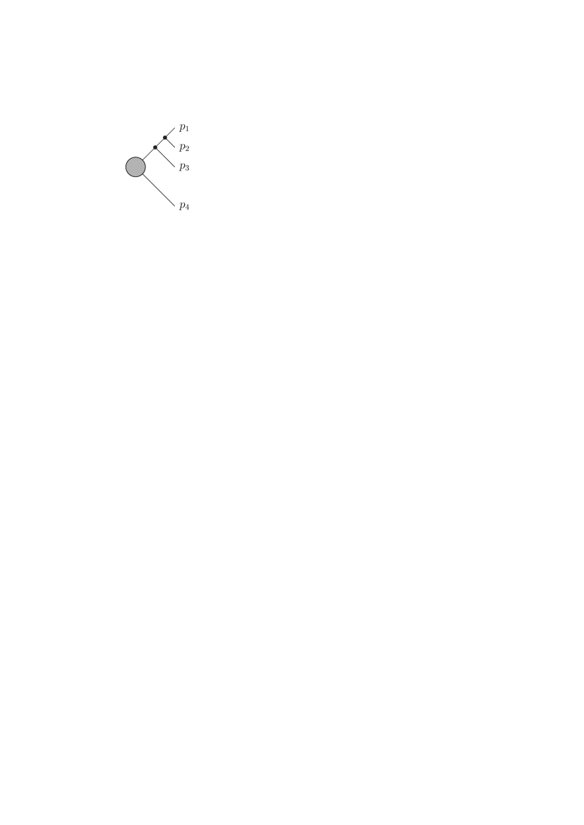
Figure 3: Splitting topology.

An example is shown in fig. 3. The term ${\cal D}_{n}^{(0,2)}(T)$ corresponding to the topology shown in fig. 3 approximates singularities in $1/s_{12}$, $1/(s_{12}s_{123})$ and part of the singularities in $1/s_{123}^{2}$. Care has to be taken to disentangle correctly overlapping singularities like $1/(s_{12}s_{23})$. Details can be found in Weinzierl:2003fx .

4 One-loop amplitudes with one unresolved parton

Apart from $d\alpha_{n}^{(0,2)}$ also the term $d\alpha_{n}^{(1,1)}$, which approximates one-loop amplitudes with one unresolved parton, is needed at NNLO. If we recall the factorization formula (1), this requires as a new feature the approximation of the one-loop singular function $\mbox{Sing}^{(1,1)}$. The corresponding subtraction term is proportional to the one-loop $1\rightarrow 2$ splitting function ${\cal P}^{(1,1)}_{(1,0)\;a\rightarrow bc}$. An example is the leading-colour part for the splitting $q\rightarrow qg$:

$${\cal P}^{(1,1)}_{(1,0)\;q\rightarrow qg,lc,corr}=-\frac{11}{6\varepsilon}{\cal P}^{(0,1)}_{q\rightarrow qg},+S_{\varepsilon}^{-1}c_{\Gamma}\left(\frac{-s_{ijk}}{\mu^{2}}\right)^{-\varepsilon}y^{-\varepsilon}$$

$$\left\{g_{1,corr}(y,z)\;{\cal P}^{(0,1)}_{q\rightarrow qg}+f_{2}\frac{2}{s_{ijk}}\frac{1}{y}p\!\!\!/_{e}\left[1-\rho\varepsilon(1-y)(1-z)\right]\right\}.$$

This term depends on the correlations among the remaining hard partons. If only two hard partons are correlated, $g_{1}$ is given by

$$g_{1,intr}(y,z)=-\frac{1}{\varepsilon^{2}}\left[\Gamma(1+\varepsilon)\Gamma(1-\varepsilon)\left(\frac{z}{1-z}\right)^{\varepsilon}+1\right.$$

$$\left.-(1-y)^{\varepsilon}z^{\varepsilon}\;{}_{2}F_{1}\left(\varepsilon,\varepsilon,1+\varepsilon;(1-y)(1-z)\right)\right].\hskip 28.45274pt$$

For the integration of the subtraction terms over the unresolved phase space all occuring integrals are reduced to standard integrals of the form

$$\int\limits_{0}^{1}dy\;y^{a}(1-y)^{1+c+d}\int\limits_{0}^{1}dz\;z^{c}(1-z)^{d}\left[1-z(1-y)\right]^{e}$$

$${}_{2}F_{1}\left(\varepsilon,\varepsilon;1+\varepsilon;(1-y)z\right)=$$

$$\frac{\Gamma(1+a)\Gamma(1+d)\Gamma(2+a+d+e)\Gamma(1+\varepsilon)}{\Gamma(2+a+d)\Gamma(\varepsilon)\Gamma(\varepsilon)}$$

$$\sum\limits_{j=0}^{\infty}\frac{\Gamma(j+\varepsilon)\Gamma(j+\varepsilon)\Gamma(j+1+c)}{\Gamma(j+1)\Gamma(j+1+\varepsilon)\Gamma(j+3+a+c+d+e)}.$$

The result is proportional to a hyper-geometric functions ${}_{4}F_{3}$ with unit argument and can be expanded into a Laurent series in $\varepsilon$ with the techniques of Moch:2001zr ; Weinzierl:2002hv . For the example discussed above one finds after integration Weinzierl:2003ra :

$${\cal V}^{(1,1)}_{(1,0)\;q\rightarrow qg,lc,intr}=-\frac{1}{4\varepsilon^{4}}-\frac{31}{12\varepsilon^{3}}+\left(-\frac{51}{8}-\frac{1}{4}\rho+\frac{5}{12}\pi^{2}\right.$$

$$\left.-\frac{11}{6}L\right)\frac{1}{\varepsilon^{2}}+\left(-\frac{151}{6}-\frac{55}{24}\rho+\frac{145}{72}\pi^{2}+\frac{15}{2}\zeta_{3}-\frac{11}{4}L\right.$$

$$\left.-\frac{11}{12}L^{2}\right)\frac{1}{\varepsilon}-\frac{1663}{16}-\frac{233}{24}\rho+\frac{107}{16}\pi^{2}+\frac{5}{12}\rho\pi^{2}+\frac{356}{9}\zeta_{3}$$

$$-\frac{1}{72}\pi^{4}-\frac{187}{24}L-\frac{11}{12}\rho L+\frac{55}{72}\pi^{2}L-\frac{11}{8}L^{2}-\frac{11}{36}L^{3}$$

$$+i\pi\left[-\frac{1}{4\varepsilon^{3}}-\frac{3}{4\varepsilon^{2}}+\left(-\frac{29}{8}-\frac{1}{4}\rho+\frac{\pi^{2}}{3}\right)\frac{1}{\varepsilon}-\frac{139}{8}-\frac{11}{8}\rho\right.$$

$$\left.+\pi^{2}+\frac{15}{2}\zeta_{3}\right]+{\cal O}(\varepsilon),$$

where $L=\ln(s_{ijk}/\mu^{2})$. The parameter $\rho$ specifies the variant of dimensional regularization: $\rho=1$ in the conventional or ’t Hooft-Veltman scheme and $\rho=0$ in a four-dimensional scheme.

5 Outlook

In this talk I reported on the subtraction method to cancel infrared divergences at NNLO. The set-up involves two new types of subtraction terms, $d\alpha^{(0,2)}_{n}$ and $d\alpha^{(1,1)}_{n}$. The former approximates double unresolved configurations of tree amplitudes with $n+2$ partons, whereas the latter approximates one-loop amplitudes in single unresolved limits. Decomposing the QCD amplitudes into partial and primitive amplitudes, the appropriate subtraction terms have been constructed. Furthermore, the analytic integration over the unresolved phase space has been performed for all terms contributing to $d\alpha^{(1,1)}_{n}$. Once the corresponding analytic integration has been done for $d\alpha^{(0,2)}_{n}$ the subtraction method at NNLO is complete and can used for fully differential programs at NNLO.

References

- (1) Z. Bern, L. Dixon, and A. Ghinculov, Phys. Rev. D63, 053007 (2001), hep-ph/0010075.
- (2) Z. Bern, L. Dixon, and D. A. Kosower, JHEP 01, 027 (2000), hep-ph/0001001.
- (3) C. Anastasiou, E. W. N. Glover, C. Oleari, and M. E. Tejeda-Yeomans, Nucl. Phys. B601, 318 (2001), hep-ph/0010212.
- (4) C. Anastasiou, E. W. N. Glover, C. Oleari, and M. E. Tejeda-Yeomans, Nucl. Phys. B601, 341 (2001), hep-ph/0011094.
- (5) C. Anastasiou, E. W. N. Glover, C. Oleari, and M. E. Tejeda-Yeomans, Phys. Lett. B506, 59 (2001), hep-ph/0012007.
- (6) C. Anastasiou, E. W. N. Glover, C. Oleari, and M. E. Tejeda-Yeomans, Nucl. Phys. B605, 486 (2001), hep-ph/0101304.
- (7) E. W. N. Glover, C. Oleari, and M. E. Tejeda-Yeomans, Nucl. Phys. B605, 467 (2001), hep-ph/0102201.
- (8) Z. Bern, A. De Freitas, L. J. Dixon, A. Ghinculov, and H. L. Wong, JHEP 11, 031 (2001), hep-ph/0109079.
- (9) Z. Bern, A. De Freitas, and L. J. Dixon, JHEP 09, 037 (2001), hep-ph/0109078.
- (10) Z. Bern, A. De Freitas, and L. Dixon, JHEP 03, 018 (2002), hep-ph/0201161.
- (11) L. W. Garland, T. Gehrmann, E. W. N. Glover, A. Koukoutsakis, and E. Remiddi, Nucl. Phys. B627, 107 (2002), hep-ph/0112081.
- (12) L. W. Garland, T. Gehrmann, E. W. N. Glover, A. Koukoutsakis, and E. Remiddi, Nucl. Phys. B642, 227 (2002), hep-ph/0206067.
- (13) S. Moch, P. Uwer, and S. Weinzierl, Phys. Rev. D66, 114001 (2002), hep-ph/0207043.
- (14) S. Weinzierl, JHEP 03, 062 (2003), hep-ph/0302180.
- (15) S. Weinzierl, JHEP 07, 052 (2003), hep-ph/0306248.
- (16) W. T. Giele and E. W. N. Glover, Phys. Rev. D46, 1980 (1992).
- (17) W. T. Giele, E. W. N. Glover, and D. A. Kosower, Nucl. Phys. B403, 633 (1993), hep-ph/9302225.
- (18) S. Keller and E. Laenen, Phys. Rev. D59, 114004 (1999), hep-ph/9812415.
- (19) S. Frixione, Z. Kunszt, and A. Signer, Nucl. Phys. B467, 399 (1996), hep-ph/9512328.
- (20) S. Catani and M. H. Seymour, Nucl. Phys. B485, 291 (1997), hep-ph/9605323; Erratum Nucl. Phys. B510, 503 (1997).
- (21) S. Dittmaier, Nucl. Phys. B565, 69 (2000), hep-ph/9904440.
- (22) L. Phaf and S. Weinzierl, JHEP 04, 006 (2001), hep-ph/0102207.
- (23) S. Catani, S. Dittmaier, M. H. Seymour, and Z. Trocsanyi, Nucl. Phys. B627, 189 (2002), hep-ph/0201036.
- (24) Z. Bern, L. Dixon, D. C. Dunbar, and D. A. Kosower, Nucl. Phys. B425, 217 (1994), hep-ph/9403226.
- (25) Z. Bern, V. Del Duca, and C. R. Schmidt, Phys. Lett. B445, 168 (1998), hep-ph/9810409.
- (26) D. A. Kosower, Nucl. Phys. B552, 319 (1999), hep-ph/9901201.
- (27) D. A. Kosower and P. Uwer, Nucl. Phys. B563, 477 (1999), hep-ph/9903515.
- (28) Z. Bern, V. Del Duca, W. B. Kilgore, and C. R. Schmidt, Phys. Rev. D60, 116001 (1999), hep-ph/9903516.
- (29) S. Catani and M. Grazzini, Nucl. Phys. B591, 435 (2000), hep-ph/0007142.
- (30) D. A. Kosower, Phys. Rev. Lett. 91, 061602 (2003), hep-ph/0301069.
- (31) F. A. Berends and W. T. Giele, Nucl. Phys. B313, 595 (1989).
- (32) A. Gehrmann-De Ridder and E. W. N. Glover, Nucl. Phys. B517, 269 (1998), hep-ph/9707224.
- (33) J. M. Campbell and E. W. N. Glover, Nucl. Phys. B527, 264 (1998), hep-ph/9710255.
- (34) S. Catani and M. Grazzini, Phys. Lett. B446, 143 (1999), hep-ph/9810389.
- (35) S. Catani and M. Grazzini, Nucl. Phys. B570, 287 (2000), hep-ph/9908523.
- (36) V. Del Duca, A. Frizzo, and F. Maltoni, Nucl. Phys. B568, 211 (2000), hep-ph/9909464.
- (37) D. A. Kosower, Phys. Rev. D67, 116003 (2003), hep-ph/0212097.
- (38) S. Moch, P. Uwer, and S. Weinzierl, J. Math. Phys. 43, 3363 (2002), hep-ph/0110083.
- (39) S. Weinzierl, Comput. Phys. Commun. 145, 357 (2002), math-ph/0201011.