Numerical simulation of vacuum particle production: applications to cosmology, dynamical Casimir effect and time-dependent non-homogeneous dielectrics

Abstract

We develop a general numerical method aimed at studying particle production from vacuum states in a variety of settings. As a first example we look at particle production in a simple cosmological model. We apply the same approach to the dynamical Casimir effect, with special focus on the case of an oscillating mirror. We confirm previous estimates and obtain long-time production rates and particle spectra for both resonant and off-resonant frequencies. Finally, we simulate a system with space and time-dependent optical properties, analogous to a one-dimensional expanding dielectric bubble. We obtain simple expressions for the dependence of the final particle number on the expansion velocity and final dielectric constant.

]

I Introduction

One of the most intriguing and fascinating features of quantum field theory resides in the non-trivial nature of its vacuum states. Quantum fluctuations present in the vacuum are responsible for non-classical effects that can be experimentally detected. The most well known of such phenomena is perhaps the Casimir effect [1]. In this setting, the vacuum energy between two static metallic plates is shifted due to quantum fluctuations, resulting in an attractive force between the plates. In general non-static situations, changes in a system’s parameters may lead to a redefinition of the natural vacuum state. As a result, a system initially in the vacuum may at later stages display a non-zero particle content. The possibility of this type of particle production mechanism has been identified and studied in a large variety of systems. In a cosmological context, particle creation may occur in back-hole radiation - the Hawking effect [2], and as a consequence of an expanding gravitational background [3]. In the laboratory it is possible that dynamical generalisations of the Casimir effect may lead to observable effects [4]. Alternatively, there have been efforts to reproduce the Hawking effect using specific matter systems [5, 6]. This is the case of slow-light experiments [7], black-hole sonic analogues in Bose-Einstein condensates [8] and dielectric media [9].

The calculations involved in determining the physical outcome of particle creation processes, though trivial to state, are often hard or impossible to complete. Usually one is required to find the solution of a set of space and/or time-dependent field equations, with initial conditions covering a complete basis of functions. Even when relying on simplifying approximations, the set of problems for which solutions can be found is considerably limited. On the other hand, linear partial differential equations are relatively easy to solve numerically, and the above task is within present computational capabilities. In this paper we explore this possibility and introduce a fully numerical scheme for studying particle production in general settings. We will use examples with known solutions to help developing and testing the required numerical techniques. These will then be applied to new cases, extending original predictions and leading to new results.

In Section II, we rely on a simple cosmological example to introduce notation and discuss concepts relevant for the rest of the paper. We use this system to describe the general numerical approach and we test it, by comparing the results with known analytical predictions. In Section III, we apply these techniques to the case of particle creation by a reflecting moving boundary in a one-dimensional cavity. For an oscillating motion we obtain particle production rates and spectra, for both resonant and non-resonant frequencies, in the short and long-time regimes. In Section IV, we study a system with time dependent optical properties, mimicking a bubble of dielectric material expanding into the vacuum. From the numerical data we determine the dependence of the final particle number on the expansion velocity and strength of the dielectric. Finally, in Section V we discuss our results and suggest further applications. Appendix A contains a description of the numerical algorithm used in Section III to solve the field equations for moving boundary conditions.

II A First Example: Particle Creation in an Expanding Background

In this section we will look at a simple example of particle creation in a cosmological system. In particular, we will study the evolution of a free complex field $\phi$ in an expanding flat universe. Here and throughout the paper we will follow the conventions and notation of reference[3].

For a general gravitational background, the equation of motion for a scalar field is given by

$$(-g)^{-1/2}\partial_{\mu}[(-g)^{1/2}g^{\mu\nu}\partial_{\nu}\phi]+m^{2}\phi=0,$$ (1)

where $g_{\mu\nu}$ is the space-time metric and $g=|\det g_{\mu\nu}|$.

The invariant scalar product of any two solutions of Eq. (1) is defined as

$$(\phi_{1},\phi_{2})=-i\int_{\Sigma}\left[\phi_{1}\,\partial_{\mu}\phi^{*}_{2}-\partial_{\mu}\phi_{1}\,\phi^{*}_{2}\right]\sqrt{-g_{\Sigma}}\,d\Sigma^{\mu},$$ (2)

where the integral is taken over any space-like surface of the space-time ($d\Sigma^{\mu}$ is the time-like unit-vector orthogonal to the surface). Using Eq. (2) we can construct orthonormal basis of solutions of the equations of motion, obeying:

$$(u_{i},u_{j})=\delta_{ij},\,\,\,\,\,\,(u_{i}^{*},u_{j}^{*})=-\delta_{ij},\,\,\,\,\,\,(u_{i},u_{j}^{*})=0$$ (3)

Expanding the field operator in terms of a given basis we obtain the familiar creation and annihilation operators $a_{i}^{\dagger}$, $a_{i}$:

$$\phi(x)=\sum_{i}\,[a_{i}u_{i}(x)+a_{i}^{\dagger}u_{i}^{*}(x)]$$ (4)

Particle states are defined in respect to $a_{i}^{\dagger}$, $a_{i}$. In general we will be looking at systems which are static and flat for both early and late times - the so called in-out type problems. For these cases we can single-out in a natural way, two different basis of solutions, $\{u^{\rm in}_{i}\}$ and $\{u^{\rm out}_{j}\}$ which tend respectively as $t\rightarrow t_{\rm in}$ and $t\rightarrow t_{\rm out}$, to the usual flat-space positive frequency modes. The field can be quantised in terms of any of these two basis, leading to different definitions of creation and annihilation operators and hence to different definitions of particle states. In most cases of interest, the particle content of a given state will change depending on the set of modes we chose as basis. In particular, we will consider the case where the system is in the vacuum state corresponding to the in modes. In respect to the out particle states - the natural choice for late times - this state may have a non-zero particle content. The particle spectrum is given by [3]

$$N_{i}=\sum_{j}|\beta_{ij}|^{2}$$ (5)

where $N_{i}$ is the number of particles in the mode $i$. The $\beta_{ij}$’s are a subset of the so-called Bogolugov coefficients which relate the two basis and can be evaluated using [3]:

$$\alpha_{ij}=(u_{i}^{\rm out},u_{j}^{\rm in}),\,\,\,\,\,\,\beta_{ij}=-(u_{i}^{\rm out},[u_{j}^{\rm in}]^{*})$$ (6)

In this paper, we will look into how to tackle the calculation of the particle spectrum for general in-out problems, using a fully numerical approach. We will start by evaluating numerically the in modes $\{u^{\rm in}_{i}\}$. This is done by solving the equation of motion Eq. (1), taking as initial condition the asymptotic, flat-space mode solutions corresponding to the Minkowsky vacuum. These are propagated up to $t_{\rm out}$, when the new stationary flat configuration is reached. The resulting in modes can then be contracted with the out modes, by evaluating numerically the integral Eq. (2) at $t=t_{\rm out}$. In this way we obtain the Bogolugov coefficients Eq. (6). Other physical quantities, such as the particle spectrum can be evaluated in terms of these.

To illustrate the method, we look at a simple example of a $1+1$ space-time with a time dependent scale factor. In conformal coordinates, the metric is given by

$${\rm d}s^{2}=a^{2}(\eta)({\rm d}\eta^{2}-{\rm d}x^{2}),$$ (7)

and the field equations of motion are

$$\frac{\partial^{2}\phi}{\partial\eta^{2}}=\frac{\partial^{2}\phi}{\partial x^{2}}-m^{2}a^{2}(\eta)\phi$$ (8)

For this system, the time independent inner product of two solutions is given by

$$(\phi_{1},\phi_{2})=-i\int_{-\infty}^{+\infty}\left[\phi_{1}\,\partial_{\eta}\phi^{*}_{2}-\partial_{\eta}\phi_{1}\,\phi^{*}_{2}\right]\,dx$$ (9)

We take $a(\eta)\rightarrow a_{\rm in}$ as $\eta\rightarrow-\infty$, and $a(\eta)\rightarrow a_{\rm out}$ as $\eta\rightarrow+\infty$. In these limits, the corresponding mode basis have the usual flat space-time form:

$$u^{\rm in}_{k}\rightarrow\frac{1}{2\sqrt{\pi\omega_{\rm in}}}e^{ikx-i\omega_{\rm in}\eta},\,\,\,\,\,\omega_{\rm in}=\sqrt{k^{2}+m^{2}a_{\rm in}^{2}}$$ (10)

$$u^{\rm out}_{k}\rightarrow\frac{1}{2\sqrt{\pi\omega_{\rm out}}}e^{ikx-i\omega_{\rm out}\eta},\,\,\,\,\,\omega_{\rm out}=\sqrt{k^{2}+m^{2}a_{\rm out}^{2}}$$ (11)

For the scale-factor $a(\eta)$ we choose a particular form for which there is a known analytical solution [3]:

$$a^{2}(\eta)=\frac{1}{2}(a_{\rm out}^{2}+a_{\rm in}^{2})+\frac{1}{2}(a_{\rm out}^{2}-a_{\rm in}^{2})\,{\rm tanh}(\rho\eta)$$ (12)

Taking Eq. (10) as initial condition, we evolve the equation of motion Eq. (8) up to a time when $a\sim a_{\rm out}$. The numerical solutions are then contracted with the out modes Eq. (11), using Eq. (9) to obtain the Bogolugov coefficients. For our choice of scale-factor these can be evaluated analytically. The derivation can be found in [3], the result being given by

$$|\alpha_{kk^{\prime}}|^{2}=\delta_{kk^{\prime}}\frac{\sinh^{2}[\pi(\omega_{\rm out}+\omega_{\rm in})/(2\rho)]}{\sinh(\pi\omega_{\rm in}/\rho)\sinh(\pi\omega_{\rm out}/\rho)}$$ (13)

$$|\beta_{kk^{\prime}}|^{2}=\delta_{kk^{\prime}}\frac{\sinh^{2}[\pi(\omega_{\rm out}-\omega_{\rm in})/(2\rho)]}{\sinh(\pi\omega_{\rm in}/\rho)\sinh(\pi\omega_{\rm out}/\rho)}$$ (14)

In Fig. 1 we compare the numerical Bogolugov coefficients with the expected analytical values, for a particular choice of parameters $m=1$, $\rho=10.$, $a_{\rm in}=1.$ and $a_{\rm out}=10.$ We evolved $40$ modes for a period of time $t_{\rm out}-t_{\rm in}=0.6$, enough for the scale factor to change from its initial to final value with good accuracy. The equation of motion Eq. (8) was discretized using a standard Leap-Frog algorithm, in a box of physical size $L=100$ with periodic boundary conditions. The lattice spacing and time-step were set to $dx=0.25$ and $dt=0.0001$. The numerical data matches very well the analytical prediction, confirming the accuracy of the numerical approach for the chosen set of parameters.

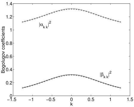
FIG. 1.: Analytical (line) and numerical results (crosses) for Bogolugov coefficients, for a model with $m=1$, $\rho=10.$, $a_{\rm in}=1.$ and $a_{\rm out}=10$.

Note that only diagonal elements of the Bogolugov matrix are non-zero, a consequence of the invariance of the system under spatial translations. This implies that the particle spectrum coincides with the diagonal of the Bogolugov matrix, i.e. $N_{k}=|\beta_{kk}|^{2}$. Since Eq. (8) is separable in space and time, we would have the choice of evolving independently each mode’s amplitude in Fourier space. Numerically this approach would have been considerably simpler. Our method is crucial though, in situations where this option is not available. In the next sections we will apply it to a few of such cases, systems that have both explicit space and time-dependency.

III Particle Production by a Moving Mirror in a Cavity

In this section we will look at particle production by a moving mirror in a closed cavity. This system has attracted the attention of several authors, displaying many complex and non-trivial features despite its apparent simplicity. More importantly, it is the most natural setting for an experimental observation of particle creation from a vacuum state (see [4] and references therein).

We will consider a scalar field confined to a one-dimensional box with one of the boundaries fixed at $x=0$ and the other moving according to a given trajectory $X(t)$ (with $|\dot{X}(t)|<1$). For the sake of simplicity, and in order to take advantage of conformal invariance we assume the field to be massless, its equation of motion being given by

$$\frac{\partial^{2}\phi}{\partial t^{2}}=\frac{\partial^{2}\phi}{\partial x^{2}}$$ (15)

The boundary conditions for the field are obtained by constraining it to vanish on both walls at all times, i.e. $\phi(0,t)=\phi(X(t),t)=0$. By doing so we assume the walls to be perfect reflectors.

In the case of a stationary mirror, time translational invariance makes it possible to find a set of mode solutions with positive definite frequency. These are given by

$$u_{n}(x,t)=\frac{1}{\sqrt{n\pi}}e^{-i\omega_{n}t}\sin(\omega_{n}x),$$ (16)

$$\,\,\,\,\,\omega_{n}=\frac{n\pi}{L}\,\,\,\,\,\,\,\,n=1,\dots,\infty$$ (17)

where $L$ is the length of the static box. These modes and their complex conjugates form a complete set of solutions of Eq. (15), orthonormal in respect to the simplectic product

$$(\phi_{1},\phi_{2})=-i\int_{0}^{L}\left[\phi_{1}\,\partial_{t}\phi^{*}_{2}-\partial_{t}\phi_{1}\,\phi^{*}_{2}\right]\,dx$$ (18)

The stationary solution allows us to define a general class of in-out problems. We will consider mirror trajectories such that $X(t)$ is a constant $X_{0}$ for $t<0$, evolves arbitrarily for a period of time, going back to rest at $X_{f}$ for $t>t_{f}$. The time and space dependence introduced in the system by the motion of the mirror, leads to particle production without the need to consider additional external fields. This phenomenon is known as the dynamical Casimir effect.

In order to determine the final particle content of the box for a given $X(t)$, one must find a set of solutions for the equation of motion, using Eq. (27) as initial condition. This problem can be formally solved by taking advantage of the conformal invariance of Eq. (15). G. Moore showed [10] (see also [11]) that by changing coordinates, the general problem can be mapped into the stationary case. In this way a complete set of solutions can be found, with the general form $u_{n}(x,t)\propto\exp[-in\pi R(t-x)]-\exp[-in\pi R(t+x)]$. $R(u)$ is a function to be determined in terms of the particular motion of the mirror, according to [10]

$$R[t+X(t)]=R[t-X(t)]+2$$ (19)

This equation is of course non-trivial to solve in generality. One approach is to find $R(u)$ in terms of $X(t)$ via a perturbative expansion in the velocity of the mirror [10]. This technique is valid only in the adiabatic limit $\dot{X}<<1$ and gives no meaningful results in the relativistic regime. Only for a few specific cases of the mirrors’s trajectory have analytical solutions been found [12, 13, 14, 15].

Using the numerical procedure outlined in Section II the problem can be solved for any given arbitrary mirror trajectory. The known analytical solutions will be useful in providing tests for the algorithms and in gauging the numerical requirements for good accuracy. The general procedure will be as before: the in-modes Eq. (27) are evolved numerically up to the final time $t_{\rm f}$, when the result is contracted with the basis of stationary modes for the final length $X_{\rm f}$. The main difficulty lies in obtaining a numerical solution for the wave equation with moving boundaries. Since the size of the box changes with time we are forced to vary the number of points in the simulation lattice. These discontinuous jumps in the lattice size introduce errors in the numerical solution. We overcame the problem by developing an improved Leap-Frog algorithm that smoothes the values of the field derivatives on the boundary - a detailed discussion of the method can be found in Appendix A.

Finally we should stress that although the focus here will be on one dimensional massless field theories, the same methods can easily be extended to higher dimensions and massive fields [16]. In those cases very few results are known [17] since one cannot rely on conformal invariance to simplify the problem. For those systems, a numerical approach may be the only way to tackle accurately the long time regime.

A Uniformly Moving Mirror

Here we will look briefly at a simple type of trajectory for which the in-out problem can be solved analytically [10, 11, 12], namely the case when the mirror moves with constant velocity. The mirror evolves from rest at $t=0.$ moving according to $X(t)=X_{0}+vt$ up to final time $t_{f}$, when it becomes stationary again. The function $R(u)$ obeying Eq. (19) for this trajectory was fully determined by Castagnino and Ferraro [12]. These authors showed that $R$ is a piece-wise linear function with derivative discontinuities. This is a consequence of the discontinuous change in the velocity of the mirror for initial and final times. The final spectrum for created particles was estimated to be of the form $N(k)\propto v^{2}/k$, in the limit of large $k$ and velocities much lower than the speed of light.

In Fig. 2 we confirm this estimate. The results were obtained by simulating a box with initial physical length $X_{0}=50.$ expanding with constant speed $v$ for a total time $t_{f}=50.$ We evaluated the final particle spectrum for $20$ modes, for values of $v$ ranging from $0.1$ to $0.9$. As seen in the figure, the spectrum for high $k$ is well fitted by a power law of the form $N(k)=Bk^{\alpha}$, with $B$ and $\alpha$ depending on $v$. As expected, $\alpha$ is close to $-1$, varying between $-1.1$ for $v=0.1$ and $-1.3$ for $v=0.9$. $B$ also depends quadratically on the expansion velocity for small $v$. When relativistic speeds are reached (about $v\sim.7$) this simple relation stops holding, with $B$ increasing faster and leading to a stronger rate of particle production.

Note that the $1/k$ spectrum leads to a logarithmically divergent total particle number. This divergence is a consequence of the discontinuous changes in the velocity of the mirror [10]. As a rule of thumb we may expect particle production to be related to the mirror’s acceleration. As this diverges for the initial and final times, so does the total particle number. In realistic cases however, the divergence should disappear, as the acceleration remains bounded for all times.

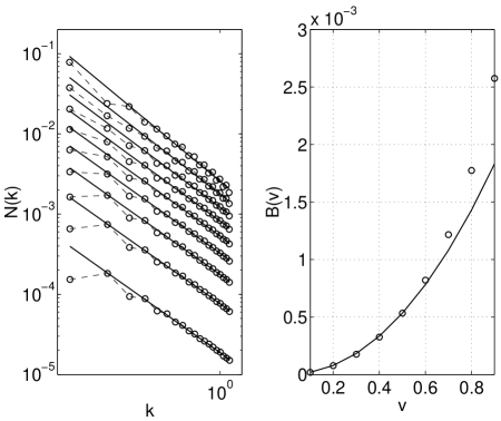
FIG. 2.: Left plot: particle spectrum for mirror velocities varying from $0.1$ to $0.9$ (bottom to top). The straight lines are fits to a power law $N=Bk^{\alpha}$, using the 15 higher momentum data points. In the right plot we have the dependence of $B$ on the velocity. For low-$v$ this is well described by $B=v^{2.1}$, the numerical power being obtained by fitting the first $6$ data points.

Finally let us note that for a box that expands continuously with constant $v$, with no initial or final stationary points, an exact solution for Eq. (19) can easily obtained [10]:

$$R(u)=\frac{1}{\arctan{v}}\log\left(u+\frac{X_{0}}{v}\right)$$ (20)

with $X_{0}$ the position of the mirror at $t=0$. The corresponding normalised mode basis is given by

$$v_{n}=\frac{1}{2\sqrt{n\pi}}\left[e^{-i\Omega_{n}\log(X_{0}/v+t-x)}-e^{-i\Omega_{n}\log(X_{0}/v+t+x)}\right],$$ (21)

$$\,\,\,\,\,\Omega_{n}=\frac{n\pi}{{\rm arctanh}(v)}\,\,\,\,\,\,\,\,n=1,\dots,\infty$$ (22)

This set of exact analytical solutions proved useful in testing the accuracy of the numerical algorithm for the moving boundary problem, as detailed in Appendix A. An interesting feature of the solution is that for $t_{r}=2X_{0}/(1-v)$ the evolved modes coincide with the original ones, re-scaled to the new box length. This feature is also present for the in-out motion studied above. It implies that at $t_{r}$ the in modes are identical to the out modes and the Bogolugov coefficients should vanish. As a consequence we should observe no particle production for this particular stopping time. We checked that this ‘resonance’ does indeed take place by performing the simulation described above with final time set to $t_{f}=t_{r}$. For several choices of expansion velocity (since $t_{r}$ grows with the inverse of $1-v$ leading to very long simulation times, we restricted ourselves to the low-$v$ regime) the total number of particles produced was indeed zero.

B Oscillating Mirror

Moving a step up in complexity from the uniformly moving mirror problem, we will consider in this section a cavity whose boundary executes small, periodic oscillations. This type of dynamical Casimir effect setting has been widely studied, and there is hope that an equivalent of a vibrating mirror could be experimentally realized. In the particular situation where the mirror frequency resonates with one of the cavity modes, particle production effects may be magnified, leading eventually to observable results. A thorough review of the topic with extensive references can be found in [4].

We will consider a sinusoidal mirror trajectory given by

$$X(t)=X_{0}+\frac{A}{2}\left[1-\cos(\omega t)\right]$$ (23)

In the simulations described below, the amplitude of the motion $A$ will be taken to be considerably smaller than $X_{0}$, the initial size of the box. Typically we will set $X_{0}=50$ and $A=2$. The frequency of the motion $\omega$, will vary for different runs, care being taken that the velocity of the mirror never exceeds the speed of light. In general $\omega$ will be set to be one of the natural frequencies of the cavity, $\omega_{n}=n\pi/X_{0}$. This choice of frequencies is usually favoured in the literature, since it is expected that resonance between the cavity modes and the motion of the mirror will lead to higher particle production for long times. The resonant case is also considerably easier to tackle analytically (see [4] where the problem is solved exactly for $n=2$ and [18] for a calculation of $R(u)$ for a family of periodic-like trajectories). In fact, as far as we are aware, off-resonant solutions are only discussed in [19], where the energy production is evaluated for the general case. Our method of course, does not distinguish between resonant and off-resonant frequencies - in general we will present results for resonant frequencies and discuss how they change for the general case.

We start by looking at results for very short times, when the mirror executes a small number of oscillations. In Fig. 3 we show the total number of particles produced as a function of time, for several choices of the oscillation frequency. At every time-step, the numerical field profiles were contracted with the static basis for a stationary box of length $X(t)$. As discussed in the previous section this will lead to a convergent particle spectrum, but only for times when the mirror velocity is zero. For the sake of clarity, and with this caveat in mind, we still plot the total particle number for all time steps. For the number of modes simulated, the results for non-stationary final states do not deviate much from the finite case. Since the divergence is logarithmical, we presume it would only manifest itself if much higher frequencies were included.

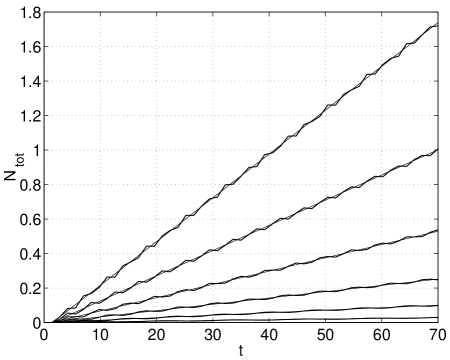
FIG. 3.: Total number of particles versus time for different frequencies of the oscillating mirror. The straight lines are linear fits to $N_{\rm tot}(t)$. The oscillation frequencies are of the form $\omega=n\pi/X_{0}$ with $n=4,6,8,10,12,14$. $60$ modes were used to calculate the total particle number.

It is clear from Fig. 3 that the evolution is effectively linear for the period shown. The production rate changes only for times of the order of twice the box length - up to then each oscillation produces roughly the same increase in particle number. This suggests that for small times, the field disturbances radiate away from the moving boundary without significant interference. For later times, after reflecting back on the stationary wall, they will interact with the vibrating mirror, constructively or otherwise depending on their frequency, leading to a change in the production rate.

For each value of the oscillating frequency $\omega$, we fitted the results to a linear law of the form $N_{\rm tot}(t)=\gamma t$. We checked that allowing for a constant term in the linear expression, $N_{\rm tot}(t)=b+\gamma t$ did not change the estimate for the production rate $\gamma$ ($b$ was always found to be very small, of order less than $10^{-3}$). Clearly, higher oscillating frequencies lead to higher particle production rates. In Fig. 4 the dependence of $\gamma$ on the mirror’s frequency is made more explicit. The results are very well fitted by a power law of the form $N_{\rm tot}(t)=D\,\omega^{k}\,t$ with $k=3.3$, a result in agreement with the analytical estimates in the literature. It is generally predicted that for a single oscillation the number of particles produced varies as a power law of the oscillation frequency. The particular value of the power depends on the specific type of oscillating trajectory. In [12] the production power for half an oscillation was shown to vary between $2.$ and $4.$, and in [13] a $\omega^{4}$ dependence was found in the limit of small velocities. For a single oscillation, our result corresponds to a power of $2.3$, which is in line with these values.

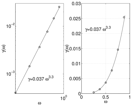
FIG. 4.: Fit of the particle production rate to a power law, log-log and linear scales.

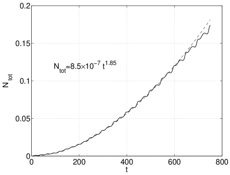
FIG. 5.: Total particle production versus time for the n=2 resonance frequency. The fit to a power law - dashed line - is for times varying from $t=100$ till $t=700$. 40 modes were used in the simulation.

As for the amplitude coefficient $D$, it was suggested in [13] that it should vary quadratically with the amplitude of the vibration of the mirror. We performed a quick test of this estimate by repeating the same set of runs with $A$, the mirror oscillating amplitude set to $1.$, half its previous value. Fitting both sets of data simultaneously to the same power $k$ and allowing $D$ to vary, we obtained $k=3.2$, $D=0.0342$ and $D=0.00780$ for $A=2.$ and $A=1.$ respectively. The rate of the two amplitudes is $0.23$, consistent with a reduction by a factor of $4$ as expected.

We now look at the longer time behaviour of the system. As mentioned above, the evolution stops being described by a linear law at about $t\simeq 2X_{0}$, when a new regime with a different production rate sets in. In Fig. 5 we can see the total particle number for longer times for the resonant frequency $\omega=2\pi/X_{0}$.

The evolution for the period of time shown is well fitted by a power law $N_{\rm tot}=8.5\times 10^{-7}t^{\alpha}$, with $\alpha=1.85$. For the dynamical range in question a power law growth with $\alpha=2.$ was predicted in ref. [4]. This is in reasonable agreement with our numerical estimate.

For higher frequencies, as far as we are aware, there are no explicit predictions for the particle number time dependency (see [18, 19] for a calculations of the energy produced). In Fig. 6 we show $N_{\rm tot}$ as a function of time for two higher resonant frequencies $\omega=6\pi/X_{0}$ and $\omega=7\pi/X_{0}$. We also include $N_{\rm tot}$ for the off-resonant case $\omega=6.5\,\pi/X_{0}$.

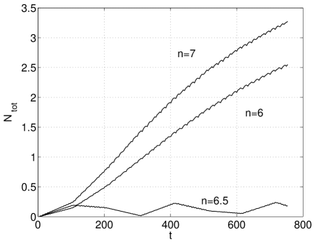
FIG. 6.: Total number of particles produced for resonant frequencies n=6 and n=7 and off-resonant frequency n=6.5. 40 modes used in the simulation.

The overall evolution does not fit any simple expression in any of the three cases. We note that the initial period of linear evolution is always present and we have checked that the production rates follow the power law shown in Fig. 4, even in the off-resonant case. For later times though, the contrast between off-resonant and resonant trajectories is very clear, with limited quasi-periodic production in the former case and continuing increase in the later. It is interesting not to find any qualitative difference between the long time behaviour of the even and odd resonant frequencies systems, n=6 and n=7. In fact it has been often suggested that the main phenomena governing the evolution in the long time limit is akin to parametric resonance [4]. If that were strictly the case though, resonant amplification would only take place for oscillating frequencies equal to twice the cavity’s natural frequencies [20]. That is, using our notation, we should see long time suppression of the production rate for odd values of $n$, which clearly is not the case. This seems to confirm the results in [19] where it was found that the energy produced grows exponentially for long times, for any motion with $\omega$ equal to a multiple of the fundamental frequency $\pi/X_{0}$.

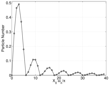
FIG. 7.: Particle spectrum for $\omega=6\pi/X_{0}$, $t=720$.

We now look at the distribution of the particles produced in terms of their frequency. In Fig. 7 we show the late time particle spectrum for the resonant $n=6$ motion. We observe an alternating succession of excited and suppressed frequencies. In particular we see that there is no production at all for frequencies multiple of the oscillating frequency. This cancellation is exact and it coincides strictly with points of the form $N\omega$, with $N$ integer. The peaks of the spectrum follow a similar but less precise pattern. The most excited frequency is $\omega/2$ and the following peaks take place at about points $M\omega+\omega/2$, though there seems to be a tendency for the peak to move up for higher frequencies. The fact that the maximum of the production rate corresponds to a frequency of about half the excitation, with higher even multiples suppressed and odd ones enhanced, is once again reminiscent of parametric resonance. Nevertheless, since the same pattern is observed for oscillating frequencies odd multiples of $\pi/X_{0}$, we must conclude that a more complex process is operating in the system.

Finally we contrast the resonant spectrum with the $n=6.5$ off-resonant case as shown in Fig. 8. Clearly, the overall amplitude is greatly reduced (by about one order of magnitude) and the pattern of alternating peaks is no longer present. The single peak is once again centred around $\omega/2$ but its height oscillates widely in time, leading to the periodic fluctuations in total particle number shown in Fig. 6.

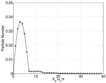
FIG. 8.: Particle spectrum for the off-resonant motion $\omega=6.5\pi/X_{0}$, for $t=720$.

IV Non-uniform time-varying Dielectric

In the examples discussed above, the varying geometry of the systems considered was the primary cause behind particle production from the initial vacuum state. In this Section we will look at a system with fixed dimensions, but whose bulk physical properties change both in space and in time. In particular we will consider wave propagation in a background with a space and time dependent dielectric “constant”. The system will be modelled by a straightforward generalisation of the wave equation [21]

$$\frac{\partial}{\partial t}\left(\epsilon(x,t)\frac{\partial\phi}{\partial t}\right)=\frac{\partial^{2}\phi}{\partial x^{2}},$$ (24)

where $\epsilon(x,t)$ is the varying dielectric term. Other generalisations are possible, their form depending ultimately on the properties of the particular system one chooses to model. In [22], the change in $\epsilon$ is caused by a moving half-infinite dielectric material, and compliance with Lorentz invariance leads to a wave equation with a cross derivative term. In so-called slow light experiments [7], based on electromagnetically-induced transparency, the optical properties of the medium are controlled by an external source. These systems can be described by an effective Lagrangian that includes a mass-like term for the field, leading to yet another choice of field theory. Here, for the sake of simplicity we follow [21] and use Eq. (24), though our approach can be easily extended to the cases mentioned above.

For two solutions of Eq. (24) the time invariant scalar product is given by

$$(\phi_{1},\phi_{2})=-i\int_{0}^{L}\epsilon(x,t)\left[\phi_{1}\,\partial_{t}\phi^{*}_{2}-\partial_{t}\phi_{1}\,\phi^{*}_{2}\right]\,dx$$ (25)

the fields being defined in a finite box of size $L$. We will look at cases where $\epsilon(x,t)$ is spatially uniform both for the initial and final times, $t_{1}$ and $t_{2}$. The corresponding normalised mode basis are given by:

$$u_{n}(x,t)=\sqrt{\frac{c_{i}}{n\pi}}e^{-i\omega_{n}t}\sin(k_{n}x),$$ (26)

$$\,\,\,\omega_{n}=c_{i}k_{n},\,\,\,\,k_{n}=\frac{n\pi}{L}\,\,\,\,\,\,\,\,n=1,\dots,\infty$$ (27)

where $c_{i}=1/\sqrt{\epsilon_{i}}$ with $i=1,2$ denotes the initial and final speed of light respectively.

In the specific scenario we will be simulating, the original medium with dielectric constant $\epsilon_{1}$ is replaced throughout the box by a medium characterised by $\epsilon_{2}$. Medium $1$ expands into medium $2$ from left to right with a given velocity $v$, as a one-dimensional analogue of an expanding bubble. At intermediate time steps, the two regions with different dielectric constants are separated by a “wall” that interpolates between $\epsilon_{1}$ and $\epsilon_{2}$. We model the wall profile as a sine

$$\chi(x)=\left\{\begin{array}[]{cl}\epsilon_{1},&\mbox{if $x>d/2$}\\ \epsilon_{+}-\epsilon_{-}\sin(\pi x/d),&\mbox{if $-d/2<x<d/2$}\\ \epsilon_{2},&\mbox{if $x<-d/2$}\end{array}\right.$$ (28)

with $\epsilon_{+}=(\epsilon_{1}+\epsilon_{2})/2$, $\epsilon_{-}=(\epsilon_{1}-\epsilon_{2})/2$, $d$ being the wall thickness. Using the wall profile $\chi(x)$ we can easily define a time-dependent dielectric function modelling the setting described above, as $\epsilon(x,t)=\chi(x-vt)$ with $t$ varying between $t_{1}=-d/(2\,v)$ and $t_{2}=d/(2\,v)+L/v$. We will be looking at cases where the final speed of light is less than the original one, corresponding to a vacuum box being filled with a denser medium. The initial dielectric constant will be set to $\epsilon_{1}=1$ with $\epsilon_{2}>\epsilon_{1}$. In general we will constrain the wall expansion velocity to be less than the speed of light in both the initial and final medium, that is $v<1/\sqrt{\epsilon_{2}}<1/\sqrt{\epsilon_{1}}$

In Fig. 9 we illustrate the dependence of the number of particles produced on the expansion velocity. The wall thickness was set to $d=5.$, considerably smaller than the physical box size, $L=50.$ The initial dielectric constant was fixed to $\epsilon_{1}=1.$ whereas its final value $\epsilon_{2}$ was varied between $1.2$ and $4.0$. For each particular choice of $\epsilon_{2}$ we simulated a series of expansion velocities ranging from $v\simeq 0.3$ up to the limit $v\simeq 1/\sqrt{\epsilon_{2}}$.

We found that for low velocities the production rate was considerably suppressed. As the expansion velocity increases, the total number of particles produced goes up steeply - on average by more than two orders of magnitude - as shown in Fig. 9. For mid and high values of the velocity, the dependence of the final particle number on $v$ is well described by an exponential law, $N_{\rm tot}=Ae^{\gamma v}$. This expression is valid up to values of $v$ considerably near the speed of light in the second medium.

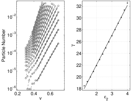
FIG. 9.: Left plot: particle number vs expansion velocity for values of $\epsilon_{2}$ varying between $1.2$ and $4.0$ (bottom to top curves). The data was fitted for medium and high-$v$ to an exponential $Ae^{\gamma v}$. The dependence of $\gamma$ on the final dielectric constant $\epsilon_{2}$ is shown in the right plot. The results are well fitted by a linear function $\gamma=\frac{K_{0}}{c_{1}}+\frac{K_{1}}{c_{1}}\frac{\epsilon_{2}}{\epsilon_{1}}$, with $K_{0}=12.0$ and $K_{1}=5.1$

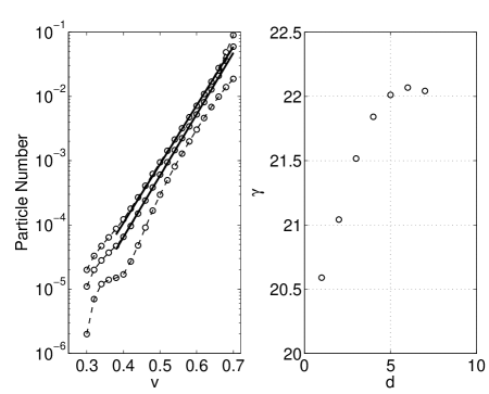
FIG. 10.: Left plot: particle number dependence on the expansion velocity, for three different values of the wall thickness $d=2,5,12$ (top to bottom). For the two lower values of $d$ we fitted the data to $N_{\rm tot}=Ae^{\gamma v}$. For the higher value of the thickness, the results no longer follow a simple exponential law. In the right plot we show $\gamma$ as a function of the wall thickness for $d$ varying between $1$ and $7$.

When the final dielectric constant is allowed to vary we observe as expected, that stronger changes in the optical properties of the system lead to higher production rates. As a consequence we should observe an increase in the coefficient $\gamma$ for higher values of $\epsilon_{2}$. This is fact the case, and it turns out that the dependence of $\gamma$ on the final dielectric constant is very simple. In the regime studied $\gamma$ varies linearly with $\epsilon_{2}$ as can be seen in the fit shown in the right plot of Fig. 9. Using dimensionality arguments we can then write

$$N_{\rm tot}\propto\exp\left[\left(K_{0}+K_{1}\frac{\epsilon_{2}}{\epsilon_{1}}\right)\frac{v}{c_{1}}\right]$$ (29)

where the dimensionless constants in the exponential are given by $K_{0}=12.0$ and $K_{1}=5.1$ for the system in question.

We also tested how the properties of the system depend on the thickness of the wall separating the two media. For a fixed value of the final dielectric constant $\epsilon_{2}=2.$ we allowed $d$ to vary. A sample of the results is shown in Fig. 10. As expected, for larger values of $d$ the transition between the initial and final media is smoother, and the production rate is lower. As before, for $d\leq 8$ the final particle number depends exponentially on the expansion velocity, though for higher values of the wall thickness we observe deviations from this simple law. In the “thin wall” regime, the exponent $\gamma$ varies very little with $d$, as can be seen in the right plot in Fig. 10. For $1\leq d\leq 7$ the change in $\gamma$ is less than 10%.

Finally we checked whether these results depend on the specific shape of the wall profile. We replaced the sin wall by one where a linear function interpolates between the two dielectric constants. We observed that the results were virtually unchanged.

V Conclusions

We have developed and tested the numerical techniques necessary to tackle the problem of particle production from a vacuum state in general scenarios. In particular, we have shown that the approach performs quite well when applied to cosmology, to the dynamical Casimir effect and to systems with complex optical properties. In some of these cases we were able to use the numerical data to obtain simple phenomenological laws. This illustrates the power of the method and shows how it can be used as a tool to approach problems for which there is little or no analytical information. The opportunities are many, as was mentioned in the bulk of the paper. In the context of the dynamical Casimir effect, the first obvious step will be to generalise this approach to higher dimensions, where little is known analytically. This poses no obvious numerical difficulty, in contrast to the analytical problems raised by the loss of conformal invariance. Extensions to general types of geometry and the inclusion of a mass term in the theory should also be within reach of the method. Optical systems in $2D$ and $3D$ with alternative Lagrangians, and realistic phase transitions can also be subject to the same techniques. Finally, we should stress that since in general we are able to compute the full set of Bogolugov coefficients, we do not have to restrict the initial state to be in the vacuum. Time evolution of multi-particle states such as thermal configurations, can be easily simulated within this framework.

A Numerical Algorithm for Moving Boundary Conditions

In all simulations discussed above the scalar field wave equation was solved using a straight-forward Leap Frog algorithm (see for example [23]). Only the case of the moving mirror (Section  III) requires more attention. For a box with time-dependent length, if the lattice spacing is kept constant, the number of points in the simulation domain must change and this may lead to large numerical errors.

The Leap Frog (LF) discretization of the wave equation Eq. (15) is

$$\Pi_{i,n+1/2}=\Pi_{i,n-1/2}+dt\,\nabla^{2}\phi\mid_{i,n}$$ (A1)

$$\phi_{i,n+1}=\phi_{i,n}+dt\,\Pi_{i,n+1/2},$$ (A2)

where $i$ is the spatial lattice index and $n$ the time step. As usual with LF-type algorithms, the field and its momentum are defined respectively on integer and half-integer time-steps. As before the coordinate of the moving boundary will be denoted by $X(t)$, and at each time-step its value will not necessarily lie exactly on one of the lattice spatial points. This discrepancy will have to be taken into account. In particular, as $X(t)$ increases new points will be introduced in the lattice and one must find a rule for assigning a field or momentum value to these.

Let us start with the case where the new lattice point $i+1$ lies in a half-integer time slice $n+1/2$, as depicted in Fig. 11.

FIG. 11.: Update algorithm for the moving boundary problem: integer $i$ denotes spatial lattice index and $n$ is the time-step. For higher accuracy, we define auxiliary sites in both space and time directions as the boundary’s trajectory - diagonal line - crosses the lattice. The separation between these and their adjacent integer lattice coordinates is denoted respectively, by $\alpha$ and $\beta$.

We start by differentiating in respect to time the boundary condition $\phi(X(t),t)=0$,

$$\frac{\partial\phi}{\partial x}\mid_{(X(t),t)}\dot{X}(t)+\Pi(X(t),t)=0$$ (A3)

This allows us to calculate the momentum at the boundary in terms of the spatial derivative of the field. Since the field vanishes at the boundary, we can approximate $\partial_{x}\phi$ at the point $(i+1,n+1/2)$ by $-(\phi_{i,n}+\phi_{i,n+1})/(2\,dx)$, using the fact that $\phi_{i,n+1}$ can be evaluated in advance. This leads to:

$$\Pi_{i+1,n+1/2}=\frac{\dot{X}_{n+1/2}}{2\,dx}(\phi_{i,n+1}+\phi_{i,n})$$ (A4)

Note however that here we implicitly assume that the boundary crosses the lattice at precisely the point $(i+1,n+1/2)$, which is not necessarily true. The above estimate can be improved by introducing an auxiliary fictitious lattice point $(i+1,n+1/2-\beta)$, the exact location where the mirror’s trajectory intersects the lattice. The time difference between the crossing and time-step $n+1/2$ is given by $\beta\,dt$ and can be evaluated by interpolating the boundary trajectory between steps $n$ and $n+1/2$. At the crossing point we have

$$\Pi_{i+1,n+1/2-\beta}=\frac{\dot{X}_{n+1/2}}{2\,dx}\left[(1-2\beta)\,\phi_{i,n+1}+(1+2\beta)\,\phi_{i,n}\right]$$ (A5)

Note that by setting $\beta=0$ we recover the previous estimate Eq. (A4). Using Eq. (A5) we can then update the field at time-step $n+1$ as

$$\phi_{i+1,n+1}=dt\,(1/2+\beta)\,\Pi_{i+1,n+1/2-\beta}$$ (A6)

The next momentum up-date, at $n+3/2$, will be calculated taking into account that boundary was placed at $(i+1,n+1/2-\beta)$.

This method is easily generalised to the situation where the newly introduced lattice point lies on a integer time slice $n+1$. We proceed in a similar way, defining an auxiliary momentum point at $(i+1,n+1/2-\beta)$, though in this case $\beta$ will be negative. The following updates proceed exactly in the same way as described in Eqs. (A5) and (A6).

When the trajectory of the mirror is such that no new points need to be introduced, we must still take some care when updating the fields near the boundary. In particular, the calculation of the second derivative term $\nabla^{2}\phi\mid_{i,n}$ in Eq. (A2) should reflect the fact that the boundary may lie between lattice sites. Referring again to Fig. 11 we define $\alpha$ as the distance in lattice units from point $(i,n)$ to the mirror. Since the field vanishes at the boundary we will have

$$\nabla^{2}\phi\mid_{i,n}=\frac{\alpha\phi_{i-1,n}-(1+\alpha)\phi_{i,n}}{\alpha\,dx^{2}}$$ (A7)

By setting $\alpha=1$, this expression reduces to the less accurate estimate for the second derivative, where the boundary’s position is identified with lattice point $i+1$.

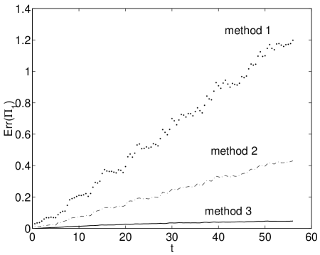
FIG. 12.: Numerical errors for three different methods for the first component of the momentum field $\Pi_{1}$. A single mode $\omega=n\pi/X_{0}$ with $n=16$ was evolved and compared with the corresponding analytical solution. The cavity expanded with constant velocity $v=0.9$ from initial size $X_{0}=50$.

In order to check the accuracy of the algorithm, we have used the exact analytical solution Eq. (22) for the uniformly expanding box and compared it to the corresponding numerical solution. In Fig.12 we show for a particular solution, the numerical errors for three different methods based on the approximations discussed above. The error is defined as the (normalised) integral of the square of the difference between the exact and numerical solutions. Algorithm $1$ is obtained by setting $\beta=0$ and $\alpha=1$ in Eqs. (A5) and (A7). This corresponds to a straight forward implementation of the Leap Frog method with no smoothing at the boundary in either time or space directions. Method $2$ includes the corrections for the momentum at the boundary but non-improved spatial derivatives ($\alpha=1$). Finally, in method $3$ both $\alpha$ and $\beta$ are evaluated at each time-step according to the mirrors’s position. The improvement in accuracy is clear: algorithm $3$ decreases the errors by a factor of $10$ over method $2$ and by a factor of $25$ over method $1$. For the purposes of the simulations in this work this is enough. Direct observation of the numerical solutions shows that the moving boundary introduces high-frequency discontinuities in the fields (in particular in the momentum). These are considerably reduced by method 3, and in the end they tend to average out when the Bogolugov coefficients are evaluated, leading to reasonably small errors in the final physical quantities.

REFERENCES

- [1] H. B. G. Casimir, Proc. Kon. Ned. Akad. Wet., 51, 793 (1948); K. A. Milton, The Casimir Effect: Physical Manifestations of Zero-Point Energy, (World Scientific Publishing Co., Singapore, 2001).
- [2] S. W. Hawking, Nature 248, 30 (1974); S. W. Hawking, Commun. Math. Phys., 43, 199 (1975).
- [3] N. D. Birrell and P. C. W. Davies, Quantum Fields in Curved Space, (Cambridge University Press, Cambridge, 1982).
- [4] V. V. Dodonov and A. B. Klimov, Phys. Rev. A53, 2664 (1996).
- [5] W. G. Unruh, Phys. Rev. Lett. 46, 1351 (1981).
- [6] Atificial Black Holes, edited by M. Novello, M. Visser and G. Volovik (World Scientific, Singapore, 2002).
- [7] U. Leonhardt, Nature 415, 406 (2002).
- [8] L. J. Garay, J. R. Anglin, J. I. Cirac and P. Zoller, Phys. Rev. Lett. 85, 4642 (2000).
- [9] R. Schützhold, G. Plunien and G. Soff, Phys. Rev. Lett. 88, 061101 (2002).
- [10] G. T. Moore, J. Mat. Phys. (NY) 9, 2679 (1970).
- [11] S. A. Fulling and P. C. W. Davies, Proc. R. Soc. London A348, 393 (1976).
- [12] M. Castagnino and R. Ferraro, Ann. Phys. (N.Y.) 154, 1 (1984).
- [13] S. Sarkar, in Photons and Quantum Fluctuations, eds. E. R. Pike and H. Walter, (Adam Hilger, Bristol, 1988).
- [14] V. V. Dodonov, A. B. Klimov and V. I. Man’ko, Phys. Lett. A149, 225 (1990).
- [15] C. K. Law, Phys. Rev. Lett. 74, 1931 (1994).
- [16] N. D. Antunes, in preparation.
- [17] see Martin Crocce, Diego A. R. Dalvit, Francisco D. Mazzitelli, quant-ph/0205104 and references therein.
- [18] C. Cole and W. Schieve, Phys. Rev. A52, 4405 (1995)
- [19] P. Wegryzn and T. Rog, Act. Phys. Pol. B32, 129 (2001).
- [20] L. D. Landau and E. M. Lifshitz, Mechanics - third edition, (Pergamon Press, Oxford, 2002).
- [21] C. K. Law, Phys. Rev. A49, 433 (1994).
- [22] G. Barton and C. Eberlein, Ann. Phys. (N.Y.) 227, 222 (1993).
- [23] W. H. Press, B. P. Flannery, S. A. Teukolsky and W. T. Vetterling, Numerical Recipes in C: The Art of Scientific Computing, (Cambridge University Press, Cambridge, 1990).