UB-ECM-PF 03/22
GUTPA 03/10/01

QCD phenomenology of static sources and gluonic excitations at short distances
Gunnar S. Bali
Department of Physics & Astronomy, The University of Glasgow, Glasgow G12 8QQ, Scotland
Antonio Pineda
Dept. d’Estructura i Constituents de la Matèria, U. Barcelona
Diagonal 647, E-08028 Barcelona, Catalonia, Spain

New lattice data for the $\Pi_{u}$ and $\Sigma_{u}^{-}$ potentials at short distances are presented. We compare perturbation theory to the lower static hybrid potentials and find good agreement at short distances, once the renormalon ambiguities are accounted for. We use the non-perturbatively determined continuum-limit static hybrid and ground state potentials at short distances to determine the gluelump energies. The result is consistent with an estimate obtained from the gluelump data at finite lattice spacings. For the lightest gluelump, we obtain $\Lambda_{B}^{\rm RS}(\nu_{f}=2.5\,r_{0}^{-1})=[2.25\pm 0.10({\rm latt.})\pm 0.21({\rm th.})\pm 0.08(\Lambda_{\overline{\rm MS}})]\,r_{0}^{-1}$ in the quenched approximation with $r_{0}^{-1}\approx 400$ MeV. We show that, to quote sensible numbers for the absolute values of the gluelump energies, it is necessary to handle the singularities of the singlet and octet potentials in the Borel plane. We propose to subtract the renormalons of the short-distance matching coefficients, the potentials in this case. For the singlet potential the leading renormalon is already known and related to that of the pole mass, for the octet potential a new renormalon appears, which we approximately evaluate. We also apply our methods to heavy light mesons in the static limit and from the lattice simulations available in the literature we obtain the quenched result $\overline{\Lambda}^{\rm RS}(\nu_{f}=2.5\,r_{0}^{-1})=\left[1.17\pm 0.08({\rm latt.})\pm 0.13({\rm th.})\pm 0.09(\Lambda_{\overline{\rm MS}})\right]\,r_{0}^{-1}$. We calculate $m_{b,\overline{\rm MS}}(m_{b,\overline{\rm MS}})$ and apply our methods to gluinonia whose dynamics are governed by the singlet potential between adjoint sources. We can exclude non-standard linear short-distance contributions to the static potentials, with good accuracy.
PACS numbers: 12.38.Bx, 12.38.Gc, 12.38.Cy, 12.39.Hg, 14.80.Ly, 14.65.Fy

1 Introduction

In recent years, we have witnessed growing interest in the physics of gluelumps and static hybrid potentials. In many cases this has been driven by increasingly reliable lattice simulations of their properties [1, 2, 3, 4, 5, 6, 7]. These results expose models of low energy QCD to stringent tests and therefore enhance our understanding of the underlying dynamics. The short distance physics of the static hybrid potentials is of particular importance. In this region, hybrids and gluelumps are intimately related and well suited to investigate the interplay between perturbative and non-perturbative physics. At short distances, $r$, one is faced with widely separated scales: $1/r\gg\Lambda_{\rm QCD}$. In such situations, effective field theories (EFTs) are particularly useful since they enable the physics associated with the different scales to be factorized in a very efficient and model independent way. One EFT designed to deal with the kinematical case of interest to us corresponds to potential non-relativistic QCD (pNRQCD) [8], in the static limit [9].

In Ref. [9] the gluelumps and the short distance regime of the static hybrids were studied within this EFT framework and general features identified. Some results known from the past [10, 5, 11, 12, 13] were recovered within a unified framework and in some cases extended.

One can go beyond this analysis and use lattice data plus the knowledge of the (perturbative) octet potential to obtain numerical values for gluelump masses in a particular scheme. However, analogously to the situation with the static singlet potential, the convergence of the perturbative series of the octet potential does not appear very promising. This is a general problem when different scales are factorized, and in particular perturbative from non-perturbative ones. The bad convergence is also related to the problem of factorizing non-perturbative quantities, without defining their perturbative counterparts [14], and is usually believed to be due to the existence of singularities in the Borel transform of the perturbative quantity. These singularities appear to be due to scales of order $e^{-n}\times$-(the typical scale of the perturbative quantity) in an $n$-loop calculation. In Ref. [15] one of the present authors proposed that, since these singularities are related to energy scales much lower than the ones that are supposedly included in the perturbative object, they should be subtracted from it and introduced in the matrix elements of the effective theory. This programme has been worked out for the pole mass and the static singlet potential [15, 16]. Here we apply the same approach to the static octet potential. This will allow us to determine absolute values for the gluelump masses from the spectrum of the static hybrids, as well as to study up to which scale one can use perturbation theory to describe hybrid potentials.

This paper is organized as follows. In Sec. 2 we will work out the rôle of gluelumps in pNRQCD, and how gluelumps and hybrid potentials are interrelated. In Sec. 3 we will then sketch how our lattice data have been obtained, before discussing and classifying renormalons and power corrections in the continuum $\overline{\rm MS}$ scheme as well as in a lattice scheme in Sec. 4. In the same section we will also generalise the renormalon subtracted ($\rm RS$) scheme of Ref. [15] to the case of the octet potential and discuss the scale dependence. In Sec. 5 we will obtain the gluelump masses in the $\rm RS$ scheme and relate these results to the lattice scheme. We will compare to previous literature and predict the gluelump spectrum. In Sec. 6 we will determine the binding energy of static-light mesons as well as the bottom mass, before we discuss generalisations to and relations with adjoint potentials, gluinonium and other objects with relevance to short-distance QCD in Sec. 7.

2 Hybrid potentials and gluelumps

We discuss the relationship between hybrid potentials and gluelumps at short distances. First we consider the EFT picture, before we discuss the symmetries that are relevant in the non-perturbative case. Finally we compare these expectations to lattice data.

2.1 pNRQCD and gluelumps

The pNRQCD Lagrangian at leading order in $1/m$ and in the multipole expansion reads [8, 9],

$$L_{\rm pNRQCD}=\int d^{3}\!{\bf r}\,d^{3}{\bf R}\,{\rm Tr}\,\Biggl{\{}{\rm S}^{\dagger}\left(i\partial_{0}-V_{s}\right){\rm S}+{\rm O}^{\dagger}\left(iD_{0}-V_{o}\right){\rm O}\Biggr{\}}-\int d^{3}{\bf R}{1\over 4}F_{\mu\nu}^{a}F^{\mu\nu\,a}+O(r).$$ (1)

All the gauge fields in Eq. (1) are evaluated in ${\bf R}$ and $t$, in particular $F^{\mu\nu\,a}\equiv F^{\mu\nu\,a}({\bf R},t)$ and $iD_{0}{\rm O}\equiv i\partial_{0}{\rm O}-g[A_{0}({\bf R},t),{\rm O}]$. The singlet and octet potentials $V_{i}$, $i=s,o$ are to be regarded as matching coefficients, which depend on the scale $\nu_{us}$ separating soft gluons from ultrasoft ones. In the static limit “soft” energies are of $O(1/r)$ and “ultrasoft” energies are of $O(\alpha_{\rm s}/r)$. Notice that the hard scale, $m$, plays no rôle in this limit. The only assumption made so far concerns the size of $r$, i.e. $1/r\gg\Lambda_{\rm QCD}$, such that the potentials can be computed in perturbation theory. Also note that throughout this paper we will adopt a Minkowski space-time notation.

The spectrum of the singlet state reads,

$$E_{s}(r)=2m_{\rm OS}+V_{s}(r)+O(r^{2})\,,$$ (2)

where $m_{\rm OS}$ denotes an on-shell (OS) mass. One would normally apply pNRQCD to quarkonia and in this case $m_{\rm OS}$ represents the heavy quark pole mass. For the static hybrids, the spectrum reads

$$E_{H}(r)=2m_{\rm OS}+V_{o}(r)+\Lambda_{H}^{\rm OS}+O(r^{2})\,,$$ (3)

where

$$\Lambda_{H}^{\rm OS}\equiv\lim_{T\to\infty}i\frac{\partial}{\partial T}\ln\langle H^{a}(T/2)\phi^{adj}_{ab}(T/2,-T/2)H^{b}(-T/2)\rangle\,,$$ (4)

$$\phi(T/2,-T/2)\equiv\phi(T/2,{\bf R},-T/2,{\bf R})={\rm P}\exp\left\{-ig\displaystyle\int_{-T/2}^{T/2}\!\!dt\,A_{0}({\bf R},t)\right\}\,,$$ (5)

and $H$ represents some gluonic field, for examples see Table 4 in Sec. 5.3.

Eq. (3) allows us to relate the energies of the static hybrids $E_{H}$ to the energies of the gluelumps,

$$\Lambda_{H}^{\rm OS}=\left[E_{H}(r)-E_{s}(r)\right]-\left[V_{o}(r)-V_{s}(r)\right]+O(r^{2}).$$ (6)

This equation encapsulates one of the central ideas of this paper. The combination $E_{H}-E_{s}$ is renormalon-free in perturbation theory [up to possible $O(r^{2})$ effects], and can be calculated unambiguously non-perturbatively: the ultraviolet (UV) renormalons related to the infrared (IR) renormalons of twice the pole mass cancel each other. However, $\Lambda_{H}$ contains an UV renormalon that corresponds to the leading IR renormalon of $V_{o}$.

The shapes (of some) of the $E_{H}(r)$ have been computed on the lattice for instance in Refs. [1, 2, 3, 4, 5, 6]. On the other hand the values of (some) $\Lambda_{H}$ have also been computed within a variety of models as well as in lattice simulations [12, 17]. Consistency would require that the values of $\Lambda_{H}$ obtained from $E_{H}-E_{s}$ and the values of $\Lambda_{H}$ directly obtained from gluelump computations should agree. This will be checked in Sec. 5.2 below.

Gluelump states are created by a static source in the octet (adjoint) representation attached to some gluonic content ($H$) such that the state becomes a singlet under gauge transformations. This is what would happen to heavy gluinos in the static approximation. Hence sometimes gluelumps are also referred to as gluinoballs or glueballinos in the literature. Without further information, their energy is only fixed up to a global constant. Only the energy splittings between different states have well defined continuum limits in lattice simulations. In lattice regularization at a lattice spacing $a$ the normalization ambiguity is reflected in a linear divergence $\propto a^{-1}$ while in dimensional regularization one encounters an UV renormalon. In the HQET picture of a heavy-light meson one faces a similar problem. In this situation one also has a static source (in the fundamental representation in this case), which has to be attached to some light-quark (and gluonic) content to become a singlet under gauge transformations. The binding energy ${\overline{\Lambda}}$ is again only defined up to a global constant [18] and only its sum with the pole mass is unambiguous:

$$M_{B}=m_{b,\rm OS}+{\overline{\Lambda}}^{\rm OS}+O(1/m_{b})\,.$$ (7)

We will investigate this situation in Sec. 6 below.

2.2 Symmetries of hybrid potentials and gluelumps

The spectrum of open QCD string states can be completely classified by the quantum numbers associated with the underlying symmetry group, up to radial excitations. In this case, these are the distance between the endpoints, the gauge group representation under which these endpoints transform (in what follows we consider the fundamental representation), and the symmetry group of cylindrical rotations with reflections $D_{\infty h}$. The irreducible representations of the latter group are conventionally labelled by the spin along the axis, $\Lambda$, where $\Sigma,\Pi,\Delta$ refer to $\Lambda=0,1,2$, respectively, with a subscript $\eta=g$ for gerade (even) $PC=+$ or $\eta=u$ for ungerade (odd) $PC=-$ transformation properties. All $\Lambda\geq 1$ representations are two-dimensional. The one-dimensional $\Sigma$ representations have, in addition to the $\eta$ quantum number, a $\sigma_{v}$ parity with respect to reflections on a plane that includes the two endpoints. This is reflected in an additional $\pm$ superscript. The state associated with the static singlet potential transforms according to the representation $\Sigma_{g}^{+}$ while the two lowest lying hybrid potentials are within the $\Pi_{u}$ and $\Sigma_{u}^{-}$ representations, respectively.

In contrast, point-like QCD states are characterised by the $J^{PC}$ of the usual $O(3)\otimes{\mathcal{C}}$ rotation group as well as by the gauge group representation of the source. In the pure gauge sector, gauge invariance requires this representation to have vanishing triality, such that the source can be screened to a singlet by the glue. States created by operators in the singlet representation are known as glueballs, octet states as gluelumps. In contrast to gluelump states, where the octet source propagates through the gluonic background, the normalization of glueball states with respect to the vacuum energy is unambiguous.

Since $D_{\infty h}\subset O(3)\otimes{\mathcal{C}}$, in the limit $r\rightarrow 0$ certain hybrid levels must become degenerate. For instance, in this limit, the $\Sigma_{u}^{-}$ state corresponds to a $J^{PC}=1^{+-}$ state with $J_{z}=0$ while the $\Pi_{u}$ doublet corresponds to its $J_{z}=\pm 1$ partners. The gauge transformation property of the hybrid potential creation operator will also change in this limit, ${\mathbf{3}}\otimes{\mathbf{3}^{*}}={\mathbf{1}}\oplus{\mathbf{8}}$, such that hybrids will either approach gluelumps [cf. Eq. (3)] or glueballs, in an appropriate normalization. In the case of glueballs the correct normalization can be obtained by considering the difference $E_{H}(r)-E_{s}(r)$ from which the pole mass cancels. We will discuss the situation with respect to gluelumps in detail in Sec. 4 below.

In perturbation theory, the ground state potential corresponds to the singlet potential while hybrid potentials will have the perturbative expansion of the octet potential.

Recently, Philipsen [19] suggested to non-perturbatively generalise the octet potential, employing a definition that resembles the perturbative one, after gauge fixing to Laplacian Coulomb gauge. He proved that this construction is equivalent to a gauge invariant correlation function whose eigenvalues will resemble masses of physical states. In the limit $r\rightarrow 0$ the suggested operator will be an adjoint temporal Schwinger line, dressed with a non-local but symmetric gluon cloud, with the $J^{PC}$ quantum numbers of the vacuum. A similar construction is mentioned in paragraph 2 of Sec. 6 below, as a possible non-perturbative normalization point for gluelump energies. The static “octet” potential suggested in Ref. [19] will have the $\Sigma_{g}^{+}$ symmetry and, up to a different non-perturbative off-set, the same perturbative expansion and power term/renormalon structure as the hybrid potentials discussed below. Due to the nature of its creation operator which is non-local, even in the $r=0$ limit, at present it is not obvious to us how this non-perturbative state can be interpreted in terms of the local states we are considering in this paper, certainly an open question that should be addressed in the future.

2.3 Hybrid and gluelump mass splittings

We would like to establish if lattice data on hybrid potentials reproduces the degeneracies expected from the above discussion in the short distance region. In the limit $r\rightarrow 0$, any given $\Lambda\geq 1$ hybrid potential can be subduced from any $J^{PC}$ state with $J\geq\Lambda$ and $PC=+$ for $\eta=g$ or $PC=-$ for $\eta=u$ representations. For instance the $\Pi_{u}$ is embedded in $1^{+-},1^{-+},2^{+-},2^{-+},\cdots$. The situation is somewhat different for $\Lambda=0$ states, which have the additional $\sigma_{v}$ parity: the $\Sigma_{g}^{+}$ representation can be obtained from $0^{++},1^{--},2^{++},\cdots$, $\Sigma_{g}^{-}$ from $0^{--},1^{++},\cdots$, $\Sigma_{u}^{+}$ from $0^{+-},1^{-+},\cdots$ and $\Sigma_{u}^{-}$ from $0^{-+},1^{+-},\cdots$. We list all combinations of interest to us in Table 1. The ordering of low lying gluelumps has been established in Ref. [12] and reads with increasing mass: $1^{+-},1^{--},2^{--},2^{+-},3^{+-},0^{++},4^{--},1^{-+}$, with a $3^{--}$ state in the region of the $4^{--}$ and $1^{-+}$. The $2^{+-}$ and $3^{+-}$ as well as the $4^{--}$ and $1^{-+}$ states are degenerate within present statistical uncertainties. The continuum limit gluelump masses are displayed as circles at the left of Fig. 1, where we have added the (arbitrary) overall constant $2.26/r_{0}$ to the gluelump splittings to match the hybrid potentials. The similarity of this value to our estimate of the gluelump energy in Sec. 5.1 below is purely accidental.

point particle $J^{PC}$	open string $\Lambda^{\sigma_{v}}_{\eta}$
$1^{+-}$	$\Sigma_{u}^{-},\Pi_{u}$
$1^{--}$	$\Sigma_{g}^{+\prime},\Pi_{g}$
$2^{--}$	$\Sigma_{g}^{-},\Pi_{g}^{\prime},\Delta_{g}$
$2^{+-}$	$\Sigma_{u}^{+},\Pi_{u}^{\prime},\Delta_{u}$
$3^{+-}$	$\Sigma_{u}^{-^{\prime}},\Pi_{u}^{\prime\prime},\Delta_{u}^{\prime},\Phi_{u}$
$0^{++}$	$\Sigma_{g}^{+\prime\prime}$
$4^{--}$	$\Sigma_{g}^{-\prime},\Pi_{g}^{\prime\prime},\Delta_{g}^{\prime},\Phi_{g},\Gamma_{g}$
$1^{-+}$	$\Sigma_{u}^{+\prime},\Pi_{u}^{\prime\prime\prime}$

Table 1: Expected degeneracies of hybrid potentials at short distance, based on the level ordering of the gluelump spectrum. Note that if the $3^{+-}$ gluelump turned out to be lighter than the $2^{+-}$ then the $\Sigma_{u}^{-^{\prime}},\Pi_{u}^{\prime},\Delta_{u},\Phi_{u}$ potentials would approach the $3^{+-}$ state while the $\Sigma_{u}^{+},\Pi_{u}^{\prime\prime},\Delta_{u}^{\prime}$ potentials would approach the $2^{+-}$ instead.

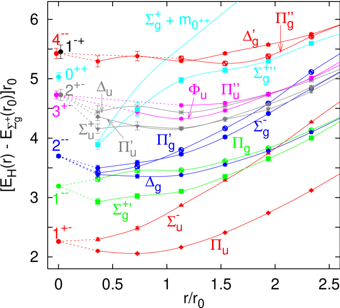
Figure 1: Different hybrid potentials [1] at a lattice spacing $a_{\sigma}\approx 0.2$ fm $\approx 0.4\,r_{0}$, where $r_{0}\approx 0.5$ fm, in comparison with the gluelump spectrum, extrapolated to the continuum limit [12] (circles, left-most data points). The gluelump spectrum has been shifted by an arbitrary constant to adjust the $1^{+-}$ state with the $\Pi_{u}$ and $\Sigma_{u}^{-}$ potentials at short distance. In addition, we include the sum of the ground state ($\Sigma_{g}^{+}$) potential and the scalar glueball mass $m_{0^{++}}$ [21, 22]. The lines are drawn to guide the eye.

Juge, Kuti and Morningstar [1] have, for the first time, comprehensively determined the spectrum of hybrid potentials. We convert their data, computed at their smallest lattice spacing $a_{\sigma}\approx 0.2$ fm, into units of $r_{0}\approx 0.5$ fm [20]. Since the results have been obtained with an improved action and on anisotropic lattices with $a_{\tau}\approx a_{\sigma}/4$, one might expect lattice artifacts to be small, at least for the lower lying potentials. Hence we compare these data, normalized to $E_{\Sigma_{g}^{+}}(r_{0})$, with the continuum expectations of the gluelumps [12]. The full lines are cubic splines to guide the eye while the dashed lines indicate the gluelumps towards which we would expect the respective potentials to converge.

The first 7 hybrid potentials are compatible with the degeneracies suggested by Table 1. The next state is trickier since it is not clear whether $2^{+-}$ or $3^{+-}$ is lighter. In the figure we depict the case for a light $2^{+-}$. This would mean that $(\Sigma_{u}^{+},\Pi_{u}^{\prime},\Delta_{u})$ approach the $2^{+-}$ while $(\Sigma_{u}^{-\prime},\Pi_{u}^{\prime\prime},\Delta_{u}^{\prime},\Phi_{u})$ approach the $3^{+-}$. Note that of the latter four potentials only data for $\Pi_{u}^{\prime\prime}$ and $\Phi_{u}$ are available. Also note that the continuum states $\Pi_{u}^{\prime},\Pi_{u}^{\prime\prime}$ and $\Phi_{u}$ are all obtained from the same $E_{u}$ lattice representation. For the purpose of the figure we make an arbitrary choice to distribute the former three states among the $E_{u}^{\prime},E_{u}^{\prime\prime}$ and $E_{u}^{\prime\prime\prime}$ lattice potentials. To firmly establish their ordering one would have to investigate radial excitations in additional lattice hybrid channels and/or clarify the gluelump spectrum in more detail. Should the $2^{+-}$ and $3^{+-}$ hybrid levels be inverted then $(\Sigma_{u}^{-\prime},\Pi_{u}^{\prime},\Delta_{u},\Phi_{u})$ will converge to the $3^{+-}$ while $(\Sigma_{u}^{+},\Pi_{u}^{\prime\prime},\Delta_{u}^{\prime})$ will approach the $2^{+-}$. We note that the ordering of the hybrid potentials, with a low $\Sigma_{u}^{+}$, makes the first interpretation more suggestive.

Finally the $\Sigma_{g}^{+\prime\prime}$ potential seems to head towards the $0^{++}$ gluelump but suddenly turns downward, approaching the (lighter) sum of ground state potential and scalar glueball [21, 22] instead. The latter type of decay will eventually happen for all lattice potentials but only at extremely short distances. We also remark that all potentials will diverge as $r\rightarrow 0$. This does not affect our comparison with the gluelump results, since we have normalized them to the $\Pi_{u}/\Sigma_{u}^{-}$ potentials at the shortest distance available. (The gluelump values are plotted at $r=0$ to simplify the figure.)

On a qualitative level the short-distance data are very consistent with the expected degeneracies. From the figure we see that at $r\approx 2\,r_{0}\approx 1\,$fm the spectrum of hybrid potentials displays the equi-distant band structure one would qualitatively expect from a string picture. Clearly this region, as well as the cross-over region to the short-distance behaviour $r_{0}<r<2\,r_{0}$, cannot be expected to be within the perturbative domain: at best one can possibly imagine perturbation theory to be valid for the left-most 2 data points. With the exception of the $\Pi_{u}$, $\Pi_{u}^{\prime}$ and $\Phi_{u}$ potentials there are also no clear signs for the onset of the short distance $1/r$ behaviour with a positive coefficient as expected from perturbation theory. Furthermore, most of the gaps within multiplets of hybrid potentials, that are to leading order indicative of the size of the non-perturbative $r^{2}$ term, are still quite significant, even at $r=0.4\,r_{0}$; for instance the difference between the $\Sigma_{u}^{-}$ and $\Pi_{u}$ potentials at this smallest distance is about 0.28 $r_{0}^{-1}\approx 110$ MeV.

2.4 The difference between the $\Pi_{u}$ and $\Sigma_{u}^{-}$ hybrids

From the above considerations it is clear that for a more quantitative study we need lattice data at shorter distances. In this paper we have obtained these for the lowest two gluonic excitations, $\Pi_{u}$ and $\Sigma_{u}^{-}$ (see Sec. 3). We display their differences in the continuum limit in Fig. 2. We see how these approach zero at small $r$, as expected from the short distance expansion. pNRQCD predicts that the next effects should be of $O(r^{2})$ (and renormalon-free). In fact, we can fit the lattice data rather well with a $\Delta E_{\Pi_{u}-\Sigma_{g}^{+}}=A_{\Pi_{u}-\Sigma_{u}^{-}}r^{2}$ ansatz for short distances, with slope (see Fig. 2),

$$A_{\Pi_{u}-\Sigma_{u}^{-}}=0.92^{+0.53}_{-0.52}\,r_{0}^{-3}\,,$$ (8)

where the error is purely statistical (lattice). This fit has been done using points $r{\ \lower-1.2pt\vbox{\hbox{\hbox to0.0pt{$<$\hss}\lower 6.0pt\vbox{\hbox{$\sim$}}}}\ }0.5\,r_{0}$. By increasing the fit range to $r{\ \lower-1.2pt\vbox{\hbox{\hbox to0.0pt{$<$\hss}\lower 6.0pt\vbox{\hbox{$\sim$}}}}\ }0.8\,r_{0}$ the following result is obtained,

$$A_{\Pi_{u}-\Sigma_{u}^{-}}=(0.83\pm 0.29)\,r_{0}^{-3}\,,$$ (9)

indicating stability of the result Eq. (8) above.

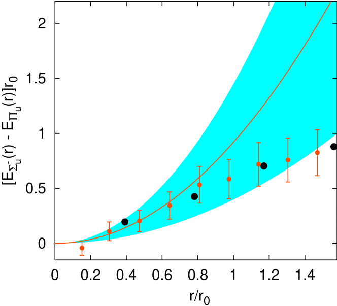
Figure 2: Splitting between the $\Sigma_{u}^{-}$ and the $\Pi_{u}$ potentials, extrapolated to the continuum limit, and the comparison with a quadratic fit to the $r{\ \lower-1.2pt\vbox{\hbox{\hbox to0.0pt{$<$\hss}\lower 6.0pt\vbox{\hbox{$\sim$}}}}\ }0.5\,r_{0}$ data points ($r_{0}^{-1}\approx 0.4$ GeV). The big circles correspond to the data of Juge et al. [1], obtained at finite lattice spacing $a_{\sigma}\approx 0.39\,r_{0}$. The errors in this case are smaller than the symbols.

In order to estimate systematic errors one can add a quartic term: $b\,r^{4}$ (only even powers of $r$ appear in the multipole expansion of this quantity). If the result is stable, our determination of $A_{\Pi_{u}-\Sigma_{u}^{-}}$ should not change much. Actually this is what happens. If we fit up to $r{\ \lower-1.2pt\vbox{\hbox{\hbox to0.0pt{$<$\hss}\lower 6.0pt\vbox{\hbox{$\sim$}}}}\ }0.5\,r_{0}$, we obtain the central value $A_{\Pi_{u}-\Sigma_{u}}r_{0}^{3}=0.93$ with a very small quartic coefficient, $b\,r_{0}^{5}=-0.05$. If we increase the range to $r{\ \lower-1.2pt\vbox{\hbox{\hbox to0.0pt{$<$\hss}\lower 6.0pt\vbox{\hbox{$\sim$}}}}\ }0.8\,r_{0}$, we obtain the same central value, $A_{\Pi_{u}-\Sigma_{u}^{-}}r_{0}^{3}=0.93$, but with a slightly bigger quartic term, $b\,r_{0}^{5}=-0.18$. Introducing the quartic term enhances the stability of $A_{\Pi_{u}-\Sigma_{u}^{-}}$ under variations of the fit range. From this discussion we conclude that the systematic error is negligible, in comparison to the error displayed in our result Eq. (8).

We remark that within the framework of static pNRQCD and to second order in the multipole expansion, one can relate the slope $A_{\Pi_{u}-\Sigma_{u}^{-}}$ to gluonic correlators of QCD.

3 Lattice determination of hybrid potentials

We extract the hybrid potentials in two sets of simulations, using the Wilson gauge action on an isotropic lattice with volume $24^{3}\times 48$ at $\beta=6.2$ ($a\approx 0.14\,r_{0}$) as well as on three anisotropic lattices with spatial lattice spacings $a_{\sigma}\approx 0.33,0.23,0.16\,r_{0}$, respectively, with anisotropy $a_{\sigma}\approx 4\,a_{\tau}$. The former result has been obtained in the context of the study of Ref. [4] (and has been published in Ref. [3]) while the simulation parameters, statistics and smearing of the latter runs are identical to those of Ref. [24]: $(\beta,\xi_{0})=(5.8,3.1),(6.0,3.2),(6.2,3.25)$. The isotropic data are used as a consistency check and in Sec. 4.4 below, while we extrapolate the data obtained on the anisotropic lattices to the continuum limit.

Some time was spent on improving the shape of the hybrid creation operators to optimize the overlap with the ground state [4]. The $\Pi_{u}$ potential has been determined on-axis as well as along a plane-diagonal, ${\mathbf{r}}/a_{\sigma}\propto(1,1,0)$, while the $\Sigma_{u}^{-}$ potential has only been obtained on-axis. Typically we achieved ground state overlaps of around 65 % for both potentials at $\beta=5.8$ and between 85 % and 90 % at the larger two $\beta$ values. Typical fit ranges for one-exponential fits to correlation functions for the $\Pi_{u}(\Sigma_{u}^{-})$ potential were $8\leq t/a_{\tau}\leq 18$, ($9\leq t/a_{\tau}\leq 14$) at $\beta=5.8$, $9\leq t/a_{\tau}\leq 24$ ($11\leq t/a_{\tau}\leq 21$) at $\beta=6.0$ and $13\leq t/a_{\tau}\leq 30$ ($15\leq t/a_{\tau}\leq 25$) at $\beta=6.2$. For all further details of the analysis we refer to Ref. [24] where potentials between sources in non-fundamental representations of $SU(3)$ were extracted using exactly the same methods.

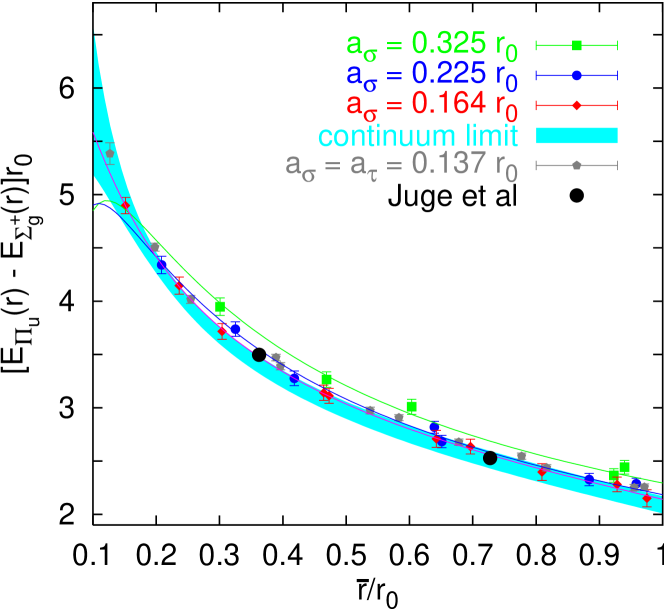
Figure 3: Continuum limit extrapolation of the difference between the $\Pi_{u}$ and the $\Sigma_{g}^{+}$ potentials vs. $\overline{r}=r[1+O(a^{2}/r^{2})]$ as described in the text [Eqs. (10) and (11)]. The Juge et al. data are from Ref. [1].

Subsequently, the potentials as well as differences between potentials have been extrapolated to the continuum limit. As one such example we display the difference between the $\Pi_{u}$ and the singlet potential in Fig. 3 for distances $r\leq r_{0}$. In this extrapolation we somewhat deviate from Ref. [24]: we follow Ref. [25] in removing the lattice artifacts to leading order in $\alpha_{s}$, by plotting the data as a function of the inverse lattice Coulomb propagator,

$$\overline{r}=a_{\sigma}\left[\frac{1}{{\mathbf{R}}}\right]_{L}^{-1}\,,$$ (10)

rather than of $r$. The lattice Coulomb propagator for the Wilson gauge action is given by,

$$\left[\frac{1}{{\mathbf{R}}}\right]_{L}=4\pi\int_{-\pi}^{\pi}\!\frac{d^{3}Q}{\left(2\pi\right)^{3}}\,\frac{\cos({\mathbf{Q}}{\mathbf{R}})}{4\sum_{i}\sin\left(\frac{Q_{i}}{2}\right)}\,,$$ (11)

and agrees with the continuum $1/R$-function up to $O(a^{2}/r^{2})$ lattice artifacts. ${\mathbf{R}}={\mathbf{r}}/a$ denotes an integer valued three-vector and the $Q_{i}=q_{i}a_{\sigma}$ are dimensionless. For the $\Pi_{u}$ potential this procedure removes violations of rotational symmetry within the statistical errors and brings the plane-diagonal points in-line with the on-axis data. Unfortunately, we cannot perform a similar internal test for the $\Sigma_{u}^{-}$ potential which we only determined for on-axis separations.

The next step involved fitting differences between hybrid potentials and $\Sigma_{g}^{+}$, $\Delta E_{H}=E_{H}-E_{\Sigma_{g}^{+}}$, for $r\geq 2a$ to the phenomenological interpolation,

$$\Delta E_{H}(r)=c_{1}+\frac{c_{2}+c_{3}\ln(r)}{r}+c_{4}r^{2}\,,$$ (12)

with parameters $c_{i}$. We then extrapolated these interpolating curves to the continuum limit, assuming the leading order $a_{\sigma}^{2}$ dependence. This was done separately for different pairs of two lattice spacings. The central value of the extrapolation is given by the result obtained from the $a_{\sigma}\approx 0.33\,r_{0}$ and $a_{\sigma}\approx 0.16\,r_{0}$ data sets. The error is estimated by the squared sum of the statistical error of the fine lattice data set and the difference between the above extrapolation and an extrapolation obtained from the $a_{\sigma}\approx 0.23\,r_{0}$ and $a_{\sigma}\approx 0.16\,r_{0}$ data sets. With decreasing $r$ the interpolating fits become less well constrained and hence the latter systematic uncertainty increases. The resulting error band is depicted in Fig. 3. Reassuringly, the $a_{\sigma}\approx 0.16\,r_{0}$ data are already in agreement with the continuum limit and the $a_{\sigma}\approx 0.23\,r_{0}$ data agree within errors: the fine lattice data set effectively already corresponds to the continuum limit. The more precise isotropic reference data ($a\approx 0.14\,r_{0}$) are also close to the continuum limit. We also notice that the first three data points of the coarse lattice data by Juge et al. [1] ($a_{\sigma}\approx 0.39\,r_{0}$) are compatible with our extrapolation. The same observations hold true for the $\Sigma_{u}^{-}$ potentials.

Rather than representing the continuum limit extrapolated potentials by error bands, in the remaining parts of this paper we add the difference between (finite $a$) interpolation and (continuum limit) extrapolation to the fine lattice data points and increase their errors by the systematic uncertainty involved in the extrapolation.

4 Static octet potential

We will discuss the octet potential in the OS ($=$ “pole mass”) scheme, compute the normalization constant of the renormalon and generalise the RS renormalon subtracted scheme [15] to this case. We will also discuss the structure of power divergences on the lattice and the analogous lattice scheme. Finally we discuss the running of the gluelump mass from one scale to another.

4.1 OS scheme for the octet potential

The octet potential in the case $1/r\gg\Lambda_{\rm QCD}$ can be computed order by order in perturbation theory. Nevertheless, it is not an IR safe object [26]. Its perturbative expansion reads,

$$V_{o}(r;\nu_{us})\simeq\sum_{n=0}^{\infty}V_{o,n}\alpha_{\rm s}^{n+1},$$ (13)

where we have made explicit its dependence on the IR cutoff $\nu_{us}$ and $\alpha_{\rm s}=\alpha_{\rm s}(\nu)$, where we define

$$\nu{d\alpha_{\rm s}\over d\nu}=-2\alpha_{\rm s}\left\{\beta_{0}{\alpha_{\rm s}\over 4\pi}+\beta_{1}\left({\alpha_{\rm s}\over 4\pi}\right)^{2}+\cdots\right\}.$$

In what follows we will always identify $\alpha_{s}$ with $\alpha_{\overline{\rm MS}}$. The first two coefficients $V_{o,0}$, $V_{o,1}$ are known, as well as the leading-log terms of $V_{o,3}$ [26] (for the renormalization-group improved expression see Ref. [27]). Note, however, that these leading logs are not associated to the first IR renormalon. For $V_{o,2}$ there exists a preliminary computation [28],

$$V_{o,2}=-{1\over N_{c}^{2}-1}V_{s,2}+\delta V_{o,2}\,,$$ (14)

$$\delta V_{o,2}\approx-{1\over 2N_{c}}{1\over(4\pi)^{2}}21C_{A}^{2}{1\over r}\,,$$ (15)

which we will use in what follows. $V_{s,2}$ has been computed in Ref. [29]. For $V_{o,3}$, we will use the renormalon-based estimate that we obtain in Sec. 4.2 below (Table 2).

b

Figure 4: $r_{0}V_{o}(r)$ (the octet potential in the OS scheme) at tree level (dashed lines), one-loop (dashed-dotted lines), two loops (dotted lines) and three loops (estimate) plus the leading single ultrasoft log (solid lines). Fig. a) corresponds to the scale $\nu=\nu_{i}$ [cf. Eq. (16)] and Fig. b) to $\nu=1/r$. In both cases, $\nu_{us}=2.5\,r_{0}^{-1}$. Only the solid curves depend on this choice.

Studying the convergence of perturbation theory of the octet potential in the OS scheme, conclusions similar to those in Ref. [16] are obtained. The poor convergence is demonstrated in Fig. 4, where we try two choices of the scale $\nu$. In part (a) we use $\nu=\nu_{i}$ where,

$$\nu_{i}={r^{\prime}}^{-1}=6.604\,r_{0}^{-1}\approx 2.6\,\mbox{GeV}\,,$$ (16)

corresponds to the shortest distance $r^{\prime}$ for which the continuum limit extrapolated lattice potentials are available. In part (b) we vary $\nu=1/r$. Obviously the curves depicted in the two parts of the figure agree with each other at $r=r^{\prime}\approx 0.15\,r_{0}$. Note the difference in the vertical scale.

4.2 Static octet potential normalization constant

We define the Borel transform of the octet potential as follows,

$$V_{o}=\int\limits_{0}^{\infty}\mbox{d}t\,e^{-t/\alpha_{\rm s}}\,B[V_{o}](t)\,,\qquad B[V_{o}](t)\equiv\sum_{n=0}^{\infty}V_{o,n}\frac{t^{n}}{n!}.$$ (17)

The behaviour of the perturbative expansion Eq. (13) at large orders is dictated by the closest singularity to the origin of its Borel transform, which happens to be located at $t=2\pi/\beta_{0}$. This singularity has two sources: one is an UV renormalon which cancels with the renormalon of twice the pole mass, the other is an IR renormalon that cancels with the UV renormalon of the gluelump energy. This result follows from the structure of the effective theory and the consequent factorization of the different scales in Eq. (3). Being more precise, the behaviour of the Borel transform of the static octet potential near the closest singularity to the origin [$u=1/2$ where we define $u=\beta_{0}t/(4\pi)$] reads,

$$B[V_{o}](t(u))=N_{V_{o}}\nu{1\over(1-2u)^{1+b}}\left(1+c_{1}(1-2u)+c_{2}(1-2u)^{2}+\cdots\right)+({\rm analytic\;term})\,,$$ (18)

where by analytic term, we mean a function that is analytic up to the next IR renormalon at $u=3/2$. This dictates the behaviour of the perturbative expansion at large orders to be,

$$V_{o,n}\stackrel{{\scriptstyle n\rightarrow\infty}}{{=}}N_{V_{o}}\,\nu\,\left({\beta_{0}\over 2\pi}\right)^{n}\,{\Gamma(n+1+b)\over\Gamma(1+b)}\left(1+\frac{b}{(n+b)}c_{1}+\frac{b(b-1)}{(n+b)(n+b-1)}c_{2}+\cdots\right).$$ (19)

The structure of the renormalon is equal to the singlet one. This is due to the fact that the number of octet fields is conserved at leading order in the multipole expansion and that the mass (potential) does not renormalize at this order. Therefore the values of the coefficients $b,c_{1},c_{2},\ldots$ above are the same as for the case of the static potential and the pole mass and can be found in Refs. [30, 31, 15]. We display them here for ease of reference:

$$b={\beta_{1}\over 2\beta_{0}^{2}}\,,$$ (20)

$$c_{1}={1\over 4\,b\beta_{0}^{3}}\left({\beta_{1}^{2}\over\beta_{0}}-\beta_{2}\right)\,,$$ (21)

and

$$c_{2}={1\over b(b-1)}{\beta_{1}^{4}+4\beta_{0}^{3}\beta_{1}\beta_{2}-2\beta_{0}\beta_{1}^{2}\beta_{2}+\beta_{0}^{2}(-2\beta_{1}^{3}+\beta_{2}^{2})-2\beta_{0}^{4}\beta_{3}\over 32\beta_{0}^{8}}\,.$$ (22)

The only difference with respect to the static singlet potential is the value of $N_{V_{o}}$. The cancellation of the renormalon in Eq. (3) requires,

$$2N_{m}+N_{V_{o}}+N_{\Lambda}=0\,,$$ (23)

where $N_{\Lambda}$ is the normalization constant of the renormalon of the gluelump mass ($B[\Lambda]$ reads the same as Eq. (18), with the replacement $N_{V_{o}}\mapsto N_{\Lambda}$). Therefore, unlike in the static singlet potential case, we cannot fix $N_{V_{o}}$ from the knowledge of $N_{m}$ alone. Yet we will (approximately) determine $N_{V_{o}}$ from low orders in perturbation theory of the octet potential. Note also that $N_{\Lambda}$ is independent of $H$, the specific gluonic content of the gluelump, since it only depends on the high energy behaviour, which is universal. To leading non-trivial order one obtains, $N_{V_{o}}=C_{A}/2-C_{f},N_{\Lambda}=C_{A}/2$.

In analogy to Refs. [32, 15, 16] we define the new function,

$$D_{V_{o}}(u) = \sum_{n=0}^{\infty}D_{V_{o}}^{(n)}u^{n}=(1-2u)^{1+b}B[V_{o}^{(0)}](t(u))$$

$$= N_{V_{o}}\nu\left(1+c_{1}(1-2u)+c_{2}(1-2u)^{2}+\cdots\right)+(1-2u)^{1+b}({\rm analytic\;term})\,,$$

and try to approximately determine $N_{V_{o}}$ by using the first three coefficients of this series. In analogy to Refs. [15, 16], we fix $\nu=1/r$ and obtain [up to $O(u^{3})|_{u=1/2}$],

$$N_{V_{o}}=0.166667-0.0624292+0.00976333=0.114001\,.$$ (25)

The convergence is rather good and, moreover, we have a sign alternating series. In fact, the scale dependence is becoming milder when we go to higher orders (see Fig. 5). Note that if the two loop coefficient $V_{o,2}$ had been equal to that of the singlet case [29] (with colour factor $C_{f}\mapsto C_{A}/2-C_{f}$), we would have obtained $N_{V_{o}}=0.146542$.

Figure 5: $x\equiv{\nu r}$ dependence of $N_{V_{o}}$ for $n_{f}=0$ at LO (dashed-dotted line), NLO (dotted line) and NNLO (dashed line).

We can now compute estimates for $V_{o,n}$ by using Eq. (19). These, as well as estimates for $V_{s,n}$, are displayed in Table 2 for $n_{f}=0$. We can see that the exact results are reasonably well reproduced. Hence we feel confident that we are near the asymptotic regime dominated by the first IR renormalon and that for higher $n$ our predictions will accurately approximate the exact results.

$$\begin{array}[]{|l||c|c|c|c|c|}\hline\cr{\tilde{V}}_{o,n}=rV_{o,n}&{\tilde{V}}_{o,0}&{\tilde{V}}_{o,1}&{\tilde{V}}_{o,2}&{\tilde{V}}_{o,3}&{\tilde{V}}_{o,4}\\ \hline\cr\hline\cr{\rm exact}\;(n_{f}=0)&0.166667&0.305472&1.27419&---&---\\ {\rm Eq.}\;(\ref{generalV})\;(n_{f}=0)&0.110552&0.244266&1.14193&6.97413&54.4562\\ \hline\cr\hline\cr{\tilde{V}}_{s,n}=rV_{s,n}&{\tilde{V}}_{s,0}&{\tilde{V}}_{s,1}&{\tilde{V}}_{s,2}&{\tilde{V}}_{s,3}&{\tilde{V}}_{s,4}\\ \hline\cr\hline\cr{\rm exact}\;(n_{f}=0)&-1.33333&-2.44378&-11.7893&---&---\\ {\rm estimate}\;(n_{f}=0)&-1.20643&-2.66564&-12.4616&-76.1075&-594.2718\\ \hline\cr\end{array}$$

Table 2: Values of $V_{o,n}$ with $\nu=1/r$: exact result (where available) and the estimate using Eq. (19). We also display the estimates of $V_{s,n}$ with $\nu=1/r$ (extracted from Ref. [15]).

In order to avoid large corrections from terms depending on $\nu_{us}$, the predictions should be understood with $\nu_{us}=1/r$ and later-on one can use the renormalization group equations for the static potential [27] to keep track of the $\nu_{us}$ dependence.

4.3 RS scheme for the octet potential

In Sec. 4.1 we have demonstrated the poor convergence of the perturbative expansion of the octet potential in the OS scheme. This bad behaviour is usually believed to be due to the singularities in the Borel transform of the perturbative expansion. Nevertheless, these singularities are fake since they cancel with singularities in the matrix elements. On the other hand this lack of convergence of perturbation theory arises because at higher orders in perturbation theory smaller and smaller momenta contribute to the short-distance matching coefficients of the effective theory. This clashes with the logic of scale separation in the EFT formalism. The solution advocated in Ref. [15] was to subtract this behaviour from the matching coefficients. At the practical level this was implemented by subtracting the Borel plane singularities of the matching coefficients. In Refs. [15, 16] this has been worked out for the pole mass and the static singlet potential and we refer to these references for the definitions and further details. In particular Eq. (2) reads,

$$E_{s}(r)=2m_{\rm RS}(\nu_{f})+V_{s,\rm RS}(r;\nu_{f})+O(r^{2})\,,$$ (26)

where

$$m_{\rm RS}(\nu_{f})=m_{\rm OS}-\delta m_{\rm RS}(\nu_{f})\,,$$ (27)

$$V_{s,\rm RS}(r;\nu_{f})=V_{s}(r)+2\delta m_{\rm RS}(\nu_{f})\,,$$ (28)

and (in the above equation we have already used the fact that the renormalon of the singlet potential cancels with the one of minus twice the pole mass),

$$\delta m_{\rm RS}(\nu_{f})=\sum_{n=1}^{\infty}N_{m}\,\nu_{f}\,\left({\beta_{0}\over 2\pi}\right)^{n}\alpha_{\rm s}^{n+1}(\nu_{f})\,\sum_{k=0}^{\infty}c_{k}{\Gamma(n+1+b-k)\over\Gamma(1+b-k)}\,.$$ (29)

Figure 6: $r_{0}V_{o,\rm RS}$ at tree level (dashed lines), one-loop (dashed-dotted lines), two loops (dotted lines) and three loops (estimate) plus the leading single ultrasoft log (solid lines). For the scale of $\alpha_{\rm s}(\nu)$, we set $\nu=\nu_{i}$ (stable behaviour at large distances) or $\nu=1/r$ (diverging at large distances). We kept $\nu_{f}=2.5\,r_{0}^{-1}$ fixed.

Figure 7: $r_{0}[V_{o,\rm RS}(r)-V_{o,\rm RS}(r^{\prime})]+C$ at tree level (dashed lines), one-loop (dashed-dotted lines), two loops (dotted lines) and three loops (estimate) plus the leading single ultrasoft log (solid lines) compared with the non-perturbative continuum-limit results for $E_{\Pi_{u}}(r)-E_{\Pi_{u}}(r^{\prime})$ (symbols with error bars). For the scale of $\alpha_{\rm s}(\nu)$, we set $\nu=\nu_{i}=1/r^{\prime}$ (stable behaviour at large distances) or $\nu=1/r$ (diverging at large distances). A (small) constant $C$ is arbitrarily adjusted to show agreement with the lattice data.

For the static hybrids, the spectrum reads,

$$E_{H}(r)=2m_{\rm RS}(\nu_{f})+V_{o,\rm RS}(r;\nu_{f})+\Lambda_{H}^{\rm RS}(\nu_{f})+O(r^{2})\,.$$ (30)

Obviously, we have to define the octet potential and the gluelump mass above. In the RS scheme the octet potential reads,

$$V_{o,\rm RS}(\nu_{f})=V_{o}-\delta V_{o,\rm RS}=\sum_{n=0}^{\infty}V^{\rm RS}_{o,n}\alpha_{\rm s}^{n+1}\,,$$ (31)

where

$$\delta V_{o,\rm RS}\equiv\sum_{n=1}^{\infty}N_{V_{o}}\,\nu_{f}\,\left({\beta_{0}\over 2\pi}\right)^{n}\alpha_{\rm s}^{n+1}(\nu_{f})\,\sum_{k=0}^{\infty}c_{k}{\Gamma(n+1+b-k)\over\Gamma(1+b-k)}\,.$$ (32)

This specifies the gluelump mass which reads,

$$\Lambda_{H}^{\rm RS}(\nu_{f})=\Lambda_{H}-\delta\Lambda_{\rm RS}(\nu_{f}),$$ (33)

where

$$\delta\Lambda_{\rm RS}(\nu_{f})=\sum_{n=1}^{\infty}N_{\Lambda_{H}}\,\nu_{f}\,\left({\beta_{0}\over 2\pi}\right)^{n}\alpha_{\rm s}^{n+1}(\nu_{f})\,\sum_{k=0}^{\infty}c_{k}{\Gamma(n+1+b-k)\over\Gamma(1+b-k)}\,.$$ (34)

Note that the potentials and $\Lambda_{H}^{\rm RS}$ depend on $\nu_{f}$ which, in the context of pNRQCD, can be thought of as a matching scale between ultrasoft and soft physics. In what follows, we will set $\nu_{f}=2.5\,r_{0}^{-1}$. Results for different values of $\nu_{f}$ can be obtained using the running on $\nu_{f}$, which is renormalon independent.

Analogously to the discussion of Ref. [16], we can study the convergence of the perturbative expansion in the RS scheme. In Fig. 6 we can see that the stability is greatly improved, compared to the OS scheme discussed in the previous section. No matter whether we choose to work with $\alpha_{\rm s}(\nu_{i})$ or $\alpha_{\rm s}(1/r)$, the expansions converge towards the same curve. In Fig. 7 we can also see that they agree with the continuum limit lattice data (we have to subtract an unknown constant for this comparison). In this figure the errors of $E_{\Pi_{u}}(r)-E_{\Pi_{u}}(r^{\prime})$ for $r>r^{\prime}$ are purely statistical while the (strongly correlated) systematic error of the continuum limit extrapolation is only displayed for the first data point [$E_{\Pi_{u}}(r^{\prime})-E_{\Pi_{u}}(r^{\prime})=0$], where it is largest.

The price we pay to obtain convergent expansions in $\alpha_{\rm s}$ for the potentials is the introduction of power-like terms (proportional to $\nu_{f}$, with logarithmic corrections). This behaviour very much resembles that of lattice regularization with a hard cut-off which we discuss below.

4.4 Lattice scheme for the octet potential

It is conceptionally illuminating also to consider the situation in lattice regularization. In this case, the inverse lattice spacing $a^{-1}$ results in a hard UV cut-off of the gluon momenta. Feynman diagrams are UV finite and EFT matrix elements are manifestly renormalon-free as long as they are obtained in non-perturbative numerical simulations. The price paid is the existence of power divergences $\propto a^{-1}$, which cannot be eliminated in the continuum limit.

The analogy with the previous sections can be made quite evident. In particular, all the quantities that we have defined in the OS and RS schemes can also be defined in a lattice scheme. There are some differences however. The lattice gluelump $\Lambda_{H}^{L}(a)$ has a power divergence to start with (which can be traded in for a renormalon ambiguity when subtracted in perturbation theory). In this sense it is similar to $\Lambda_{H}^{\rm RS}(\nu_{f})$. While formally many expressions resemble those of the RS case, $a^{-1}$ plays a slightly different rôle than $\nu_{f}$ that separates soft from ultrasoft scales since $a\ll r\ll\nu_{f}^{-1}$. Another difference is that at finite lattice spacings the potentials remain finite as $r\rightarrow 0$. In particular, we will see that gluelumps are the $r\rightarrow 0$ limits of hybrid potentials (at finite lattice spacing), in perturbation theory as well as non-perturbatively. This should not be surprising since the $r\rightarrow 0$ limit at finite lattice spacing corresponds to the situation $r\ll a$. This means that the ultraviolet cutoff $\sim a^{-1}$ is much smaller than $r^{-1}$ and that the dynamical degrees of freedom are only the ultrasoft ones. Actually, in this situation, $\nu_{f}$ and $1/a$ play an analogous rôle.

Let us illustrate the above by first considering perturbation theory, before discussing the scale separation and how the lattice scheme translates into other schemes, at finite lattice spacings as well as in the continuum limit.

For simplicity we will consider the Wilson discretization of the continuum action. In this case the “lattice Coulomb term” $[1/{\mathbf{R}}]_{L}$ takes the form Eq. (11). For instance one can calculate the finite value, $[1/{0}]_{L}=3.17\ldots$. Using this notation, one finds the lattice results,

$$V_{s,L}({\mathbf{r}};a) = -C_{f}\alpha_{L}a^{-1}\left[\frac{1}{\mathbf{R}}\right]_{L}\left[1+O(\alpha_{L})\right]+2\delta m_{\rm stat}^{L}(a)\,,$$ (35)

$$V_{o,L}({\mathbf{r}};a) = \left(\frac{C_{A}}{2}-C_{f}\right)\alpha_{L}a^{-1}\left[\frac{1}{\mathbf{R}}\right]_{L}\left[1+O(\alpha_{L})\right]+2\delta m_{\rm stat}^{L}(a)\,,$$ (36)

where the “self energy” is given by,

$$a\delta m_{\rm stat}^{L}(a) = \frac{C_{f}}{2}\alpha_{L}\left[\frac{1}{{0}}\right]_{L}+\cdots$$ (37)

$$= \frac{C_{f}}{2}\alpha_{L}\left(v_{1}+v_{2}\frac{\alpha_{L}}{4\pi}+v_{3}\frac{\alpha_{L}^{2}}{(4\pi)^{2}}+\cdots\right)\,.$$

Note that unlike in dimensional regularization, by using a hard cut-off, such power divergencies appear naturally as part of the perturbative expansion. Eqs. (35) and (36) are both known to $O(\alpha_{\rm s}^{2})$ and Eq. (35) (as well as the difference $V_{o}-V_{s}$) is also known approximately to $O(\alpha_{\rm s}^{3})$, up to $O(\alpha_{\rm s}^{3}a^{2}/r^{2})$ lattice corrections [33]. In pure gauge theory with Wilson action, the coefficients of the expansion of $\delta m^{L}_{\rm stat}$ read [34, 18, 33, 35],

$$v_{1} = 3.1759115\ldots,$$ (38)

$$v_{2} = 0.21003(5)\times 10^{3}\,,$$ (39)

$$v_{3} = 20.4(3)\times 10^{3}\,.$$ (40)

$\alpha_{L}=3/(2\pi\beta)$ denotes the lattice coupling at a scale $a^{-1}$ which can be translated into other schemes such as $\overline{MS}$ by means of a perturbative computation,

$$\alpha_{L}=\alpha_{\rm s}(a^{-1})\left[1-b_{1}\frac{\alpha_{\rm s}(a^{-1})}{4\pi}-\left(b_{2}-2b_{1}^{2}\right)\frac{\alpha_{\rm s}^{2}(a^{-1})}{(4\pi)^{2}}+\cdots\right]\,$$ (41)

with [36],

$$b_{1} \approx 73.93539066\ldots\,,$$ (42)

$$b_{2} \approx b_{1}^{2}+1388.1645\,.$$ (43)

Let us now consider the singlet case. We have,

$$E^{L}_{\Sigma_{g}^{+}}({\mathbf{r}};a)=V_{s,L}({\mathbf{r}};a)+\Lambda_{\rm QCD}\left[O(\Lambda_{\rm QCD}^{2}r^{2})+O(\Lambda_{\rm QCD}^{2}a^{2})+O(a^{2}/r^{2})\right]\,,$$ (44)

where $\Lambda_{\rm QCD}$ represents a generic non-perturbative scale like $r_{0}^{-1}$. The last two terms account for possible non-perturbative lattice artifacts, which vanish as $a\rightarrow 0$. From the quarkonium energy $E_{s}(r)$ at $r\gg a$, we can non-perturbatively obtain the heavy quark mass in a lattice scheme,

$$m_{L}(a)=\frac{1}{2}\left[E_{s}(r)-E_{\Sigma^{+}_{g}}^{L}({\mathbf{r}};a)\right]+O(a^{2}/r^{2})\,.\\$$ (45)

By redefining,

$$\overline{V}_{s,L}({\mathbf{r}};a)=V_{s,L}({\mathbf{r}};a)-2\delta m_{\rm stat}^{L}(a)\,,$$ (46)

we can then achieve formal correspondence to Eqs. (26) and (2), respectively:

$$E_{s}(r) = 2m_{L}(a)+V_{s,L}({\mathbf{r}};a)+O(r^{2})$$ (47)

$$= 2m_{OS}+\overline{V}_{s,L}({\mathbf{r}};a)+O(r^{2})\,,$$ (48)

where the above two equations are correct up to $O(\Lambda_{\rm QCD}^{2}a^{2})$ and $O(a^{2}/r^{2})$ lattice corrections.

We can relate the heavy quark mass in the lattice scheme to the OS scheme,

$$m_{L}(a)=m_{\rm OS}-\delta m_{\rm stat}^{L}(a)\,.$$ (49)

$\delta m_{\rm stat}^{L}(a)$ contains the same renormalon as $m_{\rm OS}$, such that Eq. (49) has good convergence properties when expanded in terms of $\alpha_{\rm s}$. $m_{L}(a)$ is proportional to $a^{-1}$, with logarithmic, as well as $O(a^{2})$ lattice corrections. One can convert $m_{L}(a)$ order by order in perturbation theory into say $m_{\overline{\rm MS}}(\nu)$, without renormalon ambiguity.

In the lattice scheme we also have $E^{L}_{\Sigma_{g}^{+}}(0;a)=V_{s,L}(0;a)=0$: the sources are “smeared out” on a scale $a$ since the gluon, due to the UV cut-off, cannot resolve structures smaller than the lattice spacing. Consequently, the Coulomb term does not diverge as $r\rightarrow 0$ but approaches a finite value in units of $a$. In perturbation theory, in the limit $r\rightarrow 0$, the lattice $[1/{\mathbf{R}}]_{L}$ term exactly cancels with $2\delta m_{\rm stat}^{L}$: the perturbative expansion of $V_{s,L}({\mathbf{r}};a)$, Eq. (35) above, does not contain the renormalon associated with the pole mass. Non-perturbatively, in the limit $r\rightarrow 0$ the Wilson loop becomes a time independent constant, such that $E^{L}_{\Sigma_{g}^{+}}(0;a)=0$ too. As $r>0$ the perturbative $V_{s,L}$ acquires a power term.

Next we consider the hybrid case. We can calculate the gluelump mass in perturbation theory,

$$a\delta\Lambda_{L}(a)=\frac{C_{A}}{2}\alpha_{L}\left[\frac{1}{{0}}\right]_{L}+\cdots=\frac{C_{A}}{2}\alpha_{L}\left(v_{1}+v_{2}\frac{\alpha_{L}}{4\pi}\right)+\cdots\,,$$ (50)

where $v_{1}$ and $v_{2}$ are the same as for the case of $\delta m_{\rm stat}^{L}$ and can be found in Eqs. (38) and (39) above. Note that the $O(\alpha_{s}^{3})$ term is expected to be different and is not known at present. However, $\Lambda_{H}$ is related to the difference between $V_{o}$ and $V_{s}$, such that any difference with respect to the $v_{3}$ of Eq. (40) above will be suppressed by a colour factor $1/N_{c}^{2}$.

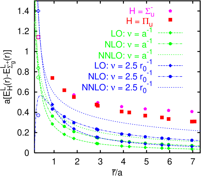
Figure 8: Splitting between the lowest two hybrids and the $\Sigma_{g}^{+}$ potentials (pentagons and squares) as a function of $\overline{r}/a$ [see Eq. (10)] at a fixed lattice spacing, $a\approx 0.137\,r_{0}$, in comparison to $V_{o,L}({\mathbf{r}};a)-V_{s,L}({\mathbf{r}};a)=\overline{V}_{o,L}({\mathbf{r}};a)-\overline{V}_{o,L}({\mathbf{r}};a)+\delta\Lambda_{L}(a)$ at tree level (dashed lines, diamonds), one loop (dashed-dotted lines, circles) and two loops (dotted lines, $r\gg a$ estimates). The open symbols correspond to the respective gluelumps, non-perturbatively (square with pentagon) and in lattice perturbation theory (diamonds and circles).

The tree level expression for $V_{o,L}$ is displayed in Eq. (36). While the perturbative expansion of $V_{s,L}$ was unaffected by the renormalon of the pole mass, the one of $V_{o,L}$ contains the same renormalon as the expansion of $\delta\Lambda_{L}$. For $r\gg a$ the renormalon-free combination $V_{o,L}({\mathbf{r}};a)-\delta\Lambda_{L}(a)$ plays the rôle of $V_{o,\rm RS}(r;\nu_{f})$ in Eq. (30). At $r=0$ we have, $V_{o,L}(0;a)=\delta\Lambda_{L}(a)$ as well as the non-perturbative equality,

$$E^{L}_{\Pi_{u}}(0;a)=E^{L}_{\Sigma_{u}^{-}}(0;a)=\Lambda_{B}^{L}(a)\,.$$ (51)

We redefine,

$$\overline{V}_{o,L}({\mathbf{r}};a)=V_{o,L}({\mathbf{r}};a)-\delta\Lambda_{L}(a)-2\delta m_{\rm stat}^{L}(a)\,,$$ (52)

to achieve formal correspondence with Eqs. (3) and (6):

$$E_{H}^{L}({\mathbf{r}};a)-E^{L}_{\Sigma_{g}^{+}}({\mathbf{r}};a)=\Lambda_{H}^{L}(a)+\left[\overline{V}_{o,L}({\mathbf{r}};a)-\overline{V}_{s,L}({\mathbf{r}};a)\right]+O(r^{2})\,.$$ (53)

Note that $E^{L}_{H}({\mathbf{r}};a)=E_{H}(r)-2m_{L}(a)+O(a^{2}/r^{2})$, in analogy to Eq. (45). The combination,

$$\overline{V}_{o,L}({\mathbf{r}};a)-\overline{V}_{s,L}({\mathbf{r}};a)=\frac{C_{A}}{2}\alpha_{L}a^{-1}\left(\left[\frac{1}{\mathbf{R}}\right]_{L}-\left[\frac{1}{{0}}\right]_{L}\right)+O(\alpha^{2})\,,$$ (54)

vanishes for $r=0$ and is renormalon-free. The same holds true for $E_{H}^{L}(0;a)-E_{\Sigma_{g}^{+}}^{L}(0;a)-\Lambda_{H}^{L}(a)=0$: Eq. (53) is not only valid for $r>a$ but also for $r=0$. We have,

$$\Lambda_{H}^{L}(a)=\Lambda_{H}^{\rm OS}+\delta\Lambda_{L}(a)\,.$$ (55)

Note that the above equation is only correct up to non-perturbative $O(\Lambda_{\rm QCD}^{2}a^{2})$ contributions to $\Lambda^{L}_{H}r_{0}$. Again $\Lambda_{H}^{L}$ is renormalon-free but has a power divergence. By subtracting $\delta\Lambda_{L}(a)$ order by order in perturbation theory one can obtain an on shell $\Lambda_{H}^{\rm OS}$, but at the price of a renormalon ambiguity. Note the similarity between the above equation and Eq. (33).

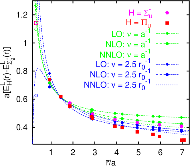
Figure 9: Splitting between the lowest two hybrids and the $\Sigma_{g}^{+}$ potentials (pentagons and squares) as a function of $\overline{r}/a$ [see Eq. (10)] at a fixed lattice spacing, $a\approx 0.137\,r_{0}$, in comparison with $\overline{V}_{o,L}({\mathbf{r}};a)-\overline{V}_{o,L}({\mathbf{r}};a)+C$ at tree level (dashed lines, diamonds), one loop (dashed-dotted lines, circles) and two loops (dotted lines, $r\gg a$ estimates). The vertical normalization $C$ has been adjusted to produce agreement at $r/a=\sqrt{2}$. The open symbols correspond to the respective gluelumps, non-perturbatively (square with pentagon) and in lattice perturbation theory (diamond and circles).

In Fig. 8 we compare non-perturbative data on the splitting between hybrid potentials with respect to the ground state potential with the perturbative expectation. The data have been obtained by us on an isotropic lattice at $\beta=6.2$ with lattice spacing $a\approx 0.137\,r_{0}$. Both gaps, $E^{L}_{\Pi_{u}}-E^{L}_{\Sigma_{g}^{+}}$ (squares) and $E^{L}_{\Sigma_{u}^{-}}-E^{L}_{\Sigma_{g}^{+}}$ (pentagons) are plotted as a function of $\overline{r}/a$ [see Eq. (10)]. The differences are indicative of the size of the expected non-perturbative $O(r^{2})$ contributions. We compare the non-perturbative data to the perturbative expectation for $V_{o,L}({\mathbf{r}};a)-V_{s,L}({\mathbf{r}};a)$. The latter perturbation theory will suffer from the same renormalon ambiguity as $\delta\Lambda_{L}(a)$ and the difference between perturbation theory and non-perturbative data corresponds to $\Lambda_{B}^{\rm OS}$. The left-most points (open symbols) correspond to the $\Lambda_{B}$ gluelump, plotted at $\overline{r}/a=[1/0]_{L}\approx 0.315$.

The evaluation was done both in terms of $\alpha_{s}(a^{-1})$ and $\alpha_{s}(\nu_{f})$ where $\nu_{f}=2.5\,r_{0}^{-1}\approx 0.34\,a^{-1}$. To simplify the figure we disregard the uncertainty in the determination of $\Lambda_{\overline{\rm MS}}=0.602(48)\,r_{0}^{-1}$ [37]. At LO and NLO lattice perturbation theory results are available [33] (diamonds and squares). Since everything is plotted as a function of $\overline{r}/a=[1/{\mathbf{R}}]_{L}^{-1}$ all diamonds lie exactly on top of the dashed continuous $r\gg a$ curves while at small distances there are differences between the dashed-dotted NLO curves and the exact NLO results (circles). In addition we plot the $r\gg a$ limits to NNLO (dotted curves). The shapes of the perturbative curves remain qualitatively stable while the normalization is not convergent as the order of the expansion is increased and is also strongly affected by the scale of $\alpha_{s}(\nu)$. This behaviour reflects the presence of the renormalon of $\Lambda_{B}^{\rm OS}$, quite similar to what we can see in Fig. 4a.

By comparing with the renormalon-free right hand side (rhs) of Eq. (53) a better convergence can be achieved. However, such a comparison is only possible up to $O(\alpha_{s}^{2})$ as we do not exactly know the $O(\alpha_{s}^{3})$ contribution to the counterterm $\delta\Lambda_{L}(a)$ in the lattice scheme. Instead we choose to demonstrate the quality of the perturbative expansion in Fig. 9 by adding global normalization constants to all curves in such a way that agreement is produced at $r/a=\sqrt{2}$. (We shall return to the question of renormalon cancellation in $\Lambda_{H}^{L}(a)$ in Sec. 5.2 below.) Indeed the differences between NNLO and NLO are smaller than those between NLO and LO. Moreover, at higher orders the scale dependence is reduced. The $\nu=a^{-1}$ curves seem to describe the data better at small $r$ while the $\nu=\nu_{f}$ curves seem to work better at larger $r$. Up to distances as big as $\overline{r}=r_{0}\approx 7.3\,a$ the perturbative curves seem to have an accuracy better than the non-perturbative uncertainties, estimated by the difference $E_{\Sigma_{u}^{-}}(r)-E_{\Pi_{u}}(r)$.

We mentioned above that while formally the lattice spacing $a^{-1}$ appears in the same places in the lattice scheme as the scale $\nu_{f}$ did in the RS scheme of Sec. 4.3, these two scales should not be confused with each other as $a^{-1}>r^{-1}>\nu_{f}>\Lambda_{\rm QCD}$. Conceptionally we have been discussing the situation in which the potentials are evaluated in perturbation theory at scales $\nu>\nu_{f}$ while $\Lambda_{H}^{\rm RS}$ is an ultrasoft matrix elements, associated to physics at scales smaller than $\nu_{f}$. The lattice encapsulates the same physical picture. For instance, to each finite order in perturbation theory, $V_{s/o,L}({\mathbf{r}};a)\stackrel{{\scriptstyle r\rightarrow\infty}}{{\longrightarrow}}2\delta m_{\rm stat}^{L}(a)$ and $V_{o,L}(0,a)=\delta\Lambda_{L}(a)$: the power contribution to the lattice mass $\delta m_{\rm stat}^{L}$ (whose perturbation theory is affected by the IR renormalon of the on shell mass) corresponds to the UV behaviour of the potentials while the power contribution to $\Lambda_{H}^{L}$ (whose perturbative expansion has the UV renormalon of $\Lambda_{H}^{\rm OS}$) is associated with the low energy behaviour of $V_{o,L}$. This is the same renormalon/power term structure as in the continuum OS/RS schemes.

For $a\ll r<\Lambda_{\rm QCD}^{-1}$ lattice effects become invisible and the formulae elaborated above apply under the replacement $\rm RS\mapsto L$. To illustrate this quasi-continuum limit, we eliminate the $a^{-1}$ dependence from the expressions altogether, which is straight forward:

$$E_{s}(r) = 2m_{L}(a)+E^{L}_{\Sigma_{g}^{+}}(r;a)\,,$$ (56)

$$= 2m_{L}(\nu_{f}^{-1})+V_{s,L}(r;\nu_{f}^{-1})+O(r^{2})\,,$$ (57)

where

$$V_{s,L}(r;\nu_{f}^{-1}) = V_{s,L}(r;a)-2\delta m_{\rm stat}^{L}(a)+2\delta m_{\rm stat}^{L}(\nu_{f}^{-1}),$$ (58)

$$m_{L}(\nu_{f}^{-1}) = m_{L}(a)+\delta m_{\rm stat}^{L}(a)-\delta m_{\rm stat}^{L}(\nu_{f}^{-1})\,.$$ (59)

Note that the running from one scale to another is renormalon-free. For the hybrid case we can directly write,

$$E_{H}(r)=2m_{L}(\nu_{f}^{-1})+[V_{o,L}(r;\nu_{f}^{-1})-\delta\Lambda_{L}(\nu_{f}^{-1})]+\Lambda_{H}(\nu_{f}^{-1})+O(r^{2})\,,$$ (60)

where the combination $V_{o,L}-\delta\Lambda_{L}$ replaces the $V_{o,RS}$ of Eq. (30).

Finally, we mention that the situation $r=0$ on the lattice resembles the $r\ll\nu_{f}^{-1}$ continuum situation. Unlike in the continuum, however, on the lattice, even at $r=0$, all observables remain finite as $a^{-1}$ provides us with a hard UV cut-off.

4.5 Scale dependence

As we have mentioned in the previous sections, the running of pole mass and gluelump energies with $\nu_{f}$, in the RS scheme, and with $a$, in the lattice scheme, is renormalon-free. Therefore, the functional dependence can be described by a convergent expansion in perturbation theory. Nevertheless, in order to achieve the renormalon cancellation, the same scale $\nu$ has to be used in the perturbative expansion. This produces large logs if the scales $\nu_{f}$ and $\nu_{f}^{\prime}$ are widely separated and, eventually, some errors, if one works to finite order in perturbation theory. In the RS scheme, there exists a solution to this problem. Even though $\delta m_{\rm RS}(\nu_{f})$ suffers from the renormalon ambiguity, the difference $\delta m_{\rm RS}(\nu_{f})-\delta m_{\rm RS}(\nu_{f}^{\prime})$ is renormalon-free. We can perform a resummation of $\delta m_{\rm RS}(\nu_{f})$ with any prescription to avoid the singularity in the Borel plane since it will cancel in the difference. We will take here the Principal Value (PV) prescription, which yields,

$$\delta m_{\rm RS}^{\rm PV}(\nu_{f})=N_{m}\nu_{f}\alpha_{\rm s}(\nu_{f})\sum_{s=0}^{\infty}c_{s}\left[D_{b-s}\left(-{2\pi\over\beta_{0}\alpha_{\rm s}}\right)-1\right]\,,$$ (61)

where

$$D_{b}(-x)=x\left\{e^{-x}(-x)^{b}\left[\Gamma(-b)-\Gamma(-b,-x)\right]-\cos(\pi b)e^{-x}\Gamma(-b)\right\}\,,$$ (62)

and,

$$\Gamma(b,x)=\int_{x}^{\infty}\!dt\,t^{b-1}e^{-t}\,,$$ (63)

denotes the incomplete $\Gamma$ function.

The second term in Eq. (62) corresponds to $\Lambda_{\overline{\rm MS}}$, once introduced in the sum of Eq. (61). It cancels from the combination, $\delta m_{\rm RS}^{\rm PV}(\nu_{f})-\delta m_{\rm RS}^{\rm PV}(\nu_{f}^{\prime})$, and we will not consider it any longer. The sum of Eq. (61) represents softer and softer singularities in the Borel plane. Therefore, we expect at least the difference $\delta m_{\rm RS}^{\rm PV}(\nu_{f})-\delta m_{\rm RS}^{\rm PV}(\nu_{f}^{\prime})$ to converge (although, obviously, we have no mathematical proof of this). Since the first three terms are known we can check if this actually happens. We can see that this is so with a high degree of confidence in Fig. 10.

Figure 10: $-\delta m_{\rm RS}^{\rm PV}(\nu_{f})+\delta m_{\rm RS}^{\rm PV}(\nu_{f}^{\prime})$ at LO (dashed line), NLO (dashed-dotted line) and NNLO (dotted line) according to the sum in Eq. (61). We take $\nu_{f}^{\prime}=9.76\,r_{0}^{-1}$.

We can also compare $-\delta m_{\rm RS}^{\rm PV}(\nu_{f})+\delta m_{\rm RS}^{\rm PV}(\nu_{f}^{\prime})$ with the corresponding difference, calculated at finite order in perturbation theory:

$$-\delta m_{\rm RS}(\nu_{f})+\delta m_{\rm RS}(\nu_{f}^{\prime})=-{\nu_{f}^{\prime}-\nu_{f}\over 2}{\tilde{V}}_{s,1}\alpha_{\rm s}^{2}(\nu)$$ (64)

$$\qquad\qquad-\left\{{\nu_{f}^{\prime}-\nu_{f}\over 2}{\tilde{V}}_{s,2}+\left[{\nu_{f}\over 2}{\beta_{0}\over\pi}\ln\left({\nu_{f}\over\nu}\right)-{\nu_{f}^{\prime}\over 2}{\beta_{0}\over\pi}\ln\left({\nu_{f}^{\prime}\over\nu}\right)\right]{\tilde{V}}_{s,1}\right\}\alpha_{\rm s}^{3}(\nu)+\cdots\,.$$

We depict this comparison in Fig. 11, where we take $\nu=\nu_{f}$ to minimise one of the logs. We see how the finite order results approach the PV curve, which we will use in what follows wherever we need the running.

Figure 11: $-\delta m_{\rm RS}(\nu_{f})+\delta m_{\rm RS}(\nu_{f}^{\prime})$ at LO (dashed line), NLO (dashed-dotted line) and NNLO (dotted line) in perturbation theory [see Eq. (64) with $\nu=\nu_{f}$) versus the Principal Value result (solid line). We take $\nu_{f}^{\prime}=9.76\,r_{0}^{-1}$.

A similar behaviour holds if, instead of $\delta m_{\rm RS}$, we study $\delta\Lambda_{\rm RS}$.

For the lattice scheme we cannot perform an analytical resummation as higher order terms are unknown. On the other hand, there exist non-perturbative lattice determinations of the static masses [$\Lambda_{H}^{L}(a)$ and ${\mathcal{E}}(a)=\overline{\Lambda}^{L}(a)$] for different lattice spacings. They provide us with non-perturbative measurements of the running against which the finite order results can be tested. It is also possible to relate results in both schemes by perturbative renormalon-free expressions. We will investigate both, the running within the lattice scheme and the translation between both schemes in Secs. 5.2 6.1 and 6.3 below.

5 Phenomenological analysis of the gluelump spectrum

We will determine the lowest gluelump energy, $\Lambda_{B}$, from two different observables in two different schemes: from the non-perturbative difference $E_{\Pi_{u}}(r)-E_{\Sigma_{g}^{+}}(r)$ in the continuum limit in the RS scheme as well as from gluelump energies $\Lambda_{B}^{L}(a)$ obtained at finite lattice spacings in a lattice scheme. Lattice and RS scheme can be translated into each other and we find internal consistency. We finally present results on the whole gluelump spectrum and compare our findings to previous literature.

The situation discussed here is similar to the one encountered in the “binding energy” in static-light systems which we will address in Sec. 6 below. These mesons very much resemble gluelumps, with the only difference that the source is in the fundamental representation and screened by a light quark rather than by a gluonic operator.

5.1 Determination of $\Lambda_{B}^{\rm RS}$ from the static potentials

We intend to determine $\Lambda_{B}$ from the hybrid potentials. For this purpose we will use our $n_{f}=0$ lattice continuum limit data on $\Delta E_{\Pi_{u}}(r)=E_{\Pi_{u}}(r)-E_{\Sigma_{g}^{+}}(r)$ as obtained in Sec. 3. Using this difference allows us to eliminate the power divergence that appears in lattice simulations of the potentials (or, in the continuum OS scheme, the renormalon associated with the pole mass). Note that the difference has a well defined continuum limit. It is also interesting to see that the large distance linear term is cancelled as well. At the same time, $\Lambda_{B}$ will still additively contribute to this combination, see Eq. (6). In order to extract this non-perturbative constant, the perturbative difference between octet and singlet potentials has to be subtracted. For a reliable determination, the perturbative series has to be well defined and show convergence. However, this is complicated by the contribution from the renormalon discussed above and can only be achieved in a scheme where such renormalon singularities are taken into account. We have worked out the RS scheme in Sec. 4.3, which is well suited for this purpose.

Figure 12: Splitting between the $\Pi_{u}$ and the $\Sigma_{g}^{+}$ potentials and the comparison with Eq. (65) for $\nu=\nu_{i}$ [see Eq. (16)] at $\nu_{f}=2.5\,r_{0}^{-1}$. $r_{0}[(V_{o,\rm RS}-V_{s,\rm RS})(r)+\Lambda_{B}^{\rm RS}]$ is plotted at tree level (dashed line), one-loop (dashed-dotted line), two loops (dotted line) and three loops (estimate) plus the leading single ultrasoft log (solid line).

Figure 13: Splitting between the $\Pi_{u}$ and the $\Sigma_{g}^{+}$ potentials and the comparison with Eq. (65) with $\nu=1/r$ for $\nu_{f}=2.5\,r_{0}^{-1}$. $r_{0}[(V_{o,\rm RS}-V_{s,\rm RS})(r)+\Lambda_{B}^{\rm RS}]$ is plotted versus r at tree level (dashed line), one-loop (dashed-dotted line), two-loops (dotted line) and three loops (estimate) plus the RG expression for the ultrasoft logs (solid line).

We fit $\Lambda_{B}$ using the following equality (see Figs. 12 and 13 for the quality of the fit):

$$E_{\Pi_{u}}(r)-E_{\Sigma_{g}^{+}}(r)=\Lambda_{B}^{\rm RS}(\nu_{f})+V_{o,\rm RS}(r;\nu_{f})-V_{s,\rm RS}(r;\nu_{f})\,,$$ (65)

where the non-perturbatively obtained left hand side (lhs) is renormalon-free but on the rhs the renormalon can be shifted between the two contributions, the ultrasoft matrix element $\Lambda_{B}$ and the soft Wilson coefficient $V_{o}-V_{s}$, at a given order of perturbation theory. This is why we have to specify the scheme, the RS scheme in our case, which we use to eliminate (or to reduce) this ambiguity.

We fix $\nu_{f}=2.5\,r_{0}$ and the final result reads,

$$\Lambda_{B}^{\rm RS}(\nu_{f}=2.5\,r_{0}^{-1})=\left[2.25\pm 0.10({\rm latt.})\pm 0.21({\rm th.})\pm 0.08(\Lambda_{\overline{\rm MS}})\right]\,r_{0}^{-1}\,.$$ (66)

Note that $\Lambda_{B}$ is the only fit parameter. Also note that the above value corresponds to the $n_{f}=0$ case. The errors of this determination stem from several sources (for the above fit we use lattice data up to distances of around 0.5 $r_{0}$):

1) “latt.” denotes the statistical error of the fit: $\pm 0.10$.

2) “th.” stands for the theoretical errors. We first consider the error due to the truncation of the perturbative series (higher orders in perturbation theory/scale dependence). We obtain a first estimate by performing the perturbative expansion in $\alpha_{\rm s}(\nu_{i})$ or in $\alpha_{\rm s}(1/r)$. This provides us with an estimate of neglected subleading logarithms. Actually, in both cases one and the same number, $\Lambda_{B}^{\rm RS}\approx 2.25\,r_{0}^{-1}$, is obtained, which we take as our central value. The effects of higher orders in perturbation theory are estimated by considering the convergence of the determination of $\Lambda_{B}^{\rm RS}$ at each order in perturbation theory. Working with $\alpha_{\rm s}(\nu_{i})$, the series $\{2.43,2.37,2.28,2.25\}$ is obtained. This series seems to show convergence for the last terms. In any case, the corrections are small. Working with $\alpha_{\rm s}(1/r)$, the series $\{2.00,2.40,2.31,2.25\}$ is obtained. This series is clearly convergent although the corrections are larger than when using $\alpha_{\rm s}(\nu_{i})$ as the expansion parameter. To be conservative we will take the difference between the last two terms as the error made by truncating the perturbative series: $\pm 0.06$. There is also some source of error from the normalization constant of the renormalon of the singlet and octet potential. For the singlet potential (following Ref. [15]) we estimate a $10\%$ error in $N_{V_{s}}$, which produces a $\pm 0.10$ error. For the octet potential, the error is very small compared with other sources of error. Even if, conservatively, we consider the general shift produced by setting $\delta V_{o,2}=0$ (note that this also accounts for the error in perturbation theory of the octet static potential) our result only changes by $\approx 0.01/0.02$. We will neglect this error to avoid double counting. In the above analysis we have neglected non-perturbative effects. On general grounds they have the structure

$$\delta_{np}(E_{\Pi_{u}}-E_{\Sigma_{g}^{+}})\simeq r^{2}F\left(V_{o}^{\rm RS}-V_{s}^{\rm RS}\over\Lambda_{\rm QCD}\right)+B\,r^{2}\,.$$ (67)

The $B\,r^{2}$ term is due to ${\bf r}\cdot O^{\dagger}{\bf E}O$ type contributions in the pNRQCD Lagrangian (see Ref. [9] for details). The other term in Eq. (67) is due to ${\bf r}\cdot O^{\dagger}{\bf E}S$ type contributions. This produces a perturbative mass gap. $F$ is the convolution of a short distance and a long distance piece, depending on the ratio of $V_{o}^{\rm RS}-V_{s}^{\rm RS}$ over the masses of the gluelumps. For the purpose of estimating the uncertainty it seems reasonable to keep the lowest order in this expansion. This is equivalent to having a quadratic contribution,

$$\delta_{np}(E_{\Pi_{u}}-E_{\Sigma_{g}^{+}})\simeq A_{\Pi_{u}-\Sigma_{g}^{+}}r^{2}\,.$$ (68)

If we introduce this term into the fit, we obtain $r_{0}\Lambda_{B}\approx 2.30$ [working with $\alpha_{\rm s}(1/r)$] with $A_{\Pi_{u}-\Sigma_{g}^{+}}\simeq-0.4\,r_{0}^{-3}$. We take the difference as an indication of the error due to non-perturbative effects. By summing linearly all the above errors we obtain $\pm 0.21$.

3) “$\Lambda_{\overline{\rm MS}}$”: this error is due to the uncertainty in $\Lambda_{\overline{\rm MS}}=[0.602\pm 0.48]\,r_{0}^{-1}$ [37]: $\pm 0.08$.

We have performed the fit using lattice data within a window of inverse distances ranging from about $\nu_{i}\approx 2.6$ GeV down to $\nu_{f}\approx~{}1$ GeV. From the plots (see Figs. 12 and 13) one can actually see that the curves follow the lattice data up to values $r{\ \lower-1.2pt\vbox{\hbox{\hbox to0.0pt{$<$\hss}\lower 6.0pt\vbox{\hbox{$\sim$}}}}\ }r_{0}$. This corresponds to very low energies ($<500$ MeV). Being conservative, we will not use data determined at these low energies without a better understanding of the dynamics. Nonetheless, such a fit would actually produce very similar numbers to the ones quoted above. This is even more so if a quadratic term is included. In general, introducing more lattice points reduces the statistical errors (“latt.”). Including a quadratic term will reduce the theoretical error on $\Lambda_{B}$ since some of the changes that occur when altering the order of perturbation theory can be absorbed into a variation of $A_{\Pi_{u}-\Sigma_{g}^{+}}$. However, the addition of a second fit parameter increases the statistical error and also the uncertainty due to $\Lambda_{\overline{\rm MS}}$. We conclude that while the individual errors depend on the precise fitting details the total error remains remarkably stable.

One might ask whether, in addition to $\Lambda_{B}$, a reliable value of $A_{\Pi_{u}-\Sigma_{g}^{+}}$ can be obtained. This however would require more lattice data at short distances as well as a more detailed understanding of the $r^{2}$ renormalon of the static singlet potential.

We do not consider the $\Sigma_{u}^{-}$ data in this section as we have already established in Sec. 2.4 above that the difference with respect to the $\Pi_{u}$ potential is proportional to $r^{2}$ to leading order. Hence we cannot obtain any independent new information on $\Lambda_{B}$ from these data, that have larger statistical errors.

5.2 Determination of $\Lambda_{B}^{\rm RS}$ from $\Lambda_{B}^{L}$

There exists a direct determination of $\Lambda_{B}^{L}(a)$ (the $1^{+-}$ or $B$ gluelump) by Foster and Michael [12]. The numerical values are displayed in Table 3, where we used the same $r_{0}/a$ values as were used in this reference. It is clear from the discussion in Sec. 4.4 that these are perfectly sensible numbers if incorporated into a global scheme with renormalon cancellation, for instance, with the potentials also defined in the lattice scheme as in Sec. 4.4. In doing this we are able to independently determine $\Lambda_{B}$ in a different scheme. Consistency would require that after translating the lattice into the RS scheme the results should agree with each other. We will check this in this section.

$a^{-1}r_{0}$	$\Lambda_{B}^{L}r_{0}/\Lambda_{B}^{\rm RS}r_{0}$(LO)	$\Lambda_{B}^{\rm RS}r_{0}$(NLO)	$\Lambda_{B}^{\rm RS}r_{0}$(NNLO)	$\Lambda_{B}^{\rm RS}r_{0}$(NNNLO*)	$\Lambda_{B}^{\rm RS}r_{0}$
2.94	5.33(10)	1.59(19)	2.82(12)	2.37(15)	2.41(10)
5.27	6.99(05)	1.97(17)	3.20(10)	2.88(12)	2.89(13)
7.32	8.36(05)	2.21(17)	3.55(10)	3.25(13)	3.16(13)

Table 3: The inverse lattice spacing, the mass of the $1^{+-}$ gluelump $\Lambda_{B}^{L}$ in the lattice scheme, as well as its conversion to the RS scheme to different orders in perturbation theory. NNNLO* stands for an estimate obtained neglecting $1/N_{c}^{2}$ corrections, for details see the text. In the last column, we state the values of $\Lambda_{B}^{\rm RS}(a^{-1})$ using Eq. (66) and the running according to the PV prescription, Eq. (61). The errors only incorporate the statistical uncertainties as well as the 8 % uncertainty in $\Lambda_{\overline{MS}}r_{0}$, added in quadrature, but no estimates of “theoretical” errors.

The master formula that relates the lattice and the RS scheme reads (known up to NNLO),

$$\Lambda_{H}^{\rm RS}(\nu_{f})=\Lambda_{H}^{L}(a)-\left[\delta\Lambda_{H}^{L}(a)+\delta\Lambda_{H}^{\rm RS}(\nu_{f})\right]\,.$$ (69)

Both, $\Lambda_{H}^{\rm RS}$ and $\Lambda_{H}^{L}$ have a power-like dependency on $\nu_{f}$ and $a^{-1}$, respectively, but are renormalon-free, $\Lambda_{H}^{L}$ exactly and $\Lambda_{H}^{\rm RS}$ within the precision of our estimation of the renormalon contribution. This implies that the combination $\delta\Lambda_{L}+\delta\Lambda_{\rm RS}$ does not contain a renormalon either if calculated in a consistent way: $\delta\Lambda_{L}(a)$ and $\delta\Lambda^{\rm RS}(\nu_{f})$ contain one and the very same renormalon contribution (with negative relative sign). The sum of both terms, expanded in terms of $\alpha_{\rm s}$ has good convergence properties (using the same normalization point to enforce the renormalon cancellation at each order in perturbation theory). The explicit expression at NNLO reads,

$$\delta\Lambda_{L}(a)+\delta\Lambda^{\rm RS}(\nu_{f})=\frac{C_{A}}{2}v_{1}a^{-1}\alpha_{\rm s}(\nu)$$ (70)

$$\qquad+\left\{\frac{C_{A}}{2}\frac{a^{-1}}{4\pi}\left\{v_{2}+v_{1}\left[-b_{1}+2\beta_{0}\ln(\nu a)\right]\right\}+\nu_{f}\left({\tilde{V}}_{s,1}-{\tilde{V}}_{o,1}\right)\right\}\alpha_{\rm s}^{2}(\nu)+\cdots\,,$$

where the $v_{i}$ can be found in Eqs. (38) and (39), $b_{1}$ in Eq. (42) and ${\tilde{V}}_{o,1}$ and $\tilde{V}_{s,1}$ in Table 2. An estimate of the $O(\alpha_{\rm s}^{3})$ term can be obtained from Eq. (6.1) below, under the replacements, $C_{f}\mapsto C_{A}$ and $\tilde{V}_{s,i}\mapsto 2(\tilde{V}_{s,i}-\tilde{V}_{o,i})$. This estimate will be subject to $O(1/N_{c}^{2})$ corrections to the coefficient $v_{3}$.

In principle, $\nu_{f}$ and $a^{-1}$ need not be equal but we will take them similar to avoid large logs. The large numerical values of $v_{2}$ and $b_{1}$ are mainly due to contributions from lattice-specific tadpole diagrams that arise because the breaking of Lorentz symmetry becomes particularly evident at UV scales $\simeq a^{-1}$. This often results in badly convergent perturbative series when expanded in terms of $\alpha_{L}(a)$. However, the convergence is vastly improved, once the series is re-expressed in terms of a more “physical” coupling like $\alpha_{s}(a^{-1})=\alpha_{L}[1-b_{1}\alpha_{L}^{2}/(4\pi)+\cdots]$ (see e.g. Refs. [33, 38]). This is also evident from Eq. (70) above as $v_{1}\approx 3.17$, $(v_{2}-b_{1}v_{1})/(4\pi)\approx-1.97$ [and $[v_{3}-2b_{1}v_{2}-(b_{2}-2b_{1}^{2})v_{1}]/(4\pi)^{2}\approx 14.5$].

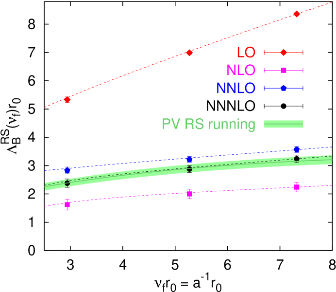
Figure 14: The lowest gluelump mass $\Lambda_{B}^{L}$ as obtained on the lattice (diamonds), as well as converted into the RS scheme at NLO (squares), NNLO (pentagons) and NNNLO* (NNNLO estimate, circles). The error band corresponds to the result for $\Lambda_{B}^{\rm RS}$ of Eq. (66), without the “theoretical” error, run to different scales, according to the PV prescription Eq. (61). The dashed lines, drawn to guide the eye, are explained in the text.

We can now translate the $\Lambda_{B}^{L}$ values obtained by Foster and Michael [12] into the RS scheme. The results are shown in Table 3 and are also displayed in Fig. 14. “NLO” and “NNLO” refer to translating from the lattice scheme to the RS scheme via Eq. (70) to $O(\alpha_{\rm s})$ and $O(\alpha_{\rm s}^{2})$, respectively. Obviously, to leading order, $\Lambda_{B}$ is scheme independent. “NNNLO*” stand for an estimate obtained assuming that the NNNLO contribution to $\delta\Lambda_{L}$ is equal to the NNNLO contribution to $\delta m^{L}$ with the replacement of the overall factor $C_{f}\mapsto C_{A}$. This is correct up to $O(1/N_{c}^{2})$ effects. Finally, the conversion from the lattice to the RS scheme has been performed using the 4-loop running of $\alpha_{\rm s}$ at $\nu=a^{-1}=\nu_{f}$. This accelerates the convergence to the RS results. If, instead, we use the $n$-loop running of $\alpha_{\rm s}$ that is consistent with the order of the calculation, we still see convergence but with, in the NLO and NNLO cases, larger corrections. This is mainly due to the fact that within the present window of energies the values obtained for $\alpha_{\rm s}(\nu)$ from $\Lambda_{\overline{\rm MS}}$ from a one- or two-loop running are significantly different from those from the three-loop running (which is close to four-loop). The lattice prediction of $\Lambda_{\overline{\rm MS}}$ that we use as an input applies to very high energies, such that it is important to run $\alpha_{\rm s}$ down to $\nu\geq 2.5\,r_{0}^{-1}$ as precisely as possible.

Within present errors we can fit the data with straight lines but there will be logarithmic corrections and, in the gluelump data $\Lambda_{B}^{L}r_{0}$, additional $O(a^{2})=O(\nu_{f}^{-2})$ lattice artifacts. The figure reveals that at the lattice spacings investigated these are tiny, relative to the linear slope. Except for these lattice corrections the running of $\Lambda_{B}^{L}$ is non-perturbatively accurate. Needless to say that the power dependence on $a^{-1}$ is universal for all gluelumps, such that gluelump mass splittings have a well defined continuum limit, which is also confirmed in Ref. [12].

In lattice perturbation theory we can calculate the “running” of the gluelump data to $O(\alpha_{\rm s}^{2})$ [and up to $O(\alpha_{\rm s}^{3})$ if we neglect $O(1/N_{c}^{2})$ effects]. There is a renormalon ambiguity in the absolute value. However the slope is not affected by this. If we take the value $\Lambda_{H}^{L}(7.32\,r_{0}^{-1})\approx 8.36\,r_{0}^{-1}$ from Table 3 and perform the running with NNNLO* accuracy, we obtain the dashed line that joins the “LO” $\rm RS(=L)$ points. We can see that this parametrization is quite close to the non-perturbatively evaluated data. Moreover, there is overall convergence, with higher order terms being numerically smaller in the lattice scheme. We will discuss this in more detail in Sec. 6 below, in the context of the static-light binding energy $\overline{\Lambda}^{L}$, which has a similar perturbative expansion, up to an overall factor $C_{f}/C_{A}$, see Fig. 15.

In Fig. 14 we also compare the value obtained in Sec. 5.1 above [Eq. (66)], with running according to the PV prescription Eq. (61), with the results obtained directly from the lattice determination of the gluelump mass via Eq. (70). We see clear convergence with alternating signs from LO (diamonds), NLO (squares), NNLO (pentagons) and NNNLO* (circles) towards the result calculated from the $\Pi_{u}$ and $\Sigma_{g}^{+}$ potentials in the previous section and its running (error band). Our NNNLO* estimates already agree with this error band. The dashed lines connecting the NLO, NNLO and NNNLO* points are the corresponding transformations of the curve through the LO points and just drawn to guide the eye. All errors displayed in Fig. 14 are statistical only, plus the uncertainty on $\Lambda_{\overline{\rm MS}}$. Within the theoretical errors of Eq. (66) ($\pm 0.21\,r_{0}^{-1}$), in fact we already find agreement at the NNLO level. In Secs. 6.1 and in particular 6.3 below we will analyse the running of the binding energy of static-light mesons in more detail, see also Fig. 18.

We obtain an independent second prediction for $\Lambda_{B}^{\rm RS}$ from the gluelump data. The statistical errors are smaller in the gluelump case than those we encountered from the continuum potentials. In a first step we obtain the fit parameter,

$$\Lambda_{B}^{\rm RS}(7.32\,r_{0}^{-1})=[3.21\pm 0.04(\mbox{latt.})\pm 0.42(\mbox{th.})\pm 0.10(\Lambda_{\overline{\rm MS}})]\,r_{0}^{-1}\,,$$ (71)

from a global NNNLO* fit,

$$\Lambda_{H}^{L}(a)=\Lambda_{H}^{\rm RS}(\nu_{f})+\left[\delta\Lambda_{H}^{L}(a)+\delta\Lambda^{RS}_{H}(\nu_{f})\right]\,,$$ (72)

where we have chosen $\nu=\nu_{f}=7.32\,r_{0}^{-1}$. We can then convert this result into,

$$\Lambda_{B}^{\rm RS}(2.5\,r_{0}^{-1})=\left[2.31\pm 0.04(\mbox{latt.})\pm 0.33(\mbox{th.}){}^{+0.18}_{-0.19}(\Lambda_{\overline{\rm MS}})\right]\,r_{0}^{-1},$$ (73)

using the PV running in the RS scheme. This compares well with the result from the potentials, Eq. (66).

The errors displayed in Eq. (71) above are due to the following sources:

1) “latt.” is the sum of the statistical error ($\pm 0.03$) and the error encountered when varying the fit range (i.e. excluding the left-most data point): $\pm 0.01$.

2) “th.” is the sum of perturbative and non-perturbative errors. As perturbative errors we take the difference between NNLO and NNNLO* results ($\pm 0.20$) as well as a 10 % uncertainty in $N_{V_{s}}-N_{V_{o}}$ ($\pm 0.18$). To investigate possible non-perturbative effects we include an $a^{2}$ term into the fit. We estimate an additional $\pm 0.04$ uncertainty from this source. Adding these three errors linearly results in $\pm 0.42$.

3) “$\Lambda_{\overline{\rm MS}}$” stands for the uncertainty due to the error of $\Lambda_{\overline{\rm MS}}r_{0}$ [37]: $\pm 0.10$.

Whereas the statistical error is smaller in this determination than the one of Eq. (66) and the uncertainty due to the error of $\Lambda_{\overline{\rm MS}}$ is comparable in size, the systematics are less well under control, which is reflected in the large theoretical error. First of all, for the lattice gluelumps we only have the perturbative result to $O(\alpha_{\rm s}^{2})$ with an estimate of the $O(\alpha_{\rm s}^{3})$ term while in Sec. 5.1 above we knew the $O(\alpha_{\rm s}^{3})$ results and have an estimate of the $O(\alpha_{\rm s}^{4})$ terms. Furthermore, as the previous analysis was based on observables with a well defined continuum limit, we circumvented the problem of disentangling the $a^{-1}$ “running” of $\Lambda_{B}r_{0}$ from $O(\Lambda_{\rm QCD}^{2}a^{2})$ lattice artifacts. With gluelump data on more, and in particular finer, lattice spacings the latter disadvantage (which at present is however not the dominant one) can in principle be overcome. In conclusion, it is nice to observe perfect agreement between the two predictions, which enhances our confidence in the methods applied and adds further credibility to our error estimates.

5.3 Higher gluelump excitations

Now that we have fixed the energy of the lightest gluelump, we can quote absolute values for the remaining gluelump spectrum using the results of Foster and Michael [12]. We display our predictions in Table 4 where the errors correspond to the sum of the individual uncertainties, added linearly. The dominant uncertainty is that of $\Lambda_{B}$, as the mass differences between the different gluelumps have been determined with very good accuracy. Needless to say that these results are scheme and scale dependent. The quoted numbers refer to the RS scheme with $\nu_{f}=2.5\,r_{0}^{-1}\approx 1$ GeV. With the information presented in this paper they can be run to different scales. For ease of reference we also converted these values into GeV units (using $r_{0}^{-1}=394$ MeV). However, we note that one should add a scale uncertainty of about 10 % to them to account for the fact that all results have only been obtained in the quenched approximation.

$J^{PC}$	$H$	$\Lambda_{H}^{\rm RS}r_{0}$	$\Lambda_{H}^{\rm RS}$/GeV
$1^{+-}$	$B_{i}$	2.25(39)	0.87(15)
$1^{--}$	$E_{i}$	3.18(41)	1.25(16)
$2^{--}$	$D_{\{i}B_{j\}}$	3.69(42)	1.45(17)
$2^{+-}$	$D_{\{i}E_{j\}}$	4.72(48)	1.86(19)
$3^{+-}$	$D_{\{i}D_{j}B_{k\}}$	4.72(45)	1.86(18)
$0^{++}$	${\mathbf{B}}^{2}$	5.02(46)	1.98(18)
$4^{--}$	$D_{\{i}D_{j}D_{k}B_{l\}}$	5.41(46)	2.13(18)
$1^{-+}$	$({\mathbf{B}}\wedge{\mathbf{E}})_{i}$	5.45(51)	2.15(20)

Table 4: Absolute values for the gluelump masses in the continuum limit in the RS scheme at $\nu_{f}=2.5\,r_{0}^{-1}\approx 1$ GeV, in $r_{0}$ units and in GeV. Note that an additional uncertainty of about 10 % should be added to the last column to account for the quenched approximation. We also display examples of creation operators $H$ for these states. The curly braces denote complete symmetrization of the indices.

Note that the gluelump operators can be represented in terms of gluonic fields [9, 39]. In general one and the same gluelump can be created by infinitely many different adjoint operators $H$. Within each channel we display (one of) the lowest dimensional such choice(s) in the table. The basic building blocks are the covariant derivative $D_{i}$ (with $J^{PC}=1^{-+}$, dimension 1), the chromomagnetic field $B_{i}$ ($1^{+-}$, dimension 2) and the chromoelectric field $E_{i}$ ($1^{--}$, dimension 2). The curl of the electric field has the quantum numbers of the magnetic field, such that on the lattice all states can be created by operators that are local in time. Furthermore, ${\bf D}\cdot{\bf B}$ and ${\bf D}\cdot{\bf E}$ can be eliminated, the first because it is identically zero, using the Jacobi identity, the second by applying the equations of motion. One example: the lowest dimensional operator that creates the $3^{+-}$ state is $D_{\{i}D_{j}B_{k\}}$, where the curly braces denote the sum over all 10 symmetric permutations of the indices. This includes three terms $D_{i}\sum_{j}D_{j}B_{j}=0$ such that indeed there remain only seven independent operators to create this seven dimensional representation. Also note that $D_{\{i}B_{j\}}$ and $D_{\{i}E_{j\}}$ each only contain five independent operators, consistent with $J=2$ etc..

It is interesting to see that the level ordering roughly corresponds to the lowest dimension of the creation operator, once the equations of motion are used to eliminate the $E$ field [9]. This makes the $E$ field “heavier” than a $B$ field, increasing its dimension by one. The $3^{--}$ gluelump (two derivatives and one $E$ which corresponds to dimension five, after substituting $E$) is not included into the table as no controlled continuum limit extrapolation was possible. However, its mass at fixed finite lattice spacing is in the same ball park as that of the other dimension five states, $4^{--}$ and $1^{-+}$, in support of this naïve operator counting picture.

5.4 Comparison with previous results

We shall relate our results to previous determinations of the gluelump masses. All these suffer from the problem of obtaining the global constant and, in none of these, the scheme was clearly defined, such that they need not yield the same results that we obtain.

In Ref. [39] the gluelumps were studied within a string model. One general feature of this approach is the excess of predicted states. This seems to be a problem of this model since it does not appear to be compatible with QCD, or more precisely with its realization for this kinematical regime: pNRQCD [9] (see also the discussion in Ref. [40]). The prediction of this model, $\Lambda_{B}(n_{f}=0)=1.87$ GeV, is by a factor of two larger than our result.

In Ref. [41], the same value for the electric and magnetic correlation length is obtained: $\Lambda_{E}(n_{f}=0)=\Lambda_{B}(n_{f}=0)=0.90(5)(10)$ GeV, from lattice simulations using the cooling method. The number for $\Lambda_{B}$ coincides with ours. However, the splitting between chromoelectric and -magnetic correlators is unaccounted for. From the results of Foster and Michael one would then assign a systematic error of the order of this splitting $\approx 400$ MeV: clearly a better conceptional understanding of how “cooling” removes short distance fluctuations, without destroying essential infrared physics would be useful. On the other hand it is comforting that numbers similar to our results are obtained in this approach, that is also meant to subtract the perturbative contributions from the low energy matrix element.

In Ref. [42] a sum rule analysis of the electric and magnetic correlator was made. The main result was $\Lambda_{E}(n_{f}=0)=(1.9\pm 0.5)$ GeV. It should be noted that the value of $\Lambda_{\overline{\rm MS}}$ on the lattice is now smaller by 5%, compared to the value used in this analysis. Taking this into account we find this result compatible with ours [1.25(16) GeV], within errors. Moreover, in this analysis, evidence for $\Lambda_{E}>\Lambda_{B}$ was reported.

In Ref. [43], an MIT bag model calculation was used to obtain the gluelump spectrum. No errors were assigned to this evaluation. The value of $\Lambda_{B}$ is by about 500 MeV larger than ours and quite consistent with the sum rules evaluation. The same holds true for $\Lambda_{E}$, however, for the higher excitations the agreement with the results of Foster and Michael is less convincing.

In Ref. [11], lattice correlation functions that are needed to calculate relativistic corrections to the static potential were used in order to check the validity of the stochastic vacuum model in the Gaussian approximation. Under this assumption, which was to some extent tested in this reference, these correlation functions could be related to gluonic field strength correlators and upper limits for the gluelump masses were obtained: $\Lambda_{B}(n_{f}=0)\leq 1.64(16)$ GeV and $\Lambda_{E}(n_{f}=0)\leq 1.04(15)$ GeV, respectively: the ordering of the gluelumps is wrong, however, the upper limits quoted are in no contradiction to our results (or indeed to a different ordering).

In Ref. [44], a constituent quark model was used. The results roughly agree (within a 200 – 300 MeV error) with the splittings predicted by Michael and Foster and the hybrid spectrum at short distances (see Ref. [40] for some criticism of this evaluation). For the lightest gluelump they obtain $\Lambda_{B}\approx 1.4$ GeV.

We have seen how different determinations of $\Lambda_{B}$ result in values ranging from less than one GeV up to nearly two GeV. These numbers are all scheme dependent. This may explain the huge differences between different results. Our result provides strong constraints on vacuum models. Furthermore, the RS scheme provides a unified framework to study the non-perturbative effects in an unambiguous and model independent way.

6 Static-light systems

The situation discussed above very much resembles the one that one encounters in heavy-light mesons in the static limit. In this case, the adjoint source is replaced by a fundamental source which is not screened by gluonic fields but by a light Dirac quark instead. (A light Higgs scalar in the fundamental representation would be an alternative possibility.) In these systems the binding energy $\overline{\Lambda}$ of the $\frac{1}{2}^{-}$ state (which will correspond to pseudoscalar and vector heavy-light mesons, once $1/m_{b}$ corrections and the spin of the heavy quark are taken into account) plays a rôle similar to that of the $\Lambda_{B}$ discussed above. The experimental mass of the $B$ meson $M_{B}$ can be factorized into,

$$M_{B}=\overline{\Lambda}+m_{b}+O(1/m_{b}),$$ (74)

where both $\overline{\Lambda}$ and $m_{b}$ depend on scheme and scale. In the literature (see e.g. Ref. [18]) the binding energy in the lattice scheme is referred to as ${\mathcal{E}}(a)=\overline{\Lambda}^{L}(a)$, which is renormalon-free but has an $a^{-1}$ power divergence. For the Wilson action and $n_{f}=0$ this $\delta m_{\rm stat}^{L}(a)$ power term is known to $O(\alpha_{\rm s}^{3})$ in perturbation theory [Eqs. (37) – (40)]. Subtracting this perturbative result introduces renormalons.

It is also possible to define the binding energy in an entirely non-perturbative renormalon-free and power-term free way, for instance by subtracting the energy of a temporal Schwinger line in Coulomb or Landau gauge [45]. In fact the same can be achieved in the case of the lowest gluelump mass, either by subtracting the energy of an adjoint Schwinger-line in a fixed gauge (see also Ref. [19]) or by subtracting the on-shell mass of an adjoint Polyakov-Wilson line, encircling a compactified lattice dimension. From an EFT point of view however one would like to combine a non-perturbative low energy result with a perturbative calculation at high energies. For instance to quote a value for the $b$ quark mass in the $\overline{\rm MS}$ scheme, the UV renormalon of the binding energy is required to cancel the IR renormalon of the OS mass and hence a perturbative subtraction is essential: the renormalon of the expansion of the power divergence is the same as the one that is encountered in the conversion from the OS mass into the $\overline{\rm MS}$ mass. This procedure has been implemented in the past in calculations of the $b$ quark mass from lattice simulations in the static limit [18].

The $b$ quark mass has also been obtained in perturbative QCD in the $\rm RS$ scheme at $\nu_{f}=2$ GeV from the $\Upsilon(1S)$ system using EFTs [15]. Subtracting this value from the spin-averaged mass of the $B$ meson yields,

$$\overline{\Lambda}^{\rm RS}(\nu_{f}=1\,\mbox{GeV})=[0.365\pm 0.085(\mbox{th.}){}^{+0.045}_{-0.061}(\Lambda_{\overline{\rm MS}})]\,\mbox{GeV}\,.$$ (75)

This number is different from the value quoted in Ref. [15], since here we have performed the running to $\nu_{f}=1$ GeV using the PV prescription and not included $O(1/m_{b})$ corrections into the fit (these two effects partially compensate each other). Using the PV prescription allows us to perform the log resummation for the renormalon related terms. However, the result strongly depends on the value of $\Lambda_{\overline{\rm MS}}$.

Eq. (75) has been obtained from the physical $\Upsilon$ and $B$ systems, not in the quenched approximation. The scale $r_{0}^{-1}=394\pm 20$ MeV [20, 46, 47] is also obtained from $\Upsilon$ phenomenology. Re-expressed in terms of $r_{0}$ we get,

$$\overline{\Lambda}^{\rm RS}(\nu_{f}=2.5\,r_{0}^{-1})=[0.92\pm 0.22(\mbox{th.}){}^{+0.15}_{-0.11}(\Lambda_{\overline{\rm MS}})]\,r_{0}^{-1}\,.$$ (76)

In what follows we will extract $\overline{\Lambda}^{\rm RS}$ from lattice data of static-light mesons. After addressing the $b$ quark mass we will conclude with a more detailed study of the running in the lattice and RS schemes, using precision data from the static potential within an energy range, $2{\ \lower-1.2pt\vbox{\hbox{\hbox to0.0pt{$<$\hss}\lower 6.0pt\vbox{\hbox{$\sim$}}}}\ }r_{0}\nu_{f}=r_{0}/a{\ \lower-1.2pt\vbox{\hbox{\hbox to0.0pt{$<$\hss}\lower 6.0pt\vbox{\hbox{$\sim$}}}}\ }15$.

6.1 Determination of $\overline{\Lambda}^{\rm RS}$

We will use Eq. (76) as our starting point for the $n_{f}=0$ situation. In order to compare with lattice results in the quenched approximation we will employ the $n_{f}=0$ running of $\overline{\Lambda}^{\rm RS}(\nu_{f})$ and keep in mind that on top of the errors stated above one might expect an additional 10 % quenching error.

Ref	$a^{-1}r_{0}$	$\overline{\Lambda}^{L}r_{0}$	$\overline{\Lambda}^{\rm RS}r_{0}$(NLO)	$\overline{\Lambda}^{\rm RS}r_{0}$(NNLO)	$\overline{\Lambda}^{\rm RS}r_{0}$(NNNLO)	$\overline{\Lambda}^{\rm RS}r_{0}$
[50]	2.93	2.45( 6)	0.79(10)	1.34( 7)	1.16( 8)	0.99(1)
[34]	2.93	2.22( 4)	0.56( 9)	1.11( 5)	0.93( 6)	0.99(1)
[34]	4.48	2.86( 4)	0.83( 8)	1.37( 6)	1.23( 6)	1.16(3)
[48]	5.37	3.28( 6)	1.03( 9)	1.59( 7)	1.45( 8)	1.22(4)
[34]	6.32	3.44( 8)	0.96(11)	1.53( 9)	1.40( 9)	1.28(4)
[48]	7.36	3.83( 8)	1.10(11)	1.70( 9)	1.57(10)	1.34(4)
[49]	7.36	3.87(11)	1.14(13)	1.74(12)	1.61(12)	1.34(4)
[34]	8.49	4.24( 8)	1.24(11)	1.87( 9)	1.74(10)	1.40(4)
[48]	9.76	4.49(10)	1.20(13)	1.85(11)	1.72(12)	1.45(5)

Table 5: The inverse lattice spacing [51], the static-light binding energy $\overline{\Lambda}^{L}={\mathcal{E}}$ [48, 34, 49, 50] in the lattice scheme, as well as its conversion to the RS scheme to different orders in perturbation theory. In the last column, we state the values of $\Lambda_{B}^{\rm RS}(a^{-1})$ using the PV running, Eq. (61), of the result Eq. (76) in the RS scheme. The errors only incorporate the statistical uncertainties as well as the 8 % uncertainty in $\Lambda_{\overline{MS}}r_{0}$ [37], added in quadrature. The values in the last column, which have been obtained from the physical $\Upsilon(1S)$ and $B$ meson masses, have additional errors inherited from Eq. (76), which, however, will only result in an overall upward or downward shift and will not affect their differences.

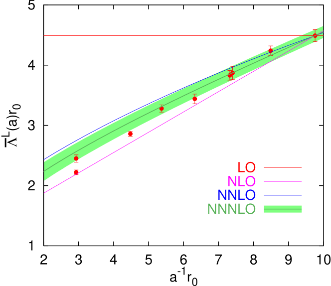
Figure 15: Perturbative running of the binding energy $\overline{\Lambda}$ in the lattice scheme, in comparison with lattice data, starting at the smallest available lattice spacing. The NNNLO error band incorporates the error due to the uncertainty in $\Lambda_{\overline{\rm MS}}$ [37], and the statistical error.

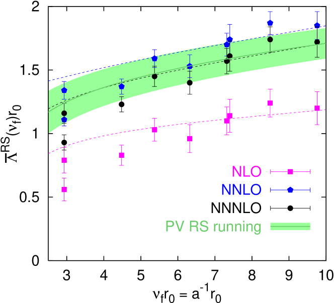
Figure 16: The binding energy $\overline{\Lambda}$, obtained on the lattice and converted into the RS scheme at NLO (squares), NNLO (pentagons), NNNLO (circles) and the result of Eq. (81), run to different scales using the PV prescription (neglecting the “theoretical” errors). The dashed lines are explained in the text.

$\overline{\Lambda}^{L}(a)$ has been calculated on a variety of lattice spacings by different collaborations [48, 34, 49, 50]. The main source of uncertainty in these determinations is the extrapolation to zero light quark mass. We used the $r_{0}/a$ values from the interpolation of Ref. [51] to assign the scale. The results are displayed in Table 5 and are roughly consistent with each other, with the exception of the coarsest lattice point $r_{0}\approx 2.93\,a$ that corresponds to $\beta=5.7$. Here the raw data of Ref. [50] are more accurate but the chiral extrapolation of Ref. [34] should be better controlled.

We multiply the values obtained for $\Lambda_{B}^{L}r_{0}$ of Ref. [12] (that are displayed in Table 3) by the colour factor $C_{f}/C_{A}$. At $\beta=5.7,6.0$ and 6.2, respectively, we obtain the numerical values $2.37(4)$, $3.11(2)$ and $3.72(2)$. The corresponding values in Table 5 read $2.45(6)|2.22(4)$, $3.28(6)$ and $3.83(8)|3.87(11)$ where for both, $\beta=5.7$ and $\beta=6.2$, two independent determinations exist. The qualitative agreement is remarkable: not only the perturbative expansions of $\delta\Lambda$ and $\delta m_{\rm stat}$ are dominated by terms that are proportional to the respective Casimirs of the gauge group representation of the static source but also the non-perturbative values themselves. In fact also in the $\rm RS$ scheme the result Eq. (66) is close to the value displayed in Eq. (76), multiplied by $C_{A}/C_{f}=9/4$.

Similar to the discussion in Sec. 5.2 above, we can translate the results from the lattice scheme into the $\rm RS$ scheme. The master formula in this case is very similar to Eq. (69) and reads (known to NNNLO),

$$\overline{\Lambda}^{\rm RS}(\nu_{f})=\overline{\Lambda}^{L}(a)-\left[\delta m_{\rm stat}^{L}(a)-\delta m_{\rm RS}(\nu_{f})\right]\,,$$ (77)

with

$$\delta m_{\rm stat}^{L}(a)-\delta m_{\rm RS}(\nu_{f}) = \frac{C_{f}}{2}v_{1}a^{-1}\alpha_{\rm s}(\nu)$$

$$+ \left\{\frac{C_{f}}{2}\frac{a^{-1}}{4\pi}\left[v_{2}+v_{1}B_{1}(\nu a)\right]+\frac{\nu_{f}}{2}{\tilde{V}}_{s,1}\right\}\alpha_{\rm s}^{2}(\nu)$$

$$+ \left\{\frac{C_{f}}{2}\frac{a^{-1}}{(4\pi)^{2}}\left\{v_{3}+2v_{2}B_{1}(\nu a)+v_{1}\left[B_{2}(\nu a)+B_{1}^{2}(\nu a)+b_{1}^{2}\right]\right\}\right.$$

$$\left.\quad+\frac{\nu_{f}}{2}\left[{\tilde{V}}_{s,2}-\tilde{V}_{s,1}\frac{\beta_{0}}{\pi}\ln\left(\frac{\nu_{f}}{\nu}\right)\right]\right\}\alpha_{\rm s}^{3}(\nu)+\cdots\,,$$

where,

$$B_{i}(x)=-b_{i}+2\beta_{i-1}\ln(x),\quad i=1,2\,,$$ (79)

and the coefficients $\tilde{V}_{s,1}$ and $\tilde{V}_{s,2}$ can be found in Table 2. The coefficients $v_{i}$ and $b_{i}$ can be found in Eqs. (38) – (40) and Eqs. (42) and (43), respectively.

Eqs. (77) and (6.1) also relate results obtained at different lattice spacings to each other,

$$\overline{\Lambda}^{L}(a^{\prime})=\overline{\Lambda}^{L}(a)-\left[\delta m^{L}_{\rm stat}(a)-\delta m^{L}_{\rm stat}(a^{\prime})\right]\,.$$ (80)

To illustrate this we display the $\Lambda^{L}(a)$ values of Table 5 in Fig. 15, together with the expected running, starting at the finest, i.e. right-most, lattice point at LO, NLO, NNLO and NNNLO. The NNNLO error band contains both, the statistical error and that due to the uncertainty in $\alpha_{s}(a)$. The running is done in each order in a self-consistent way to the given order in $\alpha_{\rm s}$, according to Eq. (6.1) (without the $\tilde{V}_{s,i}$ terms). We used $\nu=9.76\,r_{0}^{-1}$ and the initial value, $\alpha_{\rm s}(\nu)$, was calculated from $\Lambda_{\overline{\rm MS}}r_{0}$ using the four loop running. We observe convergence and moreover the series is sign alternating. To NNNLO, except for the lower lying of the two $r_{0}/a\approx 2.93$ data points, there is no contradiction between data and the expectation. However, the points of Ref. [34] have a slightly more pronounced slope such that the $r_{0}/a\approx 2.9,4.5$ and 6.3 points ($\beta=5.7,5.9$ and 6.1) lie below the curve while the $r_{0}/a\approx 8.5$ point ($\beta=6.3$) lies somewhat above.

We also display the data of the table in Fig. 16, in analogy to Fig. 14 but disregard the LO result that is already displayed in Fig. 15. The size of $\delta m^{L}_{\rm stat}(a)-\delta m_{\rm RS}(a^{-1})$ increases linearly in $a^{-1}$, with logarithmic corrections: at coarse lattice spacings there might be significant perturbative $O(\alpha_{s}^{4})$ and non-perturbative $O(a^{2}/r_{0}^{2})$ corrections affecting the slope of this function while at fine lattice spacings the slope can be determined accurately but the $\delta m$-difference itself becomes large. An accurate conversion between the two schemes can therefore neither be obtained at extremely fine nor at very coarse lattice spacings. Setting $\nu=\nu_{f}$, the difference between NLO and NNLO translation is minimised for $3{\ \lower-1.2pt\vbox{\hbox{\hbox to0.0pt{$<$\hss}\lower 6.0pt\vbox{\hbox{$\sim$}}}}\ }r_{0}\nu_{f}{\ \lower-1.2pt\vbox{\hbox{\hbox to0.0pt{$<$\hss}\lower 6.0pt\vbox{\hbox{$\sim$}}}}\ }4$ while that between NNLO and NNNLO is minimal for $7.5{\ \lower-1.2pt\vbox{\hbox{\hbox to0.0pt{$<$\hss}\lower 6.0pt\vbox{\hbox{$\sim$}}}}\ }r_{0}\nu_{f}{\ \lower-1.2pt\vbox{\hbox{\hbox to0.0pt{$<$\hss}\lower 6.0pt\vbox{\hbox{$\sim$}}}}\ }9$, where the widths of these bands are determined by our uncertainty in the value of $\Lambda_{\overline{\rm MS}}r_{0}$.

We choose to translate the lattice scheme results into the $\rm RS$ scheme by means of a global NNNLO fit to the $r_{0}/a>5$, i.e. $\beta\geq 6.0$ data, expanded in terms of $\alpha_{s}(\nu=9.76\,r_{0}^{-1})$, where we set $\nu_{f}=\nu$. The result reads,

$$\overline{\Lambda}^{\rm RS}(\nu_{f}=9.76\,r_{0}^{-1})=\left[1.70\pm 0.08({\rm latt.})\pm 0.18({\rm th.})\pm 0.04(\Lambda_{\overline{\rm MS}})\right]\,r_{0}^{-1}\,.$$ (81)

Note that $\overline{\Lambda}^{\rm RS}$ is the only fit parameter.

The dashed curves in Fig. 16 correspond to such an NNNLO fit to the LO results, subsequently transformed in the same way as the data points to NLO, NNLO and NNNLO. The error band corresponds to the result Eq. (81) above, without the theoretical error, run to different energies, using the PV prescription, Eq. (61): unlike the band displayed in Fig. 14 above, this is not the result of an independent determination. We would also have found agreement with the result Eq. (76), but only within the large theoretical errors of this un-quenched determination.

At high order in the perturbative expansion and at high energies one would expect the slope of the non-perturbative running in the lattice scheme, translated into the RS scheme, to approach that of the running within the RS scheme. Discarding the four data points of Ref. [34], Fig. 16 nicely confirms this expectation. We will investigate this running with higher accuracy in Sec. 6.3 below.

The errors of the determination Eq. (81) above stem from the following sources:

1) “latt.” is the sum of the statistical error ($\pm 0.03$) and the error encountered when varying the fit range $a^{-1}_{\min}r_{0}=4.48,5.37,6.32$ ($\pm 0.05$): $\pm 0.08$.

2) “th.” is the sum of perturbative and non-perturbative errors. As perturbative error we take the difference between NNLO and NNNLO results. Varying the fit range as above this difference never exceeds $\pm 0.04$. We also study the error due to the uncertainty of $N_{V_{s}}$ obtaining $\pm 0.06$. To investigate possible non-perturbative effects we include an $a^{2}$ term into the fit. We estimate an additional $\pm 0.08$ uncertainty. Adding these three errors linearly results in $\pm 0.18$.

3) “$\Lambda_{\overline{\rm MS}}$” stands for the uncertainty in the determination of $\Lambda_{\overline{\rm MS}}r_{0}$ [37]: $\pm 0.04$.

Using the running in the RS scheme (we note that the error due to the uncertainty of $N_{V_{s}}$ almost cancels in the running) we obtain,

$$\overline{\Lambda}^{\rm RS}(\nu_{f}=2.5\,r_{0})=\left[1.17\pm 0.08({\rm latt.})\pm 0.13({\rm th.})\pm 0.09(\Lambda_{\overline{\rm MS}})\right]\,r_{0}^{-1}\,.\,$$ (82)

from the value Eq. (81). This $n_{f}=0$ result compares reasonably well with the phenomenological $n_{f}=4$ value of Eq. (76) above and its error is of a comparable size.

6.2 Comment on the $b$ quark mass

We cannot resist the temptation to obtain a value for the $\rm RS$ scheme bottom quark mass, using Eq. (74) and our quenched result Eq. (82). We obtain,

$$m_{b,\rm RS}(\nu_{f}=1\,{\rm GeV})=\left[4849\pm 32({\rm latt.})\pm 60({\rm th.})\pm 35(\Lambda_{\overline{\rm MS}})\right]\,{\rm MeV}\,,\,$$ (83)

where we have translated Eq. (82) into physical units for $\nu_{f}=1$ GeV and also added an extra theoretical error of $\pm 30$ MeV, due to $1/m_{b}$ corrections, combined quadratically with the theoretical error inherited from the lattice determination of $\overline{\Lambda}^{\rm RS}$. From this number we can compute the $\overline{\rm MS}$ scheme result,

$$m_{b,\overline{\rm MS}}(m_{b,\overline{\rm MS}})=\left[4191\pm 29({\rm latt.})\pm 47({\rm th.})\pm 1(\Lambda_{\overline{\rm MS}})\right]\,{\rm MeV}\,,$$ (84)

where we have performed any running and manipulation with $n_{f}=4$ and used the PV prescription to run $m_{b,\rm RS}$ from 1 GeV up to the bottom $\overline{\rm MS}$ mass. In this way higher order terms in the relation between the $\overline{\rm MS}$ and the RS mass are minimized. If instead one determines $m_{b,\overline{\rm MS}}(m_{b,\overline{\rm MS}})$ directly from its perturbative relation with $m_{b,\rm RS}(1\,\mbox{GeV})$ one obtains a somewhat larger result, but with sizeable higher order terms. Note that some of the theoretical errors, such as the uncertainty of $N_{V_{s}}$, are correlated with the running of $\alpha_{\rm s}$.

Obviously one has to allow for quenching errors. Naïvely one might assume an $O(10~{}\%)$ effect on the binding energy which amounts to 50 MeV in Eq. (83). However, this might be an underestimate since the running of the mass with the scale in the $n_{f}=0$ case is very different from that for $n_{f}=4$ and the relative effect on $\overline{\Lambda}\ll m_{b}$, due to a different running, is larger than that on the quark mass. To illustrate this we also work consistently with $n_{f}=0$ and obtain,

$$m_{b,\overline{\rm MS}}(m_{b,\overline{\rm MS}})=\left[4339\pm 29({\rm latt.})\pm 49({\rm th.})\pm 9(\Lambda_{\overline{\rm MS}})\right]\,{\rm MeV}\,:$$ (85)

this differs from the value Eq. (84) by almost 150 MeV. Note that we have used the $n_{f}=0$ value $\Lambda_{\overline{\rm MS}}=0.602\,r_{0}^{-1}$ to obtain the above results. Using the $n_{f}=5$ QCD world average $\alpha_{s}(M_{z})=0.118$ instead (running it across the bottom flavour threshold down to 1 GeV), the central value of Eq. (84) would read, $m_{b,\overline{\rm MS}}(m_{b,\overline{\rm MS}})=4113$ MeV. The difference between these two values may also be indicative of the typical size of the error due to quenching.

We feel that 1 GeV might be a more natural scale to obtain an $n_{f}=4$ prediction from the quenched model than 4 GeV and hence prefer the central value of Eq. (84). After all, the quenched model has been adjusted to reproduce low energy QCD phenomenology and indeed Eqs. (76) and (82) agree with each other within errors. However, as discussed above and as indicated by the 150 MeV difference from using a different perturbative running, such predictions have to be consumed with some caution. Eq. (84) demonstrates the precision that can be achieved in lattice simulations of static-light mesons with sea quarks to NNNLO. Obviously, the “latt.” error can systematically be reduced. Note that, with NNNLO perturbative results, the dominant theoretical uncertainty (apart from the sea quark content) is due to $1/m_{b}$ corrections.

6.3 The running of $\overline{\Lambda}$ from the static lattice potential

To leading order, the singlet static energy $E_{s}$ is the sum of twice the heavy quark mass and the singlet potential, Eq. (2), while $M_{B}$ is the sum of the quark mass and the binding energy $\overline{\Lambda}$, Eq. (7). Consequently, in the $\rm OS$ ($\rm RS$) schemes $V_{s}$ contains twice the leading renormalon (power term) of $\overline{\Lambda}$. In QCD with sea quarks this is also evident from the large distance behaviour, where $E_{s}(r)$ will approach $2M_{B}$.

In the lattice scheme, the non-perturbative energy $E^{L}_{\Sigma_{g}^{+}}$ differs from $E_{s}$ by twice the quark mass, Eq. (45), and contains the same power term as the static-light energy $\overline{\Lambda}^{L}$ (times two). One can explicitly verify this in perturbation theory. In QCD with sea quarks $E^{L}_{\Sigma_{g}^{+}}(r)$ will approach $2\overline{\Lambda}^{L}$ for $r{\ \lower-1.2pt\vbox{\hbox{\hbox to0.0pt{$>$\hss}\lower 6.0pt\vbox{\hbox{$\sim$}}}}\ }r_{c}$, where $r_{c}$ denotes the distance associated with “string breaking” and is implicitly defined by, $E_{s}(r_{c})=2M_{B}$. We find the static potential [52, 46] $E_{\Sigma_{g}^{+}}$ to exceed the values of $2\overline{\Lambda}^{L}$ of Ref. [48] at $r>r_{c}=(2.25\pm 0.15)\,r_{0}$, a distance that is statistically indistinguishable from the value $r_{c}\approx 2.3\,r_{0}$, obtained in simulations with $n_{f}=2$ light sea quarks [3, 13].

$a^{-1}r_{0}$	$\overline{\Lambda}^{L}_{\rm pot}r_{0}$	$\overline{\Lambda}^{\rm RS}r_{0}$(NLO)	$\overline{\Lambda}^{\rm RS}r_{0}$(NNLO)	$\overline{\Lambda}^{\rm RS}r_{0}$(NNNLO)
1.95	2.11(10)	0.64(14)	1.30(10)	0.99(12)
2.42	2.35(10)	0.81(12)	1.39(10)	1.16(11)
2.94	2.51 (4)	0.86 (8)	1.40 (5)	1.22 (6)
3.80	2.81 (5)	0.95 (8)	1.49 (5)	1.33 (6)
4.47	3.02 (3)	1.00 (7)	1.54 (4)	1.39 (5)
5.35	3.29 (2)	1.05 (7)	1.61 (4)	1.46 (5)
7.30	3.84 (2)	1.13 (7)	1.73 (4)	1.59 (5)
9.89	4.53 (2)	1.21 (8)	1.87 (5)	1.73 (6)
12.74	5.23 (3)	1.26 (9)	1.99 (6)	1.85 (7)
14.36	5.47(10)	1.16(13)	1.92(12)	1.78(12)

Table 6: The inverse lattice spacing, the estimate of the static-light binding energy in the lattice scheme, $\overline{\Lambda}^{L}_{\rm pot}=E_{\Sigma_{g}^{+}}^{L}(r_{0})/2+\Delta$, Eqs. (86) and (87), as well as its conversion to the RS scheme to different orders in perturbation theory. The errors only incorporate the statistical uncertainties of the $E_{\Sigma_{g}^{+}}(r_{0})$ data, as well as the 8 % uncertainty in $\Lambda_{\overline{MS}}r_{0}$ [37], added in quadrature. The overall error due to the uncertainty in $\Delta$, which does not affect the running of $\overline{\Lambda}^{L}$, is not displayed.

The difference $2\overline{\Lambda}^{L}-E_{\Sigma_{g}^{+}}^{L}(r_{0})=E_{\Sigma_{g}^{+}}^{L}(r_{c})-E_{\Sigma_{g}^{+}}^{L}(r_{0})$ is a constant, up to $O(a^{2})$ lattice artifacts. In what follows we will investigate the running of,

$$\overline{\Lambda}^{L}_{\rm pot}(a)=\frac{1}{2}E_{\Sigma_{g}^{+}}^{L}(r_{0};a)+\Delta,$$ (86)

as a function of $a^{-1}$. The static lattice potential $E_{\Sigma_{g}^{+}}(r_{0})/2$ can be determined more precisely than $\overline{\Lambda}^{L}$: in terms of computer time it is cheaper to obtain with the same statistical error and, since no chiral extrapolation is involved, with virtually no systematic uncertainties. However, we do not know the absolute normalization $\Delta$. We re-analyse the lattice potentials of Refs. [52, 46], to correctly account for the propagation of the uncertainty of $r_{0}$ into the combination $r_{0}E_{\Sigma_{g}^{+}}(r_{0})$. By matching the lattice potential $E_{\Sigma_{g}^{+}}^{L}(r_{0})/2=(2.856\pm 0.014)\,r_{0}^{-1}$ to $\overline{\Lambda}^{L}=(3.844\pm 0.065)\,r_{0}^{-1}$ at $\beta=6.2$ ($r_{0}/a\approx 7.3$), where we have two independent results for the latter quantity [48, 49], we obtain

$$\Delta=(0.988\pm 0.067)\,r_{0}^{-1}\,.$$ (87)

For ease of comparison with Sec. 6.1, we display the resulting $\overline{\Lambda}^{L}_{\rm pot}(a)$ in Table 6 as well as in the figures. The additional uncertainty due to the error in $\Delta$ should be kept in mind.

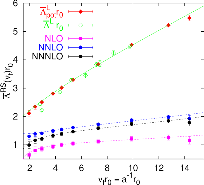
Figure 17: The binding energy $\overline{\Lambda}^{L}_{\rm pot}$, Eq. (86), in the lattice scheme (full diamonds), in comparison with $\overline{\Lambda}^{L}$ of Sec. 6.1 (open diamonds). The constant $\Delta$ has been adjusted by requiring agreement between the two data sets at $r_{0}\approx 7.3\,a$. The uncertainty of $\Delta=(0.988\pm 0.067)\,r_{0}^{-1}$ is not included into the errors. NLO, NNLO and NNNLO refer to transformations of $\overline{\Lambda}^{L}_{\rm pot}$ into the RS scheme to different orders in perturbation theory. The solid line corresponds to the NNNLO expectation with $\Lambda_{\overline{\rm MS}}\approx 0.602\,r_{0}^{-1}$, and the central value of Eq. (81), $\overline{\Lambda}^{\rm RS}(\nu_{f}=9.76\,r_{0}^{-1})=1.70\,r_{0}^{-1}$.

We display $\overline{\Lambda}^{L}_{\rm pot}$ in Table 6, together with conversions into the RS scheme, according to Eqs. (77) and (6.1). The data are also depicted in Fig. 17 (full diamonds), together with the results from the static-light energies $\overline{\Lambda}^{L}$ (open diamonds). Except for the four data points of Ref. [34] at $r_{0}/a\approx 2.9,4.5,6.3$ and 8.5, whose slope is somewhat incompatible with the results from the other references as well as with perturbation theory (as we already noticed in Sec. 6.1 above), we find agreement between the non-perturbative running of $E_{\Sigma_{g}^{+}}(r_{0})/2$ and that of $\overline{\Lambda}^{L}$, down to the lowest scales. This need not be so since in principle the results may differ by $O(a^{2}/r_{0}^{2})$ lattice terms. We also compare this running with the expectation from the value $\Lambda_{\overline{\rm MS}}\approx 0.602\,r_{0}^{-1}$ (solid line), where we use the normalization suggested by the central value of Eq. (81), $\overline{\Lambda}^{\rm RS}(\nu_{f}=9.76\,r_{0}^{-1})\approx 1.70\,r_{0}^{-1}$.

As can be seen there is no contradiction between the lattice data and NNNLO perturbation theory down to scales as low as $2\,r_{0}^{-1}$ and as high as $15\,r_{0}^{-1}$. This agreement is quantifiable: a one-parameter NNNLO fit to the $a^{-1}>5\,r_{0}^{-1}$ data (setting $\Lambda_{\overline{\rm MS}}=0.602\,r_{0}^{-1}$) yields $\chi^{2}/N_{DF}=3.53/4$, with the value (translated into the RS scheme for ease of comparison),

$$\overline{\Lambda}^{\rm RS}(9.76\,r_{0}^{-1})=(1.71\pm 0.01)\,r_{0}^{-1}\,.$$ (88)

Including all available data results in $\chi^{2}/N_{DF}=6.91/9$ with $\overline{\Lambda}^{\rm RS}(9.76\,r_{0}^{-1})=(1.70\pm 0.01)\,r_{0}^{-1}$. The errors of the above examples are purely statistical. The uncertainties in $\Delta$ and $\Lambda_{\overline{\rm MS}}$ as well as theoretical errors are unaccounted for. If we go to NNLO we obtain the $\chi^{2}/N_{DF}$ values of 16.3 (all data points), 23.0 ($a^{-1}>5\,r_{0}^{-1}$) and 6.7 ($a^{-1}>9\,r_{0}^{-1}$). Also, the predicted value of $\overline{\Lambda}^{\rm RS}(9.76\,r_{0}^{-1})r_{0}$ becomes somewhat unstable, ranging from 1.76 (all data points), 1.79 ($a^{-1}>5\,r_{0}^{-1}$), up to 1.91 ($a^{-1}>9\,r_{0}^{-1}$): within the accuracy of the data it is essential to go to at least NNNLO in perturbation theory.

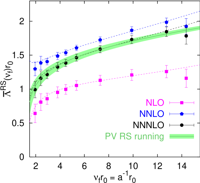
Figure 18: The binding energy $\overline{\Lambda}^{L}_{\rm pot}$, Eq. (86), translated into the RS scheme at NLO (squares), NNLO (pentagons) and NNNLO (circles). We have neglected an overall error in the vertical scale of $\pm 0.067\,r_{0}^{-1}$, due to the uncertainty of $\Delta$, that does not affect the running. The dashed lines correspond to the NNNLO running in the lattice scheme with $\Lambda_{\overline{\rm MS}}=0.602\,r_{0}^{-1}$, where we used the fit result Eq. (88), $\overline{\Lambda}^{\rm RS}(9.76\,r_{0}^{-1})\approx 1.71\,r_{0}^{-1}$, as normalization. The error band corresponds to the prediction Eq. (81), $\overline{\Lambda}^{\rm RS}(9.76\,r_{0}^{-1})=(1.70\pm 0.04)\,r_{0}^{-1}$, and includes the uncertainty due to $\Lambda_{\overline{\rm MS}}=(0.602\pm 0.048)\,r_{0}^{-1}$ (but no other errors).

In Fig. 17 and Table 6 we have also displayed the results, translated into the RS scheme to different orders in perturbation theory. In Fig. 18 we focus on this comparison. This figure very much resembles Fig. 16, only that now the error bars are smaller as we discard the error of $\Delta$, which will only affect the overall value of $\overline{\Lambda}$ but not the running with the scale. The dashed lines correspond to NNNLO perturbation theory in the lattice scheme with $\Lambda_{\overline{\rm MS}}=0.602\,r_{0}^{-1}$, and the central value of Eq. (88) as normalization point. This running perfectly agrees with the data down to very low energies. As already observed in Sec. 6.1 above, we also find nice convergence for $a^{-1}{\ \lower-1.2pt\vbox{\hbox{\hbox to0.0pt{$>$\hss}\lower 6.0pt\vbox{\hbox{$\sim$}}}}\ }3\,r_{0}^{-1}$, as the order of the perturbation theory is increased. The error band corresponds to the PV prescription of the running in the RS scheme with $\overline{\Lambda}^{\rm RS}(9.76\,r_{0}^{-1})=(1.70\pm 0.04)\,r_{0}^{-1}$, run to different scales, using $\Lambda_{\overline{\rm MS}}=(0.602\pm 0.048)\,r_{0}^{-1}$. Note that the errors that we display in this case are only due to the uncertainty in $\alpha_{\rm s}$, with all other error sources of Eq. (81) (as well as the uncertainty of $\Delta$) ignored.

We find excellent agreement between data and the predicted running. In fact, one can in principle determine $\alpha_{\rm s}$ from the logarithmic corrections to the $a^{-1}$ running of the binding energy: in dedicated lattice simulations of the short distance static potential tremendous statistical accuracy can be achieved and tiny lattice spacings are accessible [25]. Even using our static singlet potentials [52, 46] that are less accurate than those of this recent reference, a two-parameter NNNLO fit to the $a^{-1}>5\,r_{0}^{-1}$ data yields, $\Lambda_{\overline{\rm MS}}=(0.590\pm 0.036)\,r_{0}^{-1}$ and $\overline{\Lambda}^{\rm RS}(9.76\,r_{0}^{-1})=(1.73\pm 0.04)\,r_{0}^{-1}$ with $\chi^{2}/N_{DF}=3.35/3$. Including the whole energy range, down to $a^{-1}\approx 2\,r_{0}^{-1}$, results in, $\Lambda_{\overline{\rm MS}}=(0.627\pm 0.026)\,r_{0}^{-1}$ and $\overline{\Lambda}^{\rm RS}(9.76\,r_{0}^{-1})=(1.68\pm 0.02)\,r_{0}^{-1}$, still with very acceptable $\chi^{2}/N_{DF}=6.08/8$. The results for $\overline{\Lambda}^{\rm RS}$ are in perfect agreement with those obtained in Eqs. (81) and (88) above. Moreover, the fits are consistent with the value of Ref. [37], $\Lambda_{\overline{\rm MS}}=(0.602\pm 0.048)\,r_{0}^{-1}$, within statistical errors smaller than the uncertainty of this reference value.

In conclusion, we have demonstrated that the running of the binding energy in the lattice scheme can be reproduced with incredible accuracy in NNNLO perturbation theory, in terms of $\alpha_{\rm s}$. This accuracy is possible since, unlike in the case of the binding energy itself, there is no leading renormalon contribution to its running. Down to energies of about 1 GeV we do not see any sign of a break-down of perturbation theory or evidence of significant non-perturbative contributions to the running. We have also confirmed that the theoretical errors estimated in Eqs. (81) and (82) are indeed conservative.

7 Gluinonium and other related issues

We already mentioned that gluelumps are interesting in the context of bound states including heavy adjoint particles, such as gluinos of SUSY models (even if it is quite likely that they will decay before any kind of hadronization takes place). In this case, to leading order in HGET (Heavy Gluino Effective Theory), the gluino mass can be obtained from the relation,

$$M_{\tilde{G}}=\Lambda_{B}^{\rm OS}+m_{\tilde{g},\rm OS}=\Lambda_{B}^{\rm RS}(\nu)+m_{\tilde{g},\rm RS}(\nu),$$ (89)

in a scheme of choice that can then be converted into the mass in say the $\overline{\rm MS}$ scheme $\overline{m}_{\tilde{g}}(\overline{m}_{\tilde{g}})$, analogously to the discussion of Sec. 6 above. We will limit most of the discussion below to the $\rm RS$ and $\rm OS$ schemes but translation into lattice schemes is straight forward.

$M_{\tilde{G}}$ denotes the mass of the lightest (spin-averaged) glueballino. Note that in this context the gluelump energy $\Lambda_{B}$ plays the same rôle as the binding energy $\overline{\Lambda}$ did for heavy-light mesons. We have $\Lambda_{H}^{\rm RS}(\nu_{f})=\Lambda_{H}^{\rm OS}-\delta\Lambda_{\rm RS}(\nu_{f})$ and hence,

$$m_{\tilde{g},\rm RS}(\nu_{f})=m_{\tilde{g},\rm OS}+\delta\Lambda_{\rm RS}(\nu_{f})\,:$$ (90)

$\delta m_{\tilde{g},\rm RS}=-\delta\Lambda_{\rm RS}$ in the glueballino case corresponds to the $\delta m_{\rm RS}$ of heavy-light mesons. We can also write down the above equations in the lattice scheme in which case, using the same conventions as in other parts of this paper, $\delta m_{\tilde{g},L}=\delta\Lambda_{L}$.

In addition to glueballinos one can imagine gluino-gluino bound states: gluinonia, $\Gamma$. Their dynamics is dictated by the following Lagrangian,

$$L_{\rm pNRQCD,\Gamma}=\int d^{3}{\bf r}\,d^{3}{\bf R}\,{\rm Tr}\,\Biggl{\{}{\rm S_{\Gamma}}^{\dagger}\left(i\partial_{0}-V_{A,s}\right){\rm S_{\Gamma}}+{\rm O_{\Gamma,1}}^{\dagger}\left(iD_{0}-V_{A,o}\right){\rm O_{\Gamma,1}}+\cdots\Biggr{\}}\,,$$ (91)

at leading order in $1/m_{\tilde{g}}$ and in the multipole expansion. This is analogous to Eq. (1), replacing the static sources in the fundamental by static sources in the adjoint representation. This means that there will be further multiplets in Eq. (91) that we will not consider in this paper.

The singlet potential between two adjoint sources $V_{A,s}(r)$ has been calculated in perturbation theory to $O(\alpha_{\rm s}^{2})$ and the corresponding energy $E_{A}^{L}(r;a)$ was determined in lattice simulations (see e.g. Ref. [24]). Up to lattice artifacts $\propto a^{2}$ we can write,

$$E_{A}(r) = 2m_{\tilde{g},L}(a)+E_{A}^{L}(r;a)$$ (92)

$$= 2m_{\tilde{g},L}(a)+V_{A,s,L}(r;a)+O(r^{2})$$ (93)

$$= 2m_{\tilde{g},\rm RS}(\nu_{f})+V_{A,s,\rm RS}(r;\nu_{f})+O(r^{2}),$$ (94)

where the normalization of $E_{A}^{L}(r)$ with respect to $E_{A}(r)$ can be obtained from the gluinonium spectrum. Obviously,

$$\lim_{r\rightarrow\infty}E_{A}(r)=2M_{\tilde{G}},$$ (95)

while for the bottomonium energy in QCD with sea quarks one obtains (up to $1/m_{b}$ corrections and neglecting radial and gluonic excitations),

$$\lim_{r\rightarrow\infty}E_{s}(r)=\lim_{r\rightarrow\infty}E_{H}(r)=2M_{B}.$$ (96)

In combining Eq. (94) with Eqs. (26) and (30) we obtain the important equality,

$$E_{A}(r)+2[E_{B}(r)-E_{s}(r)]=V_{A,s,\rm RS}(r;\nu_{f})+2[V_{o,\rm RS}(r;\nu_{f})-V_{s,\rm RS}(r;\nu_{f})]+2M_{\tilde{G}}+O(r^{2})\,,$$ (97)

where we have used the fact that $M_{\tilde{G}}=m_{\tilde{g},\rm RS}+\Lambda_{B}^{\rm RS}$ and $E_{B}\in\{E_{\Pi_{u}},E_{\Sigma_{u}^{-}}\}$. The effect of $\delta m_{\rm RS}$ cancels from the combination $E_{B}-E_{s}$ and $\delta\Lambda_{\rm RS}$ from $E_{A}+2E_{H}$. Since the glueballino mass is a physical observable this implies that, up to $O(r^{2})$ corrections, the combination $V_{A,s}(r)+2[V_{o}(r)-V_{s}(r)]$ is scale independent and free of renormalon and power contributions: the UV renormalon of $V_{o}$ is cancelled by the UV renormalon of $V_{s}$ while the leading IR renormalon of $V_{o}$, which we studied in this paper, is cancelled by one half of the UV renormalon of $V_{A,s}$. In fact, to $O(\alpha_{\rm s}^{2})$ this combination explicitly vanishes and the $O(\alpha_{\rm s}^{3})$ term is suppressed by a colour factor $1/N_{c}^{2}$.

In the above equation $E_{B}(r)$ corresponds to the $\Pi_{u}$ or $\Sigma_{u}^{-}$ hybrid levels. For a general $E_{H}(r)$ we would have to replace the $M_{\tilde{G}}$ on the rhs by the mass of the excited glueballino in the respective channel. At $r\rightarrow\infty$ the rhs of Eq. (97) will approach $2M_{\tilde{G}}$, see Eqs. (95) and (96).

We wish to compare our expectation with lattice data. This can either be done after an extrapolation of these to the continuum limit or at finite lattice spacing in the lattice scheme. Re-expressing Eq. (97) in terms of the energy levels as determined in the lattice scheme [$E_{A}(r)=E_{A}^{L}(r;a)+2m_{\tilde{g},L}(a)$ etc.], and using the conventions of Sec. 4.4 above, this amounts to,

$$E_{A}^{L}(r;a)+2[E_{\Pi_{u}}^{L}(r;a)-E_{\Sigma_{g}^{+}}^{L}(r;a)-\Lambda_{B}^{L}(a)]$$ (98)

$$\qquad\qquad=V_{A,s,L}(r;a)+2[V_{o,L}(r;a)-\delta\Lambda_{L}(a)-V_{s,L}(r;a)]+O(r^{2})+\cdots$$

$$\qquad\qquad=O(r^{2})+O(\alpha_{\rm s}^{3}/N_{c}^{2})+O(\Lambda_{\rm QCD}^{2}a^{2})+O(a^{2}/r^{2})\,.$$

Both lhs and rhs of the above equation are explicitly free of $a^{-1}$ power terms (and of leading renormalons). In fact the rhs vanishes in perturbation theory, to at least $O(\alpha_{\rm s}^{3}/N_{c}^{2})$. As indicated in the equation, in general there will be non-perturbative $O(a^{2}/r^{2})$ as well as $O(\Lambda_{\rm QCD}^{2}a^{2})$ lattice artifacts, in addition to the $O(r^{2})$ corrections from higher terms in the multipole expansion.

The above combination is extremely interesting as for small $r$ there should only be a quadratic but no linear term. At $r{\ \lower-1.2pt\vbox{\hbox{\hbox to0.0pt{$>$\hss}\lower 6.0pt\vbox{\hbox{$\sim$}}}}\ }2\,r_{0}$ the adjoint string will break and the lhs of the equation will approach zero like $1/r$. In the intermediate region $0.5\,r_{0}<r<2\,r_{0}$ one would expect two non-perturbative contributions, a linear term from the slope of $E_{A}(r)$, with an effective string tension [24], $\sigma_{\rm eff}=[3.09\pm 0.10]r_{0}^{-2}$, as well as a $1/r$ term that dominantly originates from the difference between static hybrid and singlet potentials and whose coefficient will approach $2\pi$ as $r\rightarrow\infty$, in an effective string model expectation. In fact for $r\approx r_{0}$ one would expect this $1/r$ term still to dominate over the linear term.

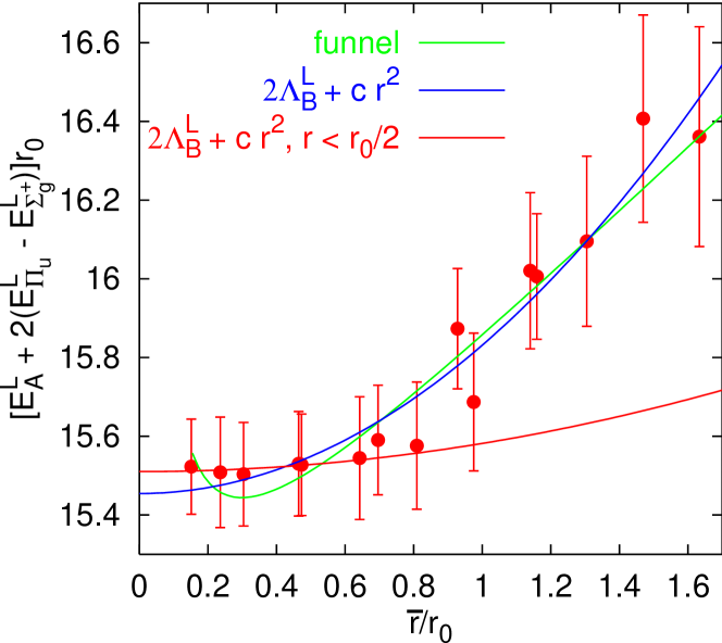
Figure 19: The combination $E^{L}_{A}(r)+2[E^{L}_{\Pi_{u}}(r)-E^{L}_{\Sigma_{g}^{+}}(r)]$, Eq. (98), as a function of $\overline{r}=r[1+O(a^{2}/r^{2})]$, Eq. (10), together with various fits, on an anisotropic lattice with resolution $a_{\sigma}\approx 4\,a_{\tau}\approx 0.16\,r_{0}$.

We wish to compare this expectation to numerical data. Unfortunately, on isotropic lattices where we know the gluelump mass in the lattice scheme we did not compute the adjoint potential while on our anisotropic data sets all potentials, singlet, adjoint and hybrid are available but the gluelump mass is unknown. In Fig. 19 we display the combination $E^{L}_{A}(r)+2[E^{L}_{\Pi_{u}}(r)-E^{L}_{\Sigma_{g}^{+}}(r)]$ as a function of $\overline{r}=r[1+O(a^{2}/r^{2})]$, Eq. (10), at our finest anisotropic lattice spacing, $a_{\sigma}\approx 0.16\,r_{0}\approx 4\,a_{\tau}$ which, within errors, is compatible with the continuum limit, see Sec. 3 and Ref. [24]. Note that there is an additional 1 % overall error on ordinate and abscissa due to the conversion from lattice units into units of $r_{0}$ that we do not display.

From Eq. (98) we would expect the combination shown to approach the gluelump energy in the lattice scheme, $\Lambda_{B}^{L}(a)$, as $r\rightarrow 0$. We see that the approach towards this limit is remarkably flat. In fact, excluding the $r>0.9\,r_{0}$ data, which are clearly in the non-perturbative regime anyway, we are unable to resolve deviations of the data from a constant. Note that the units on the ordinate, $0.2\,r_{0}^{-1}\approx 80$ MeV, are quite small. A linear plus quadratic fit,

$$E_{A}^{L}(r)+2[E_{\Pi_{u}}^{L}(r)-E_{\Sigma_{g}^{+}}(r)]=2\Lambda_{B}^{L}+c\,r^{2}\,,$$ (99)

to $r<0.5\,r_{0}$ data yields,

$$2\Lambda_{B}^{L}=(15.51\pm 0.10)\,r_{0}^{-1},\qquad c=(0.07\pm 0.70)\,r_{0}^{-3}\,.$$ (100)

A purely phenomenological fit to the same functional form for all distances results in,

$$2\Lambda_{B}^{L}=(15.45\pm 0.06)\,r_{0}^{-1},\qquad c=(0.38\pm 0.07)\,r_{0}^{-3}\,,$$ (101)

while in a physically completely unmotivated funnel parametrisation, $2\Lambda_{B}^{L}+e/r+k\,r$, we obtain,

$$2\Lambda_{B}^{L}=(14.95\pm 0.20)\,r_{0}^{-1},\qquad e=(0.08\pm 0.04),\qquad k=(0.84\pm 0.18)\,r_{0}^{-2}\,:$$ (102)

the $r$ dependence is so weak that on the 1 % error level of the lattice data we are unable to discriminate between different parametrizations. However, we can determine the gluelump mass rather precisely, $\Lambda_{B}^{L}(a_{\sigma},a_{\tau})=(7.75\pm 0.05\pm 0.07)\,r_{0}^{-1}$, where the second error reflects the uncertainty in the lattice determination of $r_{0}/a_{\tau}$. In fact the same can be done for the $a_{\sigma}\approx 0.23\,r_{0}$ and $a_{\sigma}\approx 0.33\,r_{0}$ data sets. The respective results read, $\Lambda_{B}^{L}=(6.71\pm 0.04\pm 0.09)\,r_{0}^{-1}$ and $\Lambda_{B}^{L}=(5.75\pm 0.10\pm 0.05)\,r_{0}^{-1}$, respectively. The data are in agreement with a linear slope in $a^{-1}$ but, unfortunately, at present we only know the NLO perturbation theory for the anisotropic case. After subtracting twice these gluelump energies, we find scaling of the coarse lattice data with the results depicted in the figure, within error bars of comparable size.

In particular from the fit to the funnel type parametrisation we see that the data leave little room for perturbation theory style short-distance Coulomb terms. This is in agreement with our expectation. However, miraculously there is also no evidence for a quadratic term in the $r<0.9\,r_{0}$ data and in fact we can set the limits $0.46>c\,r_{0}^{3}>-0.18$ for such a contribution, from the $r<0.7\,r_{0}$ data. We believe that the smallness of this term is accidental as had we replaced the $\Pi_{u}$ by the $\Sigma_{u}^{-}$ potential, it would certainly be present, see Sec. 2.4. One can however speculate that there might be a cancellation of $r^{2}$ effects and that $\Pi_{u}$ does not receive a significant $r^{2}$ contribution in the multipole expansion. This issue should be addressed in future theoretical and numerical studies with enhanced accuracy.

The observed slope at larger distances ($\approx 0.84\,r_{0}^{-2}$) is much smaller than that of the adjoint potential in this region ($\approx 3.09\,r_{0}^{-2}$), in agreement with our expectation that the $1/r$ contribution from the difference $2(E_{\Pi_{u}}-E_{\Sigma_{u}^{-}})$ cannot be neglected.

There is no evidence of a linear non-standard short-distance term for $r<0.9\,r_{0}$, at least not of the size expected in various models [53]. A possible explanation of the absence of such a term from our calculation of a quantity that vanishes to low orders in perturbation theory would be that $\alpha_{s}(q)$ itself receives $O(1/q^{2})$ corrections (see Refs. [53]). We remark to this end that $\alpha_{s}$ is not a physical observable. In the $\overline{MS}$ scheme it is perturbatively defined. The difference between $\alpha_{\rm s}$ and any non-perturbative generalisation of this coupling, that would allow inclusion of such singularities, will necessarily not be universal but depend on the prescription used. However, we are investigating a physical observable here that is scheme independent.

Combinations of different potentials that lead to renormalon and low order perturbation theory cancellations are certainly an arena worthwhile to study for a determination of higher order terms in the multipole expansion and for testing the validity of the standard operator product expansion picture. As we shall detail below many such combinations exist.

There are also hybrid excitations in the adjoint channel. The perturbation theory in this case is richer than for potentials between fundamental sources as ${\mathbf{8}}\otimes{\mathbf{8}}={\mathbf{1}}\oplus{\mathbf{8}}\oplus{\mathbf{8}}\oplus{\mathbf{1}}{\mathbf{0}}\oplus{\mathbf{1}}{\mathbf{0}^{*}}\oplus{\mathbf{2}}{\mathbf{7}}$: in addition to singlet and octet, we have another octet, two decuplet fields and a 27-let which have to be included into Eq. (91). Consequently, adjoint hybrid potentials cannot only have the octet perturbative expansion but some will correspond to decuplets and others to 27-lets. Note that the decuplet representation is not self-adjoint but has vanishing triality as it should be.

The renormalon of the octet potential between adjoint sources is the same as in the fundamental case but the decuplet and 27-plet adjoint potentials contain new renormalons, which are related to those of the singlet potentials between colour charges in these respective representations. This exactly resembles the situation discussed above where the adjoint singlet potential contains the same renormalon as the fundamental octet potential. In fact one can define an infinite tower of states with different renormalons following this construction, a theoretically interesting enterprise but not likely to be of much direct phenomenological use.

The inclusion of the octet states of Eq. (91) is necessary for any consistent pNRQCD calculation of gluino pair production near threshold at NLO [54]. At NNLO the decuplet and 27-plet fields will also play a rôle. In fact such contributions, depending on the mass of the gluino (and on its existence), might be of bigger importance than in the case of $t\bar{t}$ production because there are more of them. This is an exciting and very clean-cut situation since $v^{2}$ and $r^{-1}$ are bigger by a factor $\sim C_{A}/C_{f}$ than for quarkonia, such that all “soft” physics is clearly and extremely safely within the perturbative domain.

Let us finally mention that $\Lambda_{B}$, the binding energy of the lightest glueballino, determines the size of the splitting between the adjoint singlet potential and the lowest adjoint hybrid potential at short distances, the latter of which, unfortunately, has never been determined in lattice simulations. This is very different from the case of fundamental sources where binding energies of heavy-light systems, $\overline{\Lambda}$, are much smaller than the gaps between ground state and hybrid excitations. In “hadrinos”, that contain stable adjoint sources, gluonic excitations would hence play a very prominent rôle and simple constituent-gluino models might fail terribly. Unfortunately, in nature we do not encounter such particles. It would however be most entertaining to confirm this expectation in lattice simulations.

8 Conclusions

We report compelling evidence that for distances around 1 GeV^-1 the gluonic excitations of the static potential are in the short distance regime.

We are able to obtain a value for the lowest lying mass $\Lambda_{B}$ of the bilocal gluonic correlation functions with well controlled uncertainties, by fitting to the difference between the $\Pi_{u}$ and $\Sigma_{g}^{+}$ potentials. The RS scheme result reads,

$$\Lambda_{B}^{\rm RS}(n_{f}=0)=\left[2.25\pm 0.10({\rm latt.})\pm 0.21({\rm th.})\pm 0.08(\Lambda_{\overline{\rm MS}})\right]\,r_{0}^{-1}\,,$$ (103)

for $\nu_{f}=2.5\,r_{0}^{-1}\approx 1$ GeV. Translated into physical units this reads,

$$\Lambda_{B}^{\rm RS}(1\,\mbox{GeV})=[0.887\pm 0.039({\rm latt.})\pm 0.083({\rm th.})\pm 0.032({\rm\Lambda_{\overline{\rm MS}}})]\,\mbox{GeV}\,.$$ (104)

Note that one should also add an extra error of order 10 % due to quenching to these numbers. With the information presented in this paper $\nu_{f}$ can be run to different scales (see Fig. 14). We also obtain values for the masses of other gluelumps, listed in Table 4, as well as for the non-perturbative slope $A_{\Pi_{u}-\Sigma_{u}^{-}}=0.92^{+0.53}_{-0.52}\,r_{0}^{-3}$ of the quadratic difference between the lowest two hybrid potentials.

In order to state sensible numbers for $\Lambda_{B}$, the scheme for the renormalon cancellation has to be specified. Otherwise, very different numbers can be obtained, as we can see from a comparison of the result in the lattice and the RS schemes. One can translate from one scheme into the other in a renormalon-free way, order by order in perturbation theory and check whether both results are consistent with each other. We have been able to confirm this. If we use the gluelump results from Foster and Michael [12] at finite lattice spacing we obtain, $\Lambda_{B}^{\rm RS}(2.5\,r_{0}^{-1})=\left[2.31\pm 0.04(\mbox{latt.})\pm 0.33(\mbox{th.}){}^{+0.18}_{-0.19}(\Lambda_{\overline{\rm MS}})\right]\,r_{0}^{-1},$ which is perfectly compatible with the result Eq. (103) above, albeit with slightly larger errors.

We also investigate the binding energy of heavy-light mesons in the static limit and to NNNLO in the conversion. We arrive at similar conclusions. For the binding energy we obtain the $n_{f}=0$ value,

$$\overline{\Lambda}^{\rm RS}(\nu_{f}=2.5\,r_{0})=\left[1.17\pm 0.08({\rm latt.})\pm 0.13({\rm th.})\pm 0.09(\Lambda_{\overline{\rm MS}})\right]\,r_{0}^{-1}\,,\,$$ (105)

which is in good agreement with the phenomenological value, obtained from the experimental $\Upsilon(1S)$ and $B$ meson systems [15], $\overline{\Lambda}^{\rm RS}=[0.92\pm 0.22(\mbox{th.}){}^{+0.15}_{-0.11}(\Lambda_{\overline{\rm MS}})]\,r_{0}^{-1}$.

We have demonstrated the internal consistency of our approach. Lattice predictions for $\Lambda_{B}^{L}$ and $\overline{\Lambda}^{L}$ at different lattice spacings have been studied. We have shown that the perturbative series, Eq. (80), relating $\Lambda_{B}^{L}(a)$ and $\overline{\Lambda}^{L}(a)$ with $\Lambda_{B}^{L}(a^{\prime})$ and $\overline{\Lambda}^{L}(a^{\prime})$, respectively, in the lattice scheme is free of renormalon singularities and has nice convergence properties, as indicated by the consistency with the non-perturbatively obtained values. In particular this means that from the knowledge of $\Lambda_{B}^{L}$ and $\overline{\Lambda}^{L}$ at a given lattice spacing values at different lattice spacings can accurately be predicted. We have studied the conversion of lattice predictions for $\Lambda_{B}^{L}$ and $\overline{\Lambda}^{L}$ into the RS scheme. This conversion is also dictated by a perturbative series which is free of renormalons. We have verified that the values in the lattice scheme indeed approach the results in the RS scheme with a convergent pattern and, remarkably, the $\nu_{f}$-scale dependence predicted by the RS scheme is reproduced, within errors. We remark that for the $\nu_{f}$-scale running it is possible to obtain a resummed non-perturbative expression in which the renormalon is cancelled and at the same time the log resummation is performed.

We stress that the RS scheme used here is designed to smoothly converge to ($\overline{\rm MS}$-style dimensional regularization) perturbation theory at low orders in $\alpha_{\rm s}$; after all, the renormalon effect only sets in asymptotically at large orders in perturbation theory. Different values for $\Lambda_{B}$ and for $\overline{\Lambda}$ can be obtained in other schemes but only at the inconvenience of having large corrections to “standard” perturbation theory at low orders. In this sense we consider our approach “natural”; the RS scheme incorporates salient features of both, dimensional and lattice regularization. The approach readily benefits from results computed in the $\overline{\rm MS}$ scheme, the scheme in which perturbative quantities are usually known to the highest order. On the other hand, by subtracting renormalons we encounter explicit power divergencies, which is exactly what one obtains with a hard lattice cut-off too.

Our model independent non-perturbative predictions can directly be incorporated into perturbative calculations, within effective field theories, or exploited in the context of QCD vacuum models or calculations based on non-local condensates. Obvious phenomenological applications in the context of EFTs are pNRQCD in the kinematic domain $mv^{2}{\ \lower-1.2pt\vbox{\hbox{\hbox to0.0pt{$<$\hss}\lower 6.0pt\vbox{\hbox{$\sim$}}}}\ }\Lambda_{\rm QCD}<mv$, translating glueballino masses into RS or $\overline{\rm MS}$ gluino masses within HGET (Heavy Gluino Effective Theory), or converting heavy-light meson masses into quark masses within HQET.

We observe that $\Lambda_{B}\approx(C_{A}/C_{f})\overline{\Lambda}\approx m_{G}/2$, where $m_{G}$ denotes the mass of the lightest glueball. The first similarity is not necessarily surprising since there are technical parallels between $\Lambda_{B}$, which corresponds to the binding energy of an adjoint source, and $\overline{\Lambda}$, the energy of a fundamental source. We do not intend to advocate a constituent gluon picture. Nevertheless, it may seem reasonable that the binding energy of the glue to an adjoint source has about half the size of the energy of an entirely gluonic state. It should however be noted that the latter is an unambiguously defined state in the physical spectrum while for the binding energy $\Lambda_{B}$ we necessarily encounter the scheme and scale dependence that we discussed.

We have also investigated the scenario of gluinonia and other excitations in non-fundamental channels. While gluinos might not exist in nature and certainly do not form light bound states, such that phenomenological applications are limited, from a theoretical and conceptual point of view the existence of this part of the spectrum is very interesting. The inclusion of such potentials allows one to identify many combinations in which renormalons and other un-wanted contributions vanish, opening up a window to the study of non-perturbative short distance physics.

Acknowledgments
We thank C. DeTar and in particular J. Juge for sharing their lattice data with us. A.P. thanks J. Soto and J. Sola for discussions. G.B. is supported by a PPARC Advanced Fellowship (grant PPA/A/S/2000/00271) as well as by PPARC grant PPA/G/0/2002/0463. A.P. is supported by MCyT and Feder (Spain), FPA2001-3598, by CIRIT (Catalonia), 2001SGR-00065 and by the EU network EURIDICE, HPRN-CT2002-00311.

References

- [1] K. J. Juge, J. Kuti and C. J. Morningstar, Nucl. Phys. Proc. Suppl. 83, 503 (2000) [arXiv:hep-lat/9911007]; Phys. Rev. Lett. 90, 161601 (2003) [arXiv:hep-lat/0207004]; arXiv:nucl-th/0307116; K. J. Juge, private communication.
- [2] C. Bernard et al. [MILC Collaboration], arXiv:hep-lat/0209051.
- [3] G. S. Bali et al. [SESAM Collaboration], Phys. Rev. D 62, 054503 (2000) [arXiv:hep-lat/0003012].
- [4] S. Collins, G. Bali, C. Davies [UKQCD Collaboration], Nucl. Phys. Proc. Suppl. 63, 335 (1998) [arXiv:hep-lat/9710058].
- [5] S. Perantonis and C. Michael, Nucl. Phys. B 347, 854 (1990).
- [6] I. J. Ford, J. Phys. G 15, 1571 (1989).
- [7] N. A. Campbell, L. A. Griffiths, C. Michael and P. E. Rakow, Phys. Lett. B 142, 291 (1984).
- [8] A. Pineda and J. Soto, Nucl. Phys. Proc. Suppl. 64, 428 (1998) [arXiv:hep-ph/9707481].
- [9] N. Brambilla, A. Pineda, J. Soto and A. Vairo, Nucl. Phys. B 566, 275 (2000) [arXiv:hep-ph/9907240].
- [10] P. Hasenfratz, R. R. Horgan, J. Kuti and J. M. Richard, Phys. Lett. B 95, 299 (1980).
- [11] G. S. Bali, N. Brambilla and A. Vairo, Phys. Lett. B 421, 265 (1998) [arXiv:hep-lat/9709079].
- [12] M. Foster and C. Michael [UKQCD Collaboration], Phys. Rev. D 59, 094509 (1999) [arXiv:hep-lat/9811010].
- [13] G. S. Bali, Phys. Rept. 343, 1 (2001) [arXiv:hep-ph/0001312].
- [14] see e.g. I. I. Bigi, M. A. Shifman, N. G. Uraltsev and A. I. Vainshtein, Phys. Rev. D 50, 2234 (1994) [arXiv:hep-ph/9402360]; G. Martinelli and C. T. Sachrajda, Nucl. Phys. B 478, 660 (1996) [arXiv:hep-ph/9605336].
- [15] A. Pineda, JHEP 0106, 022 (2001) [arXiv:hep-ph/0105008].
- [16] A. Pineda, J. Phys. G 29, 371 (2003) [arXiv:hep-ph/0208031].
- [17] N. A. Campbell, I. H. Jorysz and C. Michael, Phys. Lett. B 167, 91 (1986).
- [18] G. Martinelli and C. T. Sachrajda, Nucl. Phys. B 559, 429 (1999) [arXiv:hep-lat/9812001]; V. Gimenez, L. Giusti, G. Martinelli and F. Rapuano, JHEP 0003, 018 (2000) [arXiv:hep-lat/0002007].
- [19] O. Philipsen, Phys. Lett. B 535, 138 (2002) [arXiv:hep-lat/0203018].
- [20] R. Sommer, Nucl. Phys. B 411, 839 (1994) [arXiv:hep-lat/9310022].
- [21] G. S. Bali, K. Schilling, A. Hulsebos, A. C. Irving, C. Michael and P. W. Stephenson [UKQCD Collaboration], Phys. Lett. B 309, 378 (1993) [arXiv:hep-lat/9304012]; C. J. Morningstar and M. J. Peardon, Phys. Rev. D 60, 034509 (1999) [arXiv:hep-lat/9901004].
- [22] B. Lucini and M. Teper, JHEP 0106, 050 (2001) [arXiv:hep-lat/0103027].
- [23] M. Hamermesh, “Group Theory and its Application to Physical Problems”, (Addison-Wesley, Reading, 1962).
- [24] G. S. Bali, Phys. Rev. D 62, 114503 (2000) [arXiv:hep-lat/0006022].
- [25] S. Necco and R. Sommer, Nucl. Phys. B 622, 328 (2002) [arXiv:hep-lat/0108008]; Phys. Lett. B 523, 135 (2001) [arXiv:hep-ph/0109093].
- [26] N. Brambilla, A. Pineda, J. Soto and A. Vairo, Phys. Rev. D 60, 091502 (1999) [arXiv:hep-ph/9903355].
- [27] A. Pineda and J. Soto, Phys. Lett. B 495, 323 (2000) [arXiv:hep-ph/0007197].
- [28] Y. Schröder, private communication.
- [29] Y. Schröder, Phys. Lett. B 447, 321 (1999) [arXiv:hep-ph/9812205]; B. A. Kniehl, A. A. Penin, M. Steinhauser and V. A. Smirnov, Phys. Rev. D 65, 091503 (2002) [arXiv:hep-ph/0106135]; M. Peter, Phys. Rev. Lett. 78, 602 (1997) [arXiv:hep-ph/9610209].
- [30] M. Beneke, Phys. Lett. B 344, 341 (1995) [arXiv:hep-ph/9408380].
- [31] M. Beneke, Phys. Rept. 317, 1 (1999) [arXiv:hep-ph/9807443].
- [32] T. Lee, Phys. Rev. D 56, 1091 (1997) [arXiv:hep-th/9611010]; Phys. Lett. B 462, 1 (1999) [arXiv:hep-ph/9908225].
- [33] G. S. Bali and P. Boyle, arXiv:hep-lat/0210033.
- [34] A. Duncan, E. Eichten, J. Flynn, B. Hill, G. Hockney and H. Thacker, Phys. Rev. D 51, 5101 (1995) [arXiv:hep-lat/9407025].
- [35] F. Di Renzo and L. Scorzato, JHEP 0102, 020 (2001) [arXiv:hep-lat/0012011]; H. D. Trottier, N. H. Shakespeare, G. P. Lepage and P. B. Mackenzie, Phys. Rev. D 65, 094502 (2002) [arXiv:hep-lat/0111028].
- [36] C. Christou, A. Feo, H. Panagopoulos and E. Vicari, Nucl. Phys. B 525, 387 (1998) [Erratum-ibid. B 608, 479 (2001)] [arXiv:hep-lat/9801007]; P. Weisz, Phys. Lett. B 100, 331 (1981).
- [37] S. Capitani, M. Lüscher, R. Sommer and H. Wittig [ALPHA Collaboration], Nucl. Phys. B 544, 669 (1999) [arXiv:hep-lat/9810063].
- [38] G. P. Lepage and P. B. Mackenzie, Phys. Rev. D 48, 2250 (1993) [arXiv:hep-lat/9209022].
- [39] Yu. A. Simonov, Nucl. Phys. B 592, 350 (2001) [arXiv:hep-ph/0003114].
- [40] Yu. S. Kalashnikova and D. S. Kuzmenko, Phys. Atom. Nucl. 66, 955 (2003) [Yad. Fiz. 66, 988 (2003)] [arXiv:hep-ph/0203128].
- [41] A. Di Giacomo, E. Meggiolaro and H. Panagopoulos, Nucl. Phys. B 483, 371 (1997) [arXiv:hep-lat/9603018]; A. Di Giacomo and H. Panagopoulos, Phys. Lett. B 285, 133 (1992).
- [42] H. G. Dosch, M. Eidemüller and M. Jamin, Phys. Lett. B 452, 379 (1999) [arXiv:hep-ph/9812417].
- [43] G. Karl and J. Paton, Phys. Rev. D 60, 034015 (1999) [arXiv:hep-ph/9904407].
- [44] E. S. Swanson and A. P. Szczepaniak, Phys. Rev. D 59, 014035 (1999) [arXiv:hep-ph/9804219].
- [45] G. Martinelli and C. T. Sachrajda, Phys. Lett. B 354, 423 (1995) [arXiv:hep-ph/9502352]; V. Gimenez, G. Martinelli and C. T. Sachrajda, Phys. Lett. B 393, 124 (1997) [arXiv:hep-lat/9607018].
- [46] G. S. Bali, K. Schilling and A. Wachter, Phys. Rev. D 56, 2566 (1997) [arXiv:hep-lat/9703019].
- [47] G. S. Bali and P. Boyle, Phys. Rev. D 59, 114504 (1999) [arXiv:hep-lat/9809180].
- [48] C. R. Allton et al. [APE Collaboration], Nucl. Phys. B 413, 461 (1994); Phys. Lett. B 326, 295 (1994) [arXiv:hep-ph/9402343]; Nucl. Phys. Proc. Suppl. 42, 385 (1995) [arXiv:hep-lat/9502013].
- [49] A. K. Ewing et al. [UKQCD Collaboration], Phys. Rev. D 54, 3526 (1996) [arXiv:hep-lat/9508030].
- [50] C. Michael and J. Peisa [UKQCD Collaboration], Phys. Rev. D 58, 034506 (1998) [arXiv:hep-lat/9802015].
- [51] M. Guagnelli, R. Sommer and H. Wittig [ALPHA collaboration], Nucl. Phys. B 535, 389 (1998) [arXiv:hep-lat/9806005].
- [52] G. S. Bali and K. Schilling, Phys. Rev. D 46, 2636 (1992); Phys. Rev. D 47, 661 (1993) [arXiv:hep-lat/9208028]; Int. J. Mod. Phys. C 4, 1167 (1993) [arXiv:hep-lat/9308014].
- [53] R. Akhoury and V. I. Zakharov, Phys. Lett. B 438, 165 (1998) [arXiv:hep-ph/9710487]; G. Grunberg, JHEP 9811, 006 (1998) [arXiv:hep-ph/9807494]; V. I. Zakharov, Prog. Theor. Phys. Suppl. 131, 107 (1998) [arXiv:hep-ph/9802416]; G. S. Bali, Phys. Lett. B 460, 170 (1999) [arXiv:hep-ph/9905387]; F. V. Gubarev and V. I. Zakharov, Phys. Lett. B 501, 28 (2001) [arXiv:hep-ph/0010096].
- [54] W. Beenakker, R. Hopker, M. Spira and P. M. Zerwas, Nucl. Phys. B 492, 51 (1997) [arXiv:hep-ph/9610490]; S. Berge and M. Klasen, Phys. Rev. D 66, 115014 (2002) [arXiv:hep-ph/0208212].