Nonfactorizable contributions in $B$ decays to charmonium:
the case of $B^{-}\to K^{-}h_{c}$

Abstract

Nonleptonic $B$ to charmonium decays generally show deviations from the factorization predictions. For example, the mode $B^{-}\to K^{-}\chi_{c0}$ has been experimentally observed with sizeable branching fraction while its factorized amplitude vanishes. We investigate the role of rescattering effects mediated by intermediate charmed meson production in this class of decay modes, and consider $B^{-}\to K^{-}h_{c}$ with $h_{c}$ the $J^{PC}=1^{+-}$ $\bar{c}c$ meson. Using an effective lagrangian describing interactions of pairs of heavy-light $Q{\bar{q}}$ mesons with a quarkonium state, we relate this mode to the analogous mode with $\chi_{c0}$ in the final state. We find ${\cal B}(B^{-}\to K^{-}h_{c})$ large enough to be measured at the $B$ factories, so that this decay mode could be used to study the poorly known $h_{c}$.

PACS number: 13.25.Hw

I Introduction

The precise test of the Standard Model description of CP violation in the $B$ sector is among the most challenging efforts pursued at present experimental facilities. It goes through the measurement of many observables, such as CP asymmetries and $B$ meson branching fractions which are sensitive to CKM angles. In order to extract meaningful information from experimental data, a reduced theoretical uncertainty is required, and this is a particularly demanding task in the case of nonleptonic $B$ decays for which a completely reliable and general computational scheme has still to be developed.

For two-body nonleptonic $B$ decays, which concern us in the present paper, the determination of the transition amplitude reduces to the calculation of the following matrix element of the effective Hamiltonian governing $B\to M_{1}M_{2}$ [1]:

$$A(B\to M_{1}M_{2})={G_{F}\over\sqrt{2}}\sum_{i}\lambda_{i}c_{i}(\mu)\langle M_{1}M_{2}|{\cal O}_{i}(\mu)|B\rangle\,\,\,\ .$$ (1)

In (1) $\lambda_{i}$ are CKM matrix elements, $c_{i}(\mu)$ Wilson coefficients evaluated at the scale $\mu$ and ${\cal O}_{i}$ a set of four-quark operators. So, neglecting corrections to the r.h.s. of eq.(1) that are suppressed by inverse powers of $M_{W}$, the analysis of the decay amplitude involves the calculation of hadronic matrix elements of four-quark operators. The oldest prescription, which could be used to evaluate any generic form (1), is the naive factorization ansatz that expresses the matrix elements of four-quark operators as products of hadronic matrix elements of quark currents.

Let us consider $B^{-}\to K^{-}M_{\bar{c}c}$ which is pertinent to our discussion; $M_{\bar{c}c}$ is a meson belonging to the charmonium system. Neglecting the annihilation term which is suppressed by the CKM factor $V_{ub}$, the effective Hamiltonian $H_{W}$ driving the decay reads as

$$H_{W}={G_{F}\over\sqrt{2}}\Big{\{}V_{cb}V^{*}_{cs}\Big{(}c_{1}(\mu){\cal O}_{1}(\mu)+c_{2}(\mu){\cal O}_{2}(\mu)\Big{)}-V_{tb}V^{*}_{ts}\sum_{i}c_{i}(\mu){\cal O}_{i}(\mu)\Big{\}}+h.c.$$ (2)

where

$${\cal O}_{1} = (\bar{c}b)_{V-A}(\bar{s}c)_{V-A}$$ (3)

$${\cal O}_{2} = (\bar{s}b)_{V-A}(\bar{c}c)_{V-A}$$ (4)

$${\cal O}_{3(5)} = (\bar{s}b)_{V-A}\sum_{q}(\bar{q}q)_{V-A[V+A]}$$ (5)

$${\cal O}_{4(6)} = (\bar{s}_{i}b_{j})_{V-A}\sum_{q}(\bar{q}_{j}q_{i})_{V-A[V+A]}$$ (6)

$${\cal O}_{7(9)} = {3\over 2}(\bar{s}b)_{V-A}\sum_{q}e_{q}(\bar{q}q)_{V+A[V-A]}$$ (7)

$${\cal O}_{8(10)} = {3\over 2}(\bar{s}_{i}b_{j})_{V-A}\sum_{q}e_{q}(\bar{q}_{j}q_{i})_{V+A[V-A]}$$ (8)

($i$ and $j$ are color indices and $(\bar{q}q)_{V\mp A}=\bar{q}\gamma^{\mu}(1\mp\gamma_{5})q$). The corresponding expression of the factorized amplitude is:

$${\cal A}_{F}(B^{-}\to K^{-}M_{\bar{c}c})={G_{F}\over\sqrt{2}}V_{cb}V^{*}_{cs}\Big{[}a_{2}(\mu)+\sum_{i=3,5,7,9}a_{i}(\mu)\Big{]}\langle K^{-}|(\bar{s}b)_{V-A}|B^{-}\rangle\langle M_{\bar{c}c}|(\bar{c}c)_{V\mp A}|0\rangle$$ (9)

where $a_{i}$ are combinations of Wilson coefficients: $a_{2}=c_{2}+{c_{1}\over N_{c}}$ and $a_{i}=c_{i}+{c_{i+1}\over N_{c}}$, with $N_{c}$ the number of colors.

Eq.(9) shows the drawbacks of the naive factorization approach: first, the scale and scheme dependence of the Wilson coefficients $c_{i}(\mu)$ is no longer compensated by a corresponding dependence of the hadronic matrix element, and secondly, the product of hadronic matrix elements does not contain any strong phase.

Great amount of work has been done since this formulation of factorization has been put forward, aiming either at finding alternative procedures or at changing the ansatz itself. An improvement consists in adopting a generalized factorization ansatz, with the Wilson coefficients $a_{i}(\mu)$ replaced by effective (process independent) parameters $a_{i}^{\rm eff}$ to be fixed using experimental data. In some cases this method reproduces the correct order of magnitude of the branching ratios [2]. Other methods, such as QCD-improved factorization [3], PQCD [4], SCET [5], QCD sum rules [6, 7], can only be applied to selected classes of nonleptonic transitions.

In $B$ to charmonium decays, generalized factorization indicates the existence of sizeable nonfactorizable contributions. For example, the experimental branching fraction ${\cal B}(B\to K^{-}J/\psi)$ can be fitted using $|a_{2}^{\rm eff}|=0.2-0.4$ depending on the $B\to K$ transition form factor which parametrizes the matrix element $\langle K^{-}|(\bar{s}b)_{V-A}|B^{-}\rangle$ in (9) ; $|a_{2}^{\rm eff}|=0.38\pm 0.05$ is obtained using the form factor in [8]. This must be compared to the value $a_{2}=0.163(0.126)$ computed for ${\overline{m}}_{b}(m_{b})=4.4$ GeV and $\Lambda_{\overline{MS}}^{(5)}=290$ MeV in the naive dimensional regularization (or ’t Hooft-Veltman) scheme [1], a value which does not change significantly by varying ${\overline{m}}_{b}(m_{b})$ and $\Lambda_{\overline{MS}}^{(5)}$. The difference between $a_{2}^{\rm eff}$ and $a_{2}$ witnesses the presence of nonfactorizable effects in this decay mode.

However, the most compelling evidence of deviation from factorization comes from the observation of $B^{-}\to K^{-}\chi_{c0}$, with $\chi_{c0}$ the lightest $\bar{c}c$ scalar meson. The measured branching fraction is:

$${\cal B}(B^{-}\to K^{-}\chi_{c0}) = (6.0^{+2.1}_{-1.8}\pm 1.1)\times 10^{-4}\;\;\;\;\;$$ (10)

$${\cal B}(B^{-}\to K^{-}\chi_{c0}) = (2.4\pm 0.7)\times 10^{-4}$$ (11)

for BELLE [9] and BABAR [10] Collaborations, respectively. While the experimental amplitude evidently is non-vanishing, the factorized amplitude (9) is zero because $\langle\chi_{c0}|(\bar{c}c)_{V\mp A}|0\rangle=0$. Interestingly, the decay occurs at a rate comparable to $B^{-}\to K^{-}J/\psi$ since, for example, ${{\cal B}(B^{-}\to K^{-}\chi_{c0})\over{\cal B}(B^{-}\to K^{-}J/\psi)}=(0.60^{+0.21}_{-0.18}\pm 0.05\pm 0.08)$ as reported by BELLE Collaboration [9].

Analyses of the two modes $B^{-}\to K^{-}\chi_{c0},K^{-}J/\psi$ in the framework of QCD-improved factorization show that perturbative QCD corrections are not able to reproduce the experimental branching ratios, giving either small contributions or producing infrared divergences, a signal of uncontrolled nonperturbative effects [11].

In ref.[12] we investigated the possibility that the deviation from the factorization predictions in $B\to$ charmonium processes may be ascribed to rescattering processes, essentially due to intermediate charm meson exchanges represented by diagrams of the type depicted in fig.1. Rescattering effects in heavy meson decays have been considered recently, for example, to explain the observation of some OZI-suppressed decays of $\psi(3770)$ [13], or as possible contributions to $B\to\pi\pi$ [14], $B\to K^{(*)}\pi$ [15],[16], $B_{s}\to\gamma\gamma$ [17]. We found that rescattering effects could be sizeable, enough to produce a large branching ratio as observed in $B^{-}\to K^{-}\chi_{c0}$.

Here we wish to reconsider the problem, since other decays modes have vanishing factorized amplitude [18] and can be used to test the rescattering picture. One of them, $B^{-}\to K^{-}h_{c}$ with $h_{c}$ the lowest lying $J^{PC}=1^{+-}$ $\bar{c}c$ state, deserves particular attention. The meson $h_{c}$ was searched [19] and observed [20] in $p{\bar{p}}$ annihilation, and searched in $p-{\rm Li}$ interactions [21]; the reported mass and widths are $m_{h_{c}}\simeq 3526\,MeV$ and $\Gamma\leq 1.1\,MeV$. It is listed by the Particle Data Group among the particles requiring confirmation [22]. If $B^{-}\to K^{-}h_{c}$ proceeds with a sizeable rate, this decay could be used to study the properties of $h_{c}$ by looking either at its hadronic transitions: $h_{c}\to J/\psi\pi^{0}$, $\rho^{0}\pi^{0}$, $h_{1}f_{0}(980)$, $h_{1}K{\bar{K}}$, …, or at its radiative decay modes: $h_{c}\to\eta_{c}\gamma$, $\chi_{c0}\gamma$, etc.

This paper is devoted to such an investigation. Moreover, it aims at improving the analysis of rescattering effects in $B$ to charmonium transitions reducing the dependence of the rescattering amplitude on unknown hadronic parameters, such as the strong couplings among different mesons. We introduce an effective lagrangian describing the interaction of all the low-lying $\ell=1$ charmonium states to pairs of open charm $D^{(*)}_{(s)}$ mesons, based on the spin symmetry for the heavy quark in the infinite heavy quark mass limit. This allows to express all the couplings in terms of a single hadronic parameter, as shown in Section III. A similar relation is derived for the couplings of $\ell=0$ $\bar{c}c$ mesons to pairs of $D^{(*)}_{(s)}$. Using such relations it is possible to analyze various rescattering amplitudes; their calculation is reported in Sections II and IV, while the conclusions concerning the possibility of using $B$ decays to study the $h_{c}$ are drawn in the last Section.

II Model for charmed meson rescattering contributions

As for $B^{-}\to K^{-}\chi_{c0}$, the factorized amplitude $A_{F}(B^{-}\to K^{-}h_{c})$ in (9) vanishes since the matrix element $\langle h_{c}|(\bar{c}c)_{V\mp A}|0\rangle$ is zero due to conservation of parity and charge conjugation. This does not imply that the decay is forbidden, as other decay mechanisms can be invoked, namely $h_{c}$ production via $\bar{c}c$ pair creation in the color octet configuration. From the hadronic point of view, one can also consider the decay as proceeding by rescattering processes induced by the same $(\bar{b}c)(\bar{c}s)$ effective weak Hamiltonian in (2), processes that essentially account for a rearrangement of the quarks in the final state. Such effects are not CKM suppressed, and their role must be assessed by explicit (even though model dependent) calculations. Notice that color octet and rescattering descriptions can represent two ways to describe the same physics underlying the nonleptonic transition, looking from the short-distance or the long-distance view points, respectively.

We consider rescattering processes corresponding to the decay chain $B^{-}\to X^{0}_{\bar{u}c}Y^{-}_{\bar{c}s}\to K^{-}M_{\bar{c}c}$, where $X$ and $Y$ are open charm resonances primarily produced in weak $B^{-}$ transitions. The lowest lying intermediate states $X^{0}_{\bar{d}c}$ and $Y^{-}_{\bar{c}s}$ are the mesons $D_{s}^{(*)-}$ and $D^{(*)0}$, and we describe their rescattering by the exchange of $D^{(*)}_{(s)}$ resonances, as depicted in fig.1.

In order to analyze the diagrams in fig.1 we need the weak vertices $B\to D_{s}^{(*)}D^{(*)}$ and two strong vertices, one describing the coupling of a pair of charmed mesons to kaon, the other one representing the interaction of the charmonium state $h_{c}$ to a pair of $D_{(s)}^{(*)}$ mesons. All nonperturbative quantities entering in such vertices can be related to few hadronic parameters once the infinite heavy quark mass limit is adopted.

In the following Section we analyze the couplings of the charmonium states to pairs of open charm mesons. Here we consider strong interactions of mesons $H_{Q}$ containing a single heavy quark $Q$ which can be described in the framework of the Heavy Quark Effective Theory (HQET) [23], exploiting the heavy quark spin and flavour symmetries holding in QCD for $m_{Q}\to\infty$. In this limit the heavy quark four velocity $v$ coincides with that of the hadron and it is conserved by strong interactions [24]. Because of the invariance under rotations of the heavy quark spin $s_{Q}$, states differing only for the orientation of $s_{Q}$ are degenerate in mass and form a doublet. When the orbital angular momentum of the light degrees of freedom relative to $Q$ is $\ell=0$, the two states in the doublet have spin-parity $J^{P}=(0^{-},1^{-})$ and correspond to $(D_{(s)},\,D^{*}_{(s)})$, $(B_{(s)},\,B^{*}_{(s)})$. This doublet can be represented by a 4 $\times$ 4 matrix:

$$H_{a}=\left({1+\not\!v\,\over 2}\right)[M^{\mu}_{a}\gamma_{\mu}-M_{a}\gamma_{5}]\,,$$ (12)

with $M^{\mu}$ corresponding to the vector state and $M$ to the pseudoscalar one ($a$ is a light flavour index). The fields $M_{a}$ and $M^{*}_{a}$ contain a factor $\sqrt{m_{M^{(*)}_{a}}}$, with $m$ the meson mass.

In the infinite heavy quark mass limit it is possible to express weak as well as strong matrix elements involving heavy mesons in terms of few universal quantities. Let us consider the weak amplitude $B^{-}\to D_{s}^{(*)-}D^{(*)0}$, for which there is empirical evidence that the calculation by factorization reproduces the main experimental findings [25]. Neglecting the contribution of the operators ${\cal O}_{3-10}$ in (6) we can write:

$$\langle D_{s}^{(*)-}D^{(*)0}|H_{W}|B^{-}\rangle=\displaystyle{G_{F}\over\sqrt{2}}V_{cb}V_{cs}^{*}a_{1}\langle D^{(*)0}|(V-A)^{\mu}|B^{-}\rangle\langle D_{s}^{(*)-}|(V-A)_{\mu}|0\rangle$$ (13)

with $a_{1}=c_{1}+c_{2}/N_{c}$. In the infinite heavy quark mass limit, the matrix elements in (13) can be written in terms of a single form factor, the Isgur-Wise function $\xi$, and a single leptonic constant $\hat{F}$ [23]. The $B^{-}\to D^{(*)0}$ matrix elements read:

$$<D^{0}(v^{\prime})|V^{\mu}|B^{-}(v)> = \sqrt{m_{B}m_{D}}\;\xi(v\cdot v^{\prime})(v+v^{\prime})^{\mu}$$ (14)

$$<D^{*0}(v^{\prime},\epsilon)|V^{\mu}|B^{-}(v)> = -i\sqrt{m_{B}m_{D^{*}}}\;\xi(v\cdot v^{\prime})\;\epsilon^{*}_{\beta}\;\varepsilon^{\alpha\beta\gamma\mu}v_{\alpha}v^{\prime}_{\gamma}$$ (15)

$$<D^{*0}(v^{\prime},\epsilon)|A^{\mu}|B^{-}(v)> = \sqrt{m_{B}m_{D^{*}}}\;\xi(v\cdot v^{\prime})\;\epsilon^{*}_{\beta}[(1+v\cdot v^{\prime})g^{\beta\mu}-v^{\beta}v^{\prime\mu}]\,\,\,,$$ (16)

$v$ and $v^{\prime}$ being $B^{-}$ and $D^{(*)0}$ four-velocities, respectively, $\epsilon$ the $D^{*}$ polarization vector and $\xi(v\cdot v^{\prime})$ the Isgur-Wise form factor. The weak current for the transition from a heavy to a light quark $Q\to q_{a}$, given at the quark level by $\bar{q}_{a}\gamma^{\mu}(1-\gamma_{5})Q$, can be written in terms of a heavy meson and light pseudoscalars. The octet of the light pseudoscalar mesons is represented by $\displaystyle\xi=e^{i{\cal M}\over f}$, with

$${\cal M}=\left(\begin{array}[]{ccc}\sqrt{\frac{1}{2}}\pi^{0}+\sqrt{\frac{1}{6}}\eta&\pi^{+}&K^{+}\\ \pi^{-}&-\sqrt{\frac{1}{2}}\pi^{0}+\sqrt{\frac{1}{6}}\eta&K^{0}\\ K^{-}&{\bar{K}}^{0}&-\sqrt{\frac{2}{3}}\eta\end{array}\right)$$ (17)

and $f\simeq f_{\pi}=131\;MeV$, and the effective heavy-to-light current, written at the lowest order in the light meson derivatives, reads:

$$L^{\mu}_{a}={\hat{F}\over 2}Tr[\gamma^{\mu}(1-\gamma_{5})H_{b}\xi^{\dagger}_{ba}]\,\,\,.$$ (18)

In this way the matrix elements $<0|\bar{q}_{a}\gamma^{\mu}(1-\gamma_{5})c|D_{a}^{(*)}(v)>$, defined as

$$<0|\bar{q}_{a}\gamma^{\mu}\gamma_{5}c|D_{a}(v)> = f_{D_{a}}m_{D_{a}}v^{\mu}$$ (19)

$$<0|\bar{q}_{a}\gamma^{\mu}c|D^{*}_{a}(v,\epsilon)> = f_{D^{*}_{a}}m_{D^{*}_{a}}\epsilon^{\mu}$$ (20)

can be related to the single quantity $\hat{F}$ since $f_{D_{a}}=f_{D^{*}_{a}}={\hat{F}\over\sqrt{m_{D_{a}}}}$.

It is also possible to write down an expression for the strong couplings involving heavy mesons and the kaon. The $D_{s}^{(*)}D^{(*)}K$ couplings, in the soft $\vec{p}_{K}\to 0$ limit, can be related to a single low energy parameter $g$, as it turns out considering the effective QCD lagrangian describing the strong interactions between the heavy $D^{(*)}_{a}D^{(*)}_{b}$ mesons and the octet of the light pseudoscalar mesons [26]:

$${\cal L}_{I}=i\;g\;Tr[H_{b}\gamma_{\mu}\gamma_{5}{A}^{\mu}_{ba}{\bar{H}}_{a}]$$ (21)

with the operator $A$ given by

$${A}_{\mu ba}=\frac{1}{2}\left(\xi^{\dagger}\partial_{\mu}\xi-\xi\partial_{\mu}\xi^{\dagger}\right)_{ba}$$ (22)

and ${\bar{H}}_{a}=\gamma^{0}H_{a}^{\dagger}\gamma^{0}$. This allows to relate the $D_{s}^{(*)}D^{(*)}K$ couplings, defined through the matrix elements

$$<\bar{D}^{0}(p)K^{-}(q)|D_{s}^{*-}(p+q,\epsilon)> = g_{D_{s}^{*-}\bar{D}^{0}K^{-}}\,\,(\epsilon\cdot q)$$ (23)

$$<\bar{D}^{*0}(p,\eta)K^{-}(q)|D_{s}^{*-}(p+q,\epsilon)> = i\,\,\epsilon^{\alpha\beta\mu\gamma}\,p_{\alpha}\,\epsilon_{\beta}\,q_{\mu}\eta^{*}_{\gamma}\,\,g_{D_{s}^{*-}\bar{D}^{*0}K^{-}}\,\,\,,$$ (24)

to the coupling $g$:

$$g_{D_{s}^{*-}\bar{D}^{0}K^{-}} = 2\sqrt{m_{D}m_{D_{s}^{*}}}{\displaystyle g\over f_{K}}$$ (25)

$$g_{D_{s}^{*-}\bar{D}^{{}^{*}0}K^{-}} = -2\sqrt{m_{D_{s}^{*}}\over m_{D^{*}}}{\displaystyle g\over f_{K}}\,\,\,\ .$$ (26)

All the above expressions are valid in the infinite limit for the charm quark mass. We neglect corrections due to the finite mass of the charm quark.

III Couplings of pairs of Heavy-Light Mesons to Quarkonium States

The other strong vertex in the diagrams in fig.1 involves $h_{c}$ and a pair of open charm mesons. Also in this case we exploit the infinite heavy quark mass limit. For mesons with two heavy quarks $Q_{1}{\bar{Q}}_{2}$ heavy quark flavour symmetry does not hold any longer, but degeneracy is expected under rotations of the two heavy quark spins. This allows us to build up heavy meson multiplets for each value of the relative angular momentum $\ell$. For $\ell=0$ one has a doublet comprehensive of a pseudoscalar and a vector state, $\eta_{c}$ and $J/\psi$ in case of charmonium. The corresponding 4 $\times$ 4 matrix reads as [27]:

$$R^{(Q_{1}\bar{Q}_{2})}=\left({1+\not\!v\,\over 2}\right)[L^{\mu}\gamma_{\mu}-L\gamma_{5}]\left({1-\not\!v\,\over 2}\right)\,,$$ (27)

with $L^{\mu}=J/\psi$ and $L=\eta_{c}$ in case of $\bar{c}c$. For $\ell=1$, four states can be built which are degenerate in the heavy quark limit. The corresponding spin multiplet reads:

$$P^{(Q_{1}\bar{Q}_{2})\mu}=\left({1+\not\!v\,\over 2}\right)\left(\chi_{2}^{\mu\alpha}\gamma_{\alpha}+{1\over\sqrt{2}}\epsilon^{\mu\alpha\beta\gamma}v_{\alpha}\gamma_{\beta}\chi_{1\gamma}+{1\over\sqrt{3}}(\gamma^{\mu}-v^{\mu})\chi_{0}+h_{1}^{\mu}\gamma_{5}\right)\left({1-\not\!v\,\over 2}\right)$$ (28)

where, in the case of $\bar{c}c$, $\chi_{2}=\chi_{c2}$, $\chi_{1}=\chi_{c1}$ and $\chi_{0}=\chi_{c0}$ correspond the spin triplet, while the spin singlet is $h_{1}=h_{c}$ [28]. Also the fields in (27), (28) contain a factor $\sqrt{m}$, with $m$ the meson mass.

Using (27) and (28), together with (12) representing the heavy-light $Q_{1}\bar{q}_{a}$ pseudoscalar and vector states, it is possible to write down the expressions for the effective couplings between heavy-heavy mesons and pairs of heavy-light mesons we are interested in. For $\ell=1$ $Q_{1}{\bar{Q}}_{2}$ state, the most general lagrangian describing the coupling to two heavy-light mesons $Q_{1}{\bar{q}_{a}}$ and $q_{a}{\bar{Q}}_{2}$ can be written as follows:

$${\cal L}_{1}=i{\tilde{g}_{1}\over 2}Tr\left[P^{(Q_{1}\bar{Q}_{2})\mu}{\bar{H}}_{2a}(\Omega_{1}\gamma_{\mu}+\Omega_{2}{\mathrm{v}}_{\mu}){\bar{H}}_{1a}\right]+h.c.+(Q_{1}\leftrightarrow Q_{2})$$ (29)

where $\Omega_{1}$ and $\Omega_{2}$ are two coefficients, $H_{1a}$ is given in (12) and $H_{2a}$ is the matrix describing the heavy-light mesons with quark content $q_{a}{\bar{Q}}_{2}$:

$$H_{2a}=[M^{\prime\mu}_{a}\gamma_{\mu}-M^{\prime}_{a}\gamma_{5}]\left({1-\not\!v\,\over 2}\right)\,\,\ .$$ (30)

Due to the property $P^{\mu}v_{\mu}=0$ only the term proportional to $\Omega_{1}$ contributes, and therefore:

$${\cal L}_{1}=i{g_{1}\over 2}Tr\left[P^{(Q_{1}\bar{Q}_{2})\mu}{\bar{H}}_{2a}\gamma_{\mu}{\bar{H}}_{1a}\right]+h.c.+(Q_{1}\leftrightarrow Q_{2})\,,$$ (31)

where $g_{1}={\tilde{g}}_{1}\cdot\Omega_{1}$. This expression accounts for the fact that the two heavy-light mesons are coupled to the heavy-heavy state in S-wave, and therefore the matrix elements do not depend on their relative momentum. Moreover, this expression is invariant under independent rotations of the spin of the heavy quarks, representing the decoupling of the spin in the infinite heavy quark mass limit. This can be easily seen considering that under independent heavy quark spin rotations $S_{1}\in SU(2)_{Q_{1}}$ and $S_{2}\in SU(2)_{Q_{2}}$ the following transformation properties hold for the various multiplets:

$$H_{1a}\to S_{1}H_{1a} {\overline{H}}_{1a}\to{\overline{H}}_{1a}S_{1}^{\dagger}\,\,$$ (32)

$$H_{2a}\to H_{2a}S_{2}^{\dagger} {\overline{H}}_{2a}\to S_{2}{\overline{H}}_{2a}\,\,$$ (33)

$$P^{(Q_{1}\bar{Q}_{2})\mu}\to S_{1}P^{(Q_{1}\bar{Q}_{2})\mu} P^{(Q_{1}\bar{Q}_{2})\mu}\to P^{(Q_{1}\bar{Q}_{2})\mu}S_{2}^{\dagger}$$ (34)

$$R^{(Q_{1}\bar{Q}_{2})}\to S_{1}R^{(Q_{1}\bar{Q}_{2})} R^{(Q_{1}\bar{Q}_{2})}\to R^{(Q_{1}\bar{Q}_{2})}S_{2}^{\dagger}\,\,\,.$$ (35)

Eq.(31) shows that a unique coupling describes the $P^{\mu}HH$ interaction, i.e. the same coupling controls the interaction of heavy-light mesons both with the three $\chi_{c}$ states, both with $h_{c}$. In particular, from (31) it follows that:

$$<D^{*}_{(s)}(p_{1},\epsilon_{1})D_{(s)}(p_{2})|h_{c}(p,\epsilon)> = g_{D^{*}_{(s)}D_{(s)}h_{c}}(\epsilon^{*}_{1}\cdot\epsilon)$$ (36)

$$<D^{*}_{(s)}(p_{1},\epsilon_{1})D^{*}_{(s)}(p_{2},\epsilon_{2})|h_{c}(p,\epsilon)> = i\,g_{D^{*}_{(s)}D^{*}_{(s)}h_{c}}\epsilon_{\alpha\beta\tau\sigma}p^{\alpha}\epsilon^{\beta}\epsilon_{1}^{*\tau}\epsilon_{2}^{*\sigma}$$ (37)

with

$$g_{D^{*}_{(s)}D_{(s)}h_{c}} = -2g_{1}\sqrt{m_{h_{c}}m_{D_{(s)}}m_{D^{*}_{(s)}}}$$ (38)

$$g_{D^{*}_{(s)}D_{(s)}^{*}h_{c}} = 2g_{1}\sqrt{m_{D^{*}_{(s)}}^{2}\over m_{h_{c}}}\;\;\;.$$ (39)

Analogously:

$$<D^{*}_{(s)}(p_{1},\epsilon_{1})D^{*}_{(s)}(p_{2},\epsilon_{2})|\chi_{c0}(p)> = -g_{D^{*}_{(s)}D^{*}_{(s)}\chi_{c0}}(\epsilon_{1}^{*}\cdot\epsilon_{2}^{*})$$ (40)

$$<D_{(s)}(p_{1})D_{(s)}(p_{2})|\chi_{c0}(p)> = -g_{D_{(s)}D_{(s)}\chi_{c0}}$$ (41)

with

$$g_{D^{*}_{(s)}D^{*}_{(s)}\chi_{c0}} = -{2\over\sqrt{3}}g_{1}\sqrt{m_{\chi_{c0}}}m_{D^{*}_{(s)}}$$ (42)

$$g_{D_{(s)}D_{(s)}\chi_{c0}} = -2\sqrt{3}g_{1}\sqrt{m_{\chi_{c0}}}m_{D_{(s)}}\,\,\,\ .$$ (43)

The subscripts (1) and (2) refer to the meson with a charm and an anticharm quark, respectively; $\epsilon$, $\epsilon_{1}$ and $\epsilon_{2}$ are polarization vectors.

Eqs.(37)-(41) show that spin symmetry produces stringent relations between the couplings of $\chi_{c0}$ and $h_{c}$ to open charm mesons, relations that we exploit below. Moreover, they also imply that the couplings of a single charmonium state to open charm pseudoscalar and vector mesons are related in absolute value and in sign as well, a property that allows a proper analysis of the amplitudes in fig.1 where the relative signs between different amplitudes play an important role.

For the $\ell=0$ states represented by the multiplet (27), the interactions with the heavy-light vector and pseudoscalar mesons proceed in P-wave and can be described by a lagrangian containing a derivative term:

$${\cal L}_{2}={g_{2}\over 2}Tr\left[R^{(Q_{1}\bar{Q}_{2})}{\bar{H}}_{2a}\stackrel{{\scriptstyle\leftrightarrow}}{{{\not\!\partial\,}}}{\bar{H}}_{1a}\right]+h.c.+(Q_{1}\leftrightarrow Q_{2})$$ (44)

which is also invariant under independent heavy quark spin rotations. The action of the derivative produces a factor of the residual momentum $k$, i.e. the quantity for which the hadron and the heavy quark four momentum differ: $M_{H}v_{\mu}=m_{Q}v_{\mu}+k_{\mu}$, $k$ being finite in the heavy quark limit. The couplings of heavy-light charmed mesons to $J/\psi$ follow from (44):

$$<D^{*}_{(s)}(p_{1},\epsilon_{1})D^{*}_{(s)}(p_{2},\epsilon_{2})|J/\psi(p,\epsilon)> = g_{D^{*}_{(s)}D^{*}_{(s)}\psi}$$ (45)

$$\big{[}(\epsilon\cdot\epsilon_{2}^{*})(\epsilon_{1}^{*}\cdot q) - (\epsilon\cdot q)(\epsilon_{1}^{*}\cdot\epsilon_{2}^{*})+(\epsilon\cdot\epsilon_{1}^{*})(\epsilon_{2}^{*}\cdot q)\big{]}$$ (46)

$$<D_{(s)}^{*}(p_{1},\epsilon_{1})D_{(s)}(p_{2})|J/\psi(p,\epsilon)> = g_{D^{*}_{(s)}D_{(s)}\psi}\,i\,\epsilon_{\beta\mu\alpha\tau}v^{\beta}\epsilon^{\mu}\epsilon_{1}^{*\alpha}q^{\tau}$$ (47)

$$<D_{(s)}(p_{1})D_{(s)}(p_{2})|J/\psi(p,\epsilon)> = g_{D_{(s)}D_{(s)}\psi}(\epsilon\cdot q)$$ (48)

where $q$ is the difference in the residual momenta of the two heavy-light charmed mesons $q=k_{1}-k_{2}$. Since $p_{1}=m_{D^{(*)}_{(s)}}v+k_{1}$ and $p_{2}=m_{D^{(*)}_{(s)}}v+k_{2}$, then $q=p_{1}-p_{2}$. The three couplings in (47) are related to the single parameter $g_{2}$:

$$g_{D^{*}_{(s)}D^{*}_{(s)}\psi} = -2g_{2}\sqrt{m_{\psi}}m_{D^{*}_{(s)}}$$ (49)

$$g_{D^{*}_{(s)}D_{(s)}\psi} = 2g_{2}\sqrt{m_{\psi}m_{D_{(s)}}m_{D^{*}_{(s)}}}$$ (50)

$$g_{D_{(s)}D_{(s)}\psi} = 2g_{2}\sqrt{m_{\psi}}m_{D_{(s)}}\,\,\,.$$ (51)

In principle, the couplings $g_{1}$ and $g_{2}$ must be computed by nonperturbative methods. An estimate can be obtained invoking vector meson dominance (VMD) arguments. For example, one can consider the $D$-meson matrix element of the scalar $\bar{c}c$ current: $\displaystyle\langle D(v^{\prime})|\bar{c}c|D(v)\rangle$, assuming the dominance in the $t$-channel of the nearest resonance, i.e. the scalar $\bar{c}c$ state, and using the normalization of the Isgur-Wise form factor at the zero-recoil point $v=v^{\prime}$. This allows to express $g_{DD\chi_{c0}}$ in terms of the constant $f_{\chi_{c0}}$ that parameterizes the matrix element

$$\langle 0|\bar{c}c|\chi_{c0}(q)\rangle=f_{\chi_{c0}}m_{\chi_{c0}}\,\,\,,$$ (52)

obtaining:

$$g_{DD\chi_{c0}}=2{\displaystyle m_{D}m_{\chi_{c0}}\over f_{\chi_{c0}}}\,\,\,,$$ (53)

a relation which determines $g_{1}$ once $f_{\chi_{c0}}$ is known:

$$g_{1}=-\sqrt{m_{\chi_{c0}}\over 3}{1\over f_{\chi_{c0}}}\,\,\,.$$ (54)

Adopting the same argument one can also obtain $g_{2}$ in terms of the $J/\psi$ leptonic constant $f_{\psi}$, defined by $\langle 0|\bar{c}\gamma^{\mu}c|J/\psi(p,\epsilon)\rangle=f_{\psi}m_{\psi}\epsilon^{\mu}$. From the VMD result

$$g_{DD\psi}={m_{\psi}\over f_{\psi}}\,\,\,$$ (55)

one gets:

$$g_{2}={\sqrt{m_{\psi}}\over 2m_{D}f_{\psi}}\,\,\,.$$ (56)

The input quantities for computing the diagrams in fig.1 are now available. We have only to notice that the strong couplings described above do not account for the off-shell effect of the t-channel $D^{(*)}_{(s)}$ particles, the virtuality of which can be large. As discussed in the literature, a method to account for such effect relies on the introduction of form factors:

$$g_{i}(t)=g_{i0}\,F_{i}(t)\,,$$ (57)

with $g_{i0}$ the corresponding on-shell couplings (24), (37) and (41). A simple pole representation for $F_{i}(t)$:

$$F_{i}(t)=\displaystyle{\Lambda_{i}^{2}-m^{2}_{D^{(*)}}\over\Lambda_{i}^{2}-t}$$ (58)

is consistent with QCD counting rules [29]. We adopt it, keeping in mind that the parameters in such form factors represent a source of uncertainty in our results.

IV Numerical analysis of $B^{-}\to K^{-}h_{c}$

Considering the diagrams in fig.1 with $M_{\bar{c}c}=h_{c}$, there are ten possible combinations of intermediate states corresponding to non-vanishing strong vertices. Some of such diagrams vanish, since the rescattering amplitude is parity conserving and the final state $K^{-}h_{c}$ has positive parity due to angular momentum conservation. As a consequence, only the parity-violating weak decay amplitude contributes, hence only the intermediate states $(D_{s},D)$ and $(D^{*}_{s},D^{*})$ must be considered in fig.1. The expression of the absorptive part of a generic diagram reads as:

$${\rm Im}{\cal A}={\sqrt{\lambda(m_{B}^{2},m_{D_{s}^{(*)}}^{2},m_{D^{(*)}}^{2})}\over 32\pi m_{B}^{2}}\int_{-1}^{+1}dz{\cal A}(B^{-}\to D_{s}^{(*)-}D^{(*)0}){\cal A}(D_{s}^{(*)-}D^{(*)0}\to K^{-}h_{c})\,\,\,.$$ (59)

In the case of the diagram in fig.1 corresponding to $B^{-}\to D_{s}^{-}D^{0}\to K^{-}h_{c}$ mediated by $D^{*0}$ the expression (59) becomes:

$${\rm Im}{\cal A}_{1} = {K\sqrt{m_{B}m_{D^{0}}}\over 32\pi m_{B}^{2}}\lambda^{1/2}(m_{B}^{2},m_{D_{s}^{-}}^{2},m_{D^{0}}^{2})f_{D_{s}}$$ (61)

$$(q\cdot\epsilon^{*})\,\,\xi\left({m_{B}^{2}-m_{D_{s}}^{2}+m_{D^{0}}^{2}\over 2m_{B}m_{D^{0}}}\right)\int_{-1}^{1}dz{g_{D^{*}D_{s}K}(t)g_{D^{*}Dh_{c}}(t)\over t-m_{D^{*}}^{2}}f_{1}(z)\,\,\,,$$

with $K={G_{F}\over\sqrt{2}}V_{cb}V_{cs}^{*}a_{1}$, $\lambda$ the triangular function, $q$ the kaon momentum and $\epsilon$ the $h_{c}$ polarization vector. The function $f_{1}$ is given by:

$$f_{1}(z) = -\left[k^{0}\left(1+{m_{B}\over m_{D}}\right)-{m_{D_{s}}^{2}\over m_{D}}\right]\big{\{}\left({m_{K}^{2}-q\cdot k\over m_{D^{*}}^{2}}-1\right)$$ (62)

$$- {m_{K}^{2}-q\cdot k\over m_{D^{*}}^{2}}{1\over m_{B}|{\vec{q}}|^{2}}[(m_{B}q^{0}-m_{K}^{2})k^{0}-(m_{B}-q^{0})q\cdot k]\big{\}}$$ (63)

with $\displaystyle q^{0}={m_{B}^{2}+m_{K}^{2}-m_{h_{c}}^{2}\over 2m_{B}}$, $\displaystyle|{\vec{q}}|={\lambda^{1/2}(m_{B}^{2},m_{K}^{2},m_{h_{c}}^{2})\over 2m_{B}},$ $\displaystyle k^{0}={m_{B}^{2}+m_{D_{s}}^{2}-m_{D^{0}}^{2}\over 2m_{B}},$ $\displaystyle|{\vec{k}}|={\lambda^{1/2}(m_{B}^{2},m_{D^{0}}^{2},m_{D_{s}}^{2})\over 2m_{B}},$ $\displaystyle q\cdot k=q^{0}k^{0}-|{\vec{q}}|~{}|{\vec{k}}|z$ and $\displaystyle t=m_{K}^{2}+m_{D_{s}}^{2}-2q\cdot k$. Expressions for the other diagrams can be worked out, analogously. The t-dependence of the couplings is given by eq.(58) with all $\Lambda_{i}$ put equal to a unique parameter $\Lambda$.

We use $|V_{cb}|=0.042$ and $|V_{cs}|=0.974$, the central values reported by the Particle Data Group [22], and $a_{1}=1.0$ as obtained from the analysis of exclusive $B\to D^{(*)}_{s}D^{(*)}$ transitions [25]. Exploiting the heavy quark limit, we put $f_{D^{*}_{s}}=f_{D_{s}}$ and use $f_{D_{s}}=240$ MeV [7]. As for the Isgur-Wise form factor, the expression $\xi(y)=\left({2\over 1+y}\right)^{2}$ is compatible with the current results from the semileptonic $B\to D^{(*)}$ decays, and the product $V_{cb}\xi$ coincides with the experimental determination reported in [25].

A comment is in order about the vertices $D^{(*)}_{s}D^{(*)}K$, expressed in terms of the coupling $g$ according to (26). An experimental determination of $g$ has been obtained by CLEO Collaboration measuring the full $D^{*}$ width and the $D^{*}$ branching fraction to $D\pi$. The result is $g=0.59\pm 0.01\pm 0.07$ [30]. Such a determination should be compared to theoretical predictions ranging from $g\simeq 0.3$ up to $g\simeq 0.77$ [31]. Since the expressions of the rescattering amplitudes always contain the product of $g$ and the form factor (58), we use the central value of $g$ obtained by experiment, leaving to the parameter $\Lambda$ the task of spanning the range of possible variation of the coupling.

For $g_{1}$ we use eq. (54) together the QCD sum rule result $f_{\chi_{c0}}=510\pm 40$ MeV [12]. The coupling $g_{2}$ can be obtained using (56) and the experimental value $f_{J/\psi}=405\pm 14$ MeV. The VMD determination of the $J/\psi$ couplings is reproduced by QCD sum rule and constituent quark model analyses [32]. Relating the various couplings to $g_{1}$ and $g_{2}$ we use $m_{D}=m_{D_{s}}$ and $m_{D^{*}}=m_{D^{*}_{s}}$.

Eq. (59) allows us to compute the imaginary part of the rescattering diagrams. The determination of the real part is more uncertain. A dispersive integral may be used: $\displaystyle{\rm Re}{\cal A}_{i}(m_{B}^{2})={1\over\pi}PV\int_{s_{th}^{(i)}}^{+\infty}{{\rm Im}{\cal A}_{i}(s^{\prime})\over s^{\prime}-m_{B}^{2}}ds^{\prime}$ with the thresholds $s_{th}^{(i)}$ given by: $s_{th}^{(i)}=(m_{D^{(*)}_{s}}+m_{D^{(*)}})^{2}$ for any specific diagram. Assuming that the integrals are dominated by the region close to the pole $m_{B}^{2}$, so that they can be computed by using a cutoff not far from the $B$ meson mass, we obtained for $B^{-}\to K^{-}\chi_{c0}(J/\psi)$ that the real parts of the amplitudes are approximately equal to the imaginary parts, with large uncertainties due to the cut-off procedure [12]. For this reason we account for the real part of the amplitudes considering them as fractions of the imaginary part varying from $0$ to $100\%$, i.e. we include their contribution to the final result considering the range from ${\rm Re}{\cal A}_{i}=0$ up to ${\rm Re}{\cal A}_{i}\simeq{\rm Im}{\cal A}_{i}$. Such an uncertainty cannot be removed in our approach and will affect the final result.

A parameter is left in our analysis, i.e. the constant $\Lambda$ in the form factors (58). One would expect $\Lambda$ of the order of the mass of radial excitations of the charmed mesons. It is possible to constrain the range of values for such a parameter considering rescattering contributions to $B^{-}\to K^{-}J/\psi$, where the sum ${\cal A}(B^{-}\to K^{-}J/\psi)={\cal A}_{fact}+{\cal A}_{resc}$ is bounded by the experimental measurement of the branching fraction ${\cal B}(B^{-}\to K^{-}J/\psi)$. If one considers the range $2.6-3$ GeV for $\Lambda$ one gets a rescattering contribution not exceeding the experimental bound. Moreover, one can consider $B^{-}\to K^{-}\chi_{c0}$ as provided only by rescattering effects, repeating the analysis in [12], with the difference of using the relations (41) which imply a factor of $3$ between the couplings of $\chi_{c0}$ to pairs of $D$ and $D^{*}$ mesons, dictated by the spin symmetry. With this factor into account, one gets a branching fraction compatible with the experimental result from BABAR if the parameter $\Lambda$ is varied around $3.0$ GeV.

Provided with such constraints we analyze $B^{-}\to K^{-}h_{c}$. In fig.2 we plot the branching ratio obtained considering the rescattering amplitudes as a function of $\Lambda$. We find a region that can be represented by the interval:

$${\cal B}(B^{-}\to K^{-}h_{c})=(2-12)\times 10^{-4}\,\,\,,$$ (64)

where the range of values accounts for the uncertainty on the dispersive part of the rescattering amplitudes and on the variation of the parameter $\Lambda$. This result suggests that $B^{-}\to K^{-}h_{c}$ occurs with a rate large enough to produce a signal at the B-factories, as discussed in the next Section. Moreover, the outcome (64) implies that $B^{-}\to K^{-}h_{c}$ represents a sizeable fraction of the inclusive $B^{-}\to Xh_{c}$ mode, the branching ratio of which, estimated considering the production of the $c{\bar{c}}$ pair in $h_{c}$ in the color-octet state, is: ${\cal B}(B^{-}\to h_{c}X)=(13-34)\times 10^{-4}$ [33].

The theoretical uncertainties affecting our results are related to the poorly known values of some of the input parameters and to the basic assumptions adopted in the calculation. While the numerical values of several parameters (namely, the strong couplings among heavy mesons) can be made more precise using new experimental or theoretical information, it is difficult to assess the actual size of the uncertainties related to the computational scheme we have used in evaluating rescattering effects. The main uncertainty in the numerical results is due to large cancellations between different amplitudes, which individually turn out to be of similar size. This is common to calculations involving hadronic degrees of freedom, and it is not easy to envisage a procedure for reducing or controlling the final error. Another uncertainty is due to the neglect, in the calculation of diagrams in fig.1, of contributions of higher resonances and of many-particle intermediate states, even though a minor role can be presumed for higher resonances since the corresponding universal form factors and leptonic decay constants are expected to be smaller than for low-lying states.

Bearing such uncertainties in mind we can conclude that rescattering terms may contribute to the nonfactorizable effects observed in $B\to$ charmonium transitions.

V Remarks about the observation of $B^{-}\to K^{-}h_{c}$ and conclusions

Let us discuss few phenomenological consequences of our study, coming first to the possibility of detecting and studying $h_{c}$ using $B$ decays.

As mentioned in the Introduction, observation of $h_{c}$ has been reported in $p{\bar{p}}$ annihilation and in $p-{\rm Li}$ interactions, where the meson is produced through $q{\bar{q}}$ annihilation in three gluons. Other production mechanisms are possibile at $e^{+}-e^{-}$ machines, namely via $\psi^{\prime}$ intermediate production. For example, one can consider the radiative decay $\psi^{\prime}\to\eta^{\prime}_{c}\gamma$ with the subsequent transition $\eta^{\prime}_{c}\to h_{c}\gamma$ as feasible to obtain a sample of $h_{c}$. Another possibility is the hadronic decay mode $\psi^{\prime}\to h_{c}\pi^{0}$. In this case the estimated branching ratio is rather sizeable: ${\cal B}(\psi^{\prime}\to h_{c}\pi^{0})\simeq{\cal O}(10^{-3})$ [34], and therefore one could consider the investigation affordable, e.g., at a charm factory; however, a low $\pi^{0}$ reconstruction efficiency could severely limit the possibility of studying $h_{c}$ produced by this decay chain.

As for $h_{c}$ produced in $B$ decays, one could access the meson looking either at its hadronic modes: $h_{c}\to J/\psi\pi^{0}$, $\rho^{0}\pi^{0}$, $h_{1}f_{0}(980)$, $h_{1}K{\bar{K}}$, …, or at its radiative modes: $h_{c}\to\eta_{c}\gamma$, $\chi_{c0}\gamma$, etc. In particular, the channel $h_{c}\to\eta_{c}\gamma$ seems promising, as noticed by Suzuki [35]. Its branching ratio, estimated assuming that the $h_{c}$ wave function close to the origin is the same as that of $\chi_{c1}$, is large: ${\cal B}(h_{c}\to\eta_{c}\gamma)\simeq 0.50\pm 0.11$ [35]. A similar result: ${\cal B}(h_{c}\to\eta_{c}\gamma)=0.377$ [36] is obtained using the charmonium wave functions parameterized in ref.[37]. These two predictions, together with the experimental datum for ${\cal B}(\eta_{c}\to K{\bar{K}}\pi)$, allow us to translate our result (64) in a prediction for the decay chain $B^{-}\to K^{-}h_{c}\to K^{-}\eta_{c}\gamma\to K^{-}(K{\bar{K}}\pi)\gamma$ which can be studied at a $B$ factory:

$${\cal B}(B^{-}\to K^{-}h_{c}\to K^{-}\eta_{c}\gamma\to K^{-}(K{\bar{K}}\pi)\gamma)=(4-26)\times 10^{-6}\,\,,$$ (65)

a result within the reach of current experiments. It is worth noticing that the investigation of this particular decay chain is favoured by the rather accurate knowledge of the $\eta_{c}$ hadronic decays, and by the fact that one could use the $\eta_{c}$ mass and the photon direction to discriminate the signal from the background.

Coming to the role of rescattering effects in $B\to$ charmonium transitions, we have found that they can be effective, and are able to produce for the mode $B^{-}\to K^{-}h_{c}$ a branching fraction comparable with that of $B^{-}\to K^{-}\chi_{c0}$. Further evidence for the presence of large nonfactorizable contributions in B decays with charmonium in the final state can be obtained by looking at other decay modes. One possibility is $B^{-}\to K^{-}\psi(3770)$ which, because of the smallness of the leptonic decay constant $f_{\psi(3770)}$, is predicted by the factorization model with a tiny branching ratio. The observation of this decay mode with a sizeble branching fraction ${\cal B}(B^{-}\to K^{-}\psi(3770))=(0.48\pm 0.11\pm 0.12)\times 10^{-3}$ [38] represents a further evidence of the presence of large nonfactorizable contributions. In our approach, using $g_{DD\psi(3770)}=14.94\pm 0.86$ obtained from the width of $\psi(3770)$, we would get ${\cal B}(B^{-}\to K^{-}\psi(3770))=(0.9-4)\times 10^{-4}$, consistent with the experimental datum considering the large theoretical uncertainty. Similar conclusion applies to $B^{-}\to K^{-}\chi_{c2}$ with $\chi_{c2}$ the $J^{PC}=2^{++}$ state of the charmonium system, the amplitude of which also vanishes in the factorization approach. The observation of this decay mode with branching fraction comparable to ${\cal B}(B^{-}\to K^{-}\chi_{c0})$ and ${\cal B}(B^{-}\to K^{-}h_{c})$ would support the rescattering picture.

Acnowledgments. We acknowledge partial support from the EC Contract No. HPRN-CT-2002-00311 (EURIDICE).

FIG. 1.: Typical rescattering diagrams contributing to the decay $B^{-}\to K^{-}M_{c{\bar{c}}}$, with $M_{c{\bar{c}}}$ a meson belonging to the charmonium system. The boxes represent weak vertices, the dots strong couplings.

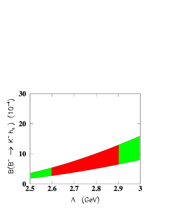
FIG. 2.: Branching fraction ${\cal B}(B^{-}\to K^{-}h_{c})$ versus the parameter $\Lambda$. The lowest curve corresponds to ${\rm Re}{\cal A}_{i}=0$, the highest one to ${\rm Re}{\cal A}_{i}={\rm Im}{\cal A}_{i}$. The dark region corresponds to the result (64).

REFERENCES

• [1] G. Buchalla, A. J. Buras and M. E. Lautenbacher, Rev. Mod. Phys.  68, 1125 (1996). A. J. Buras, arXiv:hep-ph/9806471.
• [2] M. Neubert and B. Stech, Adv. Ser. Direct. High Energy Phys.  15, 294 (1998).
• [3] M. Beneke, G. Buchalla, M. Neubert and C. T. Sachrajda, Nucl. Phys. B 591, 313 (2000).
• [4] Y. Y. Keum, H. n. Li and A. I. Sanda, Phys. Lett. B 504, 6 (2001).
• [5] C. W. Bauer, D. Pirjol and I. W. Stewart, Phys. Rev. Lett.  87, 201806 (2001).
• [6] B. Y. Blok and M. A. Shifman, Sov. J. Nucl. Phys.  45, 301 (1987) [Yad. Fiz.  45, 478 (1987)]; Sov. J. Nucl. Phys.  45, 522 (1987) [Yad. Fiz.  45, 841 (1987)].
• [7] More recent references can be found in the review: P. Colangelo and A. Khodjamirian, in At the Frontier of Particle Physics/Handbook of QCD, edited by M. A. Shifman (World Scientific, 2001) 1671 [arXiv:hep-ph/0010175].
• [8] P. Colangelo, F. De Fazio, P. Santorelli and E. Scrimieri, Phys. Rev. D 53, 3672 (1996) [Erratum-ibid. D 57, 3186 (1998)].
• [9] K. Abe et al. [Belle Collab.], Phys. Rev. Lett.  88, 031802 (2002).
• [10] B. Aubert et al. [BABAR Collaboration], arXiv:hep-ex/0207066.
• [11] H. Y. Cheng and K. C. Yang, Phys. Rev. D 63, 074011 (2001); Z. z. Song and K. T. Chao, Phys. Lett. B 568, 127 (2003).
• [12] P. Colangelo, F. De Fazio and T. N. Pham, Phys. Lett. B 542, 71 (2002).
• [13] N. N. Achasov and A. A. Kozhevnikov, Phys. Rev. D 49, 275 (1994).
• [14] M. Wanninger and L. M. Sehgal, Z. Phys. C 50, 47 (1991); A. N. Kamal, Int. J. Mod. Phys. A 7, 3515 (1992); Z. z. Xing, Phys. Lett. B 493, 301 (2000).
• [15] P. Colangelo, G. Nardulli, N. Paver and Riazuddin, Z. Phys. C 45, 575 (1990); C. Isola, M. Ladisa, G. Nardulli, T. N. Pham and P. Santorelli, Phys. Rev. D 64, 014029 (2001); C. Isola, M. Ladisa, G. Nardulli and P. Santorelli, arXiv:hep-ph/0307367.
• [16] The role of corrections to factorized amplitudes, among which rescattering terms are, is discussed in M. Ciuchini, E. Franco, G. Martinelli, M. Pierini and L. Silvestrini, Phys. Lett. B 515, 33 (2001) and in references therein.
• [17] D. Choudhury and J. R. Ellis, Phys. Lett. B 433, 102 (1998).
• [18] M. Diehl and G. Hiller, JHEP 0106, 067 (2001).
• [19] C. Baglin et al. [R704 Collaboration], Phys. Lett. B 171, 135 (1986).
• [20] T. A. Armstrong et al., Phys. Rev. Lett.  69, 2337 (1992).
• [21] L. Antoniazzi et al. [E705 Collaboration], Phys. Rev. D 50, 4258 (1994).
• [22] K. Hagiwara et al. [Particle Data Group Collaboration], Phys. Rev. D 66, 010001 (2002).
• [23] For reviews see: M. Neubert, Phys. Rept.  245, 259 (1994); F. De Fazio, in At the Frontier of Particle Physics/Handbook of QCD, edited by M. A. Shifman (World Scientific, 2001) 1671 [arXiv:hep-ph/0010007].
• [24] H. Georgi, Phys. Lett. B 240, 447 (1990).
• [25] Z. Luo and J. L. Rosner, Phys. Rev. D 64, 094001 (2001).
• [26] M. B. Wise, Phys. Rev. D 45, 2188 (1992); G. Burdman and J. F. Donoghue, Phys. Lett. B 280, 287 (1992); T. M. Yan et al., Phys. Rev. D 46, 1148 (1992) [Erratum-ibid. D 55, 5851 (1992)].
• [27] E. Jenkins, M. E. Luke, A. V. Manohar and M. J. Savage, Nucl. Phys. B 390, 463 (1993).
• [28] R. Casalbuoni, A. Deandrea, N. Di Bartolomeo, R. Gatto, F. Feruglio and G. Nardulli, Phys. Lett. B 309, 163 (1993).
• [29] O. Gortchakov, M. P. Locher, V. E. Markushin and S. von Rotz, Z. Phys. A 353, 447 (1996).
• [30] A. Anastassov et al. [CLEO Collab.], Phys. Rev. D 65, 032003 (2002).
• [31] The determination in T. N. Pham, Phys. Rev. D 25, 2955 (1982), based on current algebra arguments, is in agreement with the experimental result within the uncertainties. Most recent analyses of $g$ can be found in P. Colangelo and F. De Fazio, Phys. Lett. B 532, 193 (2002); F. S. Navarra, M. Nielsen and M. E. Bracco, Phys. Rev. D 65, 037502 (2002); A. Abada et al., Phys. Rev. D 66, 074504 (2002), while a list of previous studies is reported in [7].
• [32] R. D. Matheus, F. S. Navarra, M. Nielsen and R. Rodrigues da Silva, Phys. Lett. B 541, 265 (2002); A. Deandrea, G. Nardulli and A. D. Polosa, Phys. Rev. D 68, 034002 (2003).
• [33] M. Beneke, F. Maltoni and I. Z. Rothstein, Phys. Rev. D 59, 054003 (1999).
• [34] Y. P. Kuang, Phys. Rev. D 65, 094024 (2002).
• [35] M. Suzuki, Phys. Rev. D 66, 037503 (2002).
• [36] S. Godfrey and J. L. Rosner, Phys. Rev. D 66, 014012 (2002).
• [37] S. Godfrey and N. Isgur, Phys. Rev. D 32, 189 (1985).
• [38] K. Abe et al. [Belle Collaboration], arXiv:hep-ex/0307061.
Refer to caption