New formalism for QCD parton showers

Abstract:

We present a new formalism for parton shower simulation of QCD jets, which incorporates the following features: invariance under boosts along jet axes, improved treatment of heavy quark fragmentation, angular-ordered evolution with soft gluon coherence, more accurate soft gluon angular distributions, and better coverage of phase space. It is implemented in the new HERWIG++ event generator.

1 Introduction

The parton shower approximation has become a key component of a wide range of comparisons between theory and experiment in particle physics. Calculations of infrared-safe observables, i.e. those that are asymptotically insensitive to soft physics, can be performed in fixed-order perturbation theory, but the resulting final states consist of a few isolated partons, quite unlike the multihadron final states observed experimentally. One can attempt to identify isolated partons with hadronic jets, but then the energy flows within and between jets are not well represented.

At present, the only means of connecting few-parton states with the real world is via parton showers, which generate high-multiplicity partonic final states in an approximation that retains enhanced collinear and soft contributions to all orders. Such multiparton states can be interfaced to a hadronization model which does not require large momentum transfers in order to produce a realistic hadronic final state. Hadronization and detector corrections to the fixed-order predictions can then be computed, and the results have generally been found to be in satisfactory agreement with the data. Infrared-sensitive quantities such as hadron spectra and multiplicities have also been described successfully using parton showers. This increases confidence that similar techniques can be used to predict new physics signals and backgrounds in future experiments.

A crucial ingredient of modern parton showering algorithms is angular ordering, which ensures that important aspects of soft gluon coherence are included in an azimuthally-averaged form. The angular shower evolution variable [2] used in the event generator program HERWIG [3] is good for ensuring that angular ordering is built in from the outset, but the phase space is complicated and not invariant under any kind of boosts. Evolution in virtuality looks natural but then angular ordering must be imposed afterwards, as is done in PYTHIA [4].

In the present paper we investigate a new shower evolution formalism, based on an angular variable related to transverse momentum [5, 6, 7, 8]. The main aim is to retain the direct angular ordering of the shower while improving the Lorentz invariance of the evolution and simplifying the coverage of phase space, especially in the soft region. The new shower variables also permit a better treatment of heavy quark fragmentation, through evolution down to zero transverse momentum and the use of mass-dependent splitting functions, which eliminate the sharply-defined collinear “dead cones” seen in earlier angular-ordered treatments.

In the following section we define the new shower variables and their associated kinematics and dynamics, including the appropriate argument of the running coupling, the mass-dependent parton branching probability, and the shower evolution cutoff. The variables are defined slightly differently for initial- and final-state parton branching, and depend on the colour connection of the evolving parton, so we consider in subsequent sections the various possible configurations of colour flow between initial and final jets.

The formalism presented here is implemented in the new Monte Carlo event generator HERWIG++ [9]. Results for $e^{+}e^{-}$ annihilation and comparisons with LEP data will be presented shortly in a separate publication [10]. The formulae in the present paper could also be used to construct a matching scheme for next-to-leading order (NLO) QCD calculations and HERWIG++ parton showers, similar to that developed for HERWIG showers in [11, 12] and implemented in the MC@NLO event generator [13], or to improve schemes for combining parton showers with fixed-order matrix elements [14].

2 New variables for parton branching

2.1 Final-state quark branching

2.1.1 Kinematics

Consider parton branching in an outgoing (heavy) quark jet. Define the quark momentum after the $i$th gluon emission $q_{i-1}\to q_{i}+k_{i}$ (see fig. 1) as

$$q_{i}=\alpha_{i}p+\beta_{i}n+q_{\perp i}$$ (1)

where $p$ is the jet’s “parent parton” momentum ($p^{2}=m^{2}$, the on-shell quark mass-squared), $n$ is a lightlike “backward” 4-vector ($n^{2}=0$), and $q_{\perp i}$ is the transverse momentum ($q_{\perp i}^{2}=-{\mbox{\bf q}_{\perp}}_{i}^{2}$, $q_{\perp i}\cdot p=q_{\perp i}\cdot n=0$). Then

$$\beta_{i}={{{\mbox{\bf q}_{\perp}}_{i}^{2}+q_{i}^{2}-\alpha_{i}^{2}m^{2}}\over{2\alpha_{i}p\cdot n}}\;.$$ (2)

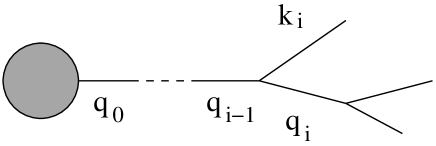
Figure 1: Final-state parton branching. The blob represents the hard subprocess.

The momentum fraction and relative transverse momentum are now defined as

$$z_{i}={{\alpha_{i}}\over{\alpha_{i-1}}}\;,\;\;\;\;\;\;{\mbox{\bf p}_{\perp i}}={\mbox{\bf q}_{\perp i}}-z_{i}\mbox{\bf q}_{\perp i-1}\;.$$ (3)

Then we have

$$q_{i-1}^{2}={{q_{i}^{2}}\over{z_{i}}}+{{k_{i}^{2}}\over{1-z_{i}}}+{{{\mbox{\bf p}_{\perp i}}^{2}}\over{z_{i}(1-z_{i})}}\;.$$ (4)

2.1.2 Running coupling

To find the optimal argument of $\alpha_{\mbox{\tiny S}}$, we consider the branching of a quark of virtuality $q^{2}$ into an on-shell quark and an off-shell gluon of virtuality $k^{2}$ [15]. From eq. (4), the propagator denominator is

$$q^{2}-m^{2}={{1-z}\over{z}}m^{2}+{{k^{2}}\over{1-z}}+{{{\mbox{\bf p}_{\perp}}^{2}}\over{z(1-z)}}={{1}\over{1-z}}\left\{k^{2}+{{1}\over{z}}[{\mbox{\bf p}_{\perp}}^{2}+(1-z)^{2}m^{2}]\right\}\;.$$ (5)

The dispersion relation for the running coupling is supposed to be

$${{\alpha_{\mbox{\tiny S}}(\mu^{2})}\over{\mu^{2}}}={{\alpha_{\mbox{\tiny S}}(0)}\over{\mu^{2}}}+\int_{0}^{\infty}{{dk^{2}}\over{k^{2}(k^{2}+\mu^{2})}}\rho_{\mbox{\tiny S}}(k^{2})$$ (6)

where $\rho_{\mbox{\tiny S}}(k^{2})$ is the discontinuity of $\alpha_{\mbox{\tiny S}}(-k^{2})$. The first term on the right-hand side comes from cutting through the on-shell gluon, the second from cutting through the gluon self-energy. In our case we have $k^{2}+[{\mbox{\bf p}_{\perp}}^{2}+(1-z)^{2}m^{2}]/z$ in place of $k^{2}+\mu^{2}$. We are interested in soft gluon resummation ($z\to 1$) [8] and so we ignore the factor of $1/z$ here. Thus the suggested argument of $\alpha_{\mbox{\tiny S}}$ is ${\mbox{\bf p}_{\perp}}^{2}+(1-z)^{2}m^{2}$. In practice we impose a minimum virtuality on light quarks and gluons in the parton shower, and therefore the actual argument is slightly more complicated (see below).

2.1.3 Evolution variable

The evolution variable is not simply $q^{2}$ since this would ignore angular ordering. For massless parton branching this means the evolution variable should be ${\mbox{\bf p}_{\perp}}^{2}/[z(1-z)]^{2}=q^{2}/z(1-z)$ [18]. For gluon emission by a massive quark we assume this generalizes to $(q^{2}-m^{2})/z(1-z)$. To define a resolvable emission we also need to introduce a minimum virtuality $Q_{g}^{2}$ for gluons and light quarks. Therefore from eq. (5) the evolution variable is

$$\tilde{q}^{2}={{{\mbox{\bf p}_{\perp}}^{2}}\over{z^{2}(1-z)^{2}}}+{{\mu^{2}}\over{z^{2}}}+{{Q_{g}^{2}}\over{z(1-z)^{2}}}$$ (7)

where $\mu=\max(m,Q_{g})$. For the argument of the running coupling we use

$$z^{2}(1-z)^{2}\tilde{q}^{2}={\mbox{\bf p}_{\perp}}^{2}+(1-z)^{2}\mu^{2}+zQ_{g}^{2}\;.$$ (8)

Note that for massive quarks this allows us to evolve down to ${\mbox{\bf p}_{\perp}}<(1-z)m$, i.e. inside the dead cone [16, 17].

Angular ordering of the branching $q_{i}\to q_{i+1}$ is defined by

$$\tilde{q}_{i+1}<z_{i}\tilde{q}_{i}\;.$$ (9)

The factor of $z_{i}$ enters because the angle at each branching is inversely proportional to the momentum fraction of the parent. Similarly for branching on the gluon, $k_{i}\to k_{i+1}$, we require

$$\tilde{k}_{i+1}<(1-z_{i})\tilde{q}_{i}\;.$$ (10)

2.1.4 Branching probability

For the parton branching probability we use the mass-dependent splitting functions of ref. [7]. These are derived in the quasi-collinear limit, in which ${\mbox{\bf p}_{\perp}}^{2}$ and $m^{2}$ are treated as small (compared to $p\cdot n$) but ${\mbox{\bf p}_{\perp}}^{2}/m^{2}$ is not necessarily small. In this limit the $q\to qg$ splitting function is

$$P_{qq}(z,{\mbox{\bf p}_{\perp}}^{2})=C_{F}\left[{{1+z^{2}}\over{1-z}}-{{2z(1-z)m^{2}}\over{{\mbox{\bf p}_{\perp}}^{2}+(1-z)^{2}m^{2}}}\right]\;.$$ (11)

Note that at ${\mbox{\bf p}_{\perp}}=0$ the factor in square brackets is just $1-z$, i.e. the soft singularity at $z\to 1$ becomes a zero in the collinear direction. The minimum virtuality $Q_{g}^{2}$ serves only to define a resolvable emission, and therefore we omit it when defining the branching probability in terms of the evolution variable (7) as

$$dP(q\to qg)={{\alpha_{\mbox{\tiny S}}}\over{2\pi}}{{d\tilde{q}^{2}}\over{\tilde{q}^{2}}}\,P_{qq}\,dz={{C_{F}}\over{2\pi}}\alpha_{\mbox{\tiny S}}[z^{2}(1-z)^{2}\tilde{q}^{2}]{{d\tilde{q}^{2}}\over{\tilde{q}^{2}}}{{dz}\over{1-z}}\left[1+z^{2}-{{2m^{2}}\over{z\tilde{q}^{2}}}\right]\;.$$ (12)

2.2 Gluon splitting

In the case of a final-state gluon splitting into a pair of heavy quarks of mass $m$, the quasi-collinear splitting function derived in [7] is

$$P_{qg}(z,{\mbox{\bf p}_{\perp}}^{2})=T_{R}\left[1-2z(1-z){{{\mbox{\bf p}_{\perp}}^{2}}\over{{\mbox{\bf p}_{\perp}}^{2}+m^{2}}}\right]\,.$$ (13)

We note that this splitting function is bounded above by its value $T_{R}=\mbox{\small${{1}\over{2}}$}$ at the phase space boundary ${\mbox{\bf p}_{\perp}}={\mbox{\bf 0}}$, and below by $T_{R}/2$. By analogy with eq. (7), in this case the evolution variable $\tilde{q}$ is related to the virtuality of the gluon or the relative transverse momentum of the splitting by

$$\tilde{q}^{2}={{q^{2}}\over{z(1-z)}}={{{\mbox{\bf p}_{\perp}}^{2}+m^{2}}\over{z^{2}(1-z)^{2}}}\,.$$ (14)

In terms of the variables $\tilde{q},z$, the $g\to q{\bar{q}}$ branching probability then reads

$$dP(g\to q{\bar{q}})={{T_{R}}\over{2\pi}}\alpha_{\mbox{\tiny S}}[z^{2}(1-z)^{2}\tilde{q}^{2}]{{d\tilde{q}^{2}}\over{\tilde{q}^{2}}}\left[1-2z(1-z)+{{2m^{2}}\over{z(1-z)\tilde{q}^{2}}}\right]\,dz\,.$$ (15)

In the case of gluon splitting into gluons, the branching probability takes the familiar form

$$dP(g\to gg)={{C_{A}}\over{2\pi}}\alpha_{\mbox{\tiny S}}[z^{2}(1-z)^{2}\tilde{q}^{2}]{{d\tilde{q}^{2}}\over{\tilde{q}^{2}}}\left[{{z}\over{1-z}}+{{1-z}\over{z}}+z(1-z)\right]\,dz\,.$$ (16)

Since we introduce a minimum virtuality $Q_{g}^{2}$ for gluons, the relationship between the evolution variable and the relative transverse momentum for this splitting is as in eq. (14) but with the heavy quark mass $m$ replaced by $Q_{g}$. Similarly, for gluon splitting to light quarks we use eq. (14) with $\mu=\max(m,Q_{g})$ in place of $m$.

2.3 Initial-state branching

Consider the initial-state (spacelike) branching of a partonic constituent of an incoming hadron that undergoes some hard collisions subprocess such as deep inelastic lepton scattering. The momenta are defined as in eq. (1), with the reference vector $p$ along the beam direction. In this case the evolution is performed backwards from the hard sub-process to the incoming hadron, as shown in fig. 2.

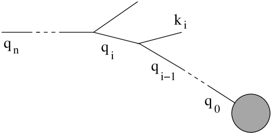
Figure 2: Initial-state parton branching. The blob represents the hard subprocess.

Thus we now define in place of eq. (3)

$$z_{i}={{\alpha_{i-1}}\over{\alpha_{i}}}\;,\;\;\;\;\;\;{\mbox{\bf p}_{\perp i}}={\mbox{\bf q}_{\perp i-1}}-z_{i}{\mbox{\bf q}_{\perp i}}\;.$$ (17)

Then

$$q_{i-1}^{2}=z_{i}q_{i}^{2}-{{z_{i}}\over{1-z_{i}}}k_{i}^{2}-{{{\mbox{\bf p}_{\perp i}}^{2}}\over{1-z_{i}}}\;.$$ (18)

We assume a massless variable-flavour-number evolution scheme [19, 20] for constituent parton branching, setting $m=0$ and putting all emitted gluons at the minimum virtuality, $k_{i}^{2}=Q_{g}^{2}$. The angular evolution variable now relates only to the angle of the emitted gluon and therefore we choose

$$\tilde{q}_{i}^{2}={{{\mbox{\bf p}_{\perp i}}^{2}+z_{i}Q_{g}^{2}}\over{(1-z_{i})^{2}}}\;,$$ (19)

with ordering condition simply $\tilde{q}_{i+1}<\tilde{q}_{i}$. Correspondingly, for the argument of the running coupling we now use $(1-z)^{2}\tilde{q}^{2}$.

A different type of initial-state branching occurs in the decay of heavy, quasi-stable coloured objects like the top quark. Here the momentum of the incoming heavy object is fixed and evolution is performed forwards to the hard decay process. In this case we cannot neglect the mass of the parton and eq. (19) becomes

$$\tilde{q}_{i}^{2}={{{\mbox{\bf p}_{\perp i}}^{2}+z_{i}Q_{g}^{2}}\over{(1-z_{i})^{2}}}+m^{2}\;,$$ (20)

while the branching probability (12) is replaced by

$$dP(q\to qg)={{C_{F}}\over{2\pi}}\alpha_{\mbox{\tiny S}}[(1-z)^{2}\tilde{q}^{2}]{{d\tilde{q}^{2}}\over{\tilde{q}^{2}}}{{dz}\over{1-z}}\left[1+z^{2}-{{2zm^{2}}\over{\tilde{q}^{2}}}\right]\;.$$ (21)

2.4 Allowed regions and termination of branching

The allowed phase space for each branching is given by requiring a real relative transverse momentum, ${\mbox{\bf p}_{\perp}}^{2}>0$. In final-state $q\to qg$ branching, we have from eq. (8)

$$z^{2}(1-z)^{2}\tilde{q}^{2}>(1-z)^{2}\mu^{2}+zQ_{g}^{2}\;.$$ (22)

This yields a rather complicated boundary in the $(\tilde{q},z)$ plane. However, since

$$(1-z)^{2}\mu^{2}+zQ_{g}^{2}>(1-z)^{2}\mu^{2}\,,\;z^{2}Q_{g}^{2}$$ (23)

we see that the phase space lies inside the region

$${{m}\over{\tilde{q}}}<z<1-{{Q_{g}}\over{\tilde{q}}}\;,$$ (24)

and approaches these limits for large values of $\tilde{q}$. The precise phase space can therefore be filled efficiently by generating values of $z$ between these limits and rejecting those that violate the inequality (22). The resulting threshold for $\tilde{q}$ is slightly larger than but of the order of $m+Q_{g}$.

In gluon splitting, we obtain the allowed phase space range from eq. (14) as

$$z_{-}<z<z_{+},\qquad z_{\pm}={{1}\over{2}}\left(1\pm\sqrt{1-{{4\mu}\over{\tilde{q}}}}\right)\qquad\mathrm{and}\quad\tilde{q}>4\mu$$ (25)

where $\mu=m$ for splitting into heavy quarks, or $\mu=\max(m,Q_{g})$ more generally. Therefore, analogously to eq. (24), the phase space lies within the range

$${{\mu}\over{\tilde{q}}}<z<1-{{\mu}\over{\tilde{q}}}\;.$$ (26)

Schematically, the parton shower corresponds to selecting a sequence of $(\tilde{q}_{i},z_{i})$ values by solving the equations

$$R_{1} = \exp\left(-\int_{\tilde{q}_{i}}^{\tilde{q}_{i-1}}d\tilde{q}\int_{z_{-}}^{z_{+}}dz\,{{d^{2}P}\over{d\tilde{q}\,dz}}\right)$$

$$R_{2} = \int_{z_{-}}^{z_{i}}dz\,{{d^{2}P}\over{d\tilde{q}\,dz}}\Bigg{/}\int_{z_{-}}^{z_{+}}dz\,{{d^{2}P}\over{d\tilde{q}\,dz}}$$ (27)

where $R_{1,2}\in[0,1]$ are uniform pseudorandom numbers. Whenever the algorithm selects a value of $\tilde{q}$ below the threshold, branching of that parton is terminated. The minimum virtuality $Q_{g}$ thus determines the scale at which soft or collinear parton emission becomes unresolvable. In the absence of such a scale one eventually reaches a region where the perturbative expression for the running coupling is divergent.

One may wish to use a parametrization of $\alpha_{\mbox{\tiny S}}$ at low scales such that $\alpha_{\mbox{\tiny S}}(0)$ is finite. However, a cutoff $Q_{g}$ is still needed to avoid divergence of the $q\to qg$ and $g\to gg$ branching probabilities. Alternatively one could consider parametrizing $\alpha_{\mbox{\tiny S}}$ such that $\alpha_{\mbox{\tiny S}}(0)=0$, e.g.

$$\alpha_{\mbox{\tiny S}}(q^{2})={{q}\over{Q_{c}}}\alpha_{\mbox{\tiny S}}(Q_{c}^{2})\;\;\;\;\mbox{for}\;q<Q_{c}\;,$$ (28)

where $Q_{c}>\Lambda$. Then the total branching probability below $Q_{c}$ is (for massless quarks)

$$P_{c}(q\to qg)=C_{F}{{\alpha_{\mbox{\tiny S}}(Q_{c}^{2})}\over{2\pi}}\int_{0}^{1}2z(1+z^{2})\,dz={{\alpha_{\mbox{\tiny S}}(Q_{c}^{2})}\over{\pi}}\;,$$ (29)

and no explicit cutoff is required, although of course $Q_{c}$ is essentially playing the same rôle.

After branching has terminated, the outgoing partons are put on mass-shell (or given the virtual mass $Q_{g}$ if lighter) and the relative transverse momenta of the branchings in the shower are computed. For final-state gluon splitting we have

$$|{\mbox{\bf p}_{\perp}}|=\sqrt{z^{2}(1-z)^{2}\tilde{q}^{2}-\mu^{2}},$$ (30)

or else, if the parent is a quark,

$$|{\mbox{\bf p}_{\perp}}|=\sqrt{(1-z)^{2}(z^{2}\tilde{q}^{2}-\mu^{2})-zQ_{g}^{2}}.$$ (31)

The virtualities of the internal lines of the shower can now be computed backwards according to eq. (4). Finally, the azimuthal directions of the ${\mbox{\bf p}_{\perp}}$’s can be chosen [21] and the full 4-momenta reconstructed using eqs. (1) and (2).

In initial-state constituent parton branching the evolution is “guided” by the parton distribution functions (PDFs) of the incoming parent hadron. Since PDFs are often not tabulated below some scale $Q_{s}>Q_{0}$, one may wish to terminate branching whenever $\tilde{q}<Q_{s}$ is selected. In that case the incoming parton is assigned virtuality $q_{n}^{2}\sim-Q_{s}^{2}$ and the spacelike virtualities of internal lines are then reconstructed back from $q_{n}^{2}$ to $q_{0}^{2}$ using the transverse momenta deduced from eq. (19) inserted in eq. (18).

For initial-state branching in the decay of a heavy, quasi-stable coloured object, the branching proceeds in the opposite direction but the reconstruction of momenta is similar, using eq. (20) instead of (19).

2.5 Treatment of colour flows

The more detailed treatment depend on the choice of the “backward” vector $n$ and on which quantities are to be held fixed during jet evolution. Normally $n$ should be taken along the colour-connected partner of the radiating parton, and the 4-momentum of the colour-connected system should be preserved. The upper limits on the evolution variable $\tilde{q}$ for the colour-connected jets should be chosen so as to cover the phase space in the soft limit, with the best possible approximation to the correct angular distribution. In setting these limits we neglect the minimum virtuality $Q_{g}^{2}$, which is a good approximation at high energies. We consider separately the four cases that the colour connection is between two final-state jets, two initial-state (beam) jets, a beam jet and a final-state jet, or a decaying heavy parton and a decay-product jet.

3 Final-final colour connection

Consider the process $a\to b+c$ where $a$ is a colour singlet and $b$ and $c$ are colour-connected. Examples are $e^{+}e^{-}\to q{\bar{q}}$ and $W\to q{\bar{q}}^{\prime}$. We need to preserve the 4-momentum of $a$ and therefore we work in its rest-frame,

$$p_{a}=Q(1,{\mbox{\bf 0}},0)\;,\;\;\;p_{b}=\mbox{\small${{1}\over{2}}$}Q(1+b-c,{\mbox{\bf 0}},\lambda)\;,\;\;\;p_{c}=\mbox{\small${{1}\over{2}}$}Q(1-b+c,{\mbox{\bf 0}},-\lambda)\;,$$ (32)

where $p_{a}^{2}=Q^{2}$, $b=m_{b}^{2}/Q^{2}$, $c=m_{c}^{2}/Q^{2}$ and

$$\lambda=\lambda(1,b,c)\equiv\sqrt{(1+b-c)^{2}-4b}=\sqrt{(1-b+c)^{2}-4c}\;.$$ (33)

For emission of a gluon $g$ from $b$ we write

$$q_{i}=\alpha_{i}p_{b}+\beta_{i}n+q_{\perp i}$$ (34)

where ${\mbox{\bf q}_{\perp g}}={\mbox{\bf k}_{\perp}}$, ${\mbox{\bf q}_{\perp b}}=-{\mbox{\bf k}_{\perp}}$, ${\mbox{\bf q}_{\perp c}}={\mbox{\bf 0}}$ and we choose

$$n=\mbox{\small${{1}\over{2}}$}Q(\lambda,{\mbox{\bf 0}},-\lambda)\;.$$ (35)

Notice that, if $c$ is massive, the alignment of $n$ along $p_{c}$ is exact only in a certain class of Lorentz frames. However, if we try to use a massive “backward” vector the kinematics become too complicated.

To preserve $p_{a}=q_{b}+q_{c}+q_{g}$ we require

$$\sum\alpha_{i}=\sum\beta_{i}={{2}\over{1+b-c+\lambda}}$$ (36)

whereas the mass-shell conditions give

$$\beta_{b} = {{2}\over{\lambda(1+b-c+\lambda)}}\left({{b+\kappa}\over{\alpha_{b}}}-b\alpha_{b}\right)$$

$$\beta_{c} = {{2}\over{\lambda(1+b-c+\lambda)}}\left({{c}\over{\alpha_{c}}}-b\alpha_{c}\right)$$ (37)

$$\beta_{g} = {{2}\over{\lambda(1+b-c+\lambda)}}\left({{\kappa}\over{\alpha_{g}}}-b\alpha_{g}\right)$$

where $\kappa\equiv{\mbox{\bf k}_{\perp}}^{2}/Q^{2}$. Our new variables are

$$z={{\alpha_{b}}\over{\alpha_{b}+\alpha_{g}}}\;,\;\;\;\tilde{\kappa}\equiv{{\tilde{q}^{2}}\over{Q^{2}}}>b\;,$$ (38)

where from eq. (7) we have

$$\kappa=(z^{2}\tilde{\kappa}-b)(1-z)^{2}\;,$$ (39)

and so $\sqrt{b/\tilde{\kappa}}<z<1$. From eqs.(36)-(39) we find

$$\alpha_{b} = {{z}\over{1+b-c+\lambda}}\left(1+b-c+z(1-z)\tilde{\kappa}+\sqrt{[1-b+c-z(1-z)\tilde{\kappa}]^{2}-4b}\right)\;,$$

$$\alpha_{c} = {{2}\over{1+b-c+\lambda}}-{{\alpha_{b}}\over{z}}\;,$$ (40)

$$\alpha_{g} = {{1-z}\over{z}}\alpha_{b}\;,$$

with the $\beta_{i}$’s given by eq. (3).

3.1 Phase space variables

It is convenient to express the phase space in terms of the Dalitz plot variables

$$x_{i}={{2p_{a}\cdot q_{i}}\over{Q^{2}}}=(1+b-c)\alpha_{i}+\lambda\beta_{i}\;.$$ (41)

Substituting from eqs. (3) and (3), we find

$$x_{c} = 1-b+c-z(1-z)\tilde{\kappa}$$

$$x_{b} = (2-x_{c})r+(z-r)\sqrt{x_{c}^{2}-4c}$$ (42)

$$x_{g} = (2-x_{c})(1-r)-(z-r)\sqrt{x_{c}^{2}-4c}$$

where

$$r={{1}\over{2}}\left(1+{{b}\over{1+c-x_{c}}}\right)\;.$$ (43)

The Jacobian factor is thus simply

$${{\partial(x_{b},x_{c})}\over{\partial(z,\tilde{\kappa})}}=z(1-z)\sqrt{x_{c}^{2}-4c}$$ (44)

and the quasi-collinear branching probability (12) translates to

$$dP(q\to qg)=C_{F}{{\alpha_{\mbox{\tiny S}}}\over{2\pi}}{{dx_{b}\,dx_{c}}\over{(1-b+c-x_{c})\sqrt{x_{c}^{2}-4c}}}\left[{{1+z^{2}}\over{1-z}}-{{2b}\over{1-b+c-x_{c}}}\right]$$ (45)

where

$$z=r+{{x_{b}-(2-x_{c})r}\over{\sqrt{x_{c}^{2}-4c}}}\;,$$ (46)

$r$ being the function of $x_{c}$ given in eq. (43).

For emission from parton $c$ we write

$$q_{i}=\alpha_{i}p_{c}+\beta_{i}n+q_{\perp i}$$ (47)

where now we choose

$$n=\mbox{\small${{1}\over{2}}$}Q(\lambda,{\mbox{\bf 0}},\lambda)\;.$$ (48)

Clearly, the region covered and the branching probability will be as for emission from parton $b$, but with $x_{b}$ and $x_{c}$, $b$ and $c$ interchanged.

3.2 Soft gluon region

For emission from parton $b$ in the soft region $1-z=\epsilon\to 0$ we have

$$x_{c}\sim 1-b+c-\epsilon\tilde{\kappa}\;,\;\;\;x_{b}\sim 1+b-c-\epsilon\tilde{\kappa}^{\prime}$$ (49)

where

$$\tilde{\kappa}^{\prime}=\lambda+{{\tilde{\kappa}}\over{2b}}(1-b-c-\lambda)\;.$$ (50)

Since $\tilde{\kappa}$ is an angular variable, we can express it in terms of the angle $\theta_{bg}$ between the directions of the emitting parton $b$ and the emitted gluon in the rest frame of $a$. In the soft region we find

$$\tilde{\kappa}={{(1+b-c+\lambda)(1+b-c-\lambda\cos\theta_{bg})}\over{2(1+\cos\theta_{bg})}}$$ (51)

Thus $\tilde{\kappa}=b$ at $\theta_{bg}=0$ and $\tilde{\kappa}\to\infty$ as $\theta_{bg}\to\pi$.

For soft emission from parton $c$, the roles of $x_{b}$ and $x_{c}$, $b$ and $c$ are interchanged. To cover the whole angular region in the soft limit, we therefore require $\tilde{\kappa}<\tilde{\kappa}_{b}$ in jet $b$ and $\tilde{\kappa}<\tilde{\kappa}_{c}$ in jet $c$, where

$${{\tilde{\kappa}_{b}}\over{\tilde{\kappa}^{\prime}_{b}}}={{\tilde{\kappa}^{\prime}_{c}}\over{\tilde{\kappa}_{c}}}$$ (52)

and hence

$$(\tilde{\kappa}_{b}-b)(\tilde{\kappa}_{c}-c)={{1}\over{4}}(1-b-c+\lambda)^{2}\;.$$ (53)

In particular, the most symmetric choice is

$$\tilde{\kappa}_{b}=\mbox{\small${{1}\over{2}}$}(1+b-c+\lambda)\;,\;\;\;\tilde{\kappa}_{c}=\mbox{\small${{1}\over{2}}$}(1-b+c+\lambda)\;.$$ (54)

The largest region that can be covered by one jet corresponds to the maximal value of $\tilde{\kappa}$ allowed in eq. (3) for real $\alpha_{b}$, i.e. for the maximal $b$ jet

$$\tilde{\kappa}_{b}=4(1-2\sqrt{b}-b+c)\;.$$ (55)

3.3 Example: $e^{+}e^{-}\to q\bar{q}g$

Here we have $b=c=\rho$, $\lambda=\sqrt{1-4\rho}=v$, the quark velocity in the Born process $e^{+}e^{-}\to q\bar{q}$. The phase space and the two jet regions for the symmetrical choice (54) are shown in fig. 3. The region D, corresponding to hard non-collinear gluon emission, is not included in either jet and must be filled using the ${\cal O}(\alpha_{\mbox{\tiny S}})$ matrix element (see below).

Figure 3: Phase space for $e^{+}e^{-}\to q{\bar{q}}g$ for $m_{q}=5$ GeV, $Q^{2}=m_{Z}^{2}$, with symmetric definition of quark and antiquark jets.

For the maximal quark jet we get from eq. (55)

$$\tilde{\kappa}_{q}=4(1-2\sqrt{\rho})\;,$$ (56)

as shown in fig. 4 together with the complementary antiquark jet region given by eq. (53).

Figure 4: Phase space for $e^{+}e^{-}\to q{\bar{q}}g$ for $m_{q}=5$ GeV, $Q^{2}=m_{Z}^{2}$, with maximal region for the quark jet.

3.3.1 Exact matrix element

The $e^{+}e^{-}\to V\to q{\bar{q}}g$ differential cross section, where $V$ represents a vector current such as a virtual photon, is given to first order in $\alpha_{\mbox{\tiny S}}$ by [22, 23]

$${{1}\over{\sigma_{V}}}{{d^{2}\sigma_{V}}\over{dx_{q}\,dx_{\bar{q}}}}={{\alpha_{\mbox{\tiny S}}}\over{2\pi}}{{C_{F}}\over{v}}\left[{{(x_{q}+2\rho)^{2}+(x_{\bar{q}}+2\rho)^{2}+\zeta_{V}}\over{(1+2\rho)(1-x_{q})(1-x_{\bar{q}})}}-{{2\rho}\over{(1-x_{q})^{2}}}-{{2\rho}\over{(1-x_{\bar{q}})^{2}}}\right]$$ (57)

where

$$\zeta_{V}=-8\rho(1+2\rho)$$ (58)

and

$$\sigma_{V}=\sigma_{0}\left(1+2\rho\right)v$$ (59)

is the Born cross section for heavy quark production by a vector current, $\sigma_{0}$ being the massless quark Born cross section.

In the case of the axial current contribution $e^{+}e^{-}\to A\to q{\bar{q}}g$, instead of eq. (57) we have

$${{1}\over{\sigma_{A}}}{{d^{2}\sigma_{A}}\over{dx_{q}\,dx_{\bar{q}}}}={{\alpha_{\mbox{\tiny S}}}\over{2\pi}}{{C_{F}}\over{v}}\left[{{(x_{q}+2\rho)^{2}+(x_{\bar{q}}+2\rho)^{2}+\zeta_{A}}\over{v^{2}(1-x_{q})(1-x_{\bar{q}})}}-{{2\rho}\over{(1-x_{q})^{2}}}-{{2\rho}\over{(1-x_{\bar{q}})^{2}}}\right]\;,$$ (60)

where

$$\zeta_{A}=2\rho[(3+x_{g})^{2}-19+4\rho]\;,$$ (61)

$\sigma_{A}$ being the Born cross section for heavy quark production by the axial current:

$$\sigma_{A}=\sigma_{0}v^{3}\;.$$ (62)

3.3.2 Soft gluon distribution

In the soft gluon region $1-z=\epsilon\to 0$ the branching probability (45) becomes

$${{d^{2}P}\over{dx_{q}\,dx_{\bar{q}}}} \sim {{\alpha_{\mbox{\tiny S}}}\over{2\pi}}{{2C_{F}}\over{v\epsilon^{2}}}f_{s}(\tilde{\kappa})$$

$$f_{s}(\tilde{\kappa}) = {{1}\over{\tilde{\kappa}}}-{{\rho}\over{\tilde{\kappa}^{2}}}\;.$$ (63)

In this limit, the exact vector and axial current matrix elements, eqs. (57) and (60) respectively, give identical distributions:

$${{1}\over{\sigma_{V}}}{{d^{2}\sigma_{V}}\over{dx_{q}\,dx_{\bar{q}}}} \sim {{1}\over{\sigma_{A}}}{{d^{2}\sigma_{A}}\over{dx_{q}\,dx_{\bar{q}}}}\sim{{\alpha_{\mbox{\tiny S}}}\over{2\pi}}{{2C_{F}}\over{v\epsilon^{2}}}f(\tilde{\kappa})$$

$$f(\tilde{\kappa}) = {{1-2\rho}\over{\tilde{\kappa}\tilde{\kappa}^{\prime}}}-{{\rho}\over{\tilde{\kappa}^{2}}}-{{\rho}\over{\tilde{\kappa}^{\prime 2}}}$$ (64)

$$= f_{s}(\tilde{\kappa})\left({{v}\over{\tilde{\kappa}^{\prime}}}\right)^{2}\;.$$

Since from eq. (50)

$$\tilde{\kappa}^{\prime}=v+\tilde{\kappa}\left({{1-v}\over{1+v}}\right)>v\;,$$ (65)

the parton shower approximation (3.3.2) always overestimates the true result in the soft limit, and so correction by the rejection method is straightforward. For small values of $\rho$ we have

$$f(\tilde{\kappa})={{1}\over{\tilde{\kappa}}}-{{\rho}\over{\tilde{\kappa}^{2}}}+{{2\rho^{2}}\over{\tilde{\kappa}}}-2\rho+{\cal O}(\rho^{2})\;.$$ (66)

Since $\tilde{\kappa}>\rho$ we see that the error in the approximation (3.3.2) is at most ${\cal O}(\rho)$, for any value of $\tilde{\kappa}$ (fig. 5).

Figure 5: The function $f(\tilde{\kappa})$ giving the gluon angular distribution in the soft limit, for $m=5$ GeV, $Q^{2}=m_{Z}^{2}$. The exact result eq. (3.3.2), solid curve, and shower approximation (3.3.2), dashed, are not distinguishable on this scale.

3.3.3 Dead region contribution

The integral over the dead region may be expressed as

$${{1}\over{\sigma_{V}}}\int_{D}d^{2}\sigma_{V}\equiv{{\alpha_{\mbox{\tiny S}}}\over{2\pi}}C_{F}\,F^{D}_{V}(\tilde{\kappa}_{q})$$ (67)

where $\tilde{\kappa}_{q}$ parametrizes the boundary of the quark jet. As shown in fig. 6, this is actually maximal, but still small, at the symmetric point given by eq. (54).

Figure 6: The function $F^{D}(\tilde{\kappa}_{q})$ giving the contribution of the dead region to the cross section, for $m=5$ GeV, $Q^{2}=m_{Z}^{2}$. Solid: vector current. Dashed: axial current.

Although the integral in eq. (67) is finite, the integrand diverges as one approaches the soft limit $x_{q}=x_{\bar{q}}=1$ via the narrow “neck” of the dead region in fig. 3 or 4. This could cause problems in generating $q{\bar{q}}g$ configurations in the dead region in order to apply a matrix element correction [24]. To avoid such problems, one can map the region $x_{q},x_{\bar{q}}>{{3}\over{4}}$ into a region whose width vanishes quadratically as $x_{q},x_{\bar{q}}\to 1$, as illustrated in fig. 7.

Figure 7: The soft region, with jet boundaries (solid) and mapped region (dashed), for $m=5$ GeV, $Q^{2}=m_{Z}^{2}$.

The mapping shown is

$$x_{q}\to x^{\prime}_{q} = 1-\left[{{1}\over{4}}-(1-x_{q})\right]={{7}\over{4}}-x_{q}\;,$$

$$x_{\bar{q}}\to x^{\prime}_{\bar{q}} = 1-2(1-x^{\prime}_{q})\left[{{3}\over{4}}-(1-x_{q})\right]={{5}\over{8}}+{{1}\over{2}}x_{q}+{{3}\over{2}}x_{\bar{q}}-2x_{q}x_{\bar{q}}$$ (68)

when $x_{q}>x_{\bar{q}}>{{3}\over{4}}$. Within the mapped region, the integrand then has an extra weight factor of $2(1-x^{\prime}_{q})$ which regularizes the soft divergence. When $x_{\bar{q}}>x_{q}>{{3}\over{4}}$, $x_{q}$ and $x_{\bar{q}}$ are interchanged in both the mapping and the weight.

4 Initial-initial colour connection

Here we consider the inverse process $b+c\to a$ where $a$ is a colour singlet of invariant mass $Q$ and $b,c$ are beam jets. The kinematics are simple because we take beam jets to be massless: in the c.m. frame

$$p_{a}=Q(1,{\mbox{\bf 0}},0)\;,\;\;\;p_{b}=\mbox{\small${{1}\over{2}}$}Q(1,{\mbox{\bf 0}},1)\;,\;\;\;p_{c}=\mbox{\small${{1}\over{2}}$}Q(1,{\mbox{\bf 0}},-1)\;.$$ (69)

For emission of a gluon $g$ from $b$ we write

$$q_{i}=\alpha_{i}p_{b}+\beta_{i}p_{c}+q_{\perp i}$$ (70)

where ${\mbox{\bf q}_{\perp g}}={\mbox{\bf k}_{\perp}}$, ${\mbox{\bf q}_{\perp a}}=-{\mbox{\bf k}_{\perp}}$, ${\mbox{\bf q}_{\perp b}}={\mbox{\bf q}_{\perp c}}={\mbox{\bf 0}}$. Notice that in this case the recoil transverse momentum is taken by the colour singlet $a$ so we cannot preserve its 4-momentum. We choose to preserve its mass and rapidity, so that

$$\alpha_{a}=\beta_{a}=\sqrt{1+\kappa}\;,$$ (71)

where as before $\kappa\equiv{\mbox{\bf k}_{\perp}}^{2}/Q^{2}$. Now we have

$$\beta_{b} = \alpha_{c}=0\;,\;\;\;\alpha_{g}\beta_{g}=\kappa\;,$$

$$\alpha_{a} = \alpha_{b}-\alpha_{g}\;,\;\;\;\beta_{a}=\beta_{c}-\beta_{g}\;,$$ (72)

and our new variables in this case are

$$z=1-{{\alpha_{g}}\over{\alpha_{b}}}\;,\;\;\;\tilde{\kappa}\equiv{{\tilde{q}^{2}}\over{Q^{2}}}={{\kappa}\over{(1-z)^{2}}}\;.$$ (73)

Thus we find

$$\alpha_{a} = \beta_{a}=\sqrt{1+(1-z)^{2}\tilde{\kappa}}\;,$$

$$\alpha_{b} = {{1}\over{z}}\sqrt{1+(1-z)^{2}\tilde{\kappa}}\;,$$

$$\beta_{c} = {{1+(1-z)\tilde{\kappa}}\over{\sqrt{1+(1-z)^{2}\tilde{\kappa}}}}\;.$$ (74)

4.1 Phase space variables

It is convenient to express the kinematics in terms of the “reduced” Mandelstam invariants:

$${\bar{s}}=(q_{b}+q_{c})^{2}/Q^{2}\;,\;\;\;{\bar{t}}=(q_{b}-q_{g})^{2}/Q^{2}\;,\;\;\;{\bar{u}}=(q_{c}-q_{g})^{2}/Q^{2}\;.$$ (75)

The phase space limits are

$$1<{\bar{s}}<S/Q^{2}\;,\;\;\;1-{\bar{s}}<{\bar{t}}<0\;,\;\;\;{\bar{u}}=1-{\bar{s}}-{\bar{t}}$$ (76)

where $S$ is the beam-beam c.m. energy squared. In terms of the shower variables for beam jet $b$, we have

$${\bar{s}}=\alpha_{b}\beta_{c}={{1}\over{z}}[1+(1-z)\tilde{\kappa}]\;,\;\;\;{\bar{t}}=-\alpha_{b}\beta_{g}=-(1-z)\tilde{\kappa}\;,\;\;\;{\bar{u}}=-(1-z){\bar{s}}\;.$$ (77)

Thus curves of constant $\tilde{\kappa}$ in the $({\bar{s}},{\bar{t}})$ plane are given by

$${\bar{t}}={{\tilde{\kappa}(1-{\bar{s}})}\over{\tilde{\kappa}+{\bar{s}}}}$$ (78)

and the Jacobian factor for conversion of the shower variables to the Mandelstam invariants is

$${{\partial({\bar{s}},{\bar{t}})}\over{\partial(z,\tilde{\kappa})}}={{1-z}\over{z}}{\bar{s}}\;.$$ (79)

For the other beam jet $c$ we have ${\bar{t}}\leftrightarrow{\bar{u}}$ and thus

$${\bar{t}}={{{\bar{s}}(1-{\bar{s}})}\over{\tilde{\kappa}+{\bar{s}}}}\;.$$ (80)

We see that in order for the jet regions to touch without overlapping in the soft limit ${\bar{s}}\to 1$, ${\bar{t}}\to 0$, we need $\tilde{\kappa}<\tilde{\kappa}_{b}$ in jet $b$ and $\tilde{\kappa}<\tilde{\kappa}_{c}$ in jet $c$, where $\tilde{\kappa}_{c}=1/\tilde{\kappa}_{b}$. The most symmetrical choice is $\tilde{\kappa}_{c}=\tilde{\kappa}_{b}=1$, as shown in fig. 8, but we can take $\tilde{\kappa}_{b}$ or $\tilde{\kappa}_{c}$ as large as we like.

Figure 8: Beam jets (B,C) and dead region (D) in initial-state branching.

4.2 Example: Drell-Yan process

Consider radiation from the quark in the Drell-Yan process, $q\bar{q}\to gZ^{0}$. In the laboratory frame we have

$$q_{q}=(Px_{1},{\mbox{\bf 0}},Px_{1})\;,\;\;\;q_{{\bar{q}}}=(Px_{2},{\mbox{\bf 0}},-Px_{2})$$ (81)

where $P=\mbox{\small${{1}\over{2}}$}\sqrt{S}$ is the beam momentum. If we generated the initial hard process $q\bar{q}\to Z^{0}$ with momentum fractions $x_{q}$, $x_{\bar{q}}$ and we want to preserve the mass and rapidity of the $Z^{0}$ we require

$$x_{1}=x_{q}\alpha_{b}\;,\;\;\;x_{2}=x_{\bar{q}}\beta_{c}$$ (82)

where $\alpha_{b}$ and $\beta_{c}$ are given by eqs (4).

The branching probability in the parton shower approximation is

$${{d^{2}P}\over{dz\,d\tilde{\kappa}}}=C_{F}{{\alpha_{\mbox{\tiny S}}}\over{2\pi}}\,{{1}\over{\tilde{\kappa}}}\,{{1+z^{2}}\over{1-z}}\;,$$ (83)

which gives a differential cross section ($s={\bar{s}}Q^{2}$, etc.)

$${{1}\over{\sigma_{0}}}{{d^{2}\sigma}\over{ds\,dt}}={{D(x_{1})D(x_{2})}\over{D(x_{q})D(x_{\bar{q}})}}{{\alpha_{\mbox{\tiny S}}}\over{2\pi}}C_{F}{{s+u}\over{s^{3}tu}}\left[s^{2}+(s+u)^{2}\right]$$ (84)

where $\sigma_{0}$ is the Born cross section. The functions $D(x_{1})$ etc. are parton distribution functions in the incoming hadrons; these factors take account of the change of kinematics $x_{q},x_{\bar{q}}\to x_{1},x_{2}$ discussed above.

The exact differential cross section for $q\bar{q}\to gZ^{0}$ to order $\alpha_{\mbox{\tiny S}}$ is

$${{1}\over{\sigma_{0}}}{{d^{2}\sigma}\over{ds\,dt}}={{D(x_{1})D(x_{2})}\over{D(x_{q})D(x_{\bar{q}})}}{{\alpha_{\mbox{\tiny S}}}\over{2\pi}}C_{F}{{Q^{2}}\over{s^{3}tu}}\left[(s+t)^{2}+(s+u)^{2}\right]\;.$$ (85)

Since $Q^{2}=s+t+u$ and $t\leq 0$, we see that the parton shower approximation (84) overestimates the exact expression, becoming exact in the collinear or soft limit $t\to 0$. Therefore the gluon distribution in the jet regions can be corrected efficiently by the rejection method, and the dead region can be filled using the matrix element, as was done in [25]. The benefit of the new variables is that the angular distribution of soft gluon emission requires no correction, provided the jet regions touch without overlapping in the soft region. As shown above, this will be the case if the upper limits on $\tilde{\kappa}$ satisfy $\tilde{\kappa}_{\bar{q}}=1/\tilde{\kappa}_{q}$.

5 Initial-final colour connection

Consider the process $a+b\to c$ where $a$ is a colour singlet and the beam parton $b$ and outgoing parton $c$ are colour-connected. An example is deep inelastic scattering, where $a$ is a (charged or neutral) virtual gauge boson. We need to preserve the 4-momentum of $a$ and therefore we work in the Breit frame:

$$p_{a}=Q(0,{\mbox{\bf 0}},-1)\;,\;\;\;p_{b}=\mbox{\small${{1}\over{2}}$}Q(1+c,{\mbox{\bf 0}},1+c)\;,\;\;\;p_{c}=\mbox{\small${{1}\over{2}}$}Q(1+c,{\mbox{\bf 0}},-1+c)\;,$$ (86)

where $p_{a}^{2}=-Q^{2}$, $p_{b}^{2}=0$, and $m_{c}^{2}=cQ^{2}$. Notice that the beam parton $b$ is always taken to be massless, but the outgoing parton $c$ can be massive (e.g. in $W^{+}d\to c$).

5.1 Initial-state branching

For emission of a gluon $g$ from the incoming parton $b$ we write

$$q_{i}=\alpha_{i}p_{b}+\beta_{i}n+q_{\perp i}$$ (87)

where ${\mbox{\bf q}_{\perp g}}={\mbox{\bf k}_{\perp}}$, ${\mbox{\bf q}_{\perp b}}={\mbox{\bf 0}}$, ${\mbox{\bf q}_{\perp c}}=-{\mbox{\bf k}_{\perp}}$ and we choose

$$n=\mbox{\small${{1}\over{2}}$}Q(1+c,{\mbox{\bf 0}},-1-c)\;.$$ (88)

To preserve $p_{a}=q_{c}+q_{g}-q_{b}$ we now require

$$\alpha_{b}-\alpha_{c}-\alpha_{g}=\beta_{c}+\beta_{g}-\beta_{b}={{1}\over{1+c}}$$ (89)

whereas the mass-shell condition is

$$\alpha_{i}\beta_{i}\,Q^{2}(1+c)^{2}={\mbox{\bf q}_{\perp i}}^{2}+q_{i}^{2}$$ (90)

which gives

$$1+c={{c}\over{\alpha_{c}}}+\kappa\left({{1}\over{\alpha_{c}}}+{{1}\over{\alpha_{g}}}\right)\;.$$ (91)

The new variables for emission from the beam jet are as in eq. (73). Substituting in (91), we find

$$\alpha_{b} = {{1}\over{2z(1+c)}}\left(1+c+(1-z)\tilde{\kappa}+\sqrt{[1+c+(1-z)\tilde{\kappa}]^{2}-4z(1-z)\tilde{\kappa}}\right)\;,$$

$$\alpha_{c} = z\alpha_{b}-{{1}\over{1+c}}\;,\;\;\;\alpha_{g}=(1-z)\alpha_{b}\;,\;\;\;\beta_{b}=0\;,$$

$$\beta_{c} = {{1}\over{1+c}}\cdot{{c+(1-z)^{2}\tilde{\kappa}}\over{z(1+c)\alpha_{b}-1}}\;,\;\;\;\beta_{g}={{(1-z)\tilde{\kappa}}\over{(1+c)^{2}\alpha_{b}}}\;.$$ (92)

5.2 Final-state branching

Next consider emission from the outgoing parton $c$. In this case we write

$$q_{i}=\alpha_{i}p_{c}+\beta_{i}p_{b}+q_{\perp i}$$ (93)

To preserve $p_{a}=q_{c}+q_{g}-q_{b}$ we require

$$\alpha_{c}+\alpha_{g}-\alpha_{b}=\beta_{b}-\beta_{c}-\beta_{g}=1$$ (94)

whereas the mass-shell condition is now

$$\alpha_{i}\beta_{i}\,(Q^{2}+m_{c}^{2})={\mbox{\bf q}_{\perp i}}^{2}+q_{i}^{2}-\alpha_{i}^{2}m_{c}^{2}\;.$$ (95)

The new variables for emission from an outgoing parton are as in eqs. (38,39) with $b$ replaced by $c$:

$$z={{\alpha_{c}}\over{\alpha_{c}+\alpha_{g}}}\;,\;\;\;\tilde{\kappa}\equiv{{\tilde{q}^{2}}\over{Q^{2}}}={{1}\over{z^{2}}}\left[c+{{\kappa}\over{(1-z)^{2}}}\right]\;.$$ (96)

Thus in this case we find

$$\alpha_{b} = 0\;,\;\;\;\alpha_{c}=z\;,\;\;\;\alpha_{g}=1-z\;,$$

$$\beta_{b} = {{1}\over{1+c}}[1+c+z(1-z)\tilde{\kappa}]\;,$$

$$\beta_{c} = {{1-z}\over{1+c}}[2c+z(1-z)\tilde{\kappa}]\;,$$

$$\beta_{g} = {{1-z}\over{1+c}}[z^{2}\tilde{\kappa}-2c]\;.$$ (97)

5.3 Phase space variables

In this process the invariant phase space variables are usually taken to be

$$x_{p}={{Q^{2}}\over{2p_{a}\cdot q_{b}}}\;,\;\;\;z_{p}={{q_{c}\cdot q_{b}}\over{p_{a}\cdot q_{b}}}\;.$$ (98)

In terms of the new variables for emission from the beam parton, we have

$$x_{p} = {{1}\over{(1+c)\alpha_{b}}}=2z\left(1+c+(1-z)\tilde{\kappa}+\sqrt{[1+c+(1-z)\tilde{\kappa}]^{2}-4z(1-z)\tilde{\kappa}}\right)^{-1}$$ (99)

$$z_{p} = (1+c)\beta_{c}={{1}\over{2}}\left(1-c-(1-z)\tilde{\kappa}+\sqrt{[1+c+(1-z)\tilde{\kappa}]^{2}-4z(1-z)\tilde{\kappa}}\right)\;,$$ (100)

with the Jacobian

$${{\partial(x_{p},z_{p})}\over{\partial(z,\tilde{\kappa})}}={{1}\over{\tilde{\kappa}}}\left({{1}\over{x_{p}}}+{{1+c}\over{1-z_{p}}}-2\right)^{-1}\;.$$ (101)

In the soft limit $z=1-\epsilon$ we therefore find for the beam jet

$$x_{p}\sim{{1}\over{1+c}}\left[1-\epsilon-{{\epsilon c\tilde{\kappa}}\over{(1+c)^{2}}}\right]\;,\;\;\;z_{p}\sim 1-{{\epsilon\tilde{\kappa}}\over{1+c}}$$ (102)

and

$${{\partial(x_{p},z_{p})}\over{\partial(z,\tilde{\kappa})}}\sim{{\epsilon}\over{(1+c)^{2}}}\;.$$ (103)

In terms of the variables for emission from the outgoing parton,

$$x_{p}={{1}\over{(1+c)\beta_{b}}}={{1}\over{1+c+z(1-z)\tilde{\kappa}}}\;,\;\;\;z_{p}=\alpha_{c}=z\;,$$ (104)

so the Jacobian is simply

$${{\partial(x_{p},z_{p})}\over{\partial(z,\tilde{\kappa})}}=z(1-z)x_{p}^{2}\;,$$ (105)

and in the soft limit

$$x_{p}\sim{{1}\over{1+c}}\left[1-{{\epsilon\tilde{\kappa}}\over{1+c}}\right]\;,\;\;\;z_{p}\sim 1-\epsilon\;,$$ (106)

with the Jacobian again given by eq. (103). For full coverage of phase space in the soft limit we require $\tilde{\kappa}<\tilde{\kappa}_{b}$ in jet $b$ and $\tilde{\kappa}<\tilde{\kappa}_{c}$ in jet $c$, where

$$\tilde{\kappa}_{b}(\tilde{\kappa}_{c}-c)=(1+c)^{2}\;.$$ (107)

Thus the most symmetrical choice is $\tilde{\kappa}_{b}=1+c$, $\tilde{\kappa}_{c}=1+2c$, as shown in fig. 9. On the other hand, any larger or smaller combination satisfying eq. (107) is allowed, as illustrated in fig. 10 for $\tilde{\kappa}_{b}=10$.

Figure 9: Beam jet (B), outgoing jet (C) and dead region (D) in initial-final state branching: $c=0.25$, $\tilde{\kappa}_{b}=1.25$, $\tilde{\kappa}_{c}=1.5$.

Figure 10: Beam jet (B), outgoing jet (C) and dead region (D) in initial-final state branching: $c=0.25$, $\tilde{\kappa}_{b}=10$, $\tilde{\kappa}_{c}=0.40625$.

5.4 Example: deep inelastic scattering

Consider deep inelastic scattering on a hadron of momentum $P^{\mu}$ by exchange of a virtual photon of momentum $q^{\mu}$. If the contribution to the Born cross section from scattering on a quark of momentum fraction $x_{B}=Q^{2}/2P\cdot q$ is represented by $\sigma_{0}$ (a function of $x_{B}$ and $Q^{2}$), then the correction due to single gluon emission is given by

$${{1}\over{\sigma_{0}}}{{d^{2}\sigma}\over{dx_{p}\,dz_{p}}}={{C_{F}\alpha_{\mbox{\tiny S}}}\over{2\pi}}{{D(x_{B}/x_{p})}\over{D(x_{B})}}{{1+(x_{p}+z_{p}-1)^{2}}\over{x_{p}(1-x_{p})(1-z_{p})}}\;.$$ (108)

In the soft limit $x_{p},z_{p}\to 1$ we have, from eqs. (102,106) with $c=0$,

$$(1-x_{p})(1-z_{p})\sim\epsilon^{2}\tilde{\kappa}$$ (109)

and so

$${{1}\over{\sigma_{0}}}{{d^{2}\sigma}\over{dx_{p}\,dz_{p}}}\sim{{C_{F}\alpha_{\mbox{\tiny S}}}\over{\pi}}{{1}\over{\epsilon^{2}\tilde{\kappa}}}\;,$$ (110)

whereas the parton shower approximation gives

$${{1}\over{\sigma_{0}}}{{d^{2}\sigma}\over{dz\,d\tilde{\kappa}}}\sim{{C_{F}\alpha_{\mbox{\tiny S}}}\over{\pi}}{{1}\over{\epsilon\tilde{\kappa}}}\;.$$ (111)

Since the Jacobian factor (101) or (105) in this limit is simply $\epsilon$, the shower approximation is exact in the soft limit.

5.5 Example: $q{\bar{q}}\to t\bar{t}$

We denote the momenta in this process by $p_{a}+p_{b}\to p_{c}+p_{d}$ and the $2\to 2$ invariants by

$${\bar{s}}=2p_{a}\cdot p_{b}\;,\;\;\;{\bar{t}}=-2p_{a}\cdot p_{c}\;,\;\;\;{\bar{u}}=-2p_{a}\cdot p_{d}\;,$$ (112)

so that ${\bar{s}}+{\bar{t}}+{\bar{u}}=0$. Colour flows from $q$ to $t$ and anticolour from ${\bar{q}}$ to $\bar{t}$. Therefore the momentum transfer $q=p_{a}-p_{c}=p_{d}-p_{b}$ is carried by a colour singlet and we preserve this 4-momentum during showering.

For emission from the incoming light quark or the outgoing top quark, we work in the Breit frame for this system, where

$$q=Q(0,{\mbox{\bf 0}},1)\;,\;\;\;p_{a}=\mbox{\small${{1}\over{2}}$}Q(1+c,{\mbox{\bf 0}},1+c)\;,\;\;\;p_{c}=\mbox{\small${{1}\over{2}}$}Q(1+c,{\mbox{\bf 0}},-1+c)$$ (113)

with $Q^{2}=-{\bar{t}}-m_{t}^{2}$ and $c=m_{t}^{2}/Q^{2}$. Then the treatment of sects. 5.1 and 5.2 can be applied directly, with the substitution $b\to a$ since the emitting system is now $(a,c)$ rather than $(b,c)$. However, the phase space variables are no longer those of sect. 5.3 since they involve the momenta of the ${\bar{q}}$ and $\bar{t}$, which in the frame (113) take the general form

$$p_{b} = [\mbox{\small${{1}\over{2}}$}Q\sqrt{(1+c)^{2}+4K},{\mbox{\bf Q}_{\perp}},-\mbox{\small${{1}\over{2}}$}Q(1+c)]\;,$$

$$p_{d} = [\mbox{\small${{1}\over{2}}$}Q\sqrt{(1+c)^{2}+4K},{\mbox{\bf Q}_{\perp}},\mbox{\small${{1}\over{2}}$}Q(1-c)]\;,$$ (114)

where $K={\mbox{\bf Q}_{\perp}}^{2}/Q^{2}$ is related to the $2\to 2$ invariants:

$${\bar{s}}=\mbox{\small${{1}\over{2}}$}Q^{2}(1+c)^{2}\left[1+\sqrt{1+{{4K}\over{(1+c)^{2}}}}\right]\;,\;\;\;{\bar{t}}=-Q^{2}(1+c)\;,\;\;\;{\bar{u}}=-{\bar{s}}-{\bar{t}}\;,$$ (115)

and so

$${\mbox{\bf Q}_{\perp}}^{2}=-{\bar{s}}\left[1+{{{\bar{s}}}\over{(1+c){\bar{t}}}}\right]\;.$$ (116)

For emission from the incoming light quark we define as in sect. 5.1

$$q_{i}=\alpha_{i}p_{a}+\beta_{i}n+q_{\perp i}$$ (117)

for $i=a,c,g$, where ${\mbox{\bf q}_{\perp a}}={\mbox{\bf 0}}$, ${\mbox{\bf q}_{\perp c}}=-{\mbox{\bf k}_{\perp}}$, ${\mbox{\bf q}_{\perp g}}={\mbox{\bf k}_{\perp}}$, and $n$ is as in eq. (88). Then the $\alpha_{i}$’s and $\beta_{i}$’s are given by eqs. (5.1) with the substitution $b\to a$. The light antiquark and the antitop are not affected and therefore $q_{b}=p_{b}$, $q_{d}=p_{d}$. This allows the complete kinematics of the $2\to 3$ process to be reconstructed. The $2\to 3$ invariants can be defined as in ref. [12]:

$$s=2q_{a}\cdot q_{b}\;,\;\;\;t_{1}=-2q_{a}\cdot q_{c}\;,\;\;\;t_{2}=-2q_{b}\cdot q_{d}\;,\;\;\;u_{1}=-2q_{a}\cdot q_{d}\;,\;\;\;u_{2}=-2q_{b}\cdot q_{c}\;.$$ (118)

It is convenient to express $n=p_{c}-cq$ so that (for $i=a,c,g$)

$$q_{i}=(\alpha_{i}-c\beta_{i})p_{a}+(1+c)\beta_{i}p_{c}+q_{\perp i}\;.$$ (119)

Then we find

$$s=\alpha_{a}{\bar{s}}\;,\;\;\;t_{1}=\alpha_{a}\beta_{c}(1+c){\bar{t}}\;,\;\;\;t_{2}={\bar{t}}\;,\;\;\;u_{1}=\alpha_{a}{\bar{u}}\;,\;\;\;u_{2}=\beta_{c}({\bar{u}}-c{\bar{t}})-\alpha_{c}{\bar{s}}-2{\mbox{\bf k}_{\perp}}\cdot{\mbox{\bf Q}_{\perp}}\;.$$ (120)

For emission from the outgoing top we use the results of sect. 5.2, again with the substitution $b\to a$. Thus we now have for $i=a,c,g$

$$q_{i}=\alpha_{i}p_{c}+\beta_{i}p_{a}+q_{\perp i}$$ (121)

where the $\alpha_{i}$’s and $\beta_{i}$’s are given by eqs. (5.2) with $b\to a$, and we find that

$$s=\beta_{a}{\bar{s}}\;,\;\;\;t_{1}=\alpha_{c}\beta_{a}{\bar{t}}\;,\;\;\;t_{2}={\bar{t}}\;,\;\;\;u_{1}=\beta_{a}{\bar{u}}\;,\;\;\;u_{2}=\alpha_{c}{\bar{u}}-\beta_{c}{\bar{s}}-2{\mbox{\bf k}_{\perp}}\cdot{\mbox{\bf Q}_{\perp}}\;.$$ (122)

Similar formulae to eqs. (120) and (122), with the replacements $a\to b$ and $c\to d$, will hold for the case of gluon emission from the colour-connected $({\bar{q}}\bar{t})$ system. Using these relations, one can study the distribution of gluon radiation in the parton shower approximation and compare it with the exact $q{\bar{q}}\to t\bar{t}g$ matrix element. Agreement will be good in the soft and/or collinear regions but there will be regions of hard, wide-angle gluon emission in which matrix element corrections should be applied. Alternatively, the above equations can be used to formulate a modified subtraction scheme for combining fixed-order and parton-shower results, as was done in ref. [12] for a different parton-shower algorithm.

6 Decay colour connection

Consider the process $b\to ca$ where $a$ is a colour singlet and the decaying parton $b$ and outgoing parton $c$ are colour-connected. Examples are bottom quark decay, $b\to cW^{*}$, and top decay, $t\to bW$. Here we have to preserve the 4-momentum of the decaying parton $b$ and therefore we work in its rest frame,

$$p_{b}=m_{b}(1,{\mbox{\bf 0}},0)\;,\;\;\;p_{c}=\mbox{\small${{1}\over{2}}$}m_{b}(1-a+c,{\mbox{\bf 0}},\lambda)\;,\;\;\;p_{a}=\mbox{\small${{1}\over{2}}$}m_{b}(1+a-c,{\mbox{\bf 0}},-\lambda)\;,$$ (123)

where $a=m_{a}^{2}/m_{b}^{2}$, $c=m_{c}^{2}/m_{b}^{2}$ and now

$$\lambda=\lambda(1,a,c)=\sqrt{(1+a-c)^{2}-4a}=\sqrt{(1-a+c)^{2}-4c}\;.$$ (124)

6.1 Initial-state branching

For emission of a gluon $g$ from the decaying parton $b$ we write

$$q_{i}=\alpha_{i}p_{b}+\beta_{i}n+q_{\perp i}$$ (125)

where ${\mbox{\bf q}_{\perp g}}={\mbox{\bf k}_{\perp}}$, ${\mbox{\bf q}_{\perp c}}=-{\mbox{\bf k}_{\perp}}$, ${\mbox{\bf q}_{\perp b}}={\mbox{\bf 0}}$ and we choose

$$n=\mbox{\small${{1}\over{2}}$}m_{b}(1,{\mbox{\bf 0}},1)\;,$$ (126)

i.e. aligned along $p_{c}$ in the rest frame of $b$. The mass-shell conditions give

$$\beta_{a}={{a}\over{\alpha_{a}}}-\alpha_{a}\;,\;\;\;\;\beta_{c}={{c+\kappa}\over{\alpha_{c}}}-\alpha_{c}\;,\;\;\;\;\beta_{g}={{\kappa}\over{\alpha_{g}}}-\alpha_{g}\;,$$ (127)

with $\kappa={\mbox{\bf k}_{\perp}}^{2}/m_{b}^{2}$. From momentum conservation

$$\alpha_{a}+\alpha_{c}+\alpha_{g}={{a}\over{\alpha_{a}}}+{{c+\kappa}\over{\alpha_{c}}}+{{\kappa}\over{\alpha_{g}}}=1\;.$$ (128)

Recall that in initial-state branching of a heavy object our new evolution variable is given by eq. (20), so we have

$$\alpha_{g}=1-z\;,\;\;\;\;\kappa=(\tilde{\kappa}-1)(1-z)^{2}$$ (129)

where $\tilde{\kappa}=\tilde{q}^{2}/m_{b}^{2}>1$. Introducing for brevity the notation

$$w=1-(1-z)(\tilde{\kappa}-1)\;,\;\;\;u=1+a-c-(1-z)\tilde{\kappa}\;,\;\;\;v=\sqrt{u^{2}-4awz}\;,$$ (130)

from eq. (128) we find

$$\alpha_{a}={{u+v}\over{2w}}\;,\;\;\;\alpha_{c}=1-\alpha_{a}-\alpha_{g}=z-\alpha_{a}\;.$$ (131)

6.2 Final-state branching

For radiation from the outgoing parton $c$ we write

$$q_{i}=\alpha_{i}p_{c}+\beta_{i}n+q_{\perp i}$$ (132)

where $p_{c}$ is given by eq. (123). Since the colour-connected parton $b$ is at rest in our working frame of reference, the choice of the light-like vector $n$ in this case is somewhat arbitrary. By analogy with the cases treated earlier, we choose it to be opposite to that used for the radiation from $b$, i.e. along the direction of the colour singlet $a$:

$$n=\mbox{\small${{1}\over{2}}$}m_{b}(\lambda,{\mbox{\bf 0}},-\lambda)\;.$$ (133)

The kinematics are then identical with those for final-final connection (sect. 3), with the replacement $b\to c$, $c\to a$.

6.3 Phase space variables

As in sect. 3, it is convenient to use the Dalitz plot variables, which in this case are

$$x_{i}={{2q_{i}\cdot p_{b}}\over{m_{b}^{2}}}\;.$$ (134)

For emission from the decaying parton $b$ we have $x_{i}=2\alpha_{i}+\beta_{i}$ and hence, from eq. (131),

$$x_{a}={{u+v}\over{2w}}+{{u-v}\over{2z}}\;,\;\;\;x_{c}=w+z-x_{a}\;,\;\;\;x_{g}=2-w-z=(1-z)\tilde{\kappa}\;,$$ (135)

with the Jacobian factor

$${{\partial(x_{a},x_{g})}\over{\partial(z,\tilde{\kappa})}}=(1-z)\left[{{u+v}\over{2w^{2}}}-{{u-v}\over{2z^{2}}}+{{a(w-z)^{2}}\over{vwz}}\right]\;.$$ (136)

In the soft limit $z\to 1-\epsilon$ we find

$$x_{a}\sim 1+a-c-\epsilon\tilde{\kappa}^{\prime}_{b}\;,\;\;\;x_{g}\sim\epsilon\tilde{\kappa}_{b}$$ (137)

where

$$\tilde{\kappa}^{\prime}_{b}=\lambda+{{\tilde{\kappa}_{b}}\over{2}}(1-a+c-\lambda)\;.$$ (138)

For emission from the outgoing parton $c$ we have, from eq. (3.1) with the replacement $b\to c$, $c\to a$:

$$x_{a} = 1+a-c-z(1-z)\tilde{\kappa}$$

$$x_{c} = (2-x_{a})r+(z-r)\sqrt{x_{a}^{2}-4a}$$ (139)

$$x_{g} = (2-x_{a})(1-r)-(z-r)\sqrt{x_{a}^{2}-4a}$$

where

$$r={{1}\over{2}}\left(1+{{c}\over{1+a-x_{a}}}\right)\;.$$ (140)

In the soft limit we have from eq. (50)

$$x_{a}\sim 1+a-c-\epsilon\tilde{\kappa}_{c}\;,\;\;\;x_{g}\sim\epsilon\tilde{\kappa}^{\prime}_{c}$$ (141)

where

$$\tilde{\kappa}^{\prime}_{c}=\lambda+{{\tilde{\kappa}_{c}}\over{2c}}(1-a+c-\lambda)\;.$$ (142)

For full coverage of the soft region we require

$${{\tilde{\kappa}_{b}}\over{\tilde{\kappa}^{\prime}_{b}}}={{\tilde{\kappa}^{\prime}_{c}}\over{\tilde{\kappa}_{c}}}$$ (143)

which gives in this case

$$(\tilde{\kappa}_{b}-1)(\tilde{\kappa}_{c}-c)={{1}\over{4}}(1-a+c+\lambda)^{2}\;.$$ (144)

Note that, while there is no upper limit on $\tilde{\kappa}_{b}$, the largest value that can be chosen for $\tilde{\kappa}_{c}$ is given by the equivalent of eq. (55),

$$\tilde{\kappa}_{c}<4(1+a-2\sqrt{c}-c)\;.$$ (145)

6.4 Example: top decay

In the decay $t\to Wbg$ we have $a=m_{W}^{2}/m_{t}^{2}=0.213$ and $c=m_{b}^{2}/m_{t}^{2}=0.026$, so for simplicity we neglect $c$. Then for radiation from the top we have from eq. (135)

$$x_{W}={{u+v}\over{2w}}+{{u-v}\over{2z}}\;,\;\;\;x_{g}=(1-z)\tilde{\kappa}\;,$$ (146)

where $u,v,w$ are given by eqs. (130) with $c\to 0$. The phase space is the region

$$0<x_{g}<1-a\;,\;\;\;\;1-x_{g}+{{a}\over{1-x_{g}}}<x_{W}<1+a\;.$$ (147)

Notice that for real $x_{W}$ we require $u^{2}>4awz$, i.e.

$$1<\tilde{\kappa}<1+a\left[1-\sqrt{{{z(1-a)}\over{a(1-z)}}}\right]^{2}\;,$$ (148)

and

$$1-{{1-a}\over{\tilde{\kappa}+2\sqrt{a(\tilde{\kappa}-1)}}}<z<1\;.$$ (149)

Thus there is no upper limit on $\tilde{\kappa}$, but the range of $z$ becomes more limited as $\tilde{\kappa}$ increases.

For radiation from the $b$ we have from eq. (6.3)

$$x_{W} = 1+a-z(1-z)\tilde{\kappa}$$

$$x_{g} = \mbox{\small${{1}\over{2}}$}(2-x_{W})-(z-\mbox{\small${{1}\over{2}}$})\sqrt{x_{W}^{2}-4a}\;.$$ (150)

To cover the soft region we require $\tilde{\kappa}<\tilde{\kappa}_{t}$ for emission from the top quark and $\tilde{\kappa}<\tilde{\kappa}_{b}$ for that from the bottom, where eq. (144) gives

$$\tilde{\kappa}_{b}={{(1-a)^{2}}\over{\tilde{\kappa}_{t}-1}}\;.$$ (151)

The most symmetrical choice would therefore appear to be $\tilde{\kappa}_{b}=\tilde{\kappa}_{t}-1=1-a=0.787$, as illustrated in fig. 11.

Figure 11: Phase space for decay $t\to Wbg$, with symmetric choice of emission regions for the $b$ (B) and the $t$ (T1,T2), and the dead region (D).

As mentioned above, there is no upper limit on $\tilde{\kappa}_{t}$. Thus the region covered by gluon emission from the top quark can be as large as we like. However, eq. (145) tells us that the upper limit for radiation from the $b$ is

$$\tilde{\kappa}_{b}<4(1-\sqrt{a})^{2}=1.16\;,$$ (152)

and correspondingly $\tilde{\kappa}_{t}>1+{{1}\over{4}}(1+\sqrt{a})^{2}=1.53$. Figure 12 shows this maximal region that can be covered by emission from the $b$, together with the complementary regions of emission from the $t$.

Figure 12: Phase space for decay $t\to Wbg$, with maximal region (B) for emission from the $b$, together with complementary regions of emission from the $t$ (T1,T2) and the dead region (D).

We note from figs. 11 and 12 that, for any value of $\tilde{\kappa}_{t}$, the region for emission from the top quark consists of two distinct parts that touch at the point $x_{g}=1-\sqrt{a}$, $x_{W}=2\sqrt{a}$, where the $W$ boson is at rest: a subregion T1 which includes the soft limit $x_{g}\to 0$ and a hard gluon region T2.

The exact $t\to Wbg$ differential decay rate to first order in $\alpha_{\mbox{\tiny S}}$ is given in [26]:

$${{1}\over{\Gamma_{0}}}{{d^{2}\Gamma}\over{dx_{W}dx_{g}}} = {{\alpha_{\mbox{\tiny S}}}\over{\pi}}{{C_{F}}\over{(1+a-x_{W})x_{g}^{2}}}\Biggl{\{}x_{g}-{{(1+a-x_{W})(1-x_{g})+x_{g}^{2}}\over{1-a}}$$ (153)

$$+x_{g}{{(x_{W}+x_{g}-1-a)^{2}}\over{2(1-a)^{2}}}+{{2a(1+a-x_{W})x_{g}^{2}}\over{(1-a)^{2}(1+2a)}}\Biggr{\}}$$

where $\Gamma_{0}$ is the lowest-order decay rate. In the soft region $x_{W}\to 1+a$, $x_{g}\to 0$ this becomes

$${{1}\over{\Gamma_{0}}}{{d^{2}\Gamma}\over{dx_{W}dx_{g}}}\sim{{\alpha_{\mbox{\tiny S}}}\over{\pi}}{{C_{F}}\over{x_{g}}}\left[{{1}\over{1+a-x_{W}}}-{{1}\over{(1-a)x_{g}}}\right]\;.$$ (154)

For soft gluon emission ($1-z=\epsilon\to 0$) from the top quark we have from eqs. (137,138)

$$x_{W}\sim 1+a-\epsilon(1-a)\;,\;\;\;x_{g}\sim\epsilon\tilde{\kappa}$$ (155)

and so the exact form of the soft gluon distribution is

$${{1}\over{\Gamma_{0}}}{{d^{2}\Gamma}\over{dx_{g}dx_{W}}}\sim{{\alpha_{s}}\over{\pi}}{{C_{F}}\over{\epsilon^{2}}}f_{t}(\tilde{\kappa})$$ (156)

where

$$f_{t}(\tilde{\kappa})={{\tilde{\kappa}-1}\over{(1-a)\tilde{\kappa}^{2}}}\;.$$ (157)

In the same region the parton shower approximation (12) gives

$${{d^{2}P}\over{dx_{g}dx_{W}}}\sim{{1}\over{(1-a)\epsilon}}{{d^{2}P}\over{dz\,d\tilde{\kappa}}}\sim{{\alpha_{s}}\over{\pi}}{{C_{F}}\over{(1-a)\epsilon^{2}\tilde{\kappa}}}\left(1-{{1}\over{\tilde{\kappa}}}\right)={{\alpha_{s}}\over{\pi}}{{C_{F}}\over{\epsilon^{2}}}f(\tilde{\kappa})\;.$$ (158)

Thus we see that, for emission from the top quark, the shower approximation is exact in the soft limit. At higher gluon energies, inside the region T1 the parton shower overestimates the exact matrix element and can therefore be corrected easily by the rejection method. In the hard gluon region T2, which contributes only a small finite correction to the cross section, the parton shower overestimates the matrix element at lower values of $x_{g}$ but underestimates it at the highest values. Therefore a combination of rejection and matrix element correction is needed in this region.

For emission from the bottom quark in the soft limit, we use the results of sect. 3.2 with the substitution $b\to 0$, $c\to a$ to obtain

$$x_{W}\sim 1+a-\epsilon\tilde{\kappa}\;,\;\;\;x_{g}\sim\epsilon\left(1-a+{{\tilde{\kappa}}\over{1-a}}\right)\;.$$ (159)

Therefore the exact soft gluon distribution in the $b$ jet should be

$${{1}\over{\Gamma_{0}}}{{d^{2}\Gamma}\over{dx_{g}dx_{W}}}\sim{{\alpha_{s}}\over{\pi}}{{C_{F}}\over{\epsilon^{2}}}f_{b}(\tilde{\kappa})$$ (160)

where

$$f_{b}(\tilde{\kappa})={{1}\over{(1-a)\tilde{\kappa}}}\left[1+{{\tilde{\kappa}}\over{(1-a)^{2}}}\right]^{-2}\;.$$ (161)

On the other hand the parton shower approximation in this case gives simply

$${{d^{2}P}\over{dx_{g}dx_{W}}}\sim{{1}\over{(1-a)\epsilon}}{{d^{2}P}\over{dz\,d\tilde{\kappa}}}\sim{{\alpha_{s}}\over{\pi}}{{C_{F}}\over{(1-a)\epsilon^{2}\tilde{\kappa}}}\;.$$ (162)

Thus the soft gluon distribution in the $b$ jet region is overestimated by a factor of

$$\left[1+{{\tilde{\kappa}}\over{(1-a)^{2}}}\right]^{2}\;,$$ (163)

which can be corrected by the rejection method. This factor varies from 1 to 5.2 for the symmetric choice of the $b$ jet region $\tilde{\kappa}_{b}=1-a$ depicted in fig. 11. For the maximal $b$ jet shown in fig. 12, it rises to 8.3. Since the shower approximation is exact in the soft limit for emission from the top, one can reduce the amount of soft correction required by decreasing the $b$ jet region and increasing that for top emission, in accordance with eq. (151). However, for large values of $\tilde{\kappa}_{t}$ the dead region moves near to the collinear singularity at $x_{W}=1+a$ and a large hard matrix element correction becomes necessary.

7 Conclusions

We have presented a new formulation of the parton-shower approximation to QCD matrix elements, which offers a number of advantages over previous ones. Direct angular ordering of the shower ensures a good emulation of important QCD coherence effects, while the connection between the shower variables and the Sudakov-like representation of momenta (1) simplifies the kinematics and their relation to phase space invariants. The use of mass-dependent splitting functions with the new variables allows an accurate description of soft gluon emission from heavy quarks over a wide angular region, including the collinear direction. The separation of showering into contributions from pairs of colour-connected hard partons permits a general treatment of coherence effects, which should be reliable at least to leading order in the number of colours. Since the formulation is slightly different for initial- and final-state showering, we have provided formulae for all colour-connected combinations of incoming and outgoing partons.

As mentioned in the Introduction, this new shower formulation is a key element of the event generator HERWIG++ [9], and detailed results of its implementation for $e^{+}e^{-}$ annihilation will be presented shortly [10].

References

• [1] R. K. Ellis, W. J. Stirling and B. R. Webber, “QCD and Collider Physics,” Cambridge Monogr. Part. Phys. Nucl. Phys. Cosmol.  8 (1996) 1.
• [2] G. Marchesini and B. R. Webber, “Simulation Of QCD Jets Including Soft Gluon Interference,” Nucl. Phys. B 238 (1984) 1.
• [3] G. Corcella et al., “HERWIG 6: An event generator for hadron emission reactions with interfering gluons (including supersymmetric processes),” JHEP 0101 (2001) 010 [hep-ph/0011363].
• [4] T. Sjostrand, P. Eden, C. Friberg, L. Lonnblad, G. Miu, S. Mrenna and E. Norrbin, “High-energy-physics event generation with PYTHIA 6.1,” Comput. Phys. Commun.  135 (2001) 238 [arXiv:hep-ph/0010017].
• [5] S. Catani, B. R. Webber and G. Marchesini, “QCD coherent branching and semiinclusive processes at large x,” Nucl. Phys. B 349, 635 (1991).
• [6] S. Catani, Y. L. Dokshitzer, M. Olsson, G. Turnock and B. R. Webber, “New clustering algorithm for multi-jet cross-sections in $e^{+}e^{-}$ annihilation,” Phys. Lett. B 269, 432 (1991).
• [7] S. Catani, S. Dittmaier and Z. Trocsanyi, “One-loop singular behaviour of QCD and SUSY QCD amplitudes with massive partons,” Phys. Lett. B 500 (2001) 149 [arXiv:hep-ph/0011222].
• [8] M. Cacciari and S. Catani, “Soft-gluon resummation for the fragmentation of light and heavy quarks at large x,” hep-ph/0107138.
• [9] S. Gieseke, A. Ribon, M.H. Seymour, P. Stephens and B.R. Webber, “Herwig++ 1.0, physics and manual,” preprint Cavendish-HEP-03/20, in preparation.
• [10] S. Gieseke, A. Ribon, M.H. Seymour, P. Stephens and B.R. Webber, “Herwig++ 1.0, an event generator for $e^{+}e^{-}$ annihilation,” preprint Cavendish-HEP-03/19, in preparation.
• [11] S. Frixione and B. R. Webber, “Matching NLO QCD computations and parton shower simulations,” JHEP 0206 (2002) 029 [arXiv:hep-ph/0204244].
• [12] S. Frixione, P. Nason and B. R. Webber, “Matching NLO QCD and parton showers in heavy flavour production,” JHEP 0308 (2003) 007 [arXiv:hep-ph/0305252].
• [13] S. Frixione and B. R. Webber, “The MC@NLO 2.2 event generator,” arXiv:hep-ph/0309186.
• [14] S. Catani, F. Krauss, R. Kuhn and B. R. Webber, “QCD matrix elements + parton showers,” JHEP 0111 (2001) 063 [arXiv:hep-ph/0109231].
• [15] Y. L. Dokshitzer, G. Marchesini and B. R. Webber, “Dispersive Approach to Power-Behaved Contributions in QCD Hard Processes,” Nucl. Phys. B 469 (1996) 93 [hep-ph/9512336].
• [16] G. Marchesini and B. R. Webber, “Simulation Of QCD Coherence In Heavy Quark Production And Decay,” Nucl. Phys. B 330 (1990) 261.
• [17] Y. L. Dokshitzer, V. A. Khoze and S. I. Troian, “On Specific QCD Properties Of Heavy Quark Fragmentation (’Dead Cone’),” J. Phys. G 17 (1991) 1602;
• [18] G. Marchesini and B. R. Webber, “Simulation Of QCD Jets Including Soft Gluon Interference,” Nucl. Phys. B 238 (1984) 1.
• [19] M. A. Aivazis, J. C. Collins, F. I. Olness and W. K. Tung, “Leptoproduction of heavy quarks. 2. A Unified QCD formulation of charged and neutral current processes from fixed target to collider energies,” Phys. Rev. D 50 (1994) 3102 [arXiv:hep-ph/9312319].
• [20] R. S. Thorne and R. G. Roberts, “An ordered analysis of heavy flavour production in deep inelastic scattering,” Phys. Rev. D 57 (1998) 6871 [arXiv:hep-ph/9709442].
• [21] P. Richardson, “Spin correlations in Monte Carlo simulations,” JHEP 0111 (2001) 029 [arXiv:hep-ph/0110108].
• [22] P. Nason and B. R. Webber, “Scaling violation in $e^{+}e^{-}$ fragmentation functions: QCD evolution, hadronization and heavy quark mass effects,” Nucl. Phys. B 421 (1994) 473 [Erratum-ibid. B 480 (1994) 755].
• [23] P. Nason and B. R. Webber, “Non-perturbative corrections to heavy quark fragmentation in $e^{+}e^{-}$ annihilation,” Phys. Lett. B 395 (1997) 355 [hep-ph/9612353].
• [24] M. H. Seymour, “A Simple prescription for first order corrections to quark scattering and annihilation processes,” Nucl. Phys. B 436 (1995) 443 [arXiv:hep-ph/9410244].
• [25] G. Corcella and M. H. Seymour, “Initial state radiation in simulations of vector boson production at hadron colliders,” Nucl. Phys. B 565 (2000) 227 [arXiv:hep-ph/9908388].
• [26] G. Corcella and M. H. Seymour, “Matrix element corrections to parton shower simulations of heavy quark decay,” Phys. Lett. B 442 (1998) 417 [hep-ph/9809451].